Position Control of Pneumatic Actuators Using Three-Mode Discrete-Valued Model Predictive Control

Abstract

A novel discrete-valued model-predictive control (DVMPC) algorithm termed DVMPC2 for the position control of pneumatic actuators using inexpensive on/off valves is presented. DVMPC2 includes a more flexible cost function, an improved prediction strategy, and other improvements. The actuator is a double-acting cylinder with two on/off solenoid poppet valves connected to each chamber. To reduce the switching frequency and prolong the valve life, DVMPC2 directly switches the valves when necessary, instead of using relatively high-frequency pulse-width modulation. Experimental comparisons are made with the state-of-the-art sliding-mode control (SMC) algorithm and the previous DVMPC algorithm. The comparisons are based on the five performance metrics: integral of time-weighted absolute error (ITAE), root mean square error (RMSE), overshoot (OS), steady-state error (SSE), and valve switches per second (SPS). The robustness is evaluated by increasing and decreasing the total mass of the moving components while keeping the controller parameters constant. The experimental results show that the proposed algorithm is superior to the previous DVMPC and outperformed SMC by a wide margin. Specifically, DVMPC2 reduced ITAE by 80%, RMSE by 52%, OS by 43%, and SPS by 20% relative to SMC. There was no clear winner in terms of SSE.

1. Introduction

Pneumatic actuators have the advantages of being low cost, clean, and providing a high power to weight ratio. Improving the performance of their closed-loop position control is an area of ongoing research. The biggest challenge of achieving fast and accurate position control of a pneumatic actuator is dealing with its nonlinearity. A pneumatic actuator is highly nonlinear due to the compressibility of the air, the nonlinearity of the mass flow rate, and the variation of the friction. A typical pneumatic position control system (also known as a pneumatic servo system) includes a double-acting pneumatic cylinder; one or more control valves; sensors; and the controller hardware and software. The valves are typically either proportional valves or on/off solenoid valves. Although proportional valves have the benefit of continuously variable orifice size, they are also much larger and more expensive than on/off valves (e.g., US $40 vs. US $800). The cost-saving with on/off valves increases the number of potential applications of pneumatic servo systems in robotics and automation. That is why our research focuses on using on/off valves.

On/off valves can be controlled using either pulse-width modulation (PWM), e.g., [1,2,3,4], or direct switching, e.g., [5,6,7,8,9,10,11,12]. PWM has the advantage of approximating the desirable flow behavior of a proportional valve. However, PWM requires the valves to be switched every PWM period unless the duty cycle is either 0 or 100%. In contrast, systems employing direct switching only switch the valves when it is necessary for the desired closed-loop performance. This reduced switching frequency prolongs the valve life, leading to reduced repair and replacement costs.

This paper is focused on the position control of pneumatic actuators using directly switched on/off valves for the reasons presented above. Previous papers have presented sliding-mode control (SMC) [5,6,7,8] and nonlinear model-predictive control (NMPC) [9,10,11,12] algorithms for systems with directly switched valves. In [5], a double-acting cylinder was controlled using four two-way on/off solenoid valves (i.e., two valves per cylinder chamber) and a linear potentiometer for position feedback. To avoid measuring the piston acceleration and chamber pressures, they designed a reduced-order SMC algorithm requiring only position and velocity measurements. Their SMC algorithm directly switched the valves based on the product of the sliding surface and the position error. They included one experimental result. For a 120 mm step input, the steady-state error (SSE) was 1 mm. No payload mass was used, and no robustness test results were reported. The SMC algorithm in [5] was extended and enhanced in [6]. Their control algorithm directly switches the valves between three operating modes based on the sign of the estimated derivative of a Lyapunov function. The three modes were: (1) Charge 1st chamber and discharge 2nd chamber; (2) Discharge both chambers; and (3) Discharge 1st chamber and charge 2nd chamber. Their hardware consisted of a double-acting cylinder and two three-way on/off solenoid valves (i.e., one valve per chamber). They included experimental results for a 10 kg payload mass and 0.5 Hz to 3 Hz, 25 mm amplitude sinusoidal reference inputs. The tracking errors were not reported but appear to be about 2 mm. They did not report any robustness results. The SMC algorithm proposed in [7] was the first to consider the problem of excessive valve switching. They use a double-acting cylinder with the same valve arrangement as in [5]. Three operating modes were used. Their modes 1 and 2 were the same as modes 1 and 3 from [6]. However, their mode 3 closed both cylinder chambers. This distinct 3rd mode was intended to save the energy of the compressed air and to reduce the frequency of valve switching. They defined a 2nd order sliding surface. When the dynamics were close to the sliding surface (i.e., within a dead band) the 3rd mode was employed. Their experimental results demonstrated that this dead band had the benefit of reducing the valve switching at the cost of larger errors. For a 2 kg payload and a 40 mm step input, the SSE was 0.1 mm, and the overshoot (OS) was less than 10 mm. A more sophisticated SMC algorithm with seven operating modes was proposed in [8]. They used the same valve configuration as in [5] and [7]. The introduction of the four additional modes and two additional tuning parameters was shown to improve both the tracking errors and valve switching frequency. For a 0.9 kg payload and 40 mm step input the 7-mode controller reduced the positive OS from 18% to 1.9% compared with the 3-mode controller from [7]. For the same payload and a multiple sine wave reference input the switching frequency with the 7-mode controller was 48% less than with the 3-mode controller, while the tracking errors were similar. Fewer researchers have investigated the use of NMPC to directly switch the valves. The reason may be that the resulting optimization problem is an integer nonlinear program (INP) since the operating modes are integers and the actuator’s dynamics are nonlinear. In general, solving an INP is very difficult, and obtaining a solution in real-time (i.e., within one sampling period for this application) cannot be guaranteed [13]. In [9], an NMPC algorithm was developed to control the leg motion of a hopping robot. The actuator was a single rod double-acting cylinder, and the valve configuration was the same as in [6]. The NMPC minimized a cost function consisting of the weighted sum of the Euclidean norms of the deviations of the state vector and input vector from their equilibrium values. A terminal equality constraint was included in the optimization formulation to ensure the stability of the nominal system. They presented a sorted depth-first search (SDFS) algorithm to solve the NMPC INP. According to their simulated hopping results, the average execution time of the SDFS was less than 10% of the time required for an exhaustive search. They did not include any experimental results. A different solution to the real-time computational difficulty of INP was presented in [10]. Their objective was to control the position of a spring-return pneumatic clutch actuator using two two-way on/off solenoid valves. Three operating modes were used. The cost function was a weighted sum of the squares of the predicted position errors and the squares of the predicted changes in the modes. A constraint on the magnitude of the predicted error was included to ensure bounded-input, bounded-output stability of the nominal system. They computed an explicit NMPC by solving the optimization problem offline. This has the advantage of greatly simplifying the NMPC calculations that must be performed online in real-time. However, even though the optimization computations were done offline, they had to simplify the actuator’s dynamic model from 5th order to 3rd order to reduce the computational burden. The NMPC performed well in simulation. No experimental results were presented. An alternate solution for the INP’s real-time computation was proposed in [11] and [12]. The pneumatic system consisted of a single rod double-acting cylinder and the same valve configuration as in [6]. The cylinder rotated a single-link robot arm in the vertical plane using a rack and pinion mechanism. The NMPC’s cost function equaled the sum of the squares of the predicted position errors. The number of modes used over the prediction horizon was limited to four. This allowed the NMPC computations to be computed by exhaustive search in real-time (specifically, in less than 1 ms). No model simplification or lengthy offline computations were required. This NMPC algorithm was termed discrete-valued model-predictive control (DVMPC).

The main contributions of this paper are the design and experimental verification of an improved NMPC algorithm for the position control of pneumatic actuators using three operating modes with four two-way on/off solenoid valves. We have limited the number of modes to three to allow the new algorithm to be implemented in real-time using common hardware (i.e., a standard PC). We will refer to the algorithm from [12], modified for the 3-mode case, as DVMPC1 and the new algorithm as DVMPC2. The performance of DVMPC2 will be compared to both DVMPC1 and the 3-mode SMC algorithm from [7], abbreviated here as SMC3. SMC3 is the state-of-the-art 3-mode controller in the literature. All three controllers have parameters that require tuning in order to achieve the desired performance. To make the comparison of the controllers fair, the parameters will be tuned by optimization. The organization of the paper is as follows. In Section 2, the system design is described, and its model is derived. The SMC3, DVMPC1, and DVMPC2 control algorithms are presented in Section 3. The controller parameter optimization strategy and results are given in Section 4. The test bed and experimental results are presented in Section 5. Finally, conclusions are drawn in Section 6.

2. System Design and Modeling

2.1. System Design

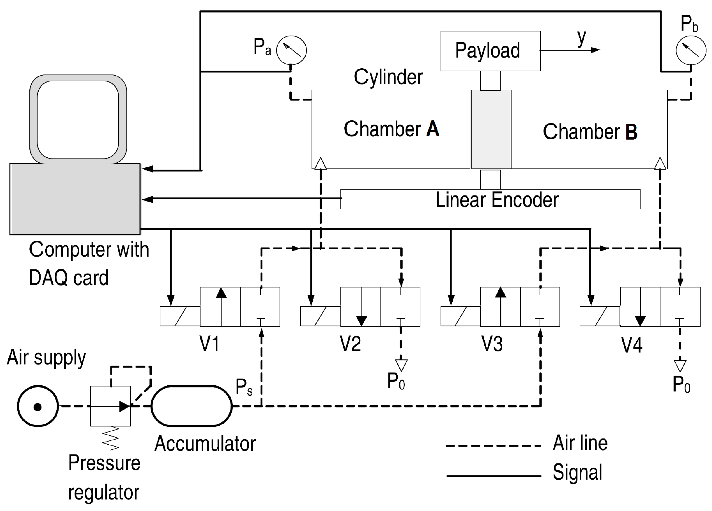
A schematic diagram of the pneumatic and electrical components of the position-controlled pneumatic actuator is presented in Figure 1. The double-acting cylinder can be rodded or rodless (as shown). The four two-way on/off solenoid poppet valves (labelled V1 to V4) allow the charging and discharging of the cylinder chambers, A and B, to be controlled independently. The piston position is measured by a linear incremental encoder. Two pressure sensors are used to measure the chamber pressures. The sensor and control signals are interfaced with a PC through a data acquisition card. With four on/off valves, the maximum number of operating modes is 16. In this work, we limit the modes to the set:

$$(\mathsf{\psi },v_1,v_2,v_3,v_4)\in \left\{\begin{array}{l}(1,\mathrm{on},\mathrm{off},\mathrm{off},\mathrm{on}),(2,\mathrm{off},\mathrm{on},\mathrm{on},\mathrm{off}),\\ (3,\mathrm{off},\mathrm{off},\mathrm{off},\mathrm{off})\end{array}\right\},$$

(1)

where $\mathsf{\psi }$ is the mode; $v_1$ to $v_4$ are the binary states of valves V1 to V4, respectively. These modes are identical to those used in [6] and [10]. Further details on the hardware used for experimental verification are presented in Section 5.1.

2.2. System Model

The chamber filling and discharging process are modeled as adiabatic. Based on the ideal gas, mass continuity, and energy conservation laws, the pressure dynamics for chambers A and B of the cylinder are

$$\mathsf{\gamma }RT{\dot{m}}_a=\mathsf{\gamma }{P}_a{\dot{V}}_a+V_a{\dot{P}}_a\mathrm{and}$$

(2)

$$\mathsf{\gamma }RT{\dot{m}}_b=\mathsf{\gamma }{P}_b{\dot{V}}_b+V_b{\dot{P}}_b,$$

(3)

where $\mathsf{\gamma }$ is the ratio of specific heats for air; $R$ is the universal gas constant; $T$ is the air temperature; ${\dot{m}}_a$ and ${\dot{m}}_b$ are the mass flow rates into chambers A and B; $P_a$ and $P_b$ are the chamber pressures; and $V_a$ and $V_b$ are the chamber volumes. The chamber volumes can be expressed by

$$V_a=A_{a}y\mathrm{and}$$

(4)

$$V_b=A_b\left(L-y\right),$$

(5)

where $y$ is the piston displacement, $A_a$ and $A_b$ are the cross-sectional areas of chambers A and B; and $L$ is the stroke length. Differentiating both sides of (4) and (5) gives

$${\dot{V}}_a=A_a\dot{y}\mathrm{and}$$

(6)

$${\dot{V}}_b=-A_b\dot{y}$$

(7)

After substituting (6) and (7), (2) and (3) can be rewritten as

$$\mathsf{\gamma }RT{\dot{m}}_a=\mathsf{\gamma }{A}_a\dot{y}{P}_a+A_{a}y{\dot{P}}_a\mathrm{and}$$

(8)

$$\mathsf{\gamma }RT{\dot{m}}_b=-\mathsf{\gamma }{A}_b\dot{y}{P}_b+A_b\left(L-y\right){\dot{P}}_b$$

(9)

The mass flow rates ${\dot{m}}_a$ and ${\dot{m}}_b$ into chambers A and B are

$${\dot{m}}_a={\dot{m}}_1-{\dot{m}}_2\mathrm{and}$$

(10)

$${\dot{m}}_b={\dot{m}}_3-{\dot{m}}_4,$$

(11)

where ${\dot{m}}_1$, ${\dot{m}}_2$, ${\dot{m}}_3$, and ${\dot{m}}_4$ are the mass flow rates through the four valves. To improve the modeling accuracy, suitable functions were chosen by studying experimental data and empirical curve fitting was adopted to model the flow behavior of the on/off valves. The mass flow rates through each valve are then given by

$${\dot{m}}_1\left(u,P_a\right)=\{\begin{array}{ll}{\mathsf{\lambda }}_{fill}\left(P_a\left(t_k\right)\right),& \mathrm{if}u\left(t_k-{\mathsf{\tau }}_{d,open}\right)=1\\ 0,& \mathrm{if}u\left(t_k-{\mathsf{\tau }}_{d,close}\right)\in \{2,3\}\end{array}$$

(12)

$${\dot{m}}_2\left(u,P_a\right)=\{\begin{array}{ll}{\mathsf{\lambda }}_{dis}\left(P_a\left(t_k\right)\right),& \mathrm{if}u\left(t_k-{\mathsf{\tau }}_{d,open}\right)=2\\ 0,& \mathrm{if}u\left(t_k-{\mathsf{\tau }}_{d,close}\right)=\{1,3\}\end{array}$$

(13)

$${\dot{m}}_3\left(u,P_a\right)=\{\begin{array}{ll}{\mathsf{\lambda }}_{fill}\left(P_b\left(t_k\right)\right),& \mathrm{if}u\left(t_k-{\mathsf{\tau }}_{d,open}\right)=2\\ 0,& \mathrm{if}u\left(t_k-{\mathsf{\tau }}_{d,close}\right)=\{1,3\}\end{array}$$

(14)

$${\dot{m}}_4\left(u,P_b\right)=\{\begin{array}{ll}{\mathsf{\lambda }}_{dis}\left(P_b\left(t_k\right)\right),& \mathrm{if}u\left(t_k-{\mathsf{\tau }}_{d,open}\right)=1\\ 0,& \mathrm{if}u\left(t_k-{\mathsf{\tau }}_{d,close}\right)=\{2,3\}\end{array}$$

(15)

$${\mathsf{\lambda }}_{fill}\left(P\right)=\{\begin{array}{ll}{c}_{choked}{P}_s,& \mathrm{if}{P}_s>\frac{P}{0.53}\\ c_{fill}\sqrt{P_s-P},& \mathrm{if}{P}_s\le \frac{P}{0.53}\end{array}\mathrm{and}$$

(16)

$${\mathsf{\lambda }}_{dis}\left(P\right)=\{\begin{array}{ll}{c}_{choked}P,& \mathrm{if}P>\frac{P_0}{0.53}\\ c_{dis}\left(P-P_0\right),& \mathrm{if}P\le \frac{P_0}{0.53}\end{array},$$

(17)

where $t_k$ is the time of the current sampling instant, $u$ is the commanded operating mode, ${\mathsf{\tau }}_{d,open}$ is the valve energizing delay time, ${\mathsf{\tau }}_{d,close}$ is the valve de-energizing delay time, $P_s$ is the supply pressure, $P_0$ is the atmospheric pressure, $c_{choked}$ is the choked mass flow rate coefficient, $c_{fill}$ is the chamber filling coefficient, and $c_{dis}$ is the chamber discharging coefficient.

The dynamics of the piston and payload are obtained using Newton’s second law as follows

$$M\ddot{y}=F_{\mathrm{p}}-F_{\mathrm{f}}+F_{\mathrm{ext}},$$

(18)

where $M$ is the total mass (i.e., sum of piston and payload masses), $F_{\mathrm{p}}=P_a{A}_a-P_b{A}_b$ is the pneumatic force, $F_{\mathrm{f}}$ is the friction force, and $F_{\mathrm{ext}}$ is the external force. It was empirically determined that the friction force was direction-dependent and included Stribeck, Coulomb, and viscous components. The friction force is modeled using

$$F_{\mathrm{f}}\left(\dot{y}\right)=\{\begin{array}{l}\begin{array}{ll}\left[F_{\mathrm{c},\mathrm{p}}+\left(F_{\mathrm{s},\mathrm{p}}-F_{\mathrm{c},\mathrm{p}}\right)e^{-{\left(\dot{y}/v_{\mathrm{s},\mathrm{p}}\right)}^2}\right]+C_{\mathrm{v},\mathrm{p}}\dot{y}& \dot{y}>0\\ -\left[F_{\mathrm{c},\mathrm{n}}+\left(F_{\mathrm{s},\mathrm{n}}-F_{\mathrm{c},\mathrm{n}}\right)e^{-{\left(\dot{y}/{\mathrm{v}}_{\mathrm{s},\mathrm{n}}\right)}^2}\right]+C_{\mathrm{v},\mathrm{n}}\dot{y}& \dot{y}<0\end{array}\\ F_{\mathrm{p}}+F_{\mathrm{ext}}\dot{y}=0\mathrm{and}0<F_{\mathrm{p}}+F_{\mathrm{ext}}<F_{\mathrm{s},\mathrm{p}}\\ F_{\mathrm{p}}+F_{\mathrm{ext}}\dot{y}=0\mathrm{and}-F_{\mathrm{s},\mathrm{n}}<F_{\mathrm{p}}+F_{\mathrm{ext}}<0\\ F_{\mathrm{s},\mathrm{p}}\dot{y}=0\mathrm{and}{F}_{\mathrm{p}}+F_{\mathrm{ext}}\ge F_{\mathrm{s},\mathrm{p}}\\ -F_{\mathrm{s},\mathrm{n}}\dot{y}=0\mathrm{and}{F}_{\mathrm{p}}+F_{\mathrm{ext}}\le -F_{\mathrm{s},\mathrm{n}}\end{array}$$

(19)

where $F_{\mathrm{c},\mathrm{p}}$ and $F_{\mathrm{c},\mathrm{n}}$ are the Coulomb friction forces for the positive and negative directions; $F_{\mathrm{s},\mathrm{p}}$ and $F_{\mathrm{s},\mathrm{n}}$ are the static friction forces for two directions; $v_{\mathrm{s},\mathrm{p}}$ and $v_{\mathrm{s},\mathrm{n}}$ are the Stribeck velocities for the two directions; and $C_{\mathrm{v},\mathrm{p}}$ and $C_{\mathrm{v},\mathrm{n}}$ are the viscous friction coefficients for the two directions. This friction model is similar to those studied in [14,15,16]. It has the advantage of capturing more of the complex behavior of the actuator’s friction than the ones used in [1,2,3,4,5,6,7,8,9,10,11,12].

2.3. Model Fitting and Validation

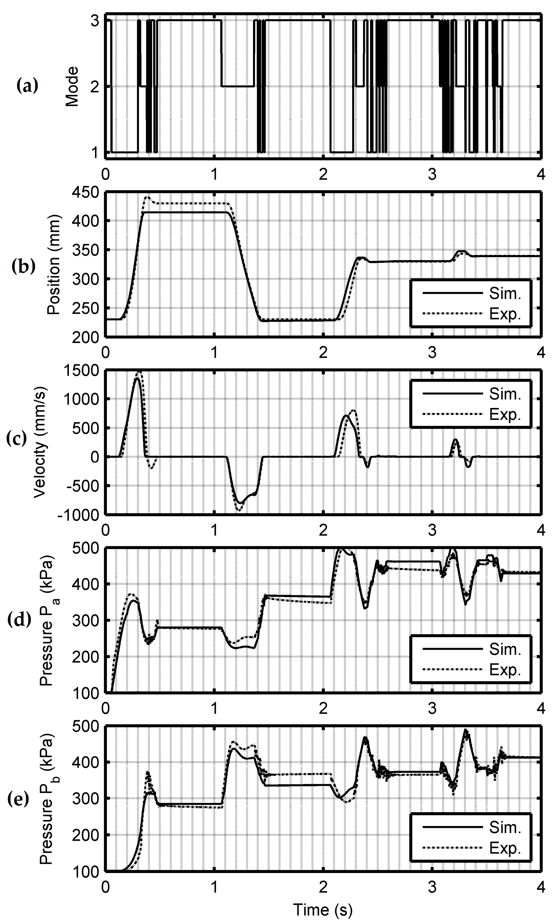
We used existing testing and curve fitting methods [16] to identify the valve and friction model parameters. The empirically identified model parameters for the test bed described in Section 5.1 are listed in

Table 1. System parameters.

Parameter	Value	Description
$T_s$	0.001 s	Sampling period
$A_a$	4.91 × 10−4 m2	Chamber A cross-sectional area
$A_b$	4.91 × 10−4 m2	Chamber B cross-sectional area
$T$	293 K	Air temperature
$L$	0.6 m	Cylinder stroke
$P_s$	6.0 × 105 Pa	Supply pressure (absolute)
$P_0$	1.0 × 105 Pa	Atmospheric pressure (absolute)
$M$	2.14 kg	Nominal total mass
${\tau }_{d,open}$	0.004 s	Valve energizing delay time
${\tau }_{d,close}$	0.001 s	Valve de-energizing delay time
$c_{fill}$	1.7 × 10−6 (m·kg) 0.5	Chamber filling coefficient
$c_{dis}$	6.1 × 10−9 m·s	Chamber discharging coefficient
$c_{choked}$	2.65 × 10−8 m·s	Choked mass flow rate coefficient
$F_{\mathrm{s},\mathrm{p}}$	54 N	Static friction force in the positive direction
$F_{\mathrm{s},\mathrm{n}}$	48 N	Static friction force in the negative direction
$F_{\mathrm{c},\mathrm{p}}$	81 N	Coulomb friction force in the positive direction
$F_{\mathrm{c},\mathrm{n}}$	78 N	Coulomb friction force in the negative direction
$C_{\mathrm{v},\mathrm{p}}$	7.9 N·s·m−1	Viscous friction coefficient in the positive direction
$C_{\mathrm{v},\mathrm{n}}$	23 N·s·m−1	Viscous friction coefficient in the negative direction
$v_{\mathrm{s},\mathrm{p}}$	0.37 m·s−1	Stribeck velocity in the positive direction
$v_{\mathrm{s},\mathrm{n}}$	0.36 m·s−1	Stribeck velocity in the negative direction

. Note that the large static and Coulomb friction forces are caused by the tight piston seals that are required to prevent leakage. A computer simulation was created using these parameters with the model equations from the previous section. The simulation and experimental results for the same sequence of commanded operating modes are compared in Figure 2. Note that the simulation was open-loop (i.e., it does not use any sensor data to predict the position, velocity, or pressures). The graphs show that the simulated model predicts the experimental results closely over a wide range of operating conditions.

3. Control Algorithms

3.1. SMC3

SMC3 was proposed in [6] and will be briefly summarized here. Its sliding surface is defined as

$$s=\frac{\ddot{e}}{{\mathsf{\omega }}^2}+\frac{2\mathsf{\xi }\dot{e}}{\mathsf{\omega }}+e$$

(20)

where $e=y_{\mathrm{d}}-y$ is the position error, $y$ is the actual position, $y_{\mathrm{d}}$ is the desired position, $\mathsf{\omega }$ is the desired natural frequency, and $\mathsf{\xi }$ is the desired damping ratio. The commanded mode is then

$$u=\{\begin{array}{l}1s>\mathsf{\epsilon }\\ 2s<-\mathsf{\epsilon }\\ 3-\epsilon \le s\le \mathsf{\epsilon }\end{array}$$

(21)

where $\mathsf{\epsilon }$ is a small positive dead band. The parameter $\mathsf{\epsilon }$ can be used to reduce the valve switching frequency at the cost of larger position errors.

3.2. DVMPC1

DVMPC was first proposed in [11]. In this section, DVMPC1, which is a modified version for the 3-mode case, is presented. For brevity in writing the prediction equations, we define:

$$t_j=t_k+j{T}_s$$

(22)

where $t_k$ is the time of the current sample, $T_s$ is the sampling period, and $t_j$ is the time $j$ samples into the future. The cost-function to be minimized is defined as:

$$J={\displaystyle \sum _{j=1}^{N_{\mathrm{p}}}\widehat{e}{\left(t_j\right)}^2}$$

(23)

where $\widehat{e}\left(t_j\right)=y_{\mathrm{d}}\left(t_j\right)-\widehat{y}\left(t_j\right)$ is the predicted tracking error, $\widehat{y}$ is the predicted position, $y_{\mathrm{d}}$ is the desired position, and $N_{\mathrm{p}}$ is the prediction horizon. The predicted optimal sequence of modes is then given by:

$$U_{\mathrm{opt}}=\arg \underset{U}{\min }J$$

(24)

subject to:

$$U=\left[\widehat{u}\left(t_k\right),\widehat{u}\left(t_k+T_s\right),...,\widehat{u}\left(t_k+\left(N_{\mathrm{p}}-1\right)T_{\mathrm{s}}\right)\right]$$

(25)

$$\widehat{u}\left(t_j\right)=\widehat{u}\left(t_k\right)\mathrm{for}j=\left\{1,2,...,N_{\mathrm{p}}\right\}$$

(26)

$$\widehat{u}\in \{1,2,3\}\mathrm{and}$$

(27)

$$\begin{array}{l}{\left[\widehat{y}\left(t_j\right),\widehat{\dot{y}}\left(t_j\right),{\widehat{P}}_a\left(t_j\right),{\widehat{P}}_b\left(t_j\right)\right]}^T=\\ f\left(\begin{array}{l}\widehat{u}\left(t_j-T_{\mathrm{s}}\right),\widehat{y}\left(t_j-T_{\mathrm{s}}\right),\widehat{\dot{y}}\left(t_j-T_{\mathrm{s}}\right),\\ {\widehat{P}}_a\left(t_j-T_{\mathrm{s}}\right),{\widehat{P}}_b\left(t_j-T_{\mathrm{s}}\right)\end{array}\right)\mathrm{for}j=\left\{1,2,...,N_{\mathrm{p}}\right\}\end{array}$$

(28)

The commanded operating mode,$u\left(t_k\right)$, is set equal to the first element of $U_{\mathrm{opt}}$. The search is limited by (26) to three possible solutions allowing the optimization problem to be easily solved by exhaustive search in real-time. The closed-loop performance may be tuned by changing the prediction horizon, $N_{\mathrm{p}}$. A zero-order hold with a period of $\max \left({\mathsf{\tau }}_{\mathrm{d},\mathrm{open}},{\mathsf{\tau }}_{\mathrm{d},\mathrm{close}}\right)$ is used to obtain reliable valve activation. The predictions in (28) are computed using the system model, Euler integration, backward differencing, and the sensed position and pressures. The details are given in Algorithm 1.

Algorithm 1: Prediction algorithm for DVMPC1
1	Set $p=0$, ${\widehat{P}}_a\left(t_p\right)=P_a\left(t_k\right)$, ${\widehat{P}}_b\left(t_p\right)=P_b\left(t_k\right)$, $\widehat{y}\left(t_p\right)=y\left(t_k\right)$ and $\widehat{\dot{y}}\left(t_p\right)=\left(y\left(t_k\right)-y\left(t_k-T_{\mathrm{s}}\right)\right)/T_{\mathrm{s}}$.
2	Compute $t_p=t_k+p{T}_{\mathrm{s}}$
3	If $t_p>t_k$, then use: ${\widehat{P}}_a\left(t_p\right)=P_a\left(t_p-T_{\mathrm{s}}\right)+T_{\mathrm{s}}{\widehat{\dot{P}}}_a\left(t_p-T_{\mathrm{s}}\right)$, ${\widehat{P}}_b\left(t_p\right)=P_b\left(t_p-T_{\mathrm{s}}\right)+T_{\mathrm{s}}{\widehat{\dot{P}}}_b\left(t_p-T_{\mathrm{s}}\right)$, $\widehat{y}\left(t_p\right)=\widehat{y}\left(t_p-T_{\mathrm{s}}\right)+T_{\mathrm{s}}\widehat{\dot{y}}\left(t_p-T_{\mathrm{s}}\right)$ and $\widehat{\dot{y}}\left(t_p\right)=\widehat{\dot{y}}\left(t_p-T_{\mathrm{s}}\right)+T_{\mathrm{s}}\widehat{\ddot{y}}\left(t_p-T_{\mathrm{s}}\right)$
4	Compute the predicted mass flow rates using: ${\widehat{\dot{m}}}_a\left(t_p\right)={\widehat{\dot{m}}}_1\left(\widehat{u}\left(t_p\right),{\widehat{P}}_a\left(t_p\right)\right)-{\widehat{\dot{m}}}_2\left(\widehat{u}\left(t_p\right),{\widehat{P}}_a\left(t_p\right)\right)$ and ${\widehat{\dot{m}}}_b\left(t_p\right)={\widehat{\dot{m}}}_3\left(\widehat{u}\left(t_p\right),{\widehat{P}}_b\left(t_p\right)\right)-{\widehat{\dot{m}}}_4\left(\widehat{u}\left(t_p\right),{\widehat{P}}_b\left(t_p\right)\right)$
5	Compute the predicted pressure derivatives using: ${\widehat{\dot{P}}}_a\left(t_p\right)=\left(\mathsf{\gamma }RT{\widehat{\dot{m}}}_a\left(t_p\right)-\mathsf{\gamma }{A}_a\widehat{\dot{y}}\left(t_p\right){\widehat{P}}_a\left(t_p\right)\right)/A_a\widehat{y}\left(t_p\right)$ and ${\widehat{\dot{P}}}_b\left(t_p\right)=\left(\mathsf{\gamma }RT{\widehat{\dot{m}}}_b\left(t_p\right)+\mathsf{\gamma }{A}_b\widehat{\dot{y}}\left(t_p\right){\widehat{P}}_b\left(t_p\right)\right)/A_b\left(L-\widehat{y}\left(t_p\right)\right)$
6	Compute the predicted pneumatic force using: ${\widehat{F}}_{\mathrm{p}}\left(t_p\right)={\widehat{P}}_a\left(t_p\right)A_a-{\widehat{P}}_b\left(t_p\right)A_b$
7	Substitute $\widehat{\dot{y}}\left(t_p\right)$, ${\widehat{P}}_a\left(t_p\right)$ and ${\widehat{P}}_b\left(t_p\right)$ into (19) to obtain the predicted friction force, ${\widehat{F}}_{\mathrm{f}}\left(t_p\right)$
8	Compute the predicted acceleration, $\widehat{\ddot{y}}\left(t_p\right)$, using (18), $M_{nom}$, ${\widehat{F}}_{\mathrm{p}}\left(t_p\right)$, and ${\widehat{F}}_{\mathrm{f}}\left(t_p\right)$
9	Set $p=p+1$
10	If $p<N_{\mathrm{p}}$, then go to Step 2
11	Stop

3.3. DVMPC2

In the NMPC literature, each change of the predicted control signal during the prediction horizon is termed a “move.” Move blocking [17] limits the number of allowed moves. While this strategy has the advantage of reducing the computational load, it also has the disadvantage of reducing the optimality of the solution. With DVMPC1, only one move (i.e., a change in $\widehat{u}\left(t_j\right)$ relative to $u\left(t_k-T_s\right)$) is allowed by (26) over the prediction horizon, so the resulting control may be far from the optimum obtained without move blocking. In order to improve the optimality, with DVMPC2 multiple moves are allowed in the optimization. The prediction horizon is now:

$$N_{\mathrm{p}}=N_{\mathrm{m}}{N}_{\mathrm{delta}}$$

(29)

where $N_{\mathrm{m}}$ is the number of moves, and $N_{\mathrm{delta}}$ is the prediction horizon used with each move. The cost-function for DVMPC2 is also changed to:

$$J={\displaystyle \sum _{j=1}^{N_{\mathrm{p}}}\widehat{e}{\left(t_j\right)}^2}+{\mathsf{\lambda }}_1{\displaystyle \sum _{j=1}^{N_{\mathrm{p}}}j{T}_{\mathrm{s}}\left|\widehat{e}\left(t_j\right)\right|}+{\mathsf{\lambda }}_2{N}_{psps}$$

(30)

where $N_{psps}$ is the number of predicted switches per second per valve (PSPS), ${\mathsf{\lambda }}_1$ is the weighting coefficient of the predicted integral of time-weighted absolute error (PITAE), ${\mathsf{\lambda }}_2$ is the weighting coefficient of the PSPS. The PSPS is obtained using:

$$N_{psps}=\frac{1}{4N_{\mathrm{p}}{T}_{\mathrm{s}}}{\displaystyle \sum _{j=1}^{N_{\mathrm{p}}}{S}_{p,j}}\mathrm{and}$$

(31)

$$S_{p,j}=\{\begin{array}{l}0\mathrm{if}\widehat{u}\left(t_j-T_s\right)=\widehat{u}\left(t_j\right)\\ 4\mathrm{if}\left(\widehat{u}\left(t_j-T_s\right)=1\wedge \widehat{u}\left(t_j\right)=2\right)\vee \left(\widehat{u}\left(t_j-T_s\right)=2\wedge \widehat{u}\left(t_j\right)=1\right)\\ 2\mathrm{otherwise}\end{array}$$

(32)

where $S_{p,j}$ is the number of predicted valve switches at time $t_j$.

Comparing (30) to (23), the addition of the weighted PITAE and PSPS terms improves DVMPC2’s ability to control the transient and steady-state position control performance and the switching frequency. The predicted optimal sequence of modes is then given by:

$$U_{\mathrm{opt}}=\arg \underset{U}{\min }J$$

(33)

subject to:

$$U=\left[\widehat{u}\left(t_k\right),\widehat{u}(t_k+N_{\mathrm{delta}}{T}_{\mathrm{s}}),...,\widehat{u}(t_k+N_m{N}_{\mathrm{delta}}{T}_{\mathrm{s}})\right]$$

(34)

$$\begin{array}{r}\widehat{u}\left(t_k+\left(j+m{N}_{delta}\right)T_s\right)=\widehat{u}\left(t_k\right)\mathrm{for}j=\left\{1,2,...,N_{\mathrm{delta}}\right\}\\ \mathrm{and}m=\left\{1,2,...,N_{\mathrm{m}}\right\}\end{array}$$

(35)

$$\widehat{u}\in \{1,2,3\}$$

(36)

$$\begin{array}{l}{\left[\widehat{y}\left(t_j\right),\widehat{\dot{y}}\left(t_j\right),{\widehat{P}}_a\left(t_j\right),{\widehat{P}}_b\left(t_j\right)\right]}^T=\\ f\left(\widehat{u}\left(t_j-T_{\mathrm{s}}\right),\widehat{y}\left(t_j-T_{\mathrm{s}}\right),\widehat{\dot{y}}\left(t_j-T_{\mathrm{s}}\right),{\widehat{P}}_a\left(t_j-T_{\mathrm{s}}\right),{\widehat{P}}_b\left(t_j-T_{\mathrm{s}}\right)\right)\mathrm{for}j=\left\{1,2,...,N_{\mathrm{p}}\right\}\end{array}$$

(37)

$$V(t_k+N_{\mathrm{p}}\cdot T_{\mathrm{s}})<V(t_k)\vee V(t_k+N_{\mathrm{p}}\cdot T_{\mathrm{s}})<V_{\mathrm{threshold}}$$

(38)

where $V={\left(y_{\mathrm{d}}-y\right)}^2+d{\left({\dot{y}}_{\mathrm{d}}-\dot{y}\right)}^2$ is a Lyapunov-like function, and d is a positive weighting coefficient. The constraint (38) is used to guarantee the bounded-input, bounded-output stability of the nominal system. Only the errors of position and velocity are included in the Lyapunov-like function V. The chamber pressures are already bounded by $P_s$ and $P_0$, and leaving them out of V gives the optimization more freedom when minimizing J. The constraint (38) includes two inequalities. The first inequality, $V(t_k+N_{\mathrm{p}}\cdot T_{\mathrm{s}})<V(t_k)$ will be satisfied if V decreases over the prediction horizon, which implies that the position and velocity errors have also decreased. Unfortunately, even in the nominal case, this inequality will not always hold due to the control signal being discrete-valued and the finite prediction horizon. As mentioned in [10], steady-state errors or limit cycles can occur with this type of system. For these reasons, it was necessary to include the second inequality, $V(t_k+N_{\mathrm{p}}\cdot T_{\mathrm{s}})<V_{\mathrm{threshold}}$. This inequality guarantees that the position and velocity errors are bounded for the nominal system. Specifically, the error vector ${\left[e\hspace{1em}\dot{e}\right]}^T$ is forced inside an ellipse that is centered at the origin. The dimensions of the ellipse are determined by the choices of $V_{\mathrm{threshold}}$ and d. Note that for small values of $V_{\mathrm{threshold}}$ the optimization problem can become infeasible. So, choosing $V_{\mathrm{threshold}}$ involves a trade-off between feasibility and stability with DVMPC2. Note that the cost function (30) and stability constraint (38) are different than those used in the prior papers [9,10,11,12].

The use of move blocking in (33) to (38) reduces the search space from $3^{N_{\mathrm{p}}}$ to $3^{N_{\mathrm{m}}}$ nodes. So the computational load grows exponentially with $N_{\mathrm{m}}$. With NMPC, a larger $N_{\mathrm{p}}$ tends to improve the closed-loop performance. Since $N_{\mathrm{p}}=N_{\mathrm{m}}{N}_{\mathrm{delta}}$, $N_{\mathrm{delta}}$, and $N_{\mathrm{p}}$ can be increased without increasing the computational load of this ILP. However, larger $N_{\mathrm{delta}}$ values will block more moves and reduce the optimality of the solution (as previously mentioned), so there is a trade-off when choosing $N_{\mathrm{delta}}$. To allow larger values of $N_{\mathrm{m}}$ and $N_{\mathrm{p}}$ to be used with the chosen $N_{\mathrm{delta}}$, the search algorithm used with DVMPC2 is the efficient SDFS algorithm from [9] instead of the exhaustive search employed with DVMPC1.

The commanded operating mode,$u\left(t_k\right)$, is set equal to the first element of $U_{\mathrm{opt}}$. The zero-order hold and prediction algorithm for computing (37) are the same as with DVMPC1. The closed-loop performance may be tuned using the parameters $N_{\mathrm{m}}$, $N_{\mathrm{delta}}$, ${\mathsf{\lambda }}_1$ and ${\mathsf{\lambda }}_2$.

4. Controller Parameter Optimization

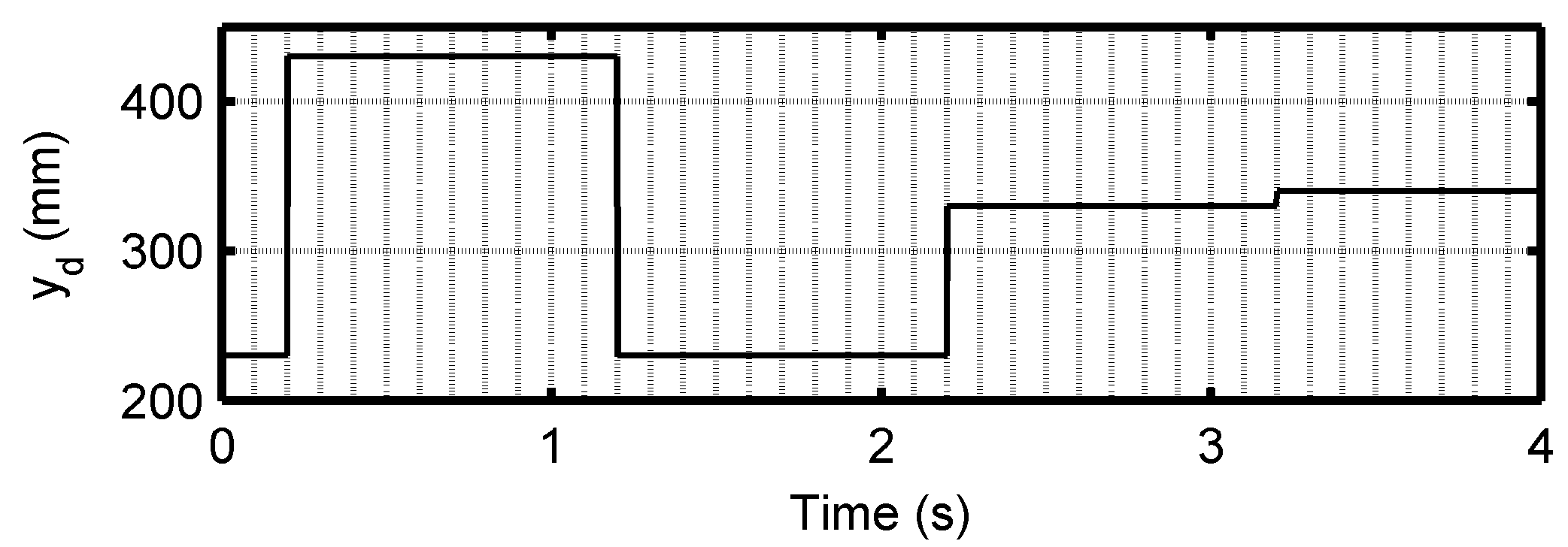
To make the comparison of the SMC3, DVMPC1, and DVMPC2 controllers fair their parameters will be tuned using optimization. A multi-step desired position trajectory is used so their performance will be evaluated under dynamic and steady-state conditions. Figure 3 shows the desired trajectory. The step heights are 200 mm, –200 mm, 100 mm and 10 mm. The total duration is 4 s.

Many metrics may be used to evaluate the performance of control systems. We have chosen the metrics integral of time-weighted absolute error (ITAE) and the number of switches per second per valve (SPS) to make quantitative comparisons. The ITAE is calculated in the normal manner, while the SPS is obtained using

$$\mathrm{SPS}=\frac{1}{4n{T}_{\mathrm{s}}}{\displaystyle \sum _{k=1}^n{S}_k}\mathrm{and}$$

(39)

$$S_k=\{\begin{array}{l}0\mathrm{if}u\left((k-1)T_s\right)=u\left(k{T}_s\right)\\ 4\mathrm{if}\left(u\left((k-1)T_s\right)=1\wedge u\left(k{T}_s\right)=2\right)\vee \\ \left(u\left((k-1)T_s\right)=2\wedge u\left(k{T}_s\right)=1\right)\\ 2\mathrm{otherwise}\end{array}$$

(40)

where n is the number of data points.

The next issue was deciding how to formulate the optimization using these two metrics. One option was to define the cost function as the weighted average of the two metrics. This was rejected since the chosen weighting coefficients may favor one controller more than the others. We instead chose to minimize one of the metrics and use the others in the constraints. The optimal controller parameters are then given by:

$$X_{opt}=\arg \underset{X}{\min }\mathrm{ITAE}$$

(41)

subject to:

$$\mathrm{SPS}\le {\mathrm{SPS}}_{\max }$$

(42)

$$X_{LB}\le X\le X_{UB}$$

(43)

where X is the vector of parameters; $X_{opt}$ is the optimal vector of parameters; ${\mathrm{SPS}}_{\max }$ is the upper bound on the SPS; and $X_{LB}$ and $X_{UB}$ define the lower and upper bounds of the elements of X, respectively.

The ITAE is minimized in (41) since it provides a measurement of both the transient and steady-state performance. The bound ${\mathrm{SPS}}_{\max }=15{\mathrm{s}}^{-1}$ was chosen based on the SPS values obtained when the controllers were manually tuned.

The mesh adaptive direct search (MADS) optimization algorithm [18] was chosen to solve (41)–(44) since it is well suited to blackbox problems of this type. The software library NOMAD (an abbreviation of Nonlinear Optimization by MADS) [19] was used to perform the optimization. Although more optimal parameters would have been obtained if the optimization was performed based on experiments, the optimization was based on simulations of the closed-loop system. There are three good reasons for employing simulation-based optimization. First, the optimizer may choose parameters that cause the response to be unstable, resulting in damage to the equipment. Second, the optimization may require the cost to be computed thousands of times, so the required number of experiments could take an excessive amount of time. Third, the large number of experiments would shorten the life of the equipment. The system parameters used in the simulations are listed in Table 1.

Each optimization run terminated successfully when the minimum mesh size was reached. The optimization results for SMC3 and DVMPC1 are: $\mathsf{\omega }=86.9$ rad/s, $\mathsf{\xi }=1.77$, and $\mathsf{\epsilon }=0.52$ mm; and $N_{\mathrm{p}}=61$. The results for DVMPC2 are $N_{\mathrm{m}}=4$, $N_{\mathrm{delta}}=32$, ${\mathsf{\lambda }}_1=0.0269$, ${\mathsf{\lambda }}_2=2.50$, $V_{\mathrm{threshold}}=93.3{\mathrm{mm}}^2$, and $d=1.94\times {10}^{-5}{\mathrm{s}}^2$.

5. Experimental Verification

5.1. Testbed

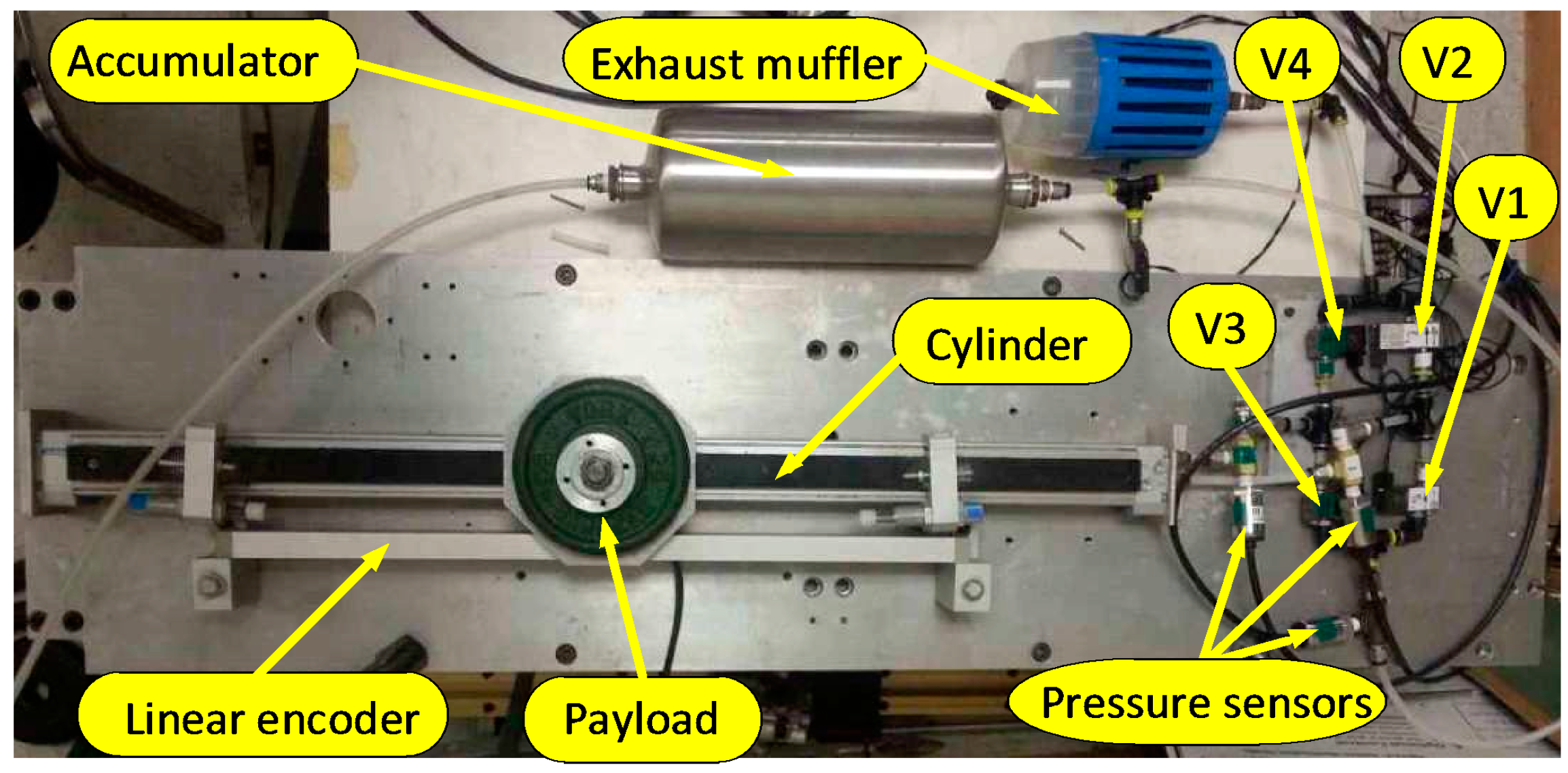
A photograph of the hardware used to test the three control algorithms is shown in Figure 4. The cylinder (made by Festo, model number DGPL-25-600) is rodless with a 600 mm stroke and 25 mm bore. The cylinder includes an exterior linear bearing for supporting the moving mass. The four on/off solenoid poppet valves are made by MAC with model number 34B-AAA-GDFB-1BA. The resolution of the linear incremental encoder is 0.01 mm. The three pressure sensors are made by SSI Technologies with model number P51-100. Low-pass filters with a 95 Hz cutoff frequency are used with the pressure sensors to reduce high-frequency noise and prevent aliasing. The data acquisition card is made by National Instruments with model number PCIe-6365. The sampling frequency is 1 kHz. The control algorithms are executed on a PC with a 3.4 GHz Intel i7-6700 processor and 8.0 GB RAM and are programmed in C language. The supply pressure was set to 0.6 MPa. The nominal total mass is 2.14 kg.

5.2. Experimental Results and Discussion

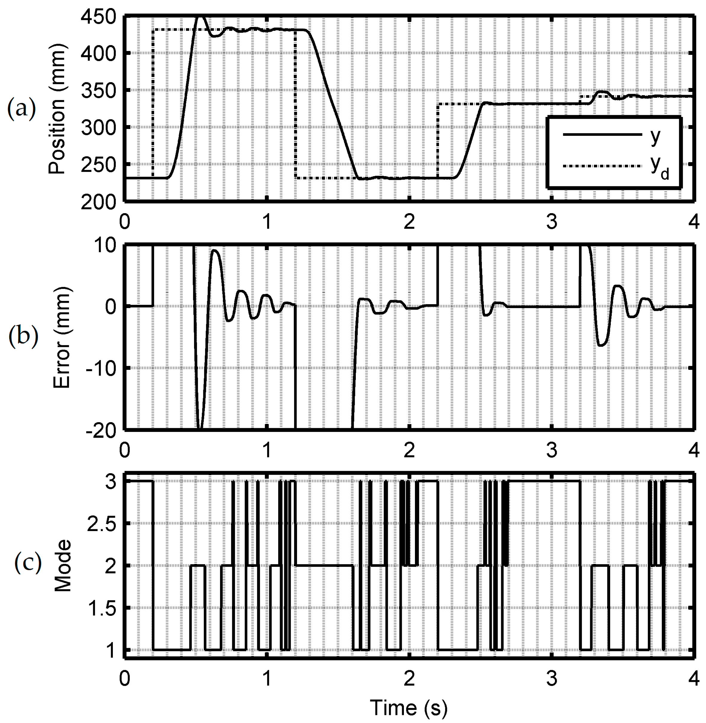
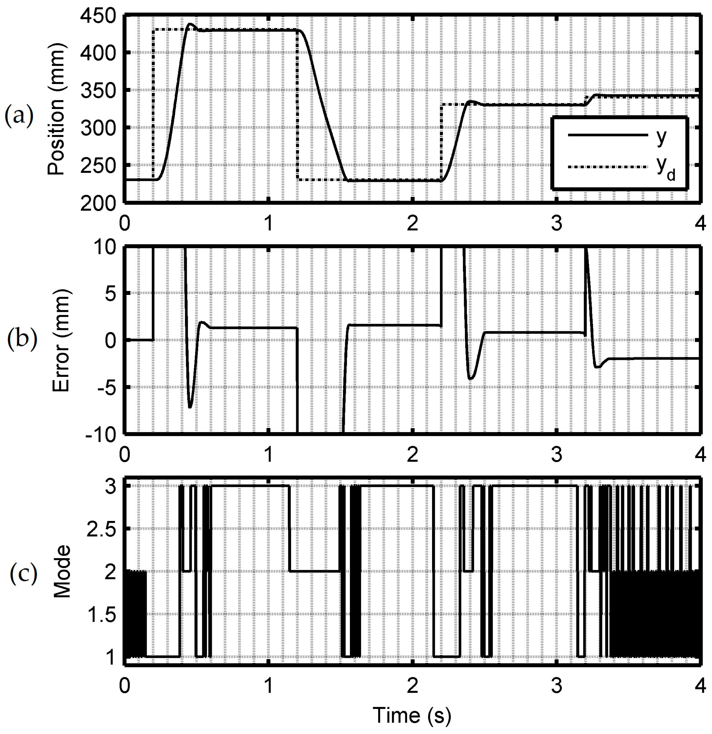
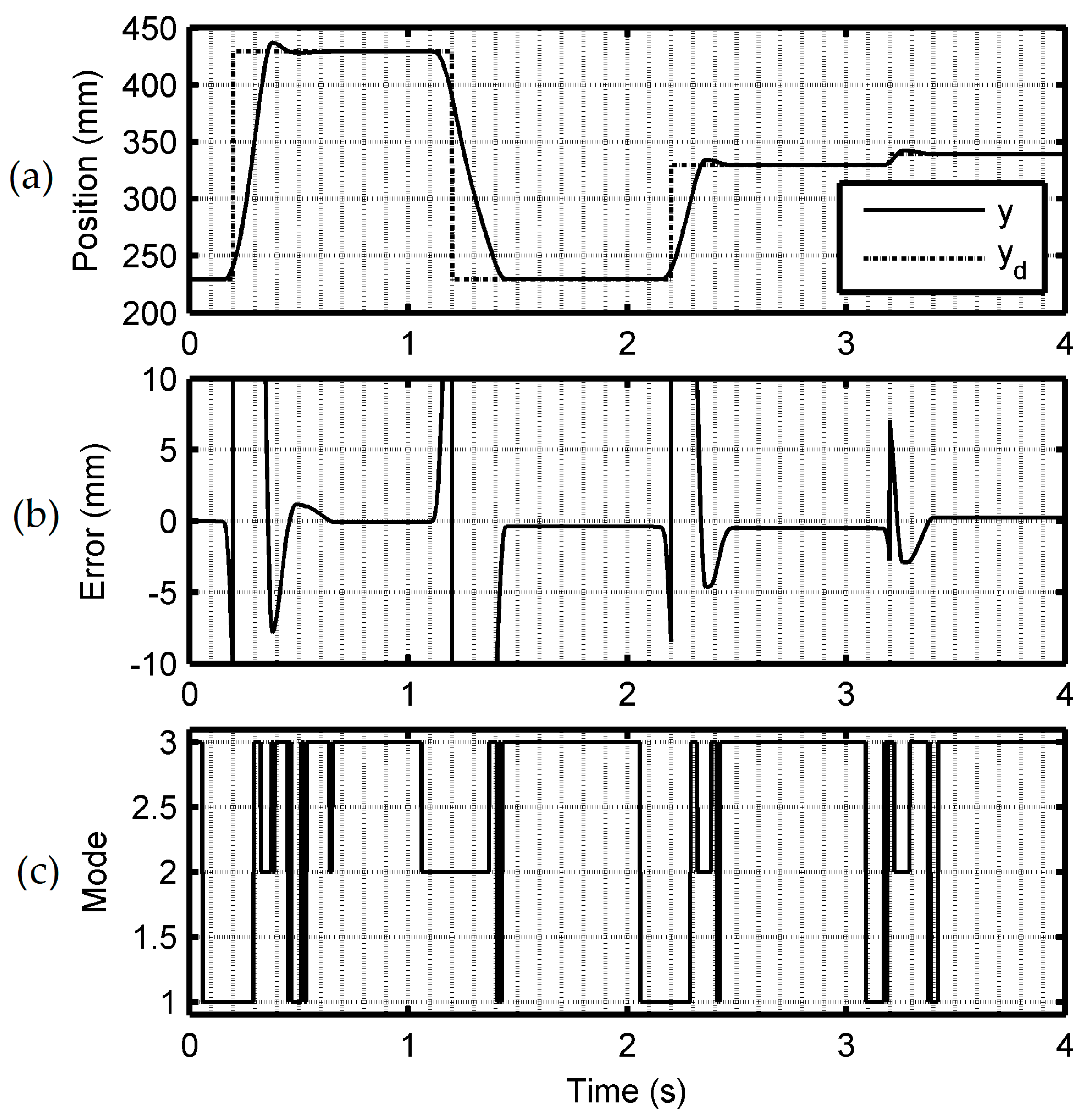
The experiments were performed using the controller parameters from Section 4 and the desired position trajectory shown in Figure 3. Typical experimental results for SMC3, DVMPC1, and DVMPC2 with the nominal total mass are plotted in Figure 5, Figure 6 and Figure 7, respectively. It is clear from these plots that DVMPC1 and DVMPC2 produced much fewer position oscillations than SMC3. With DVMPC1, this improved position control came at the cost of greater valve switching. However, DVMPC2 was able to both improve the smoothness of the position response and reduce the amount of valve switching. The performance metrics for these nominal results and for the tests with mass mismatch are given in

Table 2. Experimental results.

Controller Type	Total mass (kg)	SPS (s−1)	RMSE (mm)	ITAE (smm)	SSE (mm)	OS (mm)
SMC3	2.14	7.75	64.7	15.81	0.876	8.02
DVMPC1	2.14	22.08	51.3	7.98	1.145	4.16
DVMPC2	2.14	5.70	32.2	2.95	0.578	3.78
SMC3	3.36	7.80	63.3	16.99	1.637	12.56
DVMPC1	3.36	25.43	51.0	9.07	1.778	8.71
DVMPC2	3.36	7.25	32.3	3.81	1.172	8.11
SMC3	0.95	7.20	60.9	11.71	0.326	1.92
DVMPC1	0.95	36.23	48.5	6.78	0.968	0.67
DVMPC2	0.95	5.15	26.7	2.34	0.782	1.03

. The tabulated values are the averages from five experiments. For four of the five metrics, DVMPC2 was superior to DVMPC1 and outperformed SMC3 by a wide margin. Based on the averaged results for the nominal and mass mismatch cases, DVMPC2 reduced ITAE by 80%, RMSE by 52%, OS by 43% and SPS by 20% relative to SMC3. There was no clear winner in terms of SSE.

Regarding the controllers’ robustness, ITAE experienced the largest change of the four metrics. When the total mass was 3.36 kg (57% larger than nominal), the ITAE increases for SMC3, DVMPC1, and DVMPC2 were 7%, 14%, and 29%, respectively. These results make sense since the model-based DVMPC algorithms should be more sensitive than SMC3. A decrease in the mass should allow it to reach the desired position faster, causing the ITAE to decrease. When the mass was reduced to 0.95 kg (56% smaller than nominal), the decreases in the ITAE for SMC3, DVMPC1, and DVMPC2 were 26%, 15%, and 21%, respectively. The ITAE with the DVMPC algorithms benefited less from the reduction in mass since they were negatively affected by the model mismatch.

6. Conclusions

We have presented the development of an improved NMPC algorithm, termed DVMPC2, for the position control of double-acting pneumatic cylinders using on/off valves. Even though they make precise position control more challenging, we chose to use on/off valves since the resulting cost-savings (compared to the proportional valves used with the majority of pneumatic servo systems) increases the number of potential applications of pneumatic servo systems in robotics and automation. Similarly, we designed DVMPC2 to directly switch the valves to reduce the switching frequency, compared with the commonly used PWM approach, in order to reduce the costs of repairing or replacing valves worn out by switching. DVMPC2 has several other advantages. Its prediction strategy is superior to the strategy used in [11] and [12]. Its combination of move blocking and SDFS allows it to be computed in real-time on common hardware. It is also not necessary to simplify the dynamic model as was done in [10]. Finally, its cost function has four adjustable parameters making it much more flexible than the cost functions employed in [9,10,11,12].

After optimally tuning the parameters to make the comparison fair, we compared the performance of DVMPC2 with DVMPC1 and SMC3 for a multi-step desired position trajectory. The comparison was based on five performance metrics. Robustness was evaluated by introducing a mismatch between the nominal and actual total masses. The experimental results demonstrated the superior performance of DVMPC2 in terms of the ITAE, RMSE, OS, and SPS metrics. This means that DVMPC2 provides better position tracking while simultaneously extending the lives of the valves. This research is ongoing. As mentioned in Section 1, a 7-mode SMC algorithm was proposed in [8] and shown to outperform the SMC3 algorithm in terms of OS and SPS. An obvious extension to DVMPC2 is to expand from three modes to the seven modes used in [7]. However, this will increase the maximum number of nodes to be searched from $3^{N_{\mathrm{m}}}$ to $7^{N_{\mathrm{m}}}$. Since reducing $N_{\mathrm{m}}$ will be detrimental to the closed-loop performance, and we want to continue using common hardware to implement the controller, we are working on more efficient strategies to solve the resulting INP in real-time.

References

- Van Varseveld, R.B.; Bone, G.M. Accurate position control of a pneumatic actuator using on/off solenoid valves. IEEE/ASME Trans. Mechatron. 1997, 2, 195–204. [Google Scholar] [CrossRef]
- Shen, X.; Zhang, J.; Barth, E.J.; Goldfarb, M. Nonlinear model-based control of pulse width modulated pneumatic servo systems. ASME J. Dyn. Syst. Meas. Control 2006, 128, 663–669. [Google Scholar] [CrossRef]
- Hodgson, S.; Tavakoli, M.; Pham, M.T.; Leleve, A. Nonlinear discontinuous dynamics averaging and PWM-based sliding mode control of solenoid-valve pneumatic actuators. IEEE/ASME Trans. Mechatron. 2015, 20, 876–888. [Google Scholar] [CrossRef]
- Mazare, M.; Taghizadeh, M.; Kazemi, M.G. Optimal hybrid scheme of dynamic neural network and PID controller based on harmony search algorithm to control a PWM-driven pneumatic actuator position. J. Vib. Control 2018, 24, 3538–3554. [Google Scholar] [CrossRef]
- Paul, A.K.; Mishra, J.K.; Radke, M.G. Reduced order sliding mode control for pneumatic actuator. IEEE Trans. Control Syst. Technol. 1994, 2, 271–276. [Google Scholar] [CrossRef]
- Barth, E.J.; Goldfarb, M. A control design method for switching systems with application to pneumatic servo systems. In Proceedings of the ASME International Mechanical Engineering Congress and Exposition, New Orleans, LA, USA, 17–22 November 2002; pp. 463–469. [Google Scholar]
- Nguyen, T.; Leavitt, J.; Jabbari, F.; Bobrow, J.E. Accurate sliding-mode control of pneumatic systems using low-cost solenoid valves. IEEE/ASME Trans. Mechatron. 2007, 12, 216–219. [Google Scholar] [CrossRef]
- Hodgson, S.; Le, M.Q.; Tavakoli, M.; Pham, M.T. Improved tracking and switching performance of an electro-pneumatic positioning system. Mechatronics 2012, 22, 1–12. [Google Scholar] [CrossRef] [Green Version]
- Wu, J.; Abdelwahed, S. Discrete-input receding horizon control applied to pneumatic hopping robot energy regulation. In Proceedings of the IEEE International Conference on Systems, Man and Cybernetics, Montréal, QC, Canada, 7–10 October 2007; pp. 1567–1572. [Google Scholar]
- Grancharova, A.; Johansen, T.A. Design and comparison of explicit model predictive controllers for an electropneumatic clutch actuator using On/Off valves. IEEE/ASME Trans. Mechatron. 2011, 16, 665–673. [Google Scholar] [CrossRef]
- Bone, G.M.; Chen, X. Position control of hybrid pneumatic-electric actuators. In Proceedings of the American Control Conference, Montréal, QC, Canada, 27–29 June 2012; pp. 1793–1799. [Google Scholar]
- Bone, G.M.; Xue, M.T.; Flett, J. Position control of hybrid pneumatic–electric actuators using discrete-valued model-predictive control. Mechatronics 2015, 25, 1–10. [Google Scholar] [CrossRef]
- Jünger, M.; Liebling, T.; Naddef, D.; Nemhauser, G.; Pulleyblank, W.; Reinelt, G. (Eds.) 50 Years of Integer Programming 1958–2008: From the Early Years to the State-of-the-Art; Springer: Berlin, Germany, 2010. [Google Scholar]
- Nouri, B.M.Y.; Al-Bender, F.; Swevers, J.; Vanherck, P.; Van Brussel, H. Modelling a pneumatic servo positioning system with friction. In Proceedings of the American Control Conference, Chicago, IL, USA, 28–30 June 2000; pp. 1067–1071. [Google Scholar]
- Andrighetto, P.L.; Valdiero, A.C.; Carlotto, L. Study of the friction behavior in industrial pneumatic actuators. In Proceedings of the ABCM Symposium Series in Mechatronics, Ouro Preto, Brazil, 6–11 November 2005; pp. 369–376. [Google Scholar]
- Rao, Z.; Bone, G.M. Nonlinear modeling and control of servo pneumatic actuators. IEEE Trans. Control Syst Technol. 2008, 16, 562–569. [Google Scholar]
- Cagienard, R.; Grieder, P.; Kerrigan, E.C.; Morari, M. Move blocking strategies in receding horizon control. J. Proc. Control 2007, 17, 563–570. [Google Scholar] [CrossRef] [Green Version]
- Audet, C.; Dennis, J.E. Mesh adaptive direct search algorithms for constrained optimization. SIAM J. Optim. 2006, 17, 188–217. [Google Scholar] [CrossRef]
- Le Digabel, S. Algorithm 909: NOMAD: Nonlinear optimization with the MADS algorithm. ACM Trans. Math. Softw. 2011, 37, 44–59. [Google Scholar] [CrossRef]
Figure 1.
System schematic.
Figure 2.
Comparison of simulation and experimental results plotted vs. time. (a) Commanded valve operating mode; (b) Positions; (c) Velocities; (d) Chamber A pressures; and (e) Chamber B pressures.
Figure 3.
Multi-step desired position trajectory.
Figure 4.
Test bed used for the experiments (PC and electronics are not shown).
Figure 5.
Experimental result for 3-mode sliding-mode control algorithm (SMC3) with the nominal total mass. (a) Desired position, , and sensed position, ; (b) Position error, ; and (c) Commanded valve operating mode, .
Figure 6.
Experimental result for discrete-valued model-predictive control 1 (DVMPC1) with the nominal total mass. (a) Desired position, , and sensed position, ; (b) Position error, ; and (c) Commanded valve operating mode, .
Figure 7.
Experimental result for discrete-valued model-predictive control 2 (DVMPC2) with the nominal total mass. (a) Desired position, , and sensed position, ; (b) Position error, ; and (c) Commanded valve operating mode, .