Mechatronic Control System for a Compliant and Precise Pneumatic Rotary Drive Unit

Abstract

Robots that enable safe human-robot collaboration can be realized by using compliant drive units. In previous works, different mechanical designs of compliant pneumatic rotary drive units with similar characteristics have been presented. In this paper, we present the overall control approach that we use to operate one of these compliant pneumatic rotary drive units. We explain the mechanical design and derive the differential equation that describes the dynamics of the system. In order to successfully operate a pneumatic drive unit with three or more working chambers, the torque specified by the controller has to be split up onto the working chambers. We transfer the well-known field-oriented control approach from electric motors to the investigated pneumatic drive unit to create such a torque mapping. Moreover, we develop optimized torque mappings that are tailored to work with this type of drive unit. Furthermore, we introduce and compare two control algorithms based on different implementations of state feedback to realize position control. Finally, we present the step responses that we achieve when we implement either one of the control algorithms in combination with the different torque mappings.

1. Introduction

1.1. Motivation

Pneumatic drive units feature intrinsic compliance due to the compressibility of pressurized air. Hence, this characteristic makes pneumatic drive units very interesting for all robotic applications in which compliance is mandatory. Thus, using pneumatic drive units is one possibility to realize robots capable of safe human-robot collaboration. In the pending patent, [1], several possible mechanical designs for drive units with similar characteristics are presented. In previous works, two drive units with very similar characteristics were designed in detail and laboratory test stands have been realized. Moreover, these drive units were successfully tested, characterized, and the capabilities for the potential use in robotics, especially in human-robot collaboration, were demonstrated.

Every pneumatic actuation element uses a working chamber. When we fill the working chamber with compressed air, it is deformed, and this deformation causes the pneumatic actuation element to exert a certain type of force onto the system. The main idea behind these new mechanical designs is to avoid the well-known stick-slip phenomenon that is usually generated through the contact of the seal and the cylinder wall. Most of the pneumatic actuation elements used today are classic pneumatic cylinders that use a piston and a seal to realize airtight pneumatic working chambers. To avoid the stick-slip phenomenon, we designed drive units that do not use seals to seal the working chamber against the ambient pressure. Instead, both drive units use working chambers with elastic walls and thus variable volume. Hence, both drive units avoid control problems originating from the above-mentioned stick-slip phenomenon.

In [2], we introduced a rotary drive using bellow actuators while we presented a rotary drive using pneumatic artificial muscles (PAMs) in [3]. We have reached the accuracy of the implemented 16-bit encoder, resolving ${0.0055}^{\circ }$ with both laboratory test stands. Consequently, both drive units are capable of high-precision positioning.

However, a suitable control system for these new types of pneumatic drive units has not yet been presented. To operate and characterize the aforementioned drive units, a control system for position control of pneumatic rotary drive units with three or more working chambers is necessary. In the present work, we, therefore, explain and evaluate the mechatronic control system that we have realized to perform position control with the drive unit presented in [3]. This particular pneumatic rotary drive unit uses three to five PAMs as working chambers.

1.2. Related Works

A general introduction to PAMs is given in [4]. A survey on different modeling approaches for PAMs is presented in [5]. The relations between applied pressure, current extension, and exerted force of a PAM are quite well understood and different models are described in [6,7,8,9]. Pneumatic drive units are in most cases designed with two identical but antagonistic working chambers. As a result, many control approaches are investigating antagonistic configurations of various types of working chambers. The design of a rotary drive with two antagonistic gaiters is presented in [10] and the control of this system is presented in [11]. Fiber-reinforced gaiters are used in an antagonistic setup to create a robotic joint, see [12]. The control of single PAMs is presented in [8,13,14] and the control of drive configuration comprising two antagonistic PAMs is presented in [15,16,17,18,19,20]. Besides the configurations with identical but antagonistic working chambers, configurations with different types of antagonistic elements are also described in research. For example, an antagonistic system comprising a PAM and a spring is described in [21]. In antagonistic drive configurations, there is always only one working chamber capable of causing a positive or negative torque output on the drive shaft at any position within the rotatory range of the drive unit. Hence, there is no need in the above-mentioned cases to split the desired torque level up and distribute it over multiple working chambers. For the drive unit that we operate in the present work, a torque distribution is mandatory to successfully operate and control the available drive unit. We call this transformation “torque mapping” within the presented control approach. The torque mapping problem, distributing a given torque over multiple actuators, has been solved for electric AC-motors within the theory of the so-called field-oriented-control (FOC) or vector control. Within the FOC, the Park–Clarke transform, also called direct-quadrature-zero transformation (DQZ transform), solves the torque mapping problem for AC-motors. The complete DQZ approach is well-known and for example described in [22,23,24].

1.3. Contribution of the Present Work

The fundamental idea behind the control approach presented in this work is to transfer the DQZ torque mapping from field-oriented-control of electric motors to work with the aforementioned pneumatic rotary drive unit. In two student works, basic controllers for position control have been created and tested. Both controllers are based on state-feedback-control and they are initially combined with the underlying and unmodified standard DQZ torque mapping, see [25,26]. We present these controllers and we introduce three modified torque mappings that we have developed to improve the performance of the position control. Finally, we present measurements of the step response for different combinations of torque mappings and controllers.

1.4. Overview of the Present Work

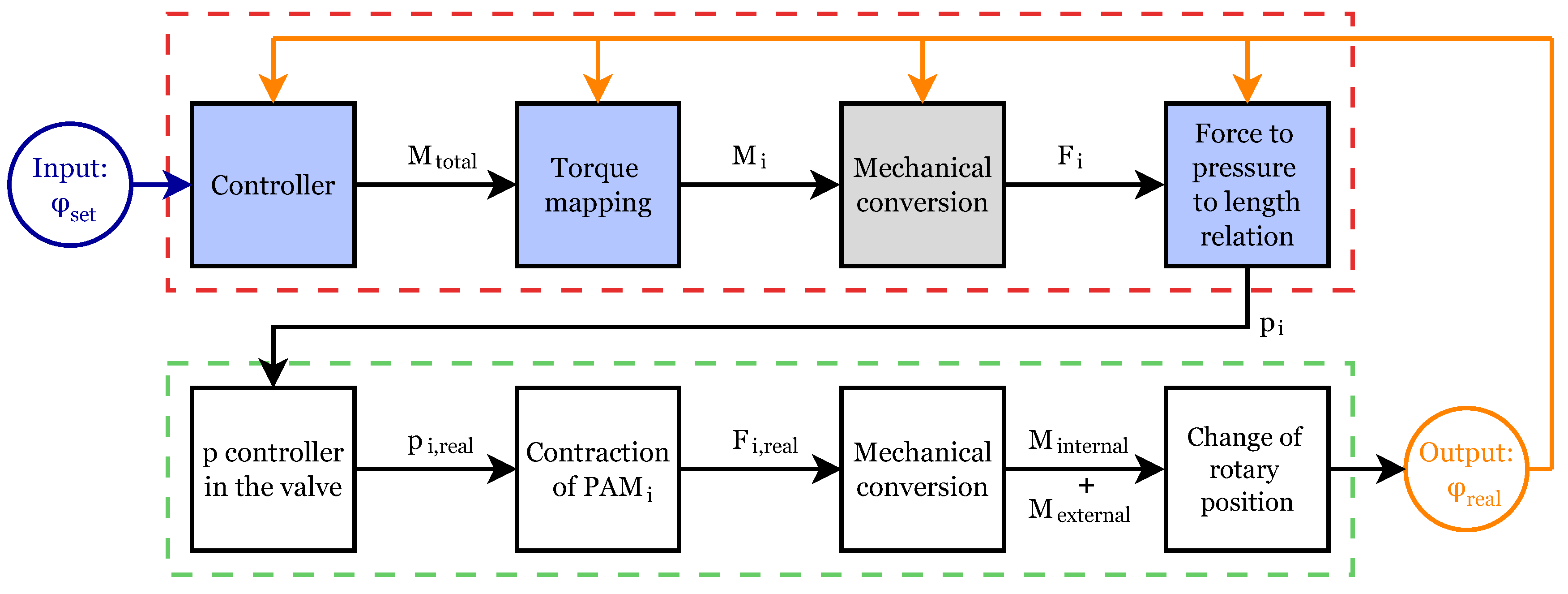
In this work, we propose a mechatronic control system for a pneumatic rotary drive unit that comprises three or more working chambers. We derive all theoretic equations and we describe all components that we developed to finally realize a position control. We go through the control scheme presented in Figure 1 and explain the blue colored boxes in detail. In Section 2, we briefly introduce the available laboratory test stands, including the pneumatic and electronic control components. Hereafter, we derive the differential equation, based on the principle of angular momentum. The modelling that represents our rotary drive unit is described in Section 3. In Section 4, we introduce four different torque mappings followed by Section 5, where we explain the two different controllers that we developed. Moreover, we present measurements of the step response of the drive unit in Section 6, and we discuss these results in Section 7. Finally, we sum up the present work and we give an outlook on possible future research in Section 8.

2. Mechanical Design and Laboratory Test Stand

2.1. Mechanical Design

The mechanical design of two different, compliant pneumatic rotary drive units has been presented in [2,3]. Both designs are capable of high-precision positioning, ${360}^{\circ }$ continuous rotation, and both designs enable adjustable stiffness. The first developed drive unit, presented in [2], comprises three bellow elements as working chambers. These bellows exert a pushing force. Unfortunately, the bellow elements used in this design show a low durability. Therefore, this drive unit cannot be used to realize and investigate control approaches. Thus, we do not further consider this drive unit in the present work.

Unlike these particular bellow elements, pneumatic artificial muscles (PAMs) are a standard industry product and thus very durable. Hence, the second drive unit, described in [3], comprises three to five PAMs in a modular design. The PAMs used in this design exert pulling forces onto the system.

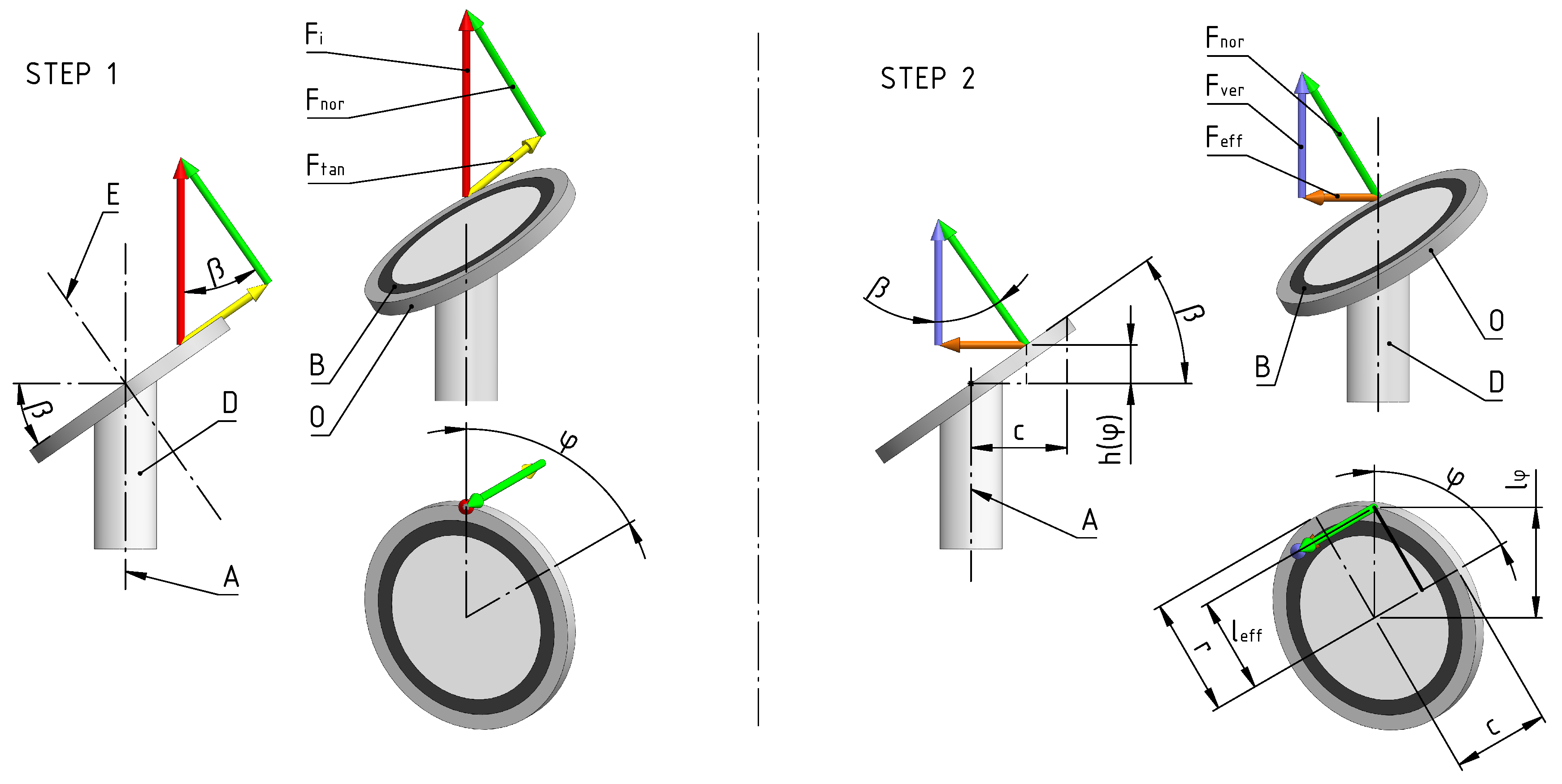
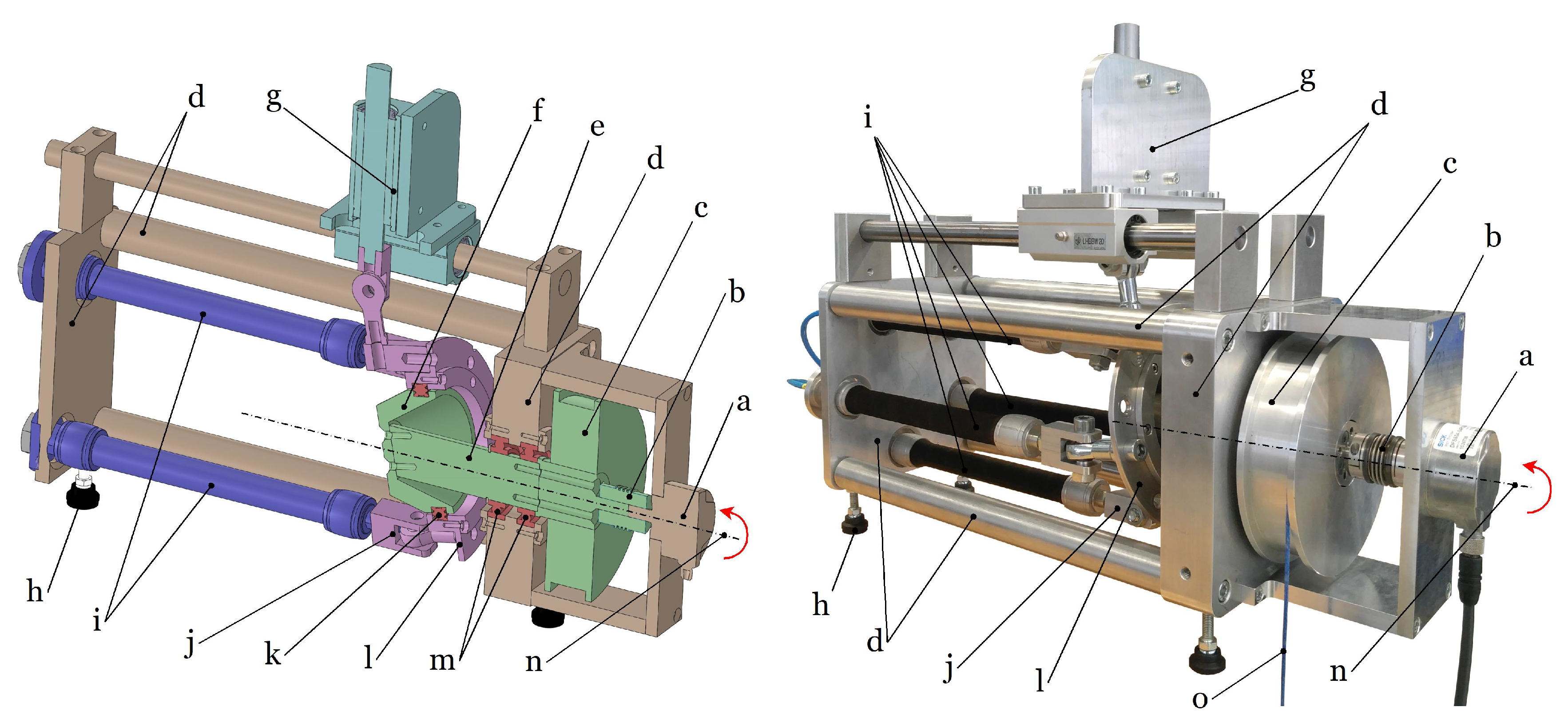
In Figure 2, a schematic of the force transmission from $F_i$, exerted by one PAM unto the outer swash plate, to the rotation force $F_{eff}$ is depicted, while in Figure 3, a sectional view of the three dimensional computer-aided-design-model (3D CAD-model) and a picture of the realized and investigated drive unit are shown. We describe the force transfer in two steps. In step one, we split up the force $F_i$ into the tangential force $F_{tan}$ and the normal force $F_{nor}$. In step two, we split up the normal force into the vertical force $F_{ver}$ and the effective force $F_{eff}$. The tangential force is absorbed by the additional fixture, and the vertical force is absorbed by the structure. Finally, the effective force $F_{eff}$ causes a torque that results in rotary motion of the drive shaft. Additionally, we make use of a four-point bearing to pivot the outer swash plate around the drive shaft. The additional fixture, depicted in Figure 3 as g, prevents the rotation of the outer swash plate. As a result, the pulling forces of the PAMs cause a change in the orientation of the inclination angle $\beta$ of the swash plate. Finally, this change of the orientation of the swash plate results in a rotation of the attached drive shaft.

The mechanical structure of the drive unit is designed to prove the operating principle and to be durable and stiff to ensure accurate measurements. As a result, the drive unit is bulky and heavy but serves the purpose of experimental testing well. The mechanical design, the pneumatic, and the electronic control setup, as well as the theoretical calculation and the measurement of the static torque distribution, are described in [3]. Moreover, we characterized the properties like adjustable stiffness and the general capability to perform high-precision positioning in the aforementioned paper.

2.2. Pneumatic Setup and Electronic Control System

We use proportional valves (FESTO, VPPM-6L-L-1-G18-0L6HV1P-S1) to set the air pressure in the PAMs to the level given by the control system. The pressure in each PAM is controlled by one corresponding proportional valve. The pneumatic control scheme is depicted in Figure 4.

One out of three different predefined pressure controller modes has to be chosen in the proportional valves. All results in the present work are obtained using the universal control behavior (middle setting) of the valves. We use a modular programmable logic controller (PLC) to operate the system. The PLC control comprises the EtherCAT coupler and several input and output terminals. The exact terminals used in the PLC are listed in Appendix A in

Table A3. Types and quantity of terminals used in the PLC control.

Pos. No.	Quantity	Name	Function
1	1	EK 1101	EtherCAT coupler
2	3	EL 4002	analog output interface
3	3	EL 3162	analog input interface
4	1	EL 5101-0010	incremental encoder interface

. The PLC is linked via the EtherCAT coupler to a control PC. We used Beckhoffs TwinCAT 3 software to write the program code for the control of the system.

2.3. Laboratory Test Stand

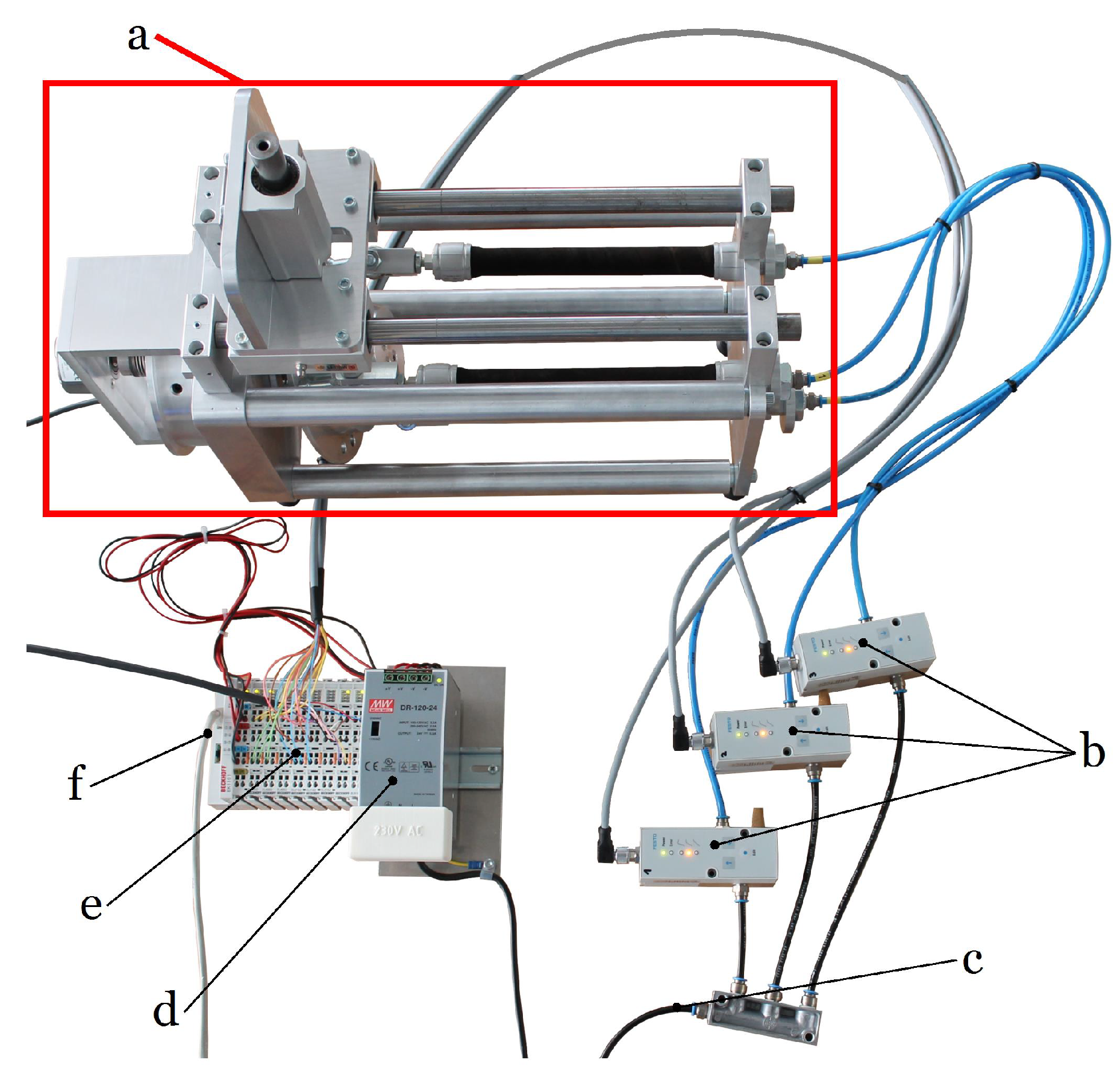
In Figure 5, an overview of the investigated laboratory test stand is depicted. This laboratory test stand is used throughout the present work to investigate the different control approaches. To ensure comparability between the different control approaches in this paper, the configuration of the drive unit is always the same. Throughout this work, we use the configuration with the inclination $\beta ={12}^{\circ }$ and $n=3$ PAMs. All parameters and symbols that we use within this paper are listed and explained in

Table A4. Specification of all further parameters and symbols used in this paper.

Parameter	Parameter Description	Value	Unit
${\phi }_{set}$	set-point value	varying	degree
$M_{total}$	controller output	varying	Nm
$M_i$	torque of muscle i	varying	Nm
$F_i$	force of muscle i	varying	N
$p_{i,real}$	pressure output of valve i	varying	Pa
$F_{i,real}$	real force of muscle i	varying	N
${\phi }_{real}$	real position	varying	degree
$\phi$	measured position	varying	degree
${\phi }_i$	position with offset	varying	Pa
A	rotary axis	-	-
B	four-point bearing	-	-
c	semi-minor axis of projected ellipse	-	-
D	swash plate	-	-
E	rotary axis of outer swash plate	-	-
O	outer swash plate	-	-
$F_{nor}$	normal force of the PAM	varying	-
$F_{tan}$	tangential force of the PAM	varying	-
$F_{ver}$	vertical force component of $F_{ver}$	varying	-
$F_{eff}$	horizontal force component of $F_{nor}$	varying	-
u	input to system, controller output	varying	Nm
y	output of system	varying	degree
$p_i$	pressure in muscle i	varying	Pa
$L_i\left({\phi }_i\right)$	Length of muscle i	varying	mm
$\gamma$	current contraction of muscle	varying	mm
${\gamma }_a$	average contraction of muscle	$rsin\left(\beta \right)$	mm
$h\left(\phi \right)$	variation around ${\gamma }_a$	varying	mm
d	unutilized value of DQZ-mapping	varying	-
q	output of controller	varying	Nm
${\alpha }_t$	auxiliary value of DQZ-mapping	varying	-
${\beta }_t$	auxiliary value of DQZ-mapping	varying	-
$M_{+}$	sum of all positive $M_i$	varying	Nm
$M_{-}$	sum of all negative $M_i$	varying	Nm
t	time	varying	s
$w\left(t\right)$	trajectory	varying	degree
${\phi }_0$	starting point of trajectory	varying	degree
${\phi }_T$	ending point of trajectory	varying	degree
T	end of time-frame of trajectory	varying	s
$a_i$	parameter for trajectory w	varying	-
N	parameter of polynomial of trajectory	2	-
K	control-parameter	0.016	-
$K_1$	control-parameter	1.8	-
$K_2$	control-parameter	107.5	-
$K_3$	control-parameter	286.5	-
$T_I$	time-constant of integrator	0.5	-
$T_1$	time-constant of valves	0.0129	-
${\mathit{x}}_{\mathit{a}}$	augmented state vector	varying	-
$\xi$	integrated control-offset	varying	-
$\mathit{Q}$	weight for $x_a$	matrix	-
$\mathit{R}$	weight for u	1	-
$K_P$	control-parameter	4.5	-
$K_I$	control-parameter	15	-
$K_D$	control-parameter	1.45	-

in the Appendix A.

3. Modelling

In the first subsection, we derive the system equation which is necessary to create a controller that is suitable to operate the presented pneumatic rotary drive unit. In the second subsection, we present the model that we use to calculate the force to pressure to length relation of the PAMs.

3.1. System Equation

The basic equation for the control of any rotary drive unit is the principle of angular momentum. It is stated with respect to the center of gravity for a stationary object in which the orientation of the angular momentum is not changing as

$$J\ddot{\phi }=M_{internal}+M_{external}=M_{total},$$

(1)

with J representing the inertia tensor and $\omega =\dot{\phi }$ representing the angular velocity. $M_{total}$ is the available torque on the drive shaft, while $M_{internal}$ represents the torque generated by the pulling forces of all PAMs and $M_{external}$ represents the torque that is externally applied to the drive shaft. The internal torque corresponds to the total torque if no external torque is applied, which is the case in this paper. The internal torque depends on the current angular position $\phi$, the force of the PAMs $F_i$, the number of PAMs n used in the drive unit as well as the inclination angle $\beta$ of the swash plate. Hence, the torque can be described as

$$M_{internal}=f(\phi ,F_i,\beta ,n).$$

(2)

In [3], the torque at the shaft is described as the sum of all internal torques caused by the PAMs and follows to be

$$M_{internal}=\sum _{i=1}^n-\frac{1}{2}{F}_{i}sin\left(2\beta \right)\frac{rcos\left(\beta \right)}{\sqrt{{cos}^2\left({\phi }_i\right)+{cos}^2\left(\beta \right){sin}^2\left({\phi }_i\right)}}sin\left({\phi }_i\right),$$

(3)

with

$${\phi }_i=\phi -\frac{2\pi }{n}(i-1),i=1,\cdots ,n$$

(4)

describing the angular position for each of the PAMs. From this approach, we derive the differential equation in the state space which is then used to control the drive. The torque $M_{internal}$ is used as the input from the controller $u=M_{internal}$. Using the states

$$\mathit{x}=\left(\begin{array}{c}{x}_1\\ x_2\end{array}\right)=\left(\begin{array}{c}\phi \\ \dot{\phi }\end{array}\right)$$

(5)

the total state-space representation of the differential equation can be derived from the Equation (1) as

$$\dot{\mathit{x}}=\underset{\mathit{A}}{\underbrace{\left(\begin{array}{cc}0& 1\\ 0& 0\end{array}\right)}}\mathit{x}+\underset{\mathit{B}}{\underbrace{\left(\begin{array}{c}0\\ \frac{1}{J}\end{array}\right)}}u.$$

(6)

As a result of the construction of the drive, the only output is the position $\phi$ which leads to the output equation

$$y=\underset{{\mathit{C}}^{\mathit{T}}}{\underbrace{\left(\begin{array}{cc}1& 0\end{array}\right)}}\mathit{x}.$$

(7)

For controlling purposes, the description of the system in the Laplace-domain, i.e., the transfer function, is often useful and therefore stated here as

$$G\left(s\right)={\mathit{C}}^{\mathit{T}}{(s\mathit{I}-\mathit{A})}^{-1}\mathit{B}=\frac{1}{J{s}^2}.$$

(8)

with the Laplace-variable s.

3.2. Force to Pressure to Length Relation of the PAMs

The fourth essential block in Figure ablaufdiagramm that has to be described mathematically is the force to pressure to length relation. The force $F_i$ exerted by a PAM onto the swash plate is a function of the inflating pressure $p_i$ of the particular PAM and of the current length $L_i\left({\phi }_i\right)$ of the PAM. The length itself depends on the angular position $\phi$ of the drive shaft, hence

$$F_i=f(p_i,L_i\left({\phi }_i\right))=f(p_i,\phi ).$$

(9)

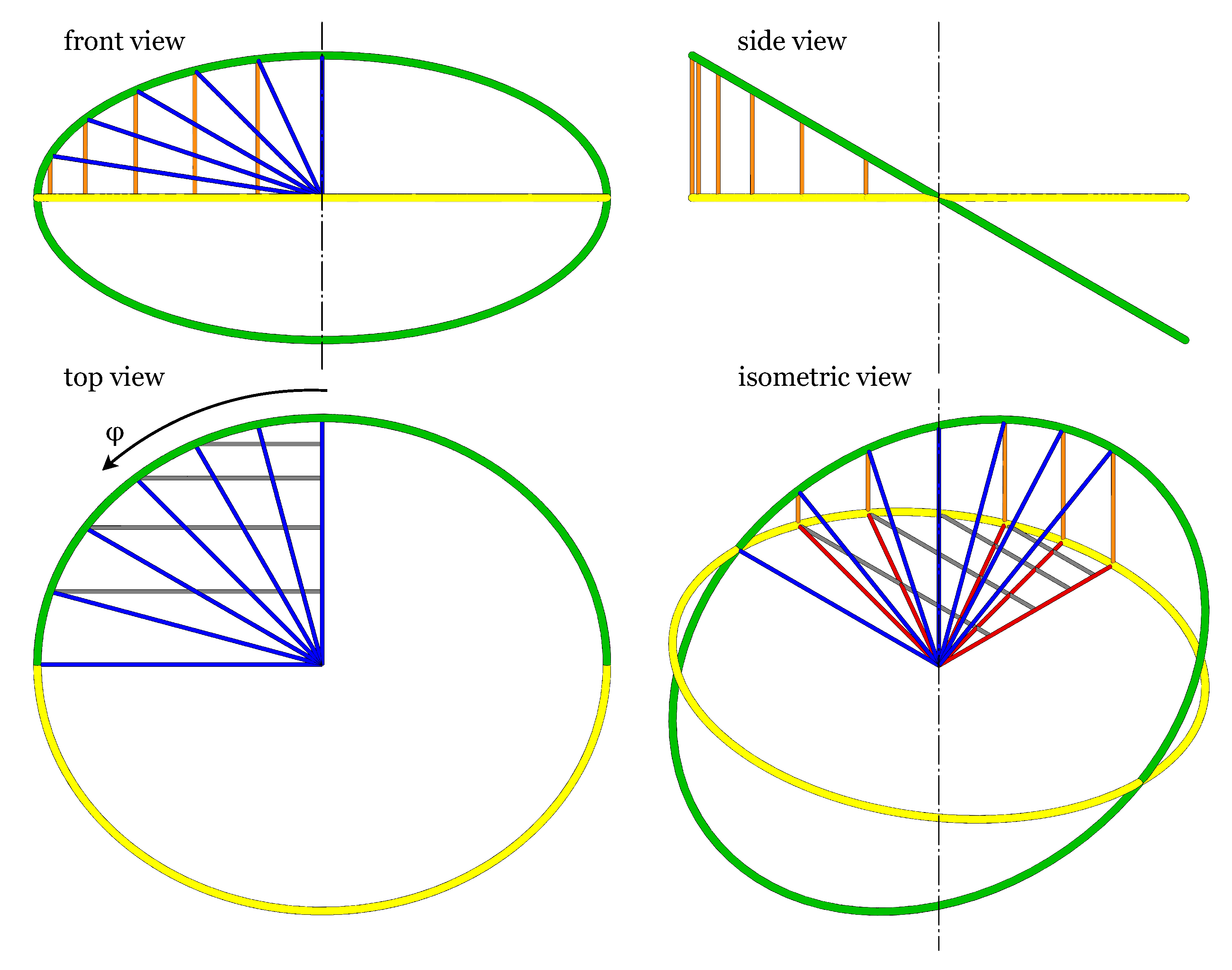
For simulation and control purposes, a good description of the length of the PAM in relation to the position is needed. To derive $L\left(\phi \right)$, we analyze the geometrical setup depicted in Figure 6. For better legibility, we only look at the first muscle and therefore set ${\phi }_i=\phi$. The other muscle equations can be obtained by using the phase offset stated in Equation (4).

From the mechanical design and the geometric dependencies presented in [3], the current length $L\left(\phi \right)$ of a PAM depends on the nominal length of the PAM $L_0$ and the current contraction $\gamma$ and is found to be

$$L\left(\phi \right)=L_0-\gamma .$$

(10)

The current contraction is the sum of the average contraction of ${\gamma }_a$, the variation $h\left(\phi \right)$, and a small and constant but not negligible offset ${\delta }_L$. With the average contraction

$${\gamma }_a=rsin\left(\beta \right)$$

(11)

and the variation

$$h\left(\phi \right)=\pm \sqrt{r^2-l_{\phi }^2},$$

(12)

the current contraction is derived to

$$\gamma ={\gamma }_a+h\left(\phi \right)+{\delta }_L=rsin\left(\beta \right)\pm \sqrt{r^2-l_{\phi }^2}+{\delta }_L.$$

(13)

Figure 6 depicts the projection of the radius r onto the horizontal plane, $l_{\phi }$ in red color. This variable is used to describe the variation $h\left(\phi \right)$ stated in (12). In [3], $l_{\phi }$ is derived to

$$l_{\phi }=\frac{rcos\left(\beta \right)}{\sqrt{{cos}^2\left(\phi \right)+{cos}^2\left(\beta \right){sin}^2\left(\phi \right)}}.$$

(14)

Due to the either negative or positive sign of the variation in Equation (12), the current length $L\left(\phi \right)$ has to be derived separately for two position sections. Finally, the description of the current length results in

$$L\left(\phi \right)=\left\{\begin{array}{cc}{L}_0-rsin\left(\beta \right)-\sqrt{r^2-l_{\phi }^2}-{\delta }_L\hfill & \mathrm{for}0\le \phi <\frac{1}{2}\pi \mathrm{and}\frac{3}{2}\pi \le \phi <2\pi \hfill \\ L_0-rsin\left(\beta \right)+\sqrt{r^2-l_{\phi }^2}-{\delta }_L\hfill & \mathrm{for}\frac{1}{2}\pi \le \phi <\frac{3}{2}\pi .\hfill \end{array}\right.$$

(15)

The real parameters of all the above-mentioned variables are specified in Appendix A in

Table A1. Specification of characteristic parameters of the laboratory test stand.

Parameter	Parameter Description	Value	Unit
n	number of PAMs	3	quantity
$\beta$	inclination angle	12	degree
r	radius	75	mm
$L_0$	nominal length of PAM	200	mm
J	inertia tensor	3,042,843	$\mathrm{g}·{\mathrm{mm}}^2$
${\delta }_L$	PAM offset	1	mm

. The relation between exerted force, applied pressure, and the current length of a PAM is called force to pressure to length relation in Figure 1. This relation is now used to calculate the pressure which has to be applied to the PAM to generate the desired force. We did not experimentally characterize our PAMs regarding the force–pressure–length relation, since such experiments have already been conducted as mentioned in Section 1.2. We use the tool “MuscleSIM” from Festo to generate a data set that describes the force to pressure to length relation for the PAMs used in the present work. The obtained data set specifies the force exerted by the PAM for different contractions (0, 5, 10, 15, 20, 25 mm) and pressures (100, 200, 300, 400, 500, 600 kPa). The general approximation approach is described in detail in [25]. The data set which is used to generate the model of the PAM can be found in Appendix A,

Table A2. Data set specifying force, F [N], pressure, p [kPa], length, L [mm] and contraction $\gamma$ [mm] for the PAMs.

$\mathit{L}\left(\mathit{\phi }\right)$	$\mathit{\gamma }$	p = 0	p = 100	p = 200	p = 300	p = 400	p = 500	p = 600
200	0	0	271.2	541.7	811.1	1078.8	1344.1	1606.5
195	5	−140.4	104.4	348.3	590.8	831.3	1069.5	1304.9
190	10	−198.1	21.9	240.8	458.1	673.5	886.5	1096.7
185	15	−224	−27.2	168.3	362	553.8	743.3	930
180	20	−236.8	−69.1	111.5	283.2	452.9	620.2	785
175	25	−244.5	−90.3	62.4	213.3	362.2	508.9	653

. The approach renders linear relations between the pressure $p_i$ and the force $F_i$

$$F_i=c_1{p}_i+c_2.$$

(16)

The offset $c_2$ is derived by plotting the relation between contraction $\gamma$ and the theoretical force at zero pressure which results in an approximation

$$c_2=0.00143286{\gamma }^4-0.104571{\gamma }^3+2.93755{\gamma }^2-40.2697\gamma$$

(17)

with $\gamma$ in mm. The slope $c_2$ is approximated in a similar fashion by looking at the slopes of the different linear relations and plotting them over the contraction $\gamma$ which renders

$$c_1=0.000306786{\gamma }^2-0.0548725\gamma +2.67668.$$

(18)

with $\gamma$ in mm.

The model in Equation (16) finally describes the PAM with regard to the relation between exerted force, applied pressure, and current contraction. The inputs in Equation (16) are $\gamma$ in mm, p in kPa, and the output is F in N. However, the described model can still return negative values for F, although the PAMs can only exert a positive pulling force. This implies that all negative values for F have to be set to zero

$$\forall p_i,\gamma :F_i(p_i,\gamma )<0\Rightarrow F_i(p_i,\gamma )=0.$$

(19)

Note that the contraction $\gamma$ only depends on the position $\phi$ of the drive shaft in terms of the length L($\phi$) stated in Equation (12).

4. Torque Mappings

As mentioned above and depicted in Figure 1, the controller sets the torque $M_{internal}$ that has to be mapped onto the different muscles. To realize the first torque mapping, we adopt the standard torque mapping used in field-oriented-control to our drive unit. The second torque mapping that we present is a simple linear approach while the third torque mapping, the simulated mapping, is derived directly from the characterization of the mechanical design. Finally, the fourth presented torque mapping is a slightly modified version of the simulated mapping with customized zero-crossing regions.

4.1. DQZ Torque Mapping

The first approach to map the given torque onto the three actuator system is to transfer the field-oriented-control approach from electric motors to this pneumatic system. This approach makes use of the combination of two transformations, the Park- and the Clarke-transform and is often also called direct-quadrature-zero transformation, or DQZ transformation, see [22,23,24]. The torques $M_1,M_2$, and $M_3$ are generated by the pulling forces of the PAMs. The relation between the force of a PAM and the respective torque on the drive shaft is stated in Equation (3). The main idea is to map two vectors of a rotating system onto three vectors of a static one. In the first step, the Park-transformation is used to transform the rotating d/q-system into the static ${\alpha }_t$/${\beta }_t$-system. Although being used in different applications, in the present application it is reduced to the rotation matrix

$$\left(\begin{array}{c}{\alpha }_t\\ {\beta }_t\end{array}\right)=\left(\begin{array}{cc}cos\left(\phi \right)& -sin\left(\phi \right)\\ sin\left(\phi \right)& cos\left(\phi \right)\end{array}\right)\left(\begin{array}{c}d\\ q\end{array}\right).$$

(20)

In the second step, the Clarke-transformation maps the static two-dimensional system onto the three muscle phases fixed to the drive. Here, the geometric relations, i.e., the installation angles between the different muscles, are used. The resulting mathematical equation is the so-called inverse Clarke-transformation

$$\left(\begin{array}{c}{M}_1\\ M_2\\ M_3\end{array}\right)=\left(\begin{array}{cc}1& 0\\ -\frac{1}{2}& \frac{\sqrt{3}}{2}\\ -\frac{1}{2}& -\frac{\sqrt{3}}{2}\end{array}\right)\left(\begin{array}{c}{\alpha }_t\\ {\beta }_t\end{array}\right).$$

(21)

The value q is used as the torque $M_{internal}$, i.e., $q=M_{internal}$, while d is an electric value which can be neglected in our application. All of this results in a first approach to map the internal torque dictated by the controller onto the three different muscles.

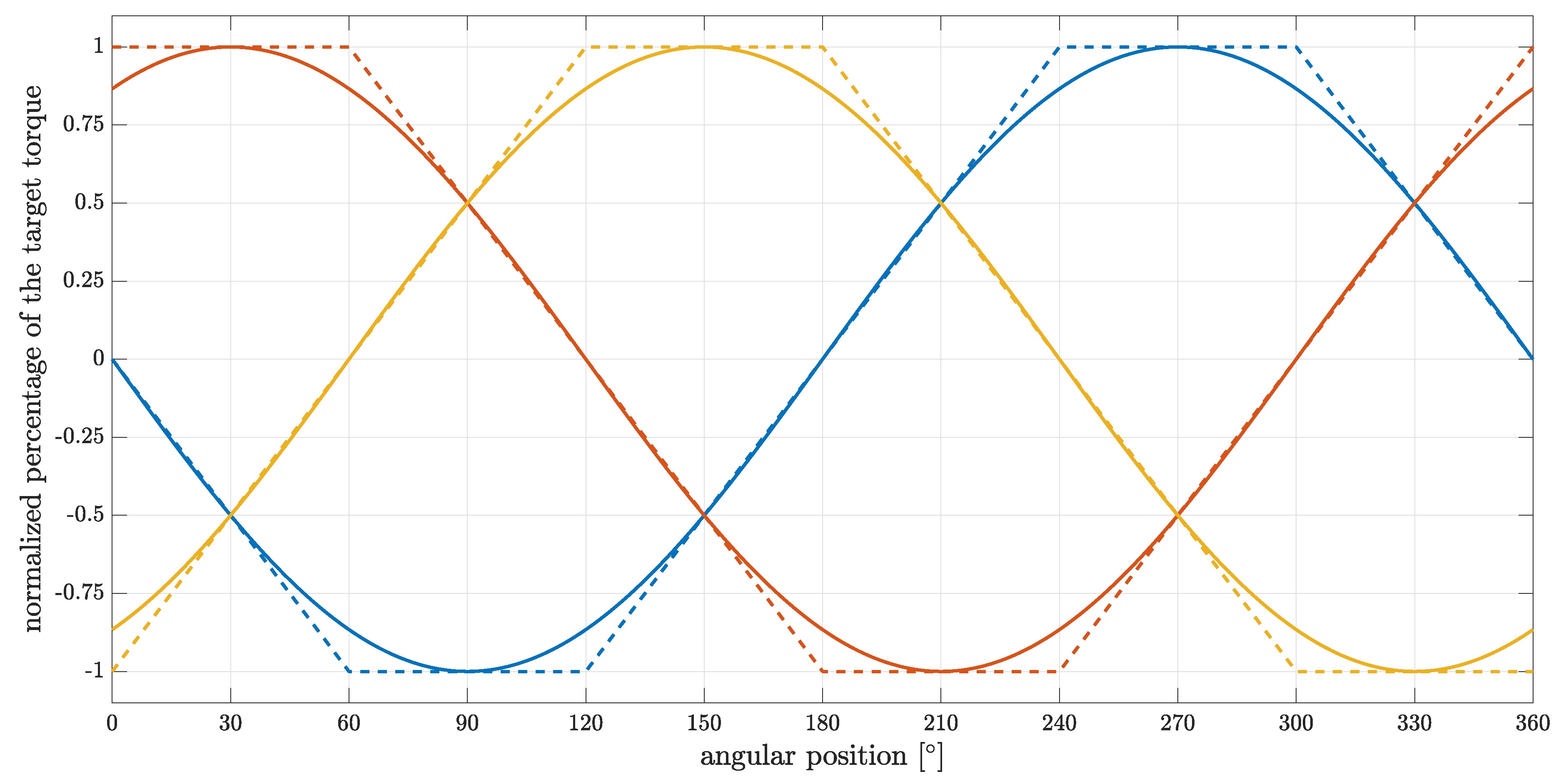
These two transformations combined result in a proportional mapping for each muscle and can be calculated for every position. The amplitude is scaled by the maximum possible torque so that a proportional value of 1 equals $M_{internal}$, as can be observed in Figure 7.

4.2. Linear Torque Mapping

The mapping resulting from the DQZ transformation relies on a drive with uniformly distributed actuators that exert both pulling and pushing forces. Since the PAMs used in this work can only exert a pulling force, the DQZ transformation can be applied but it is not perfectly suitable to work with the presented drive unit. Thus, as can be seen in Figure 7, the torque mapping using the DQZ approach is wrong in areas where only one muscle can apply torque in the desired direction. In these areas, the torque mapping has to be weighed to one. Hence, in some areas, less than the needed torque is exerted onto the drive shaft when the DQZ transformation is used to execute the torque mapping. Therefore, we created a simple linear torque mapping to correct this. In this mapping, areas where a single PAM has to account for the torque $M_{internal}$ are weighted to be one. The transitions between these areas, where only single PAM is effective, are approximated linearly. The linear torque mapping is depicted in Figure 7, together with the DQZ torque mapping described above.

4.3. Simulated Torque Mapping

The linear torque mapping does improve the areas in which a single PAM causes $M_{internal}$, but it is not a sufficient approximation of the nonlinear static torque distribution created by the behavior of the PAMs and the geometric relations in the investigated drive unit. To account for these nonlinearities, we created a mapping based on the model of the static torque distribution of the drive unit. The equations to model the static torque distribution as well as measurements of the same are presented in [3]. The main idea is to derive the percentage $x_i$ of one PAM’s torque $M_i$ to the overall torque M at the maximum pressure level for each PAM at all positions. This results in a very good approximation for all pressure levels. At each position, this results in

$$x_i\left(\phi \right)=\frac{M_i\left(\phi \right)}{M_{+}\left(\phi \right)}$$

(22)

for the positive torque with the sum of all positive torques $M_{+}$ at the position $\phi$. The same can be derived for the negative torque

$$x_i\left(\phi \right)=\frac{M_i\left(\phi \right)}{M_{-}\left(\phi \right)},$$

(23)

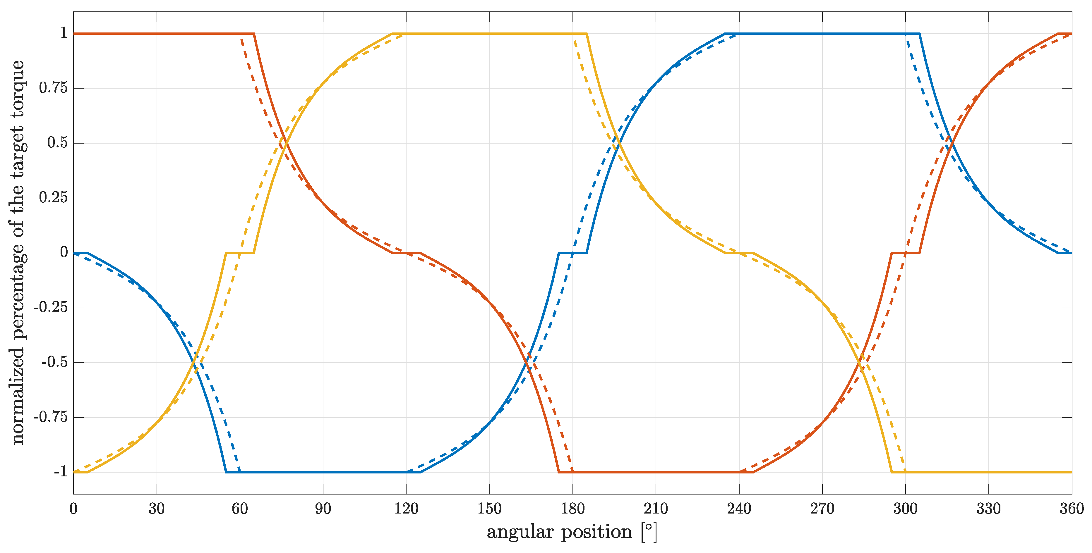
with $M_{-}$ being the sum of all negative torques. The sums $M_{+}$ and $M_{-}$ are calculated via Equation (3) by setting all $F_i=0$ that would be causing a torque in the wrong direction. Of course, the $M_i$ are caused by the $F_i$ exerted onto the swash plate. The equation for the relation between the $M_i$ and the $F_i$ is derived in [3]. The $F_i\ne 0$ apply a torque in the desired direction and are calculated by the force to pressure to length relation presented in Section 3.2. The result is a mapping which fits the potential of the PAMs; it is depicted in Figure 8.

4.4. Simulated Torque Mapping with Zero Regions

As a result of the calculation of $M_{+}$ and $M_{-}$, there are regions of the position where only one muscle can apply torque in the desired direction. Therefore, the result of $M_{+}$ and $M_{-}$ is equal to zero at several positions. Even though a division by zero does not happen in Equations (22) and (23), due to the cancellation of the $sin\left(\phi \right)$, this is still a precarious operation which we intercept by extending the zero-crossing position to a zero-crossing region in which one muscle has to account for the whole torque.

As a result, we set the other muscles to zero throughout the small area around these positions in order to not divide by zero. We chose the area to $\pm 0.5^{\circ }$ around the zero-crossing position to stay close to the original simulated mapping, but still avoid the zero-cancellation. Unfortunately, the addition of this modification also causes a slight decrease of 1.1 % of the maximum continuous torque that can be applied by the drive unit. In comparison, an area of $\pm 2^{\circ }$ would decrease the maximum continuously applicable torque by 4.67 %. This results in a slightly altered version of the simulated mapping, as can be seen in Figure 8. Here, the zero-crossing areas are displayed in an exaggerated fashion in order to make them clearly visible.

5. Control Strategies

The presented torque mappings map the internal torque $M_{internal}$ unto the different PAMs. In order to position the drive-shaft at a given set point position, the internal torque has to be specified by a controller. We implement two different control strategies which both use state space control and we compare them with regard to positioning performance. State space control means multiple states are defined and compared to the set point values in a feedback loop. This difference is then used to compute an input to the system. Hence, we present controllers which use feedback of three and four states as well as different ways of control parameter tuning. The first controller compares the closed-loop transfer function to a desired transfer function, while the second controller is based on a standard LQR-control approach. Both control strategies are well-known and described in standard control literature, see [27] for state feedback control and [28] for LQR-control.

5.1. Trajectory Generation

Depending on the implemented control approach, different controller inputs are required. The state-feedback-controller is designed to work with step inputs, while the LQR-controller is designed to follow trajectories. These trajectories are created online, as soon as the set point position is changed. Multiple parameters have to be set to realize the trajectory generation: the transition time T, the start position ${\phi }_0$, and the end position ${\phi }_T$. The trajectory $w\left(t\right)$ is generated with the help of polynomials

$$w\left(t\right)={\phi }_0+({\phi }_T-{\phi }_0)\sum _{i=N+1}^{2N+1}{a}_i{\left(\frac{t}{T}\right)}^i,t\in [0,T].$$

(24)

Additionally, $N=2$ is a parameter of the polynomial and the parameters $a_3=10$, $a_4=-15$, and $a_5=6$ ensure a smooth trajectory when adding multiple set points by making the derivatives of $w\left(t\right)$ vanish in the start and end position.

5.2. Control Strategy—Simultaneous-State-Feedback-Controller

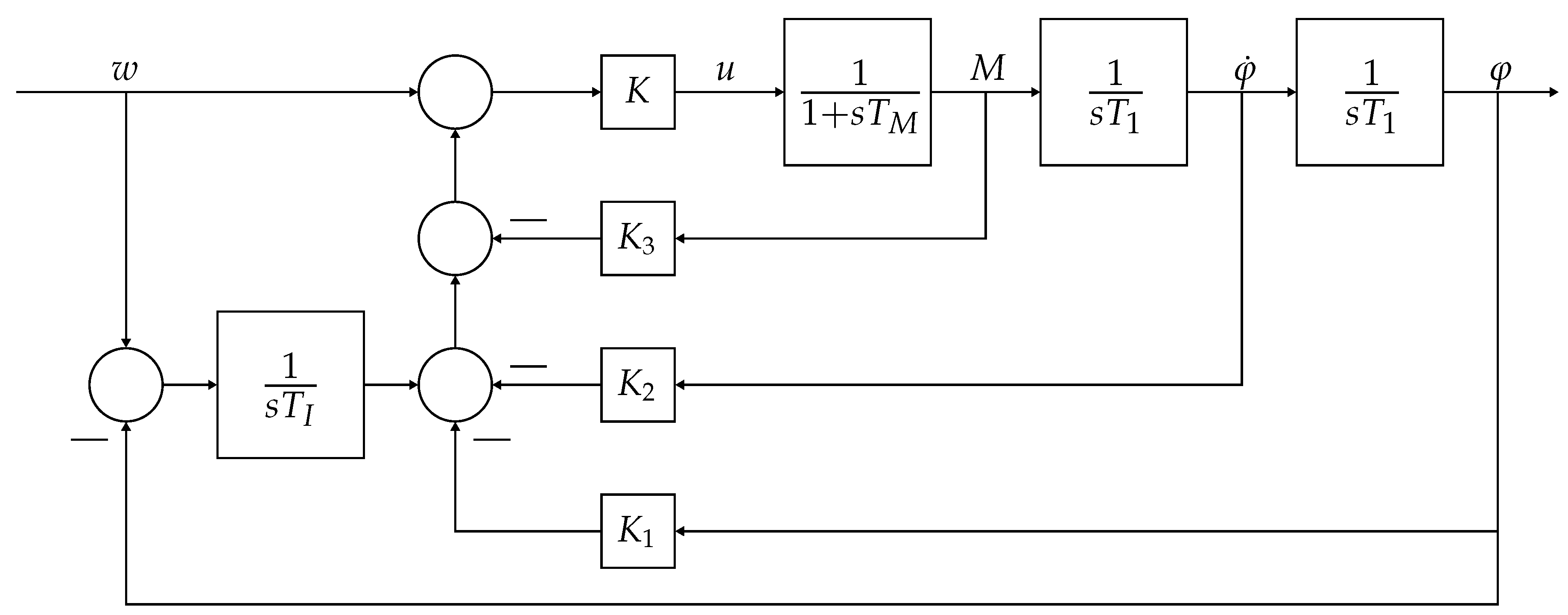
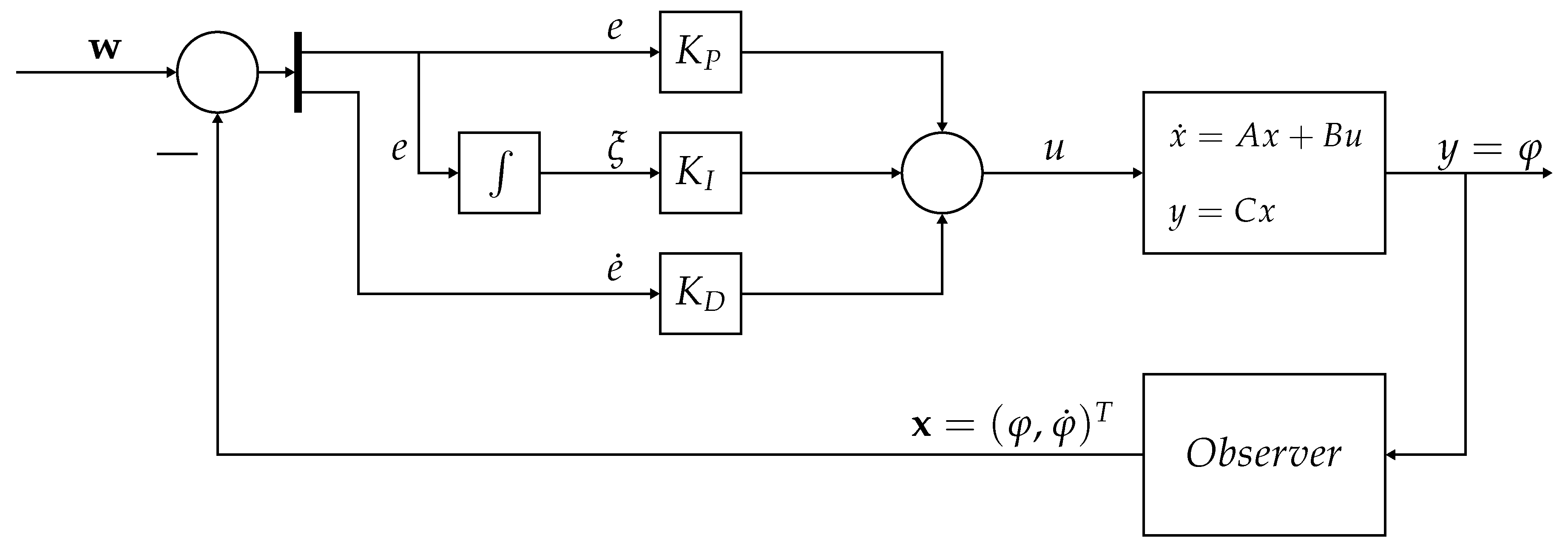
The first control approach is inspired by the control of electric drives. Its main idea is to design parameters of the control structure so that its transfer function fits a desired behavior. To achieve this, a control structure that includes the feedback of the current torque, the velocity, and the position is designed. All of these are weighed by control parameters and, in a second step, an additional integrator of the position deviation is added to form the control input to the system. The system itself is modeled as a first-order delay for the muscle response succeeded by two integrators which integrate the acceleration of the shaft resulting from the underlying principle of angular momentum.

The input of the controller is a step function. Optionally, it can be fed through the trajectory generation of Section 5.1 to create the set point values for the position and the velocity. This is then combined with the feedback signals, as shown in Figure 9, to form the control output. To derive the parameters used in the control loop in Figure 9, the transfer function $G\left(s\right)=\frac{\mathcal{L}\left(\phi \right)}{\mathcal{L}\left(w\right)}$ from the set point w to the position $\phi$ in the Laplace domain is extracted. In this first step, the integrator of the control loop is neglected. It is compared to a desired transfer function, i.e., $G\left(s\right)\stackrel{!}{=}{G}_{wanted}\left(s\right)$, which results in preliminary control parameters, but also, with [29], in the time constant $T_1=0.0129$ s. In order to remove the steady-state offset, the integrator is added which results in the transfer function

$$G\left(s\right)=\frac{\Phi }{w}=\frac{K}{K}\frac{1+s{T}_I}{1+s{T}_I{K}_1+s^2{T}_1{T}_I{K}_2+s^3{T}_1^2{T}_I(K_3+\frac{1}{K})+s^4\frac{T_1^2{T}_M{T}_I}{K}}.$$

(25)

With the help of simulations of multiple comparison transfer functions, which are defined through the parameters in

Table 1. Different parameters for the control loop, a: low-pass parameters with critical dampening, see [29], b: Bessel-low-pass with low overshoot, see [30].

	T	${\mathit{T}}_{\mathit{I}}$	K	${\mathit{K}}_1$	${\mathit{K}}_2$	${\mathit{K}}_3$
a-1	0.4	0.5	0.016	1.8	107.5	286.5
a-2	0.4	1	1.0254	1.4	69.25	272.3
b-1	0.4	2	0.016	1.2	50.13	265.2
b-2	0.4	0.5	0.889	1.8	11.78	3.234

, the remaining parameter is chosen to be $T_I=0.5$.

All choices render the transfer function stable but only a-1 is implemented.

5.3. Control Strategy—Modified-LQR-Controller

The second control strategy takes a different approach. It uses an extended control loop which results in an augmented state-feedback and it has a LQR-controller at its core to calculate the control parameters. The controller input is a set-point trajectory which is generated via the sum of polynomials in Section 5.1.

5.3.1. Control Loop

Before the controller itself can be designed, the control loop structure has to be determined. In the present case, a very precise positioning is pursued. Therefore, an integrator is used to remove the steady-state offset. As shown in Figure 10 this results in a third state variable $\xi$.

To take this into account the states of $\mathit{x}$ are augmented to

$${\mathit{x}}_{\mathit{a}}=\left(\begin{array}{c}\mathit{x}\\ \xi \end{array}\right)=\left(\begin{array}{c}\phi \\ \dot{\phi }\\ \xi \end{array}\right).$$

(26)

This results in a different representation of the model in the state space and the matrices $\tilde{\mathit{A}},\tilde{\mathit{B}}$, and $\tilde{\mathit{C}}$ are introduced

$${\dot{\mathit{x}}}_a=\underset{\tilde{\mathit{A}}}{\underbrace{\left(\begin{array}{cc}A& 0\\ -C^T& 0\end{array}\right)}}{\mathit{x}}_{\mathit{a}}+\underset{\tilde{\mathit{B}}}{\underbrace{\left(\begin{array}{c}B\\ 0\end{array}\right)}}u,$$

(27)

$$y=\underset{\tilde{\mathit{C}}}{\underbrace{\left(\begin{array}{cc}{C}^T& 0\end{array}\right)}}{\mathit{x}}_{\mathit{a}}.$$

(28)

Figure 10 depicts the control loop with the implemented LQR-controller.

5.3.2. Controller

We use a state-feedback-controller with the parameters $K_P,K_D,\mathrm{and}{K}_I$ to compute a controller output u in dependence of the augmented state, i.e.,

$$u=\left(\begin{array}{ccc}{K}_P& K_D& K_I\end{array}\right){\mathit{x}}_{\mathit{a}}.$$

(29)

In this approach, the parameters are tuned via the LQR-control approach. Its goal is the minimization of the functional

$$J(u,{\mathit{x}}_{\mathit{a}}\left(0\right))={\int }_0^t{\mathit{x}}_{\mathit{a}}^{T}Q{\mathit{x}}_{\mathit{a}}+u^{T}Rudt.$$

(30)

Here, the two matrices $\mathit{Q}$ and $\mathit{R}$ allow the prioritization of the states and the inputs. With the help of simulations and the matrices $\tilde{\mathit{A}},\tilde{\mathit{B}}$, and $\tilde{\mathit{C}}$, good values for the two matrices are found to be

$$\mathit{Q}=\left(\begin{array}{ccc}1& 0& 0\\ 0& 0.1& 0\\ 0& 0& 200\end{array}\right),\mathit{R}=1.$$

(31)

Through the LQR-theory, this results in control parameters which we slightly altered to account for differences between the real system and the simulated drive unit. This led to $K_P=4.5,K_I=15$ and $K_D=1.45$.

5.4. Comparison of the Two Control Strategies

The main difference between the two control strategies is the number of feedback states. While the first approach transfers a control approach from electric drives to the pneumatic drive unit and uses the torque as additional feedback, the second control strategy uses less feedback values and approaches the control problem under the assumption of a perfect controller-system coupling. This means that time delays are only represented as disturbances and not specifically modeled within the control loop. The second difference is the way of obtaining the control parameters. While the first controller determines them in the frequency domain via a comparison between a desired transfer behavior and the real transfer function, the second controller uses the LQR-theory to get the control parameters. Because the procedure of determining them is well-known, both strategies result in the stability of the closed loop. The last difference is the input to the two control loops. In one approach we use a step function input and in the other approach, we use a trajectory input.

6. Results

We evaluated the presented control approaches by investigating the behavior of the system in response to a step input. Two different step inputs, $0^{\circ }$ to ${90}^{\circ }$ and ${10}^{\circ }$ to ${180}^{\circ }$, were chosen to evaluate the performance of the controllers. Depending on the starting and the set-point position, the different torque mappings lead to different behavior of the drive unit. Hence, two different step inputs ensure a good comparability and reduce the risk that a combination of torque mapping and controller is used in an area in which it has a lower performance than in another section. This is the case because the transmission of the forces from the PAMs to the internal torque is non-linear. Hence, the behavior of the overall control approach strongly depends on the position areas it has to pass. Since the LQR-controller is designed to follow a trajectory, we present the behavior for both controllers when generating a trajectory first. Because the controller derived from the transfer function was originally designed to directly react to step inputs without generating a trajectory first, this behavior is also included. Moreover, we measured the step response $0^{\circ }$ to ${90}^{\circ }$ of the system with each controller and the four presented torque mappings. This leads to four hereafter presented measurement figures.

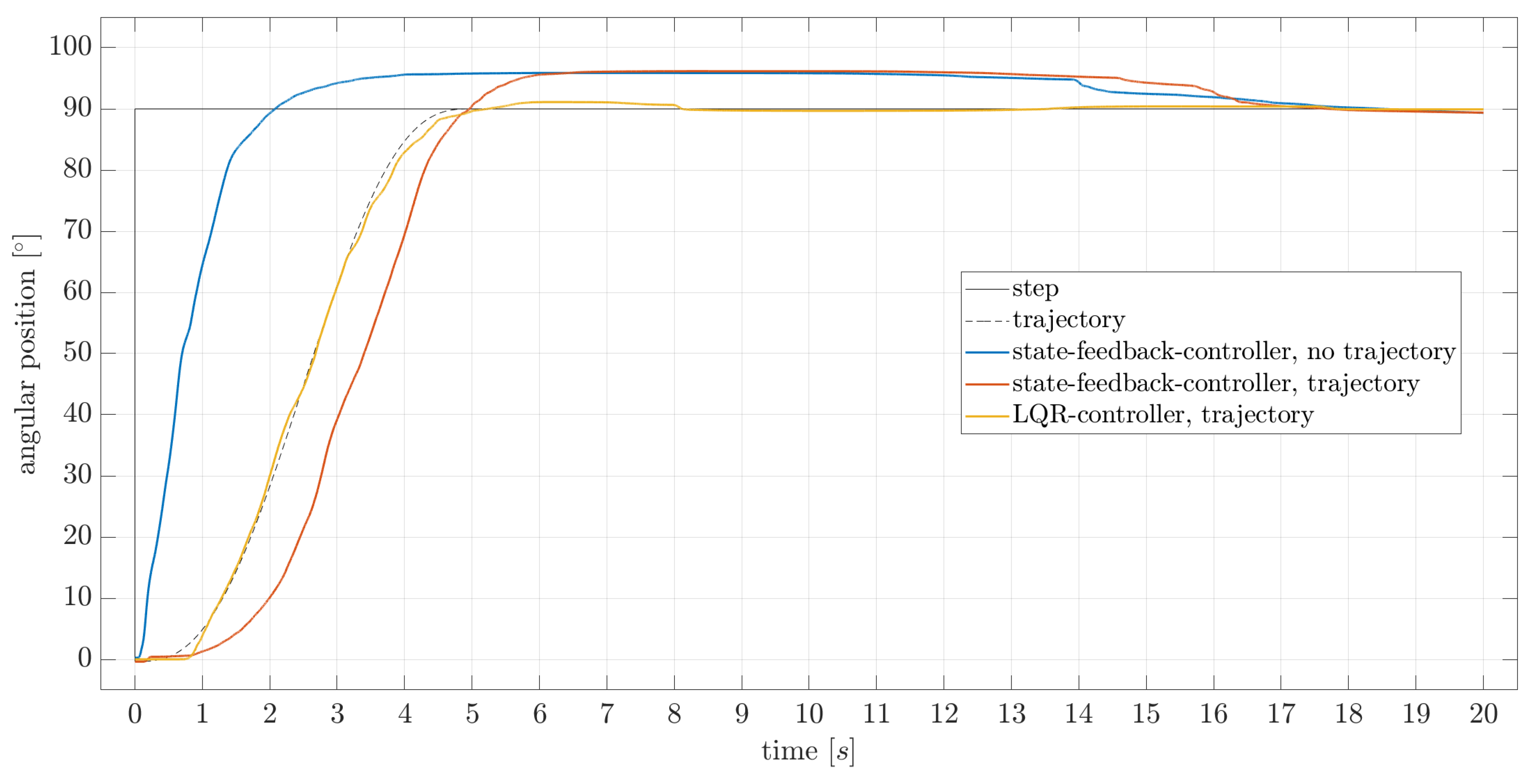
In Figure 11, the two presented controllers are compared for a step input from $0^{\circ }$ to ${90}^{\circ }$; both controllers use the mapping for which they were optimized. This ensures the best comparability. The state-feedback-controller was originally designed to work with the DQZ mapping, whereas the LQR-controller uses the improved simulated mapping with the zero-crossing areas. The step response of the state-feedback-controller is measured with and without the previously generated trajectory. Figure 11 depicts that implementing the trajectory generation changes the step response of the state-feedback-controller.

The LQR-controller shows the best performance, while the state-feedback-controller without trajectory generation responds much quicker but overshoots and needs more time to reach a steady-state.

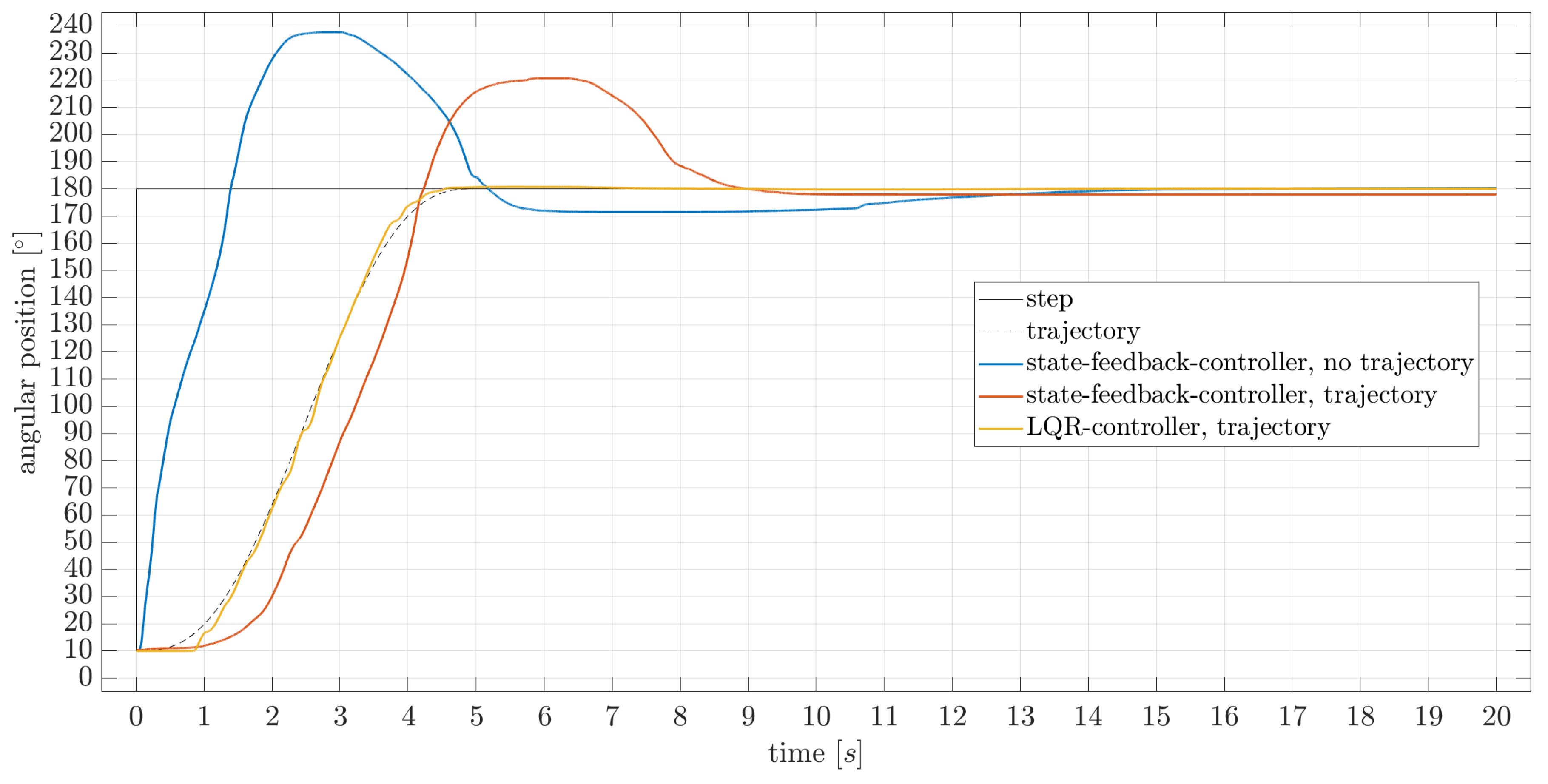
In Figure 12, the measurement is repeated for a step input from ${10}^{\circ }$ to ${180}^{\circ }$. Again, both controllers use their preferred torque mapping, i.e., the DQZ mapping for the state-feedback-controller and the simulated mapping with zero-crossing areas for the LQR-controller. Here, it is notable that the state-feedback-controller has a different step response than in the step from $0^{\circ }$ to ${90}^{\circ }$. The overshoot is stronger but the steady-state is also met quicker. This may be the case because the drive runs through the position of perfect torque transmission which results in better controller output. The response of the LQR-controller looks like the response to the previous step input. There is only a little overshoot and it also reaches the steady-state in the same time span as in the previous experiment.

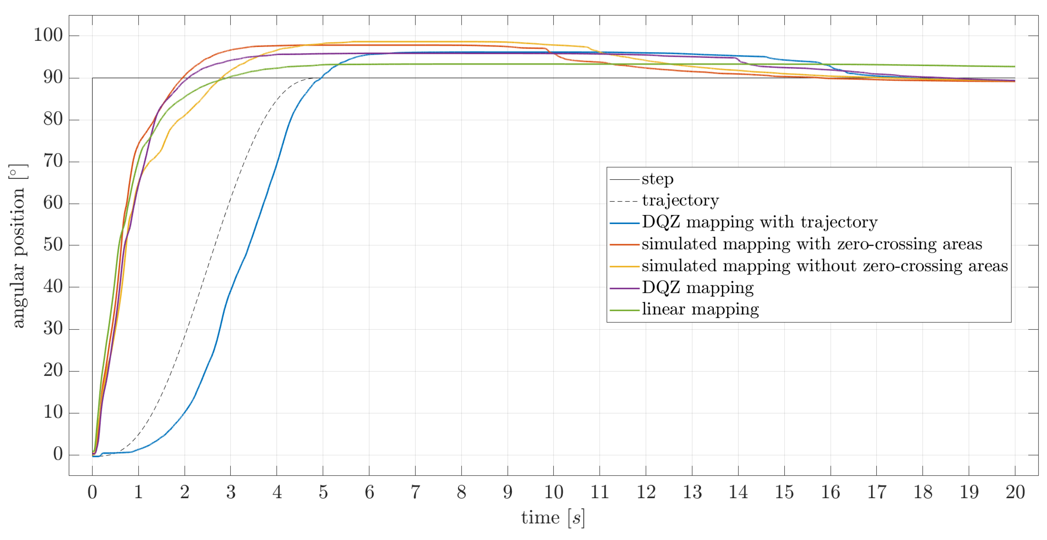
In Figure 13, the influence of the different torque mappings in combination with the state-feedback-controller is depicted. As already mentioned, the state-feedback-controller was designed to work with step inputs. Hence, we present measurements of the reaction of the system to a step input from $0^{\circ }$ to ${90}^{\circ }$. Additionally, we include the response to the trajectory input with the DQZ mapping. As depicted, the step responses vary slightly for the different mappings. Nevertheless, the addition of the zero-crossing areas results in less overshoot and quicker attainment of the steady-state in comparison to the simulated mapping without zero-crossing areas. The state-feedback-controller achieves the best overall performance in combination with the DQZ mapping. Although the linear mapping results in less overshoot, this combination takes longer to reach a steady-state. This is also the reason why we present the response to the trajectory input with the DQZ mapping, which shows a slower start of the movement, but nevertheless results in the same overshoot as the step response.

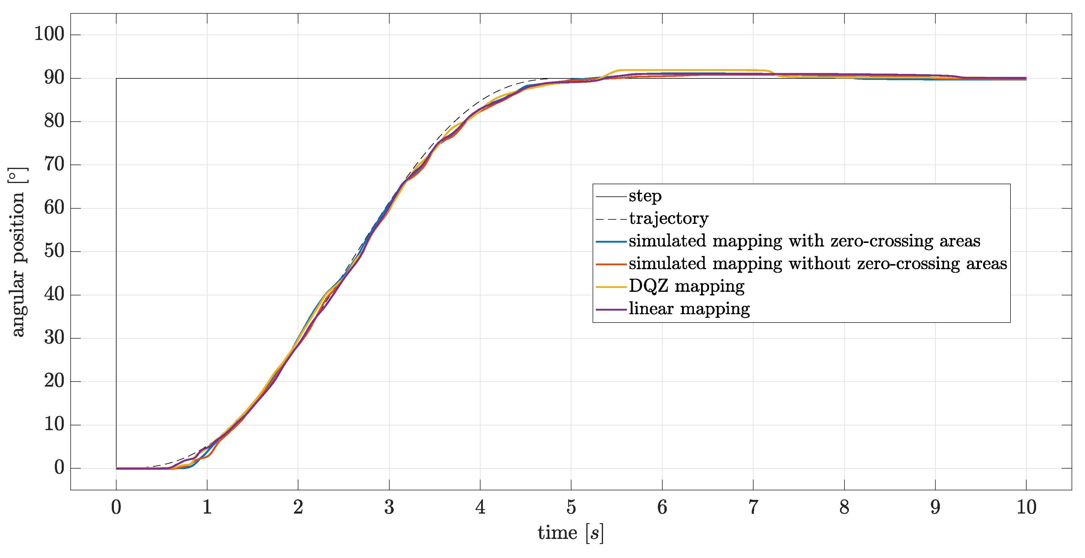
The same cannot be said for the step response of the LQR-controller in combination with the different torque mappings, depicted in Figure 14. It is obvious that all step responses are very similar except for a little overshoot performance as well as the smoothness of the trajectory. The best performance regarding position control is achieved with the simulated mapping combined with the zero-crossing areas. The linear mapping and the DQZ mapping show a greater overshoot.

7. Discussion

The presented measurements of the mechatronic system proof that the intention of the mechanical design was reached. The stick-slip phenomenon is avoided and the system can be controlled with standard control theory. Particularly the position control for a continuous 360${}^{\circ }$ motion is achieved. This enables the positioning of a robot arm with intrinsic compliance and consequently safe human-robot-collaboration. In our research, we found that the performance of the position control of the mechatronic system differs depending on the controller, the torque mapping, the starting, and the set-point position. We observe overshoot, especially for the presented state-feedback-controller in combination with the DQZ mapping, regardless of whether we generate a trajectory first or not. More experiments could help to gain a better understanding of what parameter could, in general, reduce the overshoot. Not only the overshoot, but also the time the drive unit takes until it reaches the set-point position after the overshoot takes long and should be reduced. The reaction to the step input of the LQR-controller is slower than the reaction of the state-feedback-controller, but the control performance of the LQR-controller is more consistent and the system follows the trajectory closely with less overshoot and it reaches the steady-state faster.

In comparison to the influence of the controller choice, the selection of the torque mapping does not significantly influence the behavior of the controlled system. We initially expected an improvement of the overshoot and the reaction time by using a mapping that is derived from the drive itself instead of using the existing DQZ mapping intended for electrical drives. However, the influence of the mapping is limited by the implemented controller. The state-feedback-controller showed a quicker attainment of the steady-state with the simulated mapping with zero-crossing areas in comparison to the DQZ or linear mapping. The LQR-controller, then again, does not show any significant variation of the step response when we use it in combination with different mappings. We assume that the LQR-controller reacts quicker to small changes and therefore can compensate for inaccuracies induced by the mappings that do not exactly fit to the drive unit. This assumption has to be analyzed in depth in future research.

Also subject to future research is the impact of the starting and set-point position on the performance of the controlled drive unit. On the one hand, there is no impact on the performance of the LQR-controller, but on the other hand, it changes the behavior of the state-feedback-controller significantly. This limits the usability of the presented state-feedback-controller in real control applications. The LQR-controller showed a practically identical motion throughout the working space. This behavior certainly compensates for its slower reaction times, especially when we think of using this control approach in practice.

However, the control performance of the system can be optimized, especially when the system is compared to the electronic drive units that are used in today’s robots. At this point, it is important to note that even with state-of-the-art pneumatic valves the control of the pressure in a PAM is several magnitudes slower than the speed with which electric control circuits are controlling the voltage and the electric current that is used to power electric motors. Hence, the performance of the presented position control with the pneumatic drive unit does not achieve the performance of the position control of electric drive units with similar torque but solves the problem of safe human-robot-collaboration with intrinsic compliance.

8. Conclusions and Outlook

We describe all components necessary for a complete control approach (see Figure 1) that is tailored to work with a pneumatic rotary drive that comprises three or more working chambers. Furthermore, two different control approaches are explained in detail. To map the controller output unto the PAMs used in the drive unit, we adopt the DQZ transformation known from field-oriented-control of electric motors to the available system. In contrary to the magnetic forces appearing in electric motors, the PAMs can only exert pulling forces and the system has nonlinear torque characteristics. Hence, we develop and explain three more ways to realize the torque mapping. Finally, the experimental validation shows that the combination of the LQR-controller with the simulated torque mapping with zero-crossing areas delivers the best response to a step input, independent of the starting and the set-point position.

In future research, the position control, as well as the torque mapping, could be further optimized. In the present work, only basic control theory has been applied; more advanced control strategies will surely deliver better control performance. A possible time delay and the characteristic of the pneumatic valves could be considered. Moreover, the inertia of the pressurized air has been neglected and could be modeled and included in the control approach. The complete control approaches could also be adapted to other pneumatic drive units, followed by an evaluation that will allow the comparison not only of the control approach but also of the performance of the drive units regarding their controllability. Furthermore, a control approach for force control could be realized and the behavior of the system in human-robot collaboration, especially in the case of collisions, could be investigated and compared to state-of-the-art robot systems.

References

- Stoll, J. Drehantrieb. German Patent DE 102016217198 A1, 15 March 2018. Patent pending. [Google Scholar]
- Stoll, J.T.; Pott, A. A compliant, high precision, pneumatic rotary drive for robotics. In Proceedings of the International Symposium on Robotics, VDE VERLAG GMBH, Munich, Germany, 20–21 June 2018; pp. 1–7. [Google Scholar]
- Stoll, J.T.; Schanz, K.; Pott, A. A compliant and precise pneumatic rotary drive using pneumatic artificial muscles in a swash plate design. In Proceedings of the 2019 IEEE International Conference on Robotics and Automation (ICRA), Montreal, QC, Canada, 20–24 May 2019; pp. 3088–3094. [Google Scholar] [CrossRef]
- Daerden, F.; Lefeber, D. Pneumatic artificial muscles: Actuators for robotics and automation. Eur. J. Mech. Environ. Eng. 2002, 47, 10–21. [Google Scholar]
- Kelasidi, E.; Andrikopoulos, G.; Nikolakopoulos, G.; Manesis, S. A survey on pneumatic muscle actuators modeling. In Proceedings of the 2011 IEEE International Symposium on Industrial Electronics, Gdansk, Poland, 27–30 June 2011; pp. 1263–1269. [Google Scholar] [CrossRef] [Green Version]
- Martens, M.; Boblan, I. Modeling the static force of a Festo pneumatic muscle actuator: A new approach and a comparison to existing models. Actuators 2017, 6, 33. [Google Scholar] [CrossRef] [Green Version]
- Wickramatunge, K.C.; Leephakpreeda, T. Study on mechanical behaviors of pneumatic artificial muscle. Int. J. Eng. Sci. 2010, 48, 188–198. [Google Scholar] [CrossRef]
- Hildebrandt, A.; Sawodny, O.; Neumann, R.; Hartmann, A. A cascaded tracking control concept for pneumatic muscle actuators. In Proceedings of the 2003 European Control Conference (ECC), Cambridge, UK, 1–4 September 2003; pp. 2517–2522. [Google Scholar] [CrossRef]
- Sárosi, J.; Biro, I.; Nemeth, J.; Cveticanin, L. Dynamic modeling of a pneumatic muscle actuator with two-direction motion. Mech. Mach. Theory 2015, 85, 25–34. [Google Scholar] [CrossRef]
- Ivlev, O. Modular multi-sensory fluidic actuator with pleated rotary elastic chambers. IFAC Proc. 2006, 39, 271–276. [Google Scholar] [CrossRef]
- Mihajlov, M.; Hubner, M.; Ivlev, O.; Graser, A. Modeling and control of fluidic robotic joints with natural compliance. In Proceedings of the 2006 IEEE International Conference on Control Applications, Munich, Germany, 4–6 October 2006; pp. 2498–2503. [Google Scholar] [CrossRef]
- Gaiser, I.; Wiegand, R.; Ivlev, O.; Andres, A.; Breitwieser, H.; Schulz, S.; Bretthauer, G. Compliant robotics and automation with flexible fluidic actuators and inflatable structures. In Smart Actuation and Sensing Systems; Berselli, G., Vertechy, R., Vassura, G., Eds.; IntechOpen: Rijeka, Croatia, 2012; Chapter 22. [Google Scholar] [CrossRef] [Green Version]
- Chou, C.P.; Hannaford, B. Measurement and modeling of McKibben pneumatic artificial muscles. IEEE Trans. Robot. Autom. 1996, 12, 90–102. [Google Scholar] [CrossRef] [Green Version]
- Caldwell, D.G.; Medrano-Cerda, G.A.; Goodwin, M. Control of pneumatic muscle actuators. IEEE Control Syst. Mag. 1995, 15, 40–48. [Google Scholar]
- Situm, Z.; Herceg, S. Design and control of a manipulator arm driven by pneumatic muscle actuators. In Proceedings of the 2008 16th Mediterranean Conference on Control and Automation, Ajaccio, France, 25–27 June 2008; pp. 926–931. [Google Scholar] [CrossRef]
- Tonietti, G.; Bicchi, A. Adaptive simultaneous position and stiffness control for a soft robot arm. In Proceedings of the IEEE/RSJ International Conference on Intelligent Robots and Systems, Lausanne, Switzerland, 30 September–4 October 2002; Volume 2, pp. 1992–1997. [Google Scholar] [CrossRef]
- Tondu, B. A seven-degrees-of-freedom robot-arm driven by pneumatic artificial muscles for humanoid robots. Int. J. Robot. Res. 2005, 24, 257–274. [Google Scholar] [CrossRef]
- Tondu, B.; Lopez, P. Modeling and control of McKibben artificial muscle robot actuators. IEEE Control Syst. Mag. 2000, 20, 15–38. [Google Scholar] [CrossRef]
- Martens, M.; Passon, A.; Boblan, I. A sensor-less approach of a torque controller for pneumatic muscle actuator driven joints. In Proceedings of the 2017 3rd International Conference on Control, Automation and Robotics (ICCAR), Nagoya, Japan, 22–24 April 2017; pp. 477–482. [Google Scholar] [CrossRef]
- Medrano-Cerda, G.A.; Bowler, C.J.; Caldwell, D.G. Adaptive position control of antagonistic pneumatic muscle actuators. In Proceedings of the 1995 IEEE/RSJ International Conference on Intelligent Robots and Systems, Human Robot Interaction and Cooperative Robots, Pittsburgh, PA, USA, 5–9 August 1995; Volume 1, pp. 378–383. [Google Scholar]
- Franco, W.; Maffiodo, D.; De Benedictis, C.; Ferraresi, C. Use of McKibben muscle in a haptic interface. Robotics 2019, 8, 13. [Google Scholar] [CrossRef] [Green Version]
- Binder, A. Elektrische Maschinen und Antriebe; Springer: Berlin/Heidelberg, Germany, 2012. [Google Scholar] [CrossRef]
- Akin, B.; Bhardwaj, M. Sensored field oriented control of 3-phase induction motors. Tex. Instrum. Guide 2013, 2019, 1–35. [Google Scholar]
- Schröder, D. Elektrische Antriebe - Regelung von Antriebssystemen; Springer: Berlin/Heidelberg, Germany, 2015. [Google Scholar]
- Schäffer, L. Regelung Eines Neuartigen Hochgenauen Pneumatischen Drehantriebs; Research Work; Universität Stuttgart: Stuttgart, Germany, 2017. [Google Scholar]
- Schanz, K. Weiterentwicklung Eines Regelungskonzepts und Charakterisierung Eines Pneumatischen Drehantriebs. Bachelor’s Thesis, Universität Stuttgart, Stuttgart, Germany, 2018. [Google Scholar]
- Lunze, J. Regelungstechnik 1; Springer Vieweg: Berlin/Heidelberg, Germany, 2016; Volume 11. [Google Scholar] [CrossRef]
- Lunze, J. Regelungstechnik 2; Springer Vieweg: Berlin/Heidelberg, Germany, 2016; Volume 9. [Google Scholar] [CrossRef]
- Tietze, U.; Schenk, C.; Gamm, E. Halbleiter-Schaltungstechnik; Springer-Verlag: Berlin/Heidelberg, Germany, 2016. [Google Scholar]
- Kuo, F.F. Network Analysis and Synthetis, 2nd ed.; Wiley & Sons Inc.: New York, NY, USA, 1966. [Google Scholar]
Figure 1.
Overall scheme of the control approach, input value , and output value . All blue colored boxes are described in the present paper, the grey colored box is described in [3], the red dashed box contains the computational steps, and the green dashed box contains the steps happening in the components of the realized laboratory test stand.
Figure 2.
Schematic representation of the operating principle and the force components presented in [3], drive shaft with inner swash plate D, four-point bearing B, outer swash plate O, angular position , inclination of the swash plate , rotary axis A of the drive shaft, rotary axis of the outer swash plate E. Step 1: force of the pneumatic artificial muscle (PAM) , normal force of the PAM , tangential force of the PAM , Step 2: vertical force component of : , horizontal force component of : , radius from the center of the swash plate to the force transmission point of the PAM on the outer swash plate and semi-major axis of the projected ellipse r, current projected radius , effective lever arm , semi-minor axis c of the projected ellipse, current height .
Figure 3.
Mechanical design of the investigated drive unit, (left) sectional of the 3D CAD-model, presented in [3], (right) realized drive unit, presented in [3], encoder a, coupling b, cable drum c, structure d, drive shaft e, inner swash plate f, additional fixture g, leveling foot h, PAMs i, connecting elements j, four-point bearing k, outer swash plate l, shaft bearings m, centerline of the rotary axis n, cable to attach load o, red arrow indicating the positive direction of rotation and .
Figure 4.
Pneumatic control scheme of the laboratory test stand, this figure is presented in [3].
Figure 5.
Overview of the available laboratory test stand, presented in [3], drive unit a, proportional valves b, air supply c, power supply d, PLC control e, Ethernet connection f.
Figure 6.
Front, side, top, and isometric view of the geometric relations, inclined plane of the circular swash plate colored green, projected ellipsis in the horizontal plane colored yellow, radius r from the center of the swash plate to the force transmission point of the PAM on the outer swash plate colored blue, projected radius colored red, the variation of the length of a PAM is named colored orange, effective lever arm colored grey, the rotary axis of the drive shaft is depicted as black dashed line.
Figure 7.
Torque mapping using the direct-quadrature-zero transformation (DQZ) mapping (solid line) and the linear mapping (dashed line) over angular position . Blue: PAM 1, Red: PAM 2, Yellow: PAM 3.
Figure 8.
Simulated torque mapping with (solid line) and without (dashed line) zero-crossing areas over angular position . Blue: PAM 1, Red: PAM 2, Yellow: PAM 3.
Figure 9.
Overview of control loop with torque- and state-feedback and Integrator. K, , , and are the control parameters.The set-point is w.
Figure 10.
Overview of control loop with output feedback y, observer, and augmented state . The control output is u and the control parameters are , , and . The trajectory input to the controller is w.
Figure 11.
Step responses to step input from to . The Blue and Red trajectories use the DQZ mapping, the Yellow one uses the simulated mapping with zero-crossing areas.
Figure 12.
Figure 13.
Mapping comparison for step input of to and state-feedback-controller.
Figure 14.
Mapping comparison for step input from to and LQR-controller.
© 2019 by the authors. Licensee MDPI, Basel, Switzerland. This article is an open access article distributed under the terms and conditions of the Creative Commons Attribution (CC BY) license (http://creativecommons.org/licenses/by/4.0/).
Share and Cite
MDPI and ACS Style
Stoll, J.T.; Schanz, K.; Pott, A. Mechatronic Control System for a Compliant and Precise Pneumatic Rotary Drive Unit. Actuators 2020, 9, 1. https://doi.org/10.3390/act9010001
AMA Style
Stoll JT, Schanz K, Pott A. Mechatronic Control System for a Compliant and Precise Pneumatic Rotary Drive Unit. Actuators. 2020; 9(1):1. https://doi.org/10.3390/act9010001
Chicago/Turabian StyleStoll, Johannes T., Kevin Schanz, and Andreas Pott. 2020. "Mechatronic Control System for a Compliant and Precise Pneumatic Rotary Drive Unit" Actuators 9, no. 1: 1. https://doi.org/10.3390/act9010001
Note that from the first issue of 2016, this journal uses article numbers instead of page numbers. See further details here.