Project Report

Mitigating the Climate Impact from Aviation: Achievements and Results of the DLR WeCare Project

by
Volker Grewe
1,2,*,
Katrin Dahlmann
1,
Jan Flink
3,
Christine Frömming
1,
Robin Ghosh
4,
Klaus Gierens
1,
Romy Heller
1,
Johannes Hendricks
1,
Patrick Jöckel
1,
Stefan Kaufmann
1,
Katrin Kölker
4,
Florian Linke
4,
Tanja Luchkova
5,
Benjamin Lührs
4,
Jesper Van Manen
1,2,
Sigrun Matthes
1,
Andreas Minikin
6,
Malte Niklaß
4,
Martin Plohr
7,
Mattia Righi
1,
Simon Rosanka
1,2,
Angela Schmitt
5,
Ulrich Schumann
1,
Ivan Terekhov
4,
Simon Unterstrasser
1,
Margarita Vázquez-Navarro
1,
Christiane Voigt
1,
Kai Wicke
4,
Hiroshi Yamashita
1,
Andreas Zahn
8 and
Helmut Ziereis
1
add Show full author list remove Hide full author list
1
Deutsches Zentrum für Luft- und Raumfahrt, Institut für Physik der Atmosphäre,82234 Oberpfaffenhofen, Germany
2
Delft University of Technology, Section Aircraft Noise and Climate Effects, Faculty of Aerospace Engineering, 2628 HS Delft, The Netherlands
3
Deutsches Zentrum für Luft- und Raumfahrt, Simulations- und Softwaretechnik, 51147 Köln, Germany
4
Deutsches Zentrum für Luft- und Raumfahrt, Institut für Lufttransportsysteme, 21079 Hamburg, Germany
5
Deutsches Zentrum für Luft- und Raumfahrt, Institut für Flugführung, 38108 Braunschweig, Germany
6
Deutsches Zentrum für Luft- und Raumfahrt, Flugexperimente, 82234 Oberpfaffenhofen, Germany
7
Deutsches Zentrum für Luft- und Raumfahrt, Institut für Antriebstechnik, 51147 Köln, Germany
8
Karlsruher Institut für Technologie, Institut für Meteorologie und Klimaforschung, 76021 Karlsruhe, Germany
*
Author to whom correspondence should be addressed.
Aerospace 2017, 4(3), 34; https://doi.org/10.3390/aerospace4030034
Submission received: 7 April 2017 / Revised: 12 June 2017 / Accepted: 16 June 2017 / Published: 29 June 2017

Abstract

:
The WeCare project (Utilizing Weather information for Climate efficient and eco efficient future aviation), an internal project of the German Aerospace Center (Deutsches Zentrum für Luft- und Raumfahrt, DLR), aimed at finding solutions for reducing the climate impact of aviation based on an improved understanding of the atmospheric impact from aviation by making use of measurements and modeling approaches. WeCare made some important contributions to advance the scientific understanding in the area of atmospheric and air transportation research. We characterize contrail properties, show that the aircraft type significantly influences these properties, and how contrail-cirrus interacts with natural cirrus. Aviation NO x emissions lead to ozone formation and we show that the strength of the ozone enhancement varies, depending on where within a weather pattern NO x is emitted. These results, in combination with results on the effects of aerosol emissions on low cloud properties, give a revised view on the total radiative forcing of aviation. The assessment of a fleet of strut-braced wing aircraft with an open rotor is investigated and reveals the potential to significantly reduce the climate impact. Intermediate stop operations have the potential to significantly reduce fuel consumption. However, we find that, if only optimized for fuel use, they will have an increased climate impact, since non-CO 2 effects compensate the reduced warming from CO 2 savings. Avoiding climate sensitive regions has a large potential in reducing climate impact at relatively low costs. Taking advantage of a full 3D optimization has a much better eco-efficiency than lateral re-routings, only. The implementation of such operational measures requires many more considerations. Non-CO 2 aviation effects are not considered in international agreements. We showed that climate-optimal routing could be achieved, if market-based measures were in place, which include these non-CO 2 effects. An alternative measure to foster climate-optimal routing is the closing of air spaces, which are very climate-sensitive. Although less effective than an unconstrained optimization with respect to climate, it still has a significant potential to reduce the climate impact of aviation. By combining atmospheric and air transportation research, we assess climate mitigation measures, aiming at providing information to aviation stakeholders and policy-makers to make aviation more climate compatible.

Graphical Abstract

1. Introduction

Aviation provides mobility and gives us the possibility to travel long distances in relatively short time. However, air traffic’s emission of carbon dioxide, nitrogen oxides, water vapor, particles and the formation of contrails, also contributes to anthropogenic climate change by approximately 5% in terms of temperature change [1,2,3]. Hence, it is necessary to improve the scientific understanding of the underlying atmospheric processes and to investigate and assess mitigation options, in order to cope with these climate impacts of aviation. Aircraft emissions of carbon dioxide (CO 2 ), nitrogen oxides (NO x ), sulfur oxides (SO x ), water vapor (H 2 O) and aerosols lead to concentration changes of atmospheric constituents as well as changes in the cloudiness [1,2,3,4]. These atmospheric perturbations change the radiation balance of the atmosphere and cause a radiative forcing (RF) that results in a temperature change in order to derive a new state of equilibrium of the Earth-atmosphere system.
One of the best known emissions is the greenhouse gas CO 2 . A perturbation of the atmospheric CO 2 concentration depends on the CO 2 emission strength and the removal rate of atmospheric CO 2 , which can be characterized by multiple lifetimes of about 2 up to several thousand years [4], with a mean lifetime of roughly a century. The RF estimate for the atmospheric perturbations from aviation’s CO 2 up to 2005 is 28 mW·m 2 [5].
Besides CO 2 , also non-CO 2 effects have a large impact on the RF, especially from emitted NO x and contrail induced cloudiness (CiC). NO x emissions from subsonic air traffic released in the upper troposphere and lower stratosphere enhance ozone (O 3 ) production on time scales of weeks to months. Enhanced NO x also depletes methane (CH 4 ) and causes reduced ozone production on decadal time scales. Hence, the net RF from aviation NO x depends on emission scenarios, background concentrations, the chemical rate coefficients [6] and thus the location and time of the emission [7]. The average net RF of NO x for the year 2005 is estimated to be 12.6 mW·m 2 [5]. More recent studies indicate a lower total NO x RF of around 5 W·m 2 [8,9]. However, it also has to be pointed out that some assumptions are generally made in the RF calculation for total NO x , which might lead to a too low estimate. These are the steady-state assumption of the methane response [10] and the attribution of chemical (negative) feedbacks soley to aviation, which has been questioned in the past [11].
If the humidity in the exhaust plume exceeds liquid saturation, line-shaped contrails form. Ice particles in the contrails form by freezing of liquid droplets, which condensate on soot particles and other aerosol, which are either emitted or mixed from the environment into the exhaust plume. Contrails form only under specific atmospheric conditions and often sublimate within minutes, but may persist for several hours in air masses that are supersaturated with respect to ice [12,13]. Persistent contrails can spread over large areas, eventually lose their initial linear shape, mix with other cirrus and form contrail cirrus, which look like natural cirrus, but would not exist without prior formation of contrails. The climate impact of CiC depends on their lifetime, time of day, coverage, optical thickness, temperature, albedo of the atmosphere and ground underneath and other ambient conditions [4]. Contrail cirrus clouds may also change the water budget of the surrounding atmosphere and potentially modify the optical properties of natural clouds [14,15]. The global average climate impact from CiC is determined to be 50 mW·m 2 for the year 2010 [16]. CiC is expected to warm globally, but may cool regionally during daytime over dark surfaces, such as oceans.
Further impacts arise from emitted H 2 O and aerosols, such as soot particles and sulfate droplets [17]. The estimated impact resulting from H 2 O emitted at typical subsonic flight levels is comparatively small (0.9 mW·m 2 ) due to its small influence on the atmospheric background concentration of H 2 O [18]. Whereas sulfate aerosols are estimated to have a cooling impact (−4.8 mW·m 2 , [5]) through scattering and reflecting shortwave radiation, soot particles are accounted to have a direct warming effect (3.4 mW·m 2 ) by absorbing and re-emitting thermal radiation [5]. Additionally, aerosols influence ice formation processes in the upper troposphere [19,20,21], which leads to perturbations of natural cirrus clouds and may therefore affect the climate. There is however no consensus in the literature on the magnitude of this effect and large uncertainties exist even concerning the sign of the resulting RF [22].
Commercial aviation has experienced a steady growth of travel rates over the last decades and is expected to grow approximately 4% to 5% per year in terms of passenger kilometers in the next 20 years [23]. Therefore, it is particularly necessary to reduce the climate impact per flight. This can be achieved by different mitigation options that can be divided in three different groups: technical options, operational options, and combinations of both. Technical options are, e.g., using more efficient jet engines or engines with lower NO x emissions. Emissions and climate impact can also be reduced by reducing aircraft weight or friction, by using new materials, different aircraft design or different fuels (e.g., biofuels). Beside technical options that often need a long time for introduction, there are operational mitigation options like avoiding regions in which persistent contrails will form. For operational mitigation, two different approaches can be applied: Weather dependent and climate dependent operation changes. Daytime and weather-dependent aviation climate mitigation options are presented in e.g., [24,25,26]. A different approach is to generally change operations independent of the actual weather situation as it is done, e.g., by [27], who analyzed the climate impact and cash operating costs for different flight altitudes and Mach numbers for more than 1000 routes and suggested a generally lower flight altitude and lower flight speed. This operational mitigation option can be combined with a redesign of the aircraft, as the original aircraft would be operated in off-design conditions. This redesign further increases the climate impact mitigation potential and contributes to increased eco-efficiency.
The German Aerospace Center (Deutsches Zentrum für Luft- und Raumfahrt, DLR) has launched the four year project WeCare in 2013, which is addressing both the better understanding of aviation influenced atmospheric processes, presented in Section 3 and the assessment of different mitigation options, presented in Section 4. The majority of methods and results presented here, are described in greater detail elsewhere. Here, we concentrate on an overview on the project by linking the different disciplines and referring to other publications for more details.
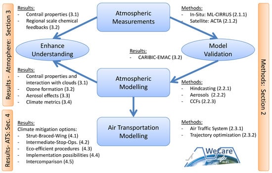
The assessment of different mitigation options requires enhancing our capabilities to investigate the underlying processes (Section 2), referring to enhancing measurement capabilities (Section 2.1) and modeling capabilities with respect to atmospheric processes (Section 2.2) and the air transportation system (Section 2.3) (see also Figure 1).
In Section 2 we first introduce measurement techniques and then modelling enhancements. The atmospheric measurement campaigns are described in Section 2.1.1 and new methods to analyze satellite data are described in Section 2.1.2. On the one hand, the obtained data will improve the understanding of atmospheric processes, e.g., aerosol-cloud interaction, on the other hand, they will help to validate atmospheric models. Here a hindcasting system (Section 2.2.1) has been established to facilitate the simulation of the atmospheric composition of past periods and to directly compare measurement and modeling results. One major area of uncertainty is the effect of aerosols on clouds, especially cirrus, which is described in Section 2.2.2. The investigation and especially the optimization of mitigation options, such as finding an aircraft trajectory with lower climate impact or an aircraft design with a lower climate impact, requires a further step, the generation of specific climate impact data. They describe the climate change per unit emission from aviation and we call them climate change functions (CCFs, Section 2.2.3, [26]). These CCFs are then used in air traffic simulations to estimate the climate impact from aviation and to optimize individual aspects of the air transportation system with respect to climate. Here we developed a 4-layer model to describe the air transportation system and to estimate future developments based on general scenario assumptions (Section 2.3.1). An important part of the description of the air traffic system is the aircraft trajectory and its optimization. Here, we developed three different optimization techniques, which are applied in different environments and tackle different aspects, such as the analysis of route changes, the impact on air traffic controller’s workload and the verification of the impact on the environment: Optimal control techniques, graph based optimization methods, and a genetic algorithm (Section 2.3.2).
In Section 3, we present results showing the impact of aviation on the atmospheric composition and on climate and further give examples of how these effects can be reduced in Section 4. We discuss results on measured and simulated contrails (Section 3.1), chemical compounds (Section 3.2), and aerosols (Section 3.3). For the assessment of mitigation options it is important to put all these effects on the same scale, which is done by climate metrics. Here, we present a way to appropriately choose such a climate metric (Section 3.4). In order to assess climate mitigation options, we established the concept of CCFs, which combine information on the atmospheric response to emissions of CO 2 , NO x , H 2 O, and the formation of contrails. We discriminate between strategic and tactical mitigation options. Strategic mitigation options concentrate on future principle changes of air traffic system such as the introduction of a new generation of aircraft (Section 4.1) or intermediate stop operations (Section 4.2). Tactical mitigation options are focusing on day-by-day changes in operations, such as avoiding climate sensitive regions (Section 4.3). Hence this discrimination focusses on the time when a decision is taken, whereas the discrimination between technical and operational measures, focuses on how the effects are mitigated. Both, tactical and strategic measures require CCFs, however, for the first climatological CCFs are applied, whereas for the latter, CCFs for the specific day, taking the meteorology of that day into account, are needed (weather-dependent CCF). Implementation measures are necessary to facilitate these mitigation options, since they often reduce aviation’s climate impact by reducing the non-CO 2 effects at the expense of additional fuel, costs and CO 2 emissions. Here we test two approaches, the closing of climate sensitive areas and the introduction of market-based-measures (Section 4.4). Finally we compare different mitigation measures (Section 4.5) and generally discuss our project layout with other projects (Section 5), before we summarize our main findings (Section 6).

2. Enhancing Capabilities: From Measurements to Modeling

Understanding the impact of aviation upon the atmosphere is the basis for assessing climate impact mitigation options. Both are complex research questions, which require a concurrent development. Here, we present progress on key aspects of aviation impacts which were achieved within the WeCare project. These achievements are based on in-situ and remote atmospheric measurements (Section 2.1) and multi-scale atmospheric modeling (Section 2.2), as well as enhancements in the modeling of the air transportation system and the integration of climate aspects (Section 2.3).

2.1. Atmospheric Measurements

2.1.1. Aircraft Experiment ML-CIRRUS

Observations of the perturbation of atmospheric components by aviation provide a data base to more accurately assess the environmental impact from aviation. To this end, the Mid-Latitude Cirrus Experiment (ML-CIRRUS) [28] with the High Altitude and Long Range Research Aircraft (HALO, Figure 2, left) was designed within WeCare to quantify atmospheric perturbations by aircraft NO x emissions and to achieve new insights into nucleation, life-cycle, and climate impact of contrail cirrus [29]. The observed variables include particle size distribution, shape, polarization, temperature and water vapour profile, chemical composition of aerosol/cloud residuals, black carbon, water vapour (total and gas-phase), NO, NO 2 , NO y , O 3 , SO 2 , HCHO, BrO, OClO (for more information we refer to [28]). Direct observations of aged contrail cirrus are rare, thus one scope of the ML-CIRRUS experiment focused on in-situ probing microphysical and radiative properties of contrail cirrus and the intercomparison to model predictions and contrail observations from space. In addition, observations of chemical species such as NO x and ozone were compared to results from a global to regional model. The instrumentation of HALO consisted of a suite of novel cloud instruments [28], a water vapor/cloud lidar [30] and an advanced aerosol, trace gas and radiation instrumentation. The aircraft observations were extended with observations from the Spinning Enhanced Visible and Infrared Imager (SEVIRI) on Meteosat Second Generation (MSG) satellite [31,32] and by numerical simulations with the Contrail and Cirrus Prediction Model (CoCiP) [15,33]. The campaign location in central Europe (Munich, Germany, Figure 2) was chosen, because it guarantees fast access to regions with high air traffic density. In spring a high abundance of both, contrails and natural cirrus is expected. Thus in March and April 2014, the HALO research aircraft performed 16 flights in contrail cirrus and mid-latitude cirrus with a total of 88 flight hours. The aircraft and the flight tracks are shown in Figure 2. Cirrus clouds were probed for more than 40 h, either with the in-situ and the remote sensing instrumentation. A comprehensive data set on natural cirrus and aircraft induced cloudiness was achieved within ML-CIRRUS.

2.1.2. Satellite Climatologies

Aging contrails are difficult to detect automatically on satellite images. The main reason is that their characteristic linear shape is lost with time, e.g., due to wind shear. However, the temporal information contained in the satellite pictures helps the observer to identify the development of an aging contrail. The automatic contrail tracking algorithm (ACTA) was developed based on this feature [35]. It starts with the known position of a linear contrail, be it by means of a contrail detection algorithm (e.g., [36]), or by means of manual selection of the contrail pixels. ACTA looks for the same contrail (a contrail with similar orientation) in the next satellite image. An edge recognition algorithm runs through the image to identify the new shape of the contrail. Based on this new information, the subsequent satellite image is processed. The ACTA algorithm can both work forward and backwards in time. This enables the analysis of the whole contrail life cycle: from any positive identification of a contrail, ACTA tracks it back to its first appearance on the satellite images and forward in time until it dissolves (Figure 3). In this case, the algorithm takes advantage of the 5 min resolution of the MSG rapid scans. This is a considerable improvement from previous contrail detection algorithms, because it allows to automatically identify a large number of cloudy pixels as anthropogenic induced cloudiness. Previously, only cloudy pixels belonging to distinct linear-shaped contrails were taken into account.
The distribution of all the contrails that are tracked using ACTA and the investigated area is shown in Figure 4. Using the ACTA algorithm a database containing a year’s worth of contrails and aging contrails was created. This database characterizes over 2000 contrails in different stages of their development, which constitutes a total of over 25,000 single contrail events. Hence this data base comprises also a good basis for a model intercomparison. Note that detection limits have to be taken into account for any model validation [37].

2.2. Atmospheric Modeling

In WeCare, enhancing the atmospheric modeling capabilities has three different aspects. First, modeling of the past atmospheric composition helps to interpret measurement data. The synergy between measurement and modeling provides a broader perspective on the data obtained and, in turn, it allows to use the data for model validation (Section 2.2.1). Second, it enables the investigation of coupled processes. These are not yet quantified and are, if at all, difficult to measure, such as the impact of aviation aerosols on clouds, especially ice clouds (Section 2.2.2). Third, atmospheric modeling is used to provide CCFs (Section 2.2.3), i.e., the relation of a local emission with its expected impact on climate. These functions are needed in air traffic system modeling to assess mitigation options.

2.2.1. Hindcasting

For an efficient use and exploitation of aircraft measurements in order to improve our understanding of aviation related atmospheric processes, comprehensive modeling of atmospheric chemistry and physics (dynamics) is performed. For this purpose, the atmospheric model MECO(n) is used, which enhances global modeling with the Earth-System Model EMAC (ECHAM/MESSy Atmospheric Chemistry, [38], please refer to the list of abbreviations for the models acronyms) by regional nesting. MECO(n) uses a modular infrastructure and combines the ECHAM global model with n-times nested COSMO models. It includes comprehensive chemistry, additional diagnostics and coupling between model domains (for more details see [39,40,41]). For the analysis of aircraft observations, a hindcast of the ML-CIRRUS campaign period is performed, by nudging model meteorology to ECMWF (European Centre for Medium-Range Weather Forecasts) reanalysis data (=Newtonian relaxation of model data to ECMWF data). Beside a detailed investigation of relevant atmospheric processes, additional simulations are performed to determine the aircraft’s impact on atmospheric composition. During the ML-CIRRUS measurement campaign in spring 2014, target regions were Europe and the North Atlantic flight corridor (NAFC), where air traffic density is high (see Section 2.1.1). The hindcast is performed using a global EMAC instance with a horizontal resolution of approximately 300 km and 90 vertical levels (T42L90MA), which includes a regional nest of approximately 25 km horizontal resolution and 61 vertical levels (0.44 ° , L61) over the European region in COSMO. In the model study we focus on the analysis of reactive chemical species, in particular NO y (sum of all reactive nitrogen species) and ozone, while using the same chemical schemes and diagnostics in both model instances.
Nudged atmospheric simulations require comprehensive preparation of input data including the provision of regular ECMWF reanalysis data and postprocessing procedures. This pre- and postprocessing of data is integrated in a software environment in order to move towards a more standardized and semi-automated input data generation. Here, the distributed integration framework RCE (Remote Component Environment) provides the capabilities to integrate simulation tools and scripts into automated data driven process chains. It allows easily coupling and executing those chain links in a graphical user interface.

2.2.2. Aerosol-Cloud Interactions

Several studies highlight the importance of aircraft-induced aerosols and their potential impact on ice formation processes in the upper troposphere (e.g., [19,20,21]). Such processes lead to the perturbation of natural cirrus clouds and may therefore affect the climate. There is however no consensus in the literature on the magnitude of this effect and large uncertainties exist even concerning the sign of the resulting RF [22].
This motivated a further extension of the aerosol model MADE (Modal Aerosol Dynamics for Europe, adapted for global applications [42]) to account for the interactions of aerosol with the ice phase in mid-level and high clouds. A new version of MADE, developed in the context of another project (MADE3, [43]), has been adopted, which allows for a better representation of aerosol mixing states in different size classes. It allows, for instance, to explicitly represent the number and mass concentrations, the size distribution, and the mixing state of insoluble particles (such as mineral dust or black carbon). They are known to act as ice nuclei for heterogeneous ice formation processes in mixed-phase and cirrus clouds [44]. Within WeCare, the new MADE3 submodel has been coupled to a new microphysical cloud module [45], which explicitly simulates aerosol-induced ice nucleation taking into account the competition between different heterogeneous ice formation pathways and the homogenous freezing of supercooled soluble aerosols [20,46].
The coupling of MADE3 with this new cloud scheme is realized in the framework of the global chemistry climate-model EMAC [47] and is now technically ready for application. Additional work however is required in this context, to optimize and evaluate the new model system, to include more constraints from experimental data that describe the ice nucleation process specifically for aviation, and to perform different sensitivity studies accounting for a plausible range of properties for aviation-emitted aerosol particles serving as potential ice nuclei. More advanced statistical methods will also need to be deployed to separate the signature of the aviation effects from the underlying noise resulting from the high model internal variability typical of these processes (e.g., [19,20]).

2.2.3. Climate Change Functions

Within the EU-project REACT4C, 5D-datasets for eight representative winter and summer days were developed, which describe the climate impact for a local emission. The first 3 dimensions represent the location of the emission, the 4th dimension the time of emission and the 5th dimension the type of emission. As type, we consider CO 2 -, NO x -, H 2 O-emissions, and a certain flown distance, latter for calculating contrail formation [26]. These datasets describes the socalled climate change functions (CCFs). The CCFs are calculated by releasing unit emissions in the model’s atmosphere, more precisely into air parcels, which are advected by the simulated wind fields and experience chemical and micro-physical processes. The resulting atmospheric changes lead to inbalances in the radiation which are then used to estimate the climate impact by using the ATR20 metric (averaged temperature response over 20 years when this re-routing strategy is applied on a daily basis, for more details we refer to [26]). Within WeCare several advancements in the CCF modeling approach were performed. We have chosen, in addition to the 8 REACT4C days, one additional day for calculating CCFs, which is one of the days of the ML-CIRRUS measurement campaign (Section 2.1.1). We have enlarged the domain (Figure 5, left) as well as the horizontal and vertical resolution (not shown). The resolution has been increased especially to consider persistent contrails which occur only in ice-supersaturated air masses. Hence, instead of using roughly a regular 15 ° by 5 ° longitude-latitude grid, we chose an irregular grid taking into account only ice-supersaturated areas, in which persistent contrails can form. We have developed an algorithm, which provides an adaptive grid. First, the potential contrail coverage (Figure 5, right) is analyzed and connected areas are identified. Second, for a given resolution, i.e., number of grid points, the mean area represented by one grid point is calculated (here: 3.24 × 10 11 m 2 or a square with 566 km side length). Third, in order to determine the location of the grid points, we divide the size of the connected area by this representative grid point area, which gives the number of grid points per connected area. These grid points are then distributed uniformly in this connected area (red crosses in Figure 5, right).
In addition to the weather dependent CCFs over Europe and USA, we have calculated global CCFs on a climatological basis for one specific aircraft. For this aircraft we first calculated the specific cruise emissions for a range of cruise altitudes and then calculated their climate impact by using the chemistry-climate response model AirClim [48,49]. Hence, the sensitivity of regional emissions on global mean near surface temperature changes is investigated by releasing specific aircraft emissions for CO 2 , H 2 O, NO x , and a given flown distance to consider contrail cirrus, at each flight level into AirClim’s emission regions. The spatial distribution of the climate impact in terms of ATR 100 (Average Temperature Response over 100 years) is normalized by the emissions at the corresponding flight level to generate climatological emission based CCFs [50]. Additionally, we have replaced the annual mean response functions of AirClim by monthly mean response functions to analyze the impact of the annual cycle. Climatological CCFs for January and July are shown in Figure 6 for aircraft specific emission indices at flight level 310 (roughly 290 hPa), exemplarily. It clearly shows a large difference in polar regions due to the annual cycle of the impact of NO x emissions on ozone. Large saturation effects over the US, Europe, and the North Atlantic Flight Corridor are visible in January. These saturation effects were previously reported, e.g., an increase in air traffic by roughly a factor in the range of 2 to 4 showed a 10% lower contrail coverage than a linear extrapolation would give [51].
The weather dependent CCFs are applied to investigate tactical mitigation measures, taking into account the actual weather situation, e.g., for eco-efficient flight procedures (Section 4.3). Whereas climatological CCFs are applied in strategic mitigation measures, e.g., new aircraft configurations (Section 4.1), principle changes in operations, such as intermediate stop operations (Section 4.2), or principle considerations on the effectiveness of implementation options (Section 4.4).

2.3. Air Traffic Modeling

The investigation of strategic and tactical mitigation options has different requirements for the representation of the air traffic system. Tactical mitigation options are more focusing on current air traffic and the optimization of current aircraft trajectories (Section 2.3.2) taking into account real weather data and related weather dependent CCFs, whereas strategic measures are applicable in more remote future. Therefore, they require a scenario forecast of demand, traffic volume, fleet composition (Section 2.3.1) and rely on climatological approaches of the impact of weather (climatological CCFs, see above).

2.3.1. Air Traffic System

To assess the climate impact of aviation including non-CO 2 effects against the backdrop of worldwide heterogeneous socio-economic growth, the future evolution of the air transportation system (ATS) has to be modeled. Within the DLR-project WeCare a modular assessment framework was developed, which is based on a 4-layer philosophy (Figure 7) for a generic description of the future passenger air traffic in networks at global scale. The four layers comprise: (1) the origin-destination passenger demand network; (2) the passenger routes network; (3) the aircraft movements network, and (4) the trajectories network [52]. The approach is implemented in the model chain called AIRCAST (air travel forecast) [53]. Due to the global network layer modeling architecture on city pair level, information on how many passengers will travel between which city-pairs in a given future year, which routes will be chosen by the passengers as well as how many aircraft and which size of aircraft will be operated on each flight segment worldwide can be provided in terms of quantitative scenarios.
As a starting point passenger demand networks are directly initialized from exogenous socio-economic scenarios [54,55]. As inputs the forecast published by Randers (2012) [56] and the five scenarios of the International Futures Global Modeling System (IFs) [57] are adapted. Passenger route probabilities are calculated based on historical ADI (Sabre Airport Data Intelligence)-data. The passenger routes network consists of two sublayers: (2a) the passenger route network and (2b) the passenger segment network. The subsequent (3) aircraft movements network with aircraft sizes and frequencies is calculated applying the DLR frequency-capacity-model FoAM (Forecast of Aircraft Movements) [58] and fleet renewal model FFWD (Fast Forward) [59]. It also consists of two sublayers: (3a) the aircraft movements network by seat categories and (3b) the aircraft movements network by aircraft type and aircraft generation.
Modeling the structural evolution of global air passenger flows and aircraft movements over time is a necessary means to quantify future shifts induced by heterogeneous growth in world regions and airline as well as passenger behavior [60]. The predicted shifts might affect the climate impact of non-CO 2 emissions substantially in the future. An early and detailed understanding of such structural changes may be strategically essential in encountering climate change appropriately. Finally, using these aircraft movements, the amount, locus and time of emissions can be computed by trajectory simulations under realistic operational conditions with GRIDLAB (Global Air Traffic Emissions Distribution Laboratory) [61] which in turn is the input to the chemistry-climate response model AirClim [48,49]; its integration is done by the RCE [62].
Since the climate impact of aviation highly depends on the amount, species, altitude, and latitude of emissions [63], a future simulation of the ATS requires a suitable geo-spatial model suite of global air traffic to develop relevant quantitative future scenarios until 2050 [64]. This way potential mitigation strategies (as described in Section 4.3 and Section 4.4) and revolutionary new concepts (as shown in Section 4.1) can be evaluated satisfyingly with respect to CO 2 and non-CO 2 effects and global aviation climate targets.

2.3.2. Trajectory Optimization

The idea of realizing routing options with a reduced climate impact requires aircraft trajectory optimization techniques. In order to be able to investigate different aspects of this problem, such as the analysis of route changes, the impact on air traffic controller’s workload and the verification of the impact on the environment, we have developed three different optimization techniques which are applied in different environments: Optimal control techniques are applied within the Trajectory Optimization Module, graph based optimization methods are used in TrafficSim, and a genetic algorithm is applied in AirTraf. The objectives when applying these models are different and hence also the model set-ups differ. For example, the analysis of current day air traffic is performed with TrafficSim, which includes routing without trajectory conflicts and air space constraints (e.g., military air space), whereas the impact of optimization strategies on the atmospheric response is performed with EMAC/AirTraf, which focusses on atmospheric modelling with a simplified air traffic simulation. However, we harmonized the underlying cost model and assumed 0.75 Euro/kg for fuel and 25 Euro/min for crew costs, based on work within the REACT4C project [26].
The Trajectory Optimization Module (TOM) allows for a continuous four-dimensional optimization of aircraft trajectories (for more details see [66]). The underlying optimal control problem has the following general form:
minimize
J t , x ( t ) , u ( t ) = c Y · Y t 0 , t f , x ( t 0 ) , x ( t f ) + c Ψ · t 0 t f Ψ x ( t ) , u ( t ) , t d t
subject to
x ˙ ( t ) = f ( x ( t ) , u ( t ) , t )
x ( t 0 ) x min , 0 ; x max , 0
x ( t f ) x min , f ; x max , f
x ( t ) x min ; x max
u ( t ) u min ; u max
p ( t ) p min ; p max
Here, x ( t ) denotes the aircraft’s state variables (position, speed, aircraft mass, and accumulated emission masses), u ( t ) denotes the aircraft’s control variables (heading angle, acceleration, and relative thrust), and p ( t ) is used to describe flight envelope constraints (pressure level, Mach number, calibrated air speed, and relative lift coefficient). The objective function J (see Equation (1)) consists of a penalty function Y , for example fuel and crew costs), which is evaluated at the initial and final point of the trajectory as well as the temporal integral over a penalty function Ψ , for example evaluating the climate impact (see also Section 4.3). Both penalty terms can be traded against each other with the corresponding scaling factors c Y and c Ψ . The optimal trajectory is obtained by identifying a control input u ( t ) which minimizes the objective function J under consideration of the dynamic constraints (see Equation (2)). The dynamic constraints consist of the aircraft’s equations of motion assuming a point-mass model with variable aircraft mass and three degrees of freedom based on Eurocontrol’s Base of Aircraft Data (BADA) 4.0 aircraft performance models [67]. Moreover, Boeing Fuel Flow Method 2 is applied in order to estimate aircraft’s emissions [68,69]. According to the problem at hand, further control (e.g., thrust limit), state (e.g., maximum speed) as well as path limitations (e.g., maximum pressure altitude) can be considered within the optimization (see Equations (3)–(7)).
Within the software module TrafficSim the optimization strategy follows a network flow model and uses Dijktra’s algorithm that respects the aircraft performance for different aircraft types based on BADA 3.9 [70]. For the network flow problem [71,72], the airspace under consideration is discretized using a network of four-dimensional nodes (latitude, longitude, altitude and time). The airspace under consideration is aligned along the direct route connection between departure and arrival airport. It is assumed that an optimal route will be close to the direct connection if fuel consumption, duration and distance are used as parameters in the objective function. In perpendicular direction to the direct route, the network forms a diamond shape as shown in Figure 8. The diamond outline reduces the runtime because the network used by the Dijksra’s algorithm stays small. The airspace under consideration is limited to the en-route segment of a trajectory and to the region that is covered by the CCF (see Section 2.2.3). The costs (in a mathematical sense, not necessarily economic) of a directed edge ( i t 1 , j t 2 ) between nodes i to j in the four-dimensional network take into account both the CCF and the flight performance of the aircraft. Taking into account the aircraft performance data already in the optimization step ensures that resulting trajectories can be followed by the corresponding aircraft. The performance of an aircraft is based on the total energy model (BADA 3.9, [70]), also taking into account wind conditions. Distance, fuel consumption and emissions are required to calculate the climate costs for an edge. Depending on aircraft’s speed and wind conditions, the duration between i and j may differ and affects t 2 . Starting from an optimization that uses optimal wind routes and avoids aviation obstacles like volcanic ash cloud regions, the optimization process is improved to calculate climate-optimal routes.
AirTraf (for a complete description see [73]) was developed as a verification platform for climate optimized routing strategies. AirTraf is a new submodel of the EMAC model ([47] see also Section 2.2) to simulate global air traffic (online) with respect to a selected routing strategy (routing option), such as optimal for wind, fuel, cost or climate, based on climate impact predictors. This platform is useful to investigate the potential for mitigating climate impact of the respective routing option.
Global flight plans (any arbitrary number of flights), Eurocontrol’s Base of Aircraft Data (BADA Revision 3.9, [70]) and International Civil Aviation Organization (ICAO) engine performance data [74] comprise the input to AirTraf. Departure times from the flightplan are checked during the simulation of the Earth-System Model EMAC and aircraft trajectories are calculated taking into account the information on the aircraft and engine performance data. The genetic algorithm (ARMOGA version 1.2.0, [75,76]) optimizes flight trajectories with respect to a selected routing option. It takes into account the local weather conditions for every flight, which are provided by EMAC, and finds an optimal trajectory including lateral and altitude changes. Fuel use and emissions are calculated by the total energy model based on the BADA methodology [77] and DLR fuel flow method [78] on the calculated trajectories. For the flight trajectory and the fuel consumption and emission calculations described above, EMAC provides local weather conditions along the trajectory. AirTraf outputs the calculated flight trajectories and three dimensional emission fields of NO x and H 2 O, fuel use, and flight distance. As an example for the output fields, Figure 9 shows the global distribution maps of the fuel use (in kg(fuel)box 1 s 1 ) for great circle (flight level at 290 hft) and flight time routing options for a typical winter day. Here, the flightplan consists of 103 trans-Atlantic flights. The results show that the flights in the time-optimal case are spread over a larger area than in the great circle case. The total amount of fuel use decreases by −5.4% for the time-optimal case [73]. The difference in fuel use between the two routing options is clearly revealed and the options are directly assessed. CCFs (Section 2.2.3), which quantify the impact of the emissions on climate change, can be used as predictors or estimates of the climate impact to optimize each individual aircraft trajectory with AirTraf. Thus, the best routing strategy for minimum climate impact will be found.
A coupling with various submodels of EMAC is straightforward and more complex routing options will be integrated: NO x , H 2 O, fuel use, contrail, CCFs [7,80,81], etc. AirTraf also enables the feedback of the calculated emissions to atmospheric processes, such as contrail and ozone formation, which provides then a verification of the climate impact reduction potential of the chosen routing strategy.

3. Aviation Effects on the Atmosphere

In the previous Section, we have discussed major measurement and modeling enhancements, which were achieved within WeCare. Here, we present new insights in the effects of aviation on the atmosphere (Section 3), and discuss options to reduce these effects in the subsequent Section 4. We have advanced both aspects in parallel: the enhancement of our capabilities and the enhancement of the understanding of atmospheric and aviation related processes. The measurement campaign ML-CIRRUS (Section 2.1.1) was performed to obtain new insights in contrail and cirrus properties (Section 3.1), validate chemistry aspects of the EMAC and MECO(n) models (Section 3.2) and derive new CCFs (Section 2.2.3). The climatological and weather related CCFs (Section 2.2.3) were combined with new air traffic system (Section 2.3.1) and trajectory optimization techniques (Section 2.3.2) to evaluate mitigation options (Section 4.1, Section 4.2, Section 4.3, Section 4.4 and Section 4.5).

3.1. Contrails

In this Section we show results on contrail properties as measured in-situ and from space during the ML-CIRRUS measurement campaign. These help to understand contrail processes, whereas satellite based remote sensing enables a more climatological approach. Further, the question arises, whether the individual contrails differ for different aircraft types [82] and different meteorological situations, which are investigated by Large-Eddy-Simulations (LES). Contrails normally refer to aircraft condensation trails, which are produced by the exhaust of an aircraft. In addition, aerodynamic contrails might form by expansion of air flowing around the aircrafts’s wings. They might also play a role, although probably a minor one. This aspect of contrails is dealt with at the end of this section.
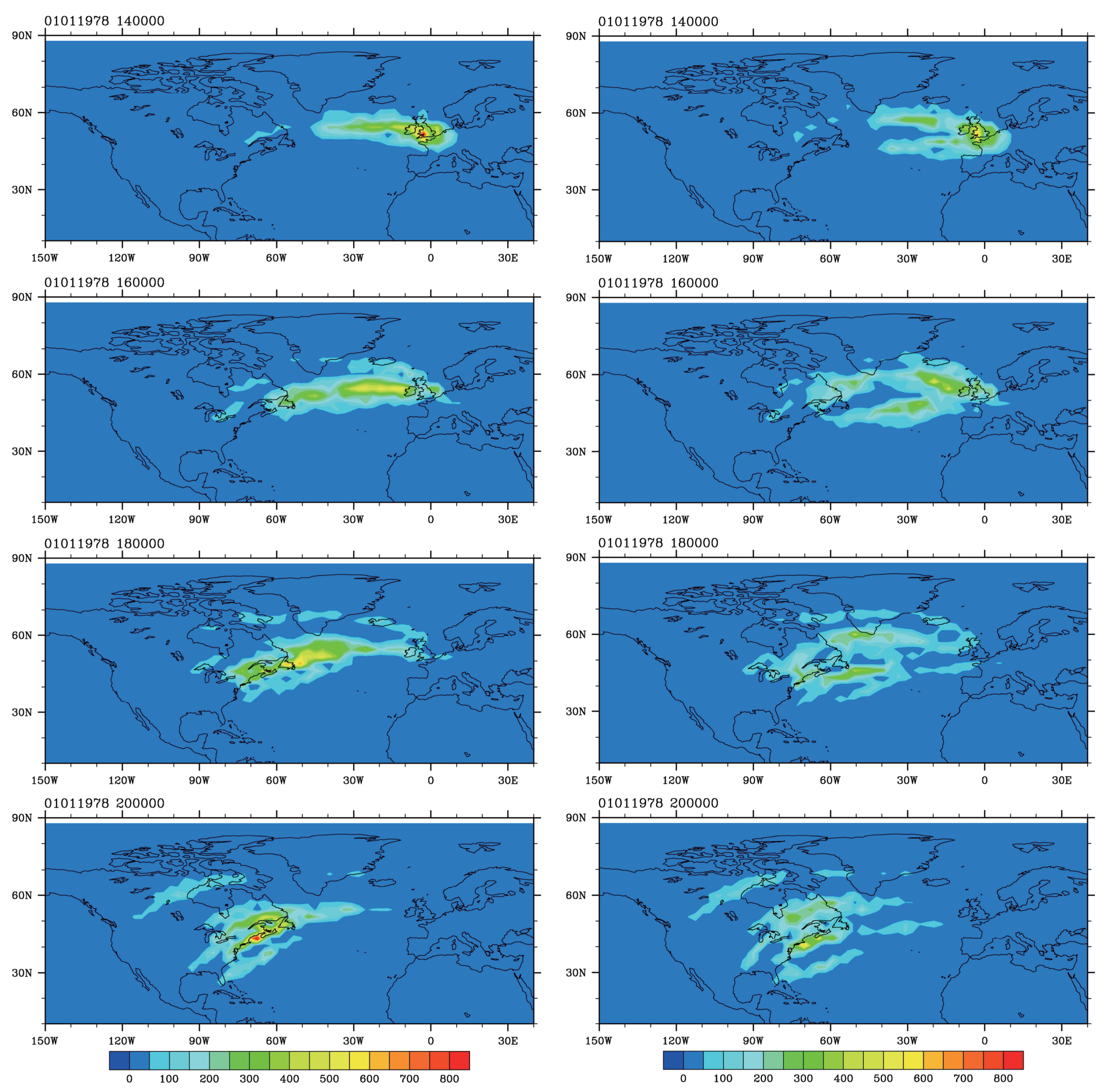
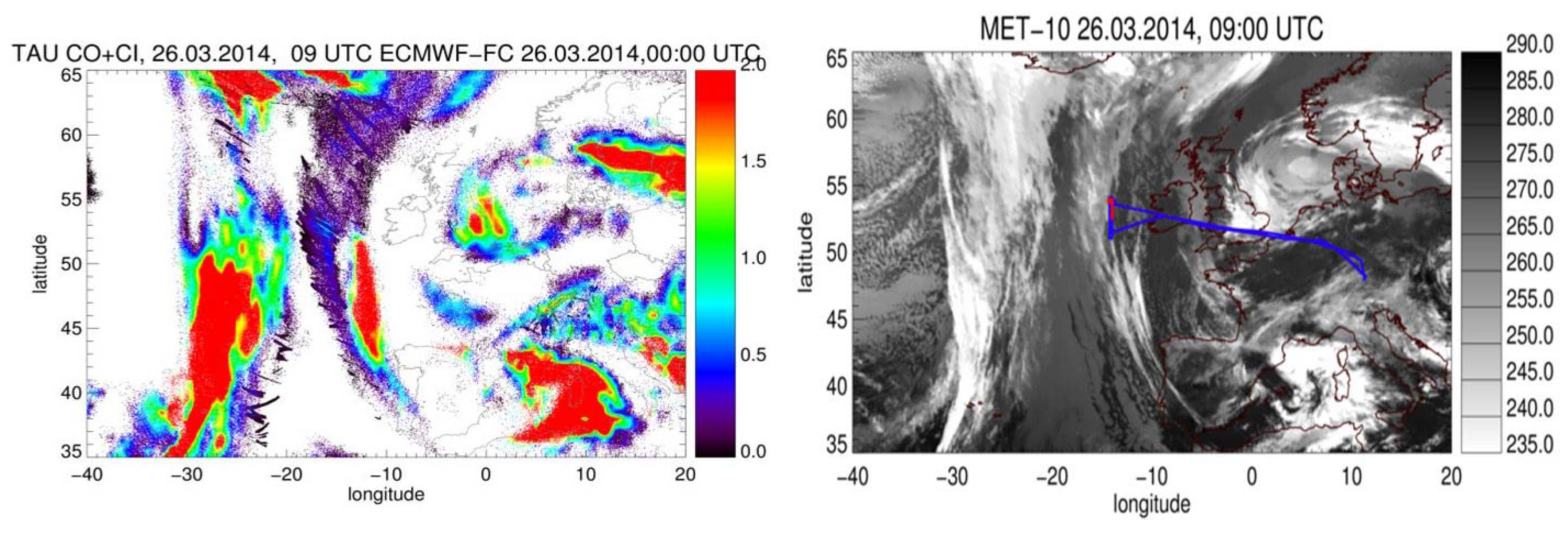
One highlight of the ML-CIRRUS mission was the frequent detection of contrail cirrus from aircraft and space (see also Figure 10, right). The occurrence of contrail cirrus was predicted by CoCiP (Figure 10, left). CoCiP has been developed to model on a global scale the lifecycle of contrail cirrus from their formation behind individual aircraft until final dissipation [33]. The model computes the contrails from all aircraft in the air space and their development to contrail cirrus. The simulated contrails evolve, taking into account relative humidity and cloud coverage from the meteorological data set by the European Center for Medium-Range Weather Forecasts (ECMWF).
During the flight on 26 March 2014, contrail cirrus were frequently probed with the in-situ instrumentation on the HALO aircraft. Simultaneous observations of nitrogen oxides [83,84] and particle number densities were used to identify contrail cirrus and to separate contrail cirrus and natural cirrus [85]. Contrails clearly show elevated concentrations in nitrogen oxides and particle concentrations [86]. From the NO y peaks, we calculate the age of the contrails [87] and discriminate between contrails and natural cirrus. (More information on NO y measurements and simulations are given in Section 3.2.) Further, we perform back trajectory and CoCiP calculations from contrail positions to identify the potential source aircraft. 
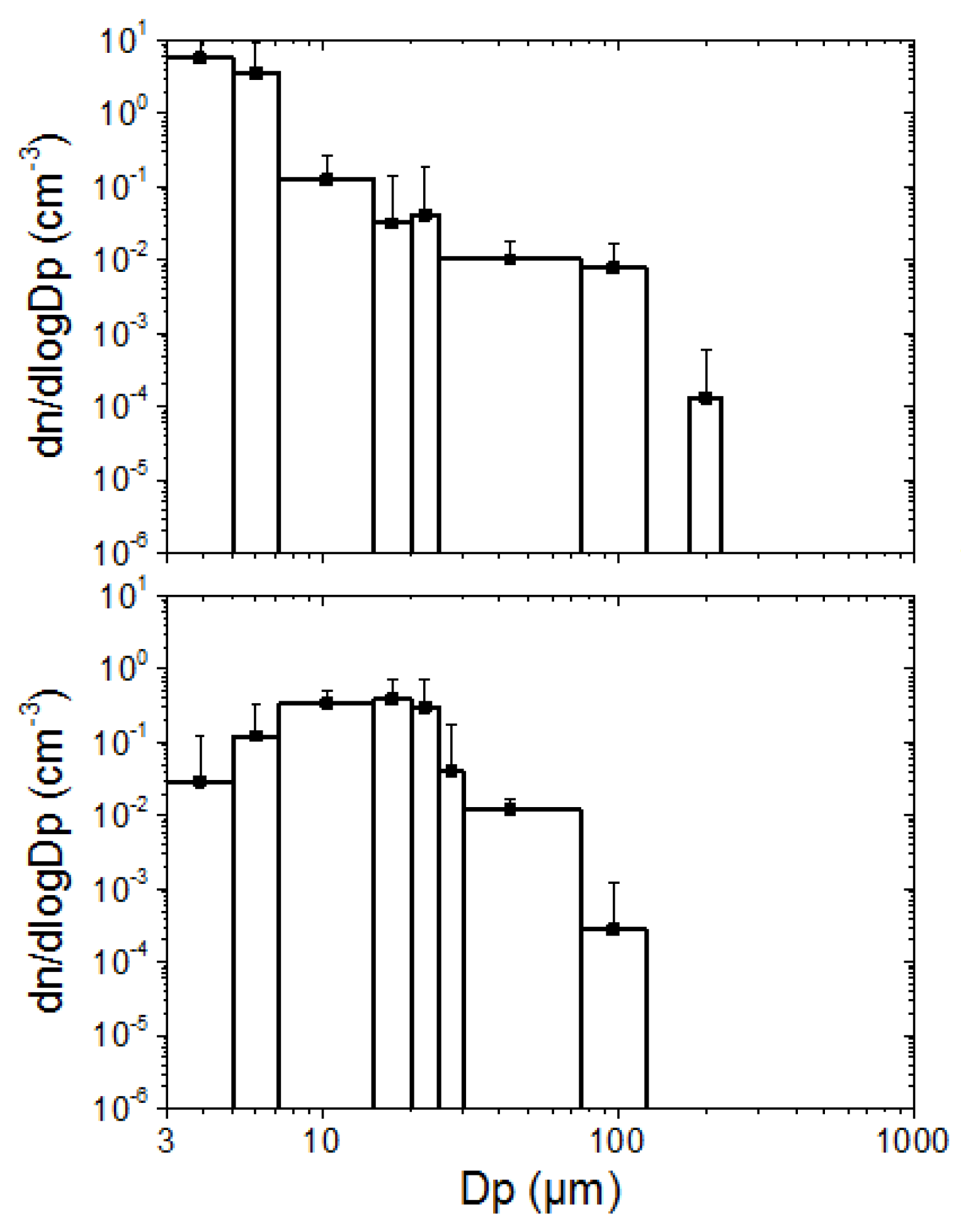
Figure 11 shows the particle size distribution in a younger and an aged contrail cirrus [28]. Trajectory calculations suggest that the contrail cirrus potentially originated from a B763 (2.6 h contrail age) and from a F900 (7.2 h age) source aircraft. Despite their age, the ice particle properties in these aged contrails still differ from natural cirrus. During aging, the ice crystals grow by uptake of water from the gas phase leading to a shift in the size distribution [88]. In addition, spreading of the contrail leads to dilution and to a decrease in ice number concentrations. Fall streaks of contrails, which originate from sedimenting ice particles are not considered here, since they cannot be identified by NO y peaks. The observations enhance the existing data base of contrail observations (e.g., [82,85,89,90,91]) as compiled by Schumann et al. [92]. The data will be used to investigate radiation extinction by contrails, and can be compared to satellite retrievals and model results.
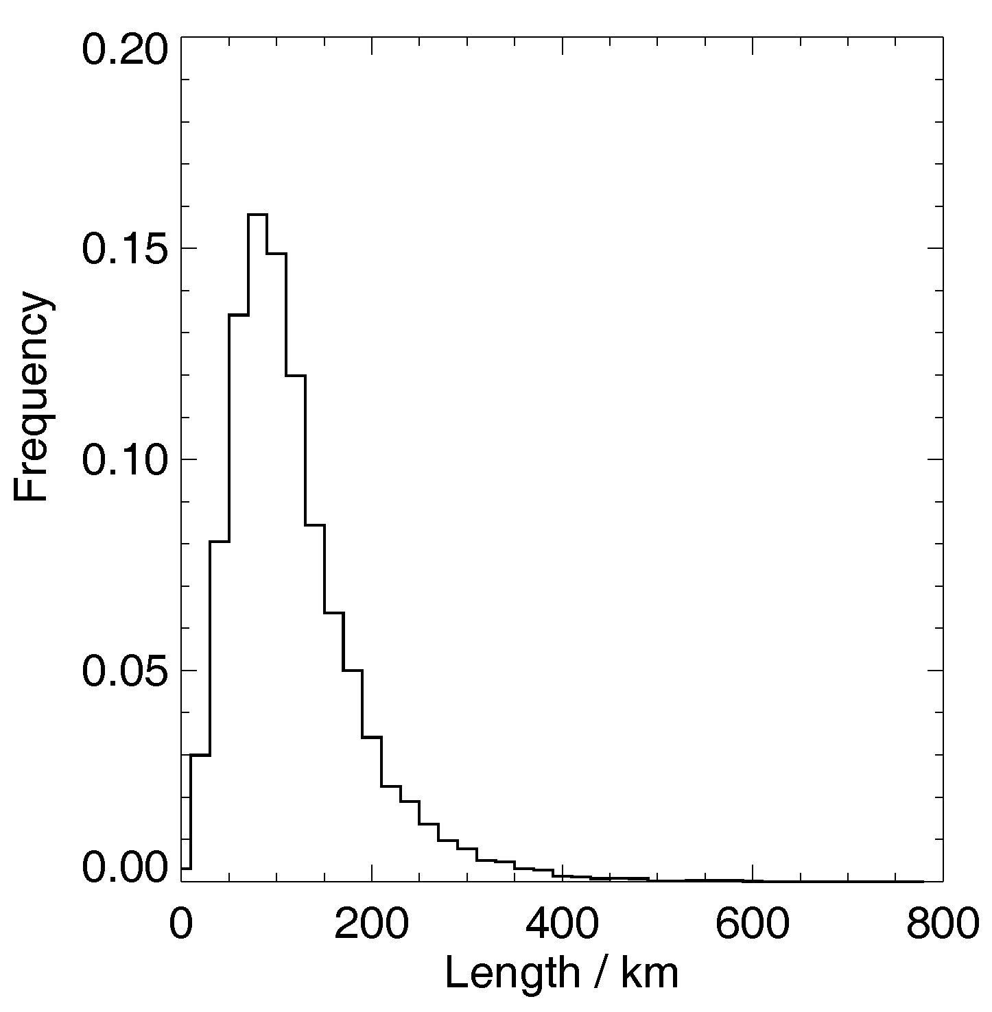
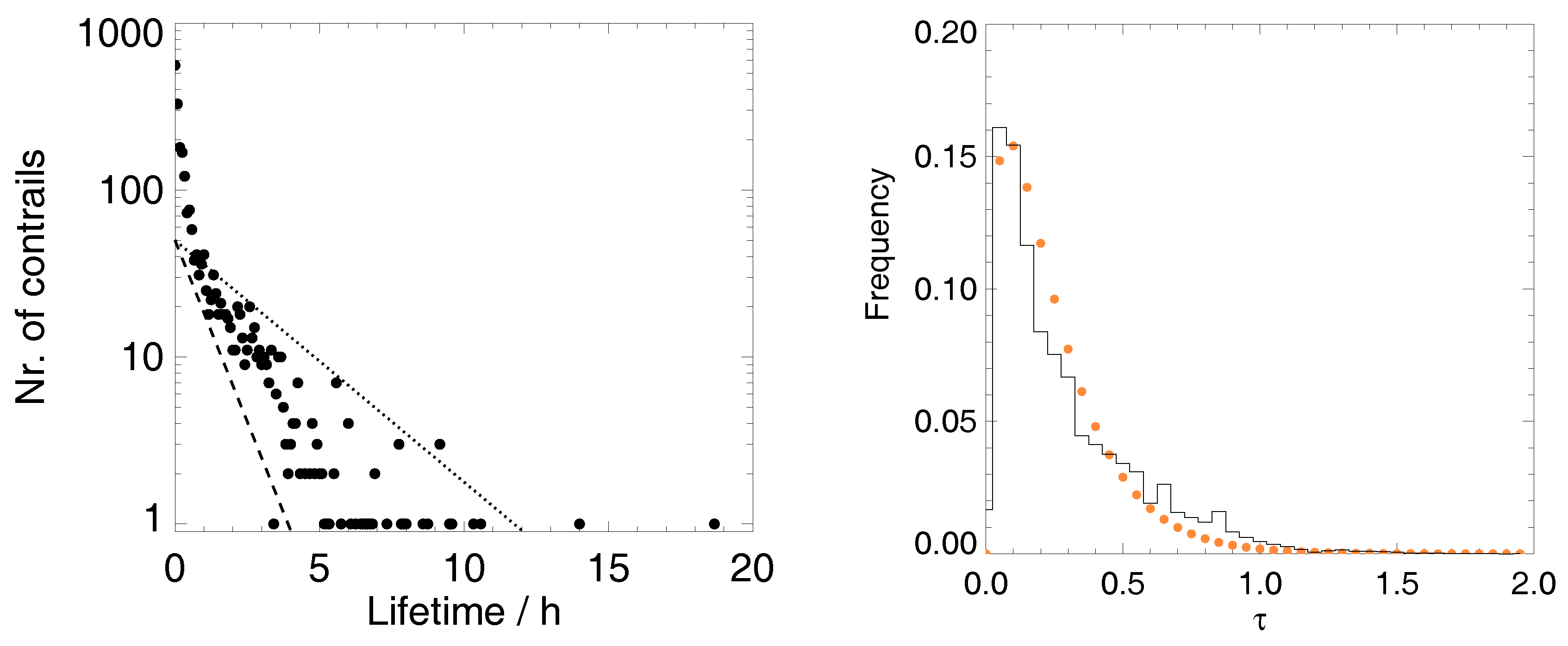
The particle size distribution largely affects the optical properties of contrails, which can be retrieved from satellite observations. Here we use the ACTA algorithm (for a complete description, please see [32]) described in Section 2.1.2. ACTA provides information on the dimension and lifetimes of the contrails (Figure 12 and Figure 13). Here, a mean effective length of 130 km is found, which is the distance between the two most distant ends of the contrail, even if they are not connected.
ACTA was combined with the COCS algorithm [93], which provides information about the optical depth and the cloud top height of cirrus clouds. A frequency distribution of the optical depth of the tracked contrails was derived (Figure 13, right). The dotted line represents the frequency distribution of a gamma distribution with shape parameter 1.5 and scale parameter 0.323. This is in good agreement with previous findings based on data from Cloud-Aerosol Lidar with Orthogonal Polarization (CALIOP) [94]. The average optical depth of our contrail set is 0.34. Our dataset had slightly shorter and optically thicker contrails than CALIOP. The geographic regions under consideration and the type of contrails were different. Studies of contrail outbreaks [95] show larger values of optical depth, consistent with our findings.
The combination of the ACTA results with a further algorithm, the Rapid Retrieval of Upwelling irradiances from MSG/SEVIRI (RRUMS), developed for the retrieval of top of atmosphere outgoing irradiance [96], provides insights on the strength of the RF of contrails. The RF is derived as the difference between the outgoing flux from the contrail pixels and that of a selection of the surrounding pixels [32]. The findings are presented in Table 1, separated for day and nighttime and for land and water surfaces, because we have used different criteria for the selection of the contrail-free pixels in those categories. Note that the sum of these four fractions is less than 100% as in 12% of the cases a clear land/sea or day/night identification was not possible. It can be seen that the largest contribution to warming is during night, where no shortwave forcing is present. During daytime the sum of the negative and the positive forcings provides a negative result, a net cooling effect [32]. These findings are in agreement with previous studies on contrail development [97,98,99].
The in-situ and remote measurements of contrails and contrail cirrus (shown above) provide important insights in their characteristics, whereas Large-Eddy-Simulations (LES) of contrails help to gain a deeper understanding of how contrails evolve and how they are affected by aircraft parameters and atmospheric conditions. The LES model Eulerian/Lagrangian numerical solver (EULAG) [100] together with the fully coupled Lagrangian ice microphysics scheme Lagrangian Cloud Model (LCM) [101,102] was employed for high resolution simulations (mesh sizes of 1 to 10 m) of young and aged contrails. For young contrails (age < 5 min) the interaction with the aircraft-induced downward moving wake vortices is the dominant feature. The analyses focus on how deep the contrails are after the vortex break-up and how many ice crystals are lost due to adiabatic heating. Both properties, the contrail geometric depth H and the total ice crystal number N, depend on many ambient and aircraft properties and are relevant for the late-time contrail-cirrus evolution [103]. To fully understand the complex processes, it is necessary to disentangle the effects of the various parameters. Unterstrasser et al. [104] deal with parameter variations that directly affect the wake vortex descent and break-up (thermal stratification, turbulence, initial vortex properties), whereas Unterstrasser [
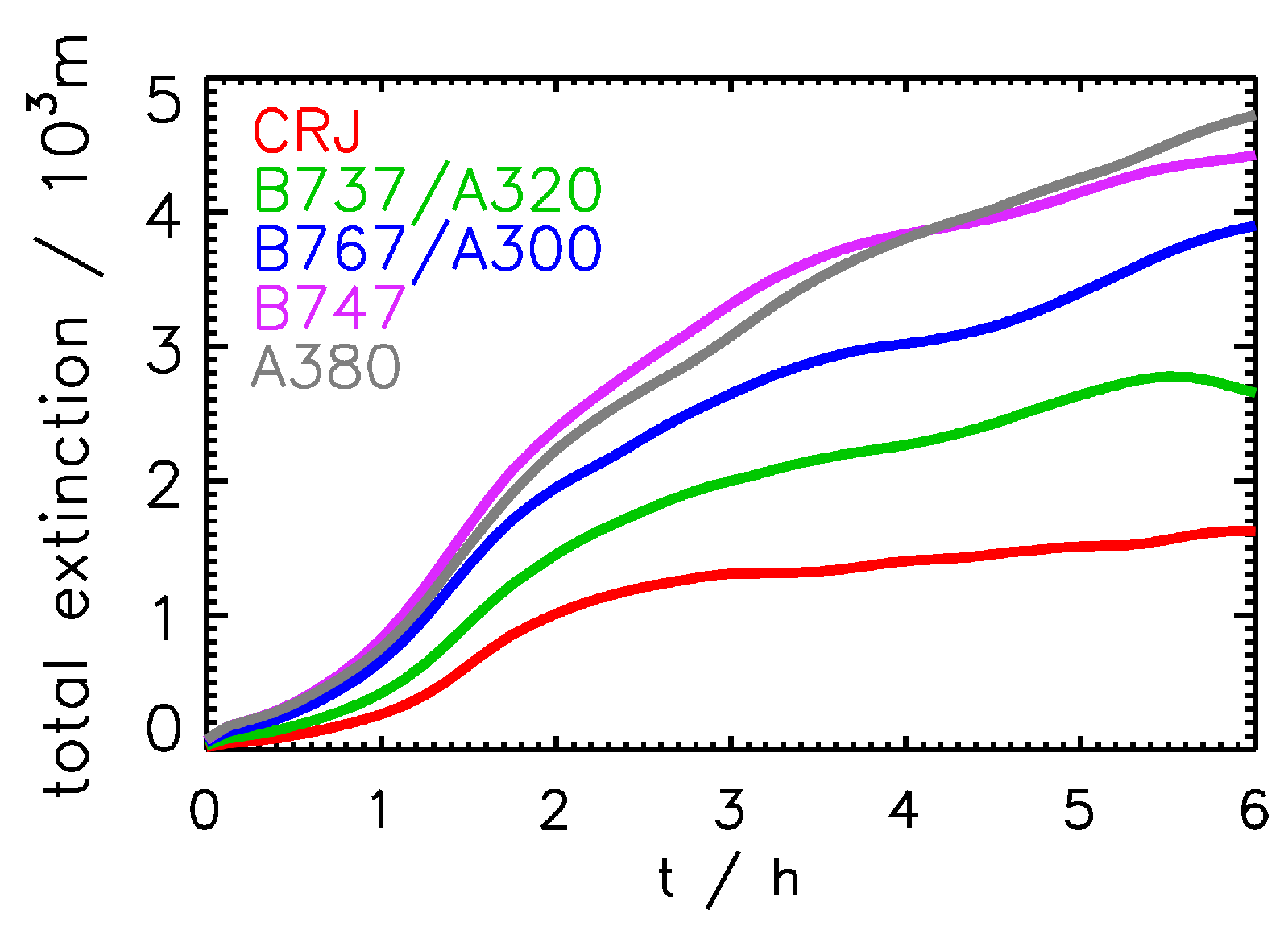
103] focuses on parameters directly relevant to contrail ice microphysics (temperature, relative humidity, soot emission index). In a next step, the importance of aircraft type on contrail evolution is assessed (ranging from a small regional airliner Bombardier CRJ to the largest aircraft A380 [105]). Differences in wake vortex properties and fuel flow affect the early contrail properties leaving a long-lasting mark over the simulated 6 hour period. For a selected atmospheric scenario, the total extinction (=product of mean optical depth and contrail width, see definition in [106]) is higher for larger aircraft (Figure 14). From the large dataset of LES presented in the three latter studies, analytical parametrizations of H and N taking into account the effects of temperature, relative humidity, thermal stratification and aircraft type (mass, wing span, fuel flow) could be derived [107]. The parametrizations are suited to be incorporated in larger-scale models where they can refine the current contrail initialization methods.
For aging contrails, sedimentation, radiative cooling/heating and atmospheric dispersion become relevant processes besides deposition/sublimation. Separate simulations of contrail-to-cirrus transition and of natural cirrus over up to ten hours were performed [
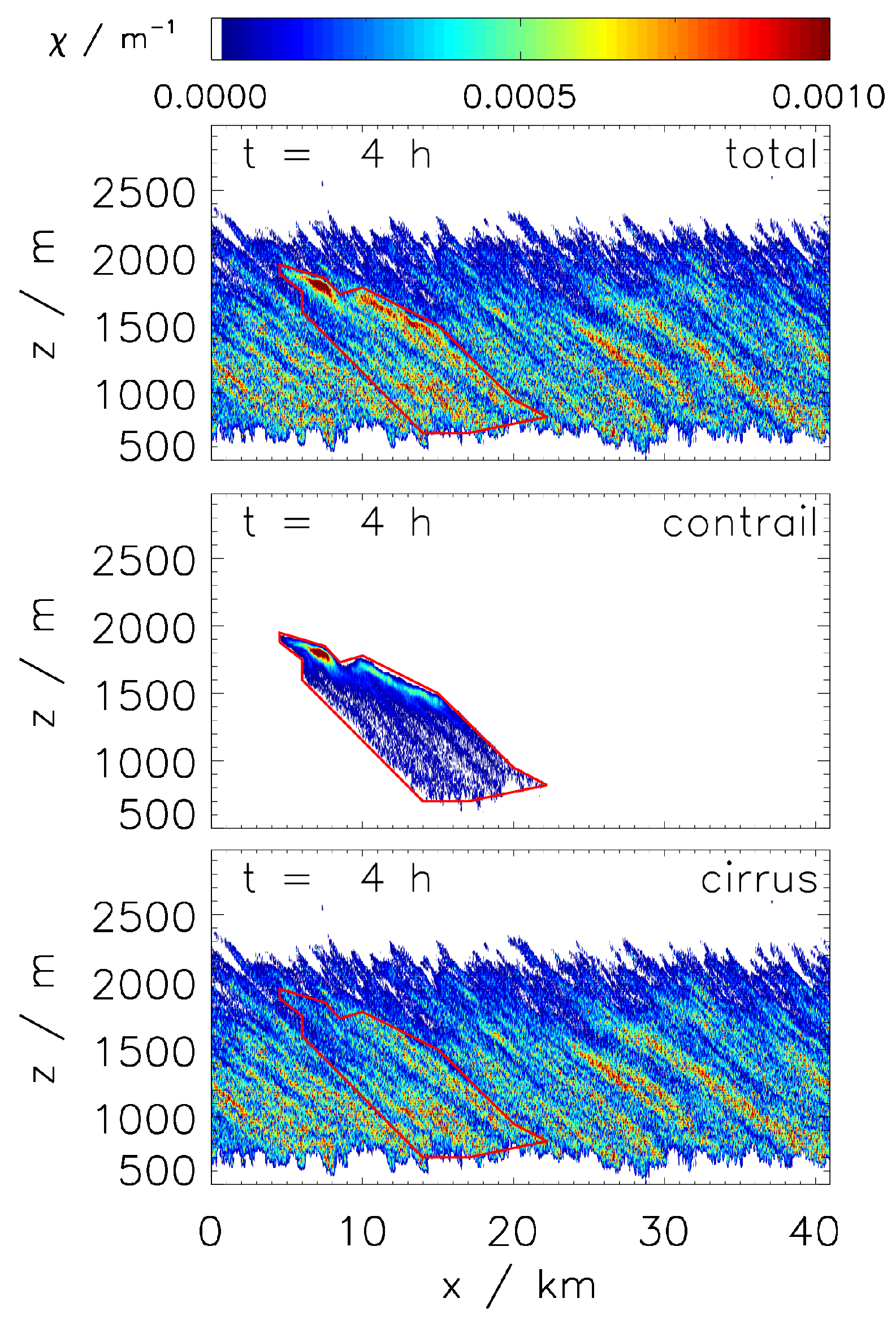
108]. It is found that weak but long-lasting updrafts allow for the longest life times of contrail-cirrus, whereas for natural cirrus, the updraft speed during their formation is most crucial. Contrails lose their linear shape over time and become hardly distinguishable from natural cirrus which makes it difficult to evaluate the extent and effect of the anthropogenic cloud modification. Even though the two cloud types have quite different formation mechanisms we could not single out microphysical criteria from the simulations that could help to distinguish in general between both cloud types in observations. In a next step, the interaction of contrail-cirrus and natural cirrus is analyzed [109], hereby focusing on the question whether a contrail remains identifiable as such, once it becomes surrounded by natural cirrus. The simulated extinction coefficient of such a scenery (top row in Figure 15) suggests that contrails embedded in cirrus do not generally remain identifiable in observations. The second and third row show the extinction of only the contrail or the natural cirrus ice crystals (the sum of both plots gives the top row). Cirrus ice crystals exist in large parts of the contrail (ice crystals in the bottom row are present inside the red polygon). In such cases the two cloud types are so intimately connected that it is no longer possible and moreover no longer meaningful to make a strict separation into a cirrus area and a contrail area.
Aircraft produce two kinds of condensation trails, exhaust contrails and aerodynamic contrails. The climate impact of exhaust contrails and the contrail cirrus resulting from them is a research topic since many years. In terms of RF it is estimated to be of the order 30–40 mW/m 2 with a quite large uncertainty [5,14,15,110,
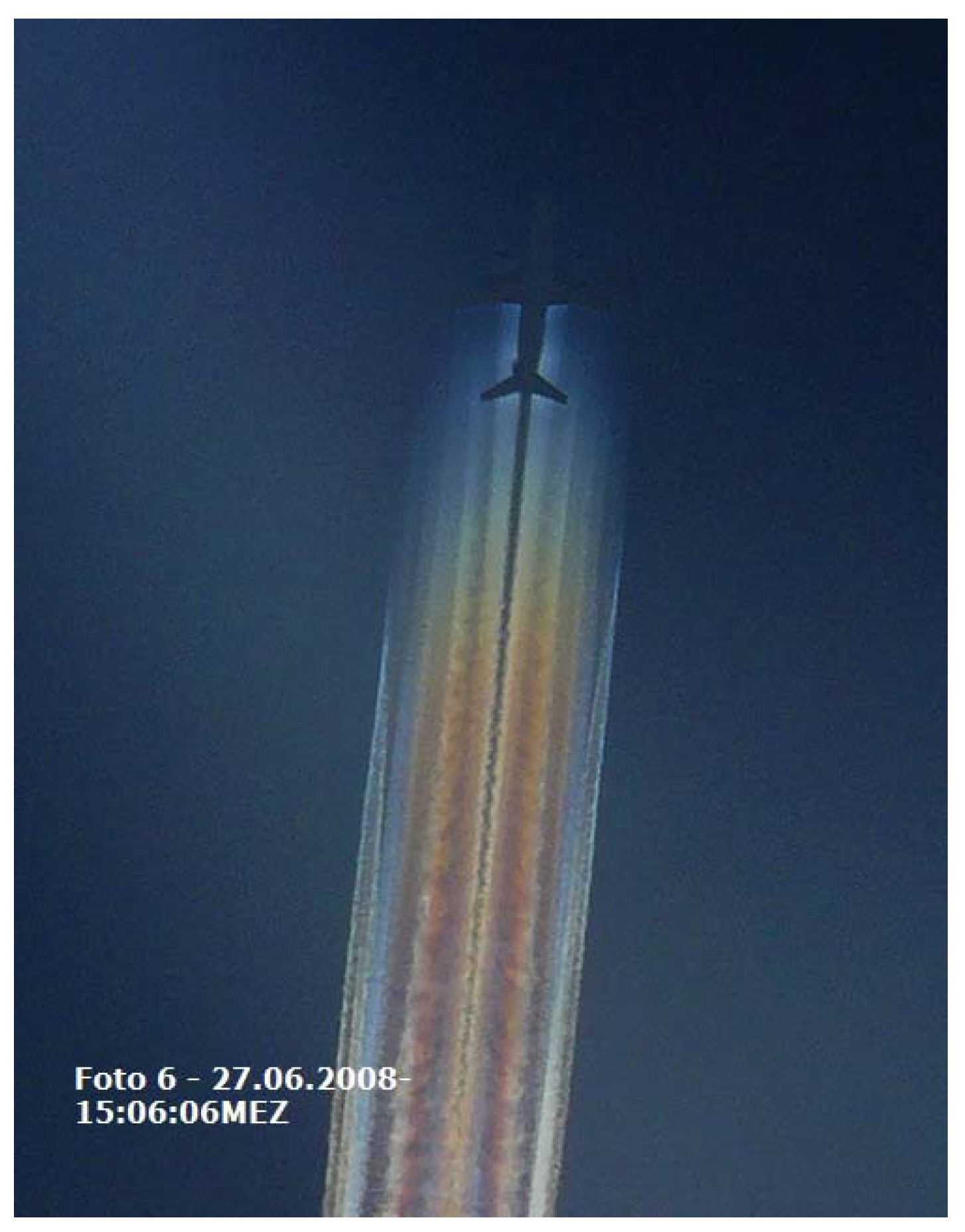
111]. The climate impact of aerodynamic contrails (Figure 16) is qualified to be very small compared to that of exhaust contrails [112], without providing a quantitative estimate of their RF. This qualification is based on the assumption that aerodynamic contrails form from freezing of liquid aerosol droplets in the airflow over the wings [113]. Jansen and Heymsfield [114] argue for another formation pathway, involving homogeneous droplet formation (HDN, i.e., formation of water droplets without the need for condensation nuclei), followed by homogeneous ice nucleation (HIN, freezing) on sufficient cooling of the droplets over the wing. A climatology of aerodynamic contrails using the thermodynamic conditions for HDN and HIN does not yet exist, neither an estimate of the corresponding RF. It is expected, yet, that the qualification of Gierens and Dilger [112] is still valid, namely that aerodynamic contrails have a much smaller climate impact than exhaust contrails.

3.2. Nitrogen Oxides and Reactive Species

Combining aircraft measurements with comprehensive climate-chemistry-modeling allows to study relevant atmospheric processes and to further investigate chemical impacts of aviation NO x emissions. During the HALO ML-CIRRUS mission in 2014 both measurements of contrails and reactive species were performed to characterize the probed air masses. Here we first compare modeling results with ML-CIRRUS observations to assess the model performance and then investigate the relation between atmospheric conditions and the aviation NO x impact on ozone. Ozone (O 3 ) was measured using the fast UV-absorption spectrometer FAIRO [116]; nitrogen oxide (NO) and the sum of all reactive nitrogen species (NO y ) were detected by the chemiluminescence detector AENEAS [83]. For the period of the ML-CIRRUS measurement campaign (March and April 2014, Section 2.1.1) a multi-scale (global/regional) hindcast simulation was performed with the MECO(1) model system, where ’1’ indicates one high resolution regional nest of the COSMO model in the global EMAC model (Section 2.2.1) and compared to observational data from ML-CIRRUS. 
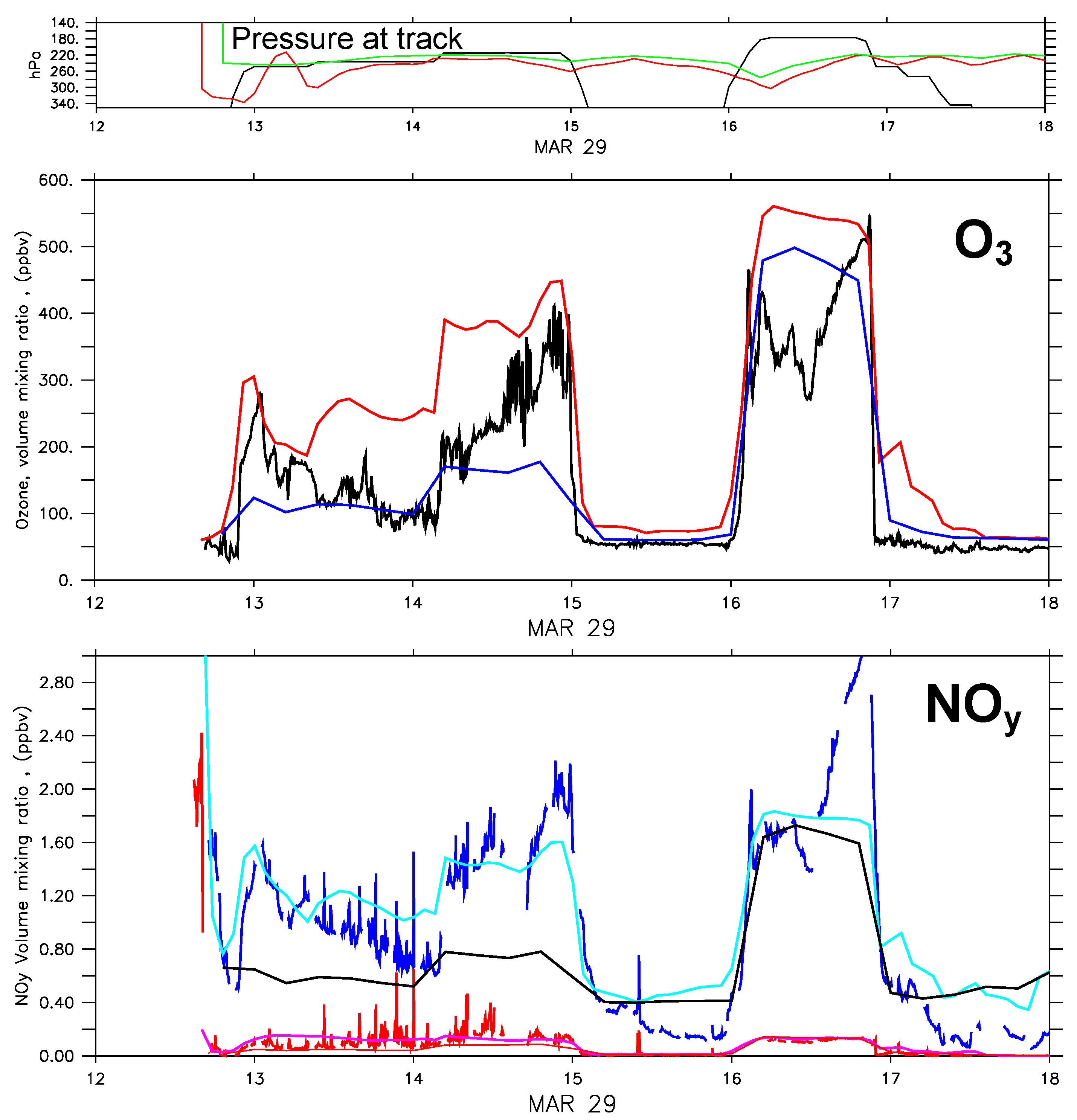
Figure 17 shows results of this comparison for the flight on 29 March 2014. After takeoff HALO turned northwards, then westwards and flew over France from north to south. At the southernmost point of the flight track over northern Spain, HALO turned to the northeast and finally headed for the Balearic Islands before returning to Oberpfaffenhofen. During the first part of this flight small scale enhancements in measured NO (lower panel; thick red line) and NO y (lower panel, blue line) in connection with high NO:NO y ratios (not shown) indicate the interception with several aircraft plumes in the tropopause region. Observed ozone values of up to 500 ppbv suggest that during three flight segments (middle panel; 13:00; 14:00–15:00; 16:00–17:00 UTC) stratospheric air masses have been encountered at altitudes between 11 and 12 km. Total reactive nitrogen with maximum values up to 3 ppbv are well correlated with high ozone values, especially in the lowermost stratosphere.
Simulated ozone mixing ratios along the HALO aircraft trajectory show similarly a quick increase to values of 100 nmol/mol and higher (EMAC; mid panel; blue line) and values above 200 nmol/mol in the COSMO instance (mid panel, red line), once the aircraft reaches a pressure altitude of 280 hPa according to on board measurements. While EMAC simulates lower ozone mixing ratios than observed during parts of the flight leg, COSMO shows a tendency to simulate higher ozone values. Taking a closer look at relative position versus the tropopause in the two models, a clear link becomes apparent. While aircraft altitude relative to the tropopause level in EMAC is very small (i.e., the aircraft is located near EMAC tropopause level), in COSMO aircraft altitude during large parts of the flight leg are located clearly above the tropopause, with pressure differences of up to 50 hPa, i.e., aircraft is clearly located in the COSMO stratosphere.
This means that the tropopause level in EMAC is simulated at higher altitudes, corresponding to a lower pressure of 200–220 hPa, compared to COSMO where the tropopause during parts of the flight is clearly diagnosed at lower altitudes, corresponding to a higher pressure level between 240 and 300 hPa, in some parts as high as 340 hPa. Consequently, EMAC values locate measurements close to the tropopause level, while COSMO attributes flight altitude already to the lower stratosphere, which explains lower ozone values in EMAC than in COSMO calculated along the HALO aircraft trajectory.
This behavior of different vertical positioning of the tropopause is persistent during the whole course of the flight, leading to lower values in EMAC (associated with lower tropopause pressures) compared to COSMO. An altitude change over Northern Spain is associated with an increase of ozone mixing ratios, in observations (120 nmol/mol increase) and both model simulations, in EMAC 50 nmol/mol and in COSMO 150 nmol/mol. During the flight leg, which is diagnosed by both models of being just above the tropopause (16:00–17:00 UTC), COSMO overestimates ozone concentrations between 20 and 150 nmol/mol, while EMAC initially agrees well and later underestimates ozone by about 100 nmol/mol.
In the EMAC simulation, NO y volume mixing ratios are underestimated compared to the observations by up to a factor of two, while COSMO reproduces variations of NO y values within 20%. NO values in COSMO are slightly higher than in EMAC. EMAC values and observations agree well within the uncertainty.
The results clearly indicate that the COSMO instance is better able to resolve regional-scale tropopause variations so that regional-scale measured ozone and especially NO and NO y enhancements can be better represented (13:00 and 15:00 UTC). Despite the horizontal and temporal resolution of around 250 km and 12 min of the global model (EMAC), EMAC is able to capture to some extent regional scale variations in the tropopause region, where large vertical gradients of the ozone, NO, and NO y mixing rations exists. The EMAC simulation agrees better with measured concentrations of NO, NO y , and O 3 in the period 15:30 UTC to 17:00 UTC than during the time before. The meteorological situation differs significantly in these two periods. A high pressure ridge is located in the area from the Balearic Islands to the Baltic Sea (not shown). The aircraft entered this area in this second time period, and hence the larger scale meteorological high pressure ridge is better represented by EMAC than smaller scale atmospheric perturbances during the first part of the flight leg, which was west of the high pressure ridge.
It is well established that the magnitude of the contribution of aviation NO x emissions to the ozone concentration depends on the location of the emissions in terms of altitude [49,117], geographic region [118], but also time of the year [119].
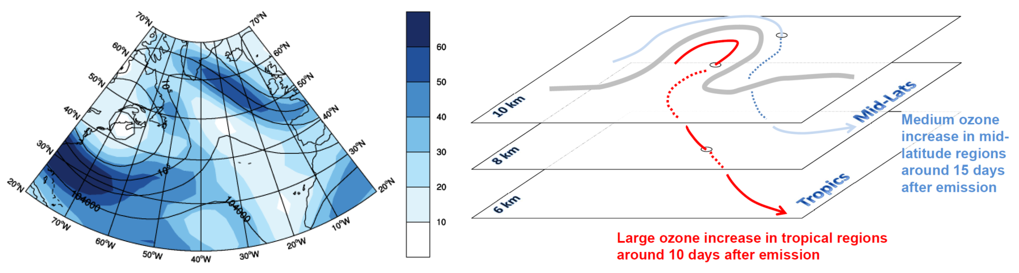
Here, we investigate to what extent the location within a weather situation affects the ozone production [81]. 
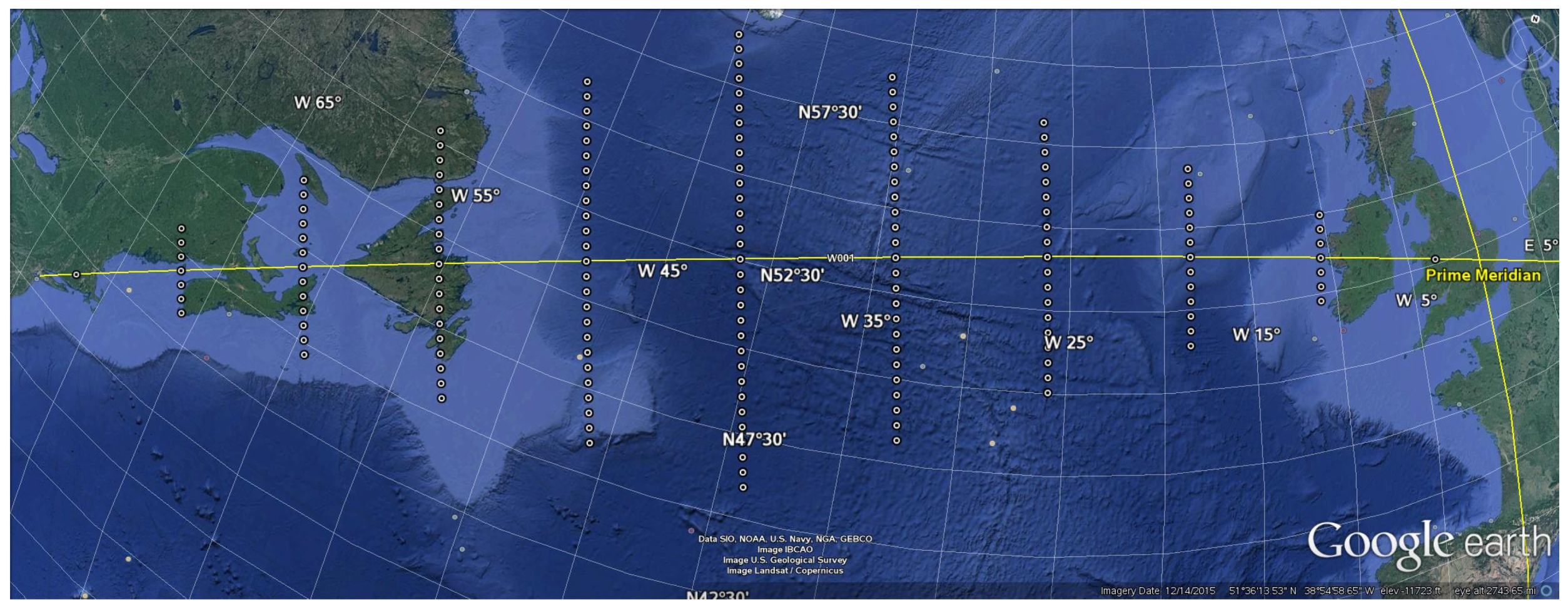
Figure 18 shows the investigated weather situation (left), with a high pressure ridge (HPR) reaching from western Africa to the tip of Greenland (low geopotential height) and hence even larger than the high pressure ridge discussed above. We have investigated 150 air parcel trajectories starting in the area of the HPR (40 ° N to 50 ° N at 15 ° W) and west of it (40 ° N to 50 ° N at 30 ° W) for this weather situation and did the same for a similar blocking situation. The results clearly show a distinct difference of the transport pathway and the chemistry along the trajectories starting inside and west of the high pressure ridge, which is summarized in Figure 18 (right). The trajectories starting within the HPR are transported to lower altitudes and show a contribution from aviation NO x emissions to ozone at lower altitudes, more southward, and earlier (Table 2). The trajectories starting inside the HPR show an adjusted RF and CCF from the ozone change, which is roughly 50% larger than that of the trajectories starting west of the HPR (Table 2). This is basically a result of the more intense ozone chemistry at lower latitudes, which leads to larger contributions of aviation NO x to ozone for emissions in the HPR.

3.3. Aerosol Effects

Aviation-induced effects on aerosol concentrations and resulting climate impacts were investigated using the EMAC model coupled to the aerosol submodel MADE. The adopted model configuration takes into account the interactions of aerosol with clouds and radiation (see [17], for more details). The effects of aviation are estimated by comparing two simulations, one with and one without aviation emissions (the so-called 100%-perturbation method [120,121]). The simulations were performed driving the model with meteorological analysis data for temperature, surface pressure and winds over a 10-year time period (1996–2005). This allows to reduce the noise arising from different meteorological conditions when comparing two free-runing climate simulations [122].
Emissions of short-lived gases (NO x , CO, SO 2 , Non-Methane Volatile Organic Carbons (NMVOC), and NH 3 ) and aerosol species (black (BC) and organic carbon (OC)) from the Coupled Model Intercomparison Project Phase 5 (CMIP5) inventory [123] were used as input to the model. This inventory was specifically developed for the multi-model studies conducted in support of the 5th Assessment Report of the Intergovernmental Panel on Climate Change (IPCC). It provides historical emissions up to the year 2000 and future projections based on Representative Concentration Pathways (RCPs [124]) up to the year 2100. In this study, we therefore chose the year 2000 as baseline estimate and a relatively close time horizon (year 2030) to analyze future impacts. This was done in order to limit the uncertainty from the scenario projection, which is usually growing with the projection time [125]. Since the CMIP5 emission inventories do not include aviation sulfur emissions, these were estimated from the aviation BC emissions based on the respective emission factors of the two species. Aerosol number emissions were calculated under various assumptions on the size distribution of the aircraft-emitted particles. Additionally, a scenario for low-sulfur aviation fuel was considered for the year 2000 only [17].
The model results show a distinct impact of aviation on aerosol concentrations in the northern mid-latitudes, at the typical flight altitudes between 400 and 200 hPa. Significant effects were also simulated for the ground level and are related to emissions from airport activities and landing and take-off LTO cycles, and to downward transport, especially in the subtropical jet region. The year 2000 impact on aerosol particle mass (black carbon and sulfate) is of the order of a few ng/m 3 (corresponding to a few percent in relative terms), whereas aviation-induced increases of the order of 1000 particles/cm 3 (30%–40%) were simulated for aerosol number concentrations, as a result of sulfur emissions. These impacts were projected to grow in the future, with aviation-induced mass and number concentrations increasing from 2000 to 2030 in all scenarios, in particular in RCP2.6. It is however important to mention that the RCPs do not consider any technological change in the fleet for the future, as it is done in more aviation-specific emission scenarios, but rather project a steady increase as a direct consequence of the increasing air traffic volumes.
Such aviation-induced changes in aerosol concentrations also lead to climate-relevant effects. Aerosol particles can affect the planetary radiation budget both directly, by scattering and absorbing radiation, and indirectly, by perturbing the microphysical structure of clouds, thereby changing their albedo and lifetime [126]. Note that the model setup adopted here only considers aerosol interactions with low-level, liquid clouds. Aerosol-induced formation processes of ice particles (
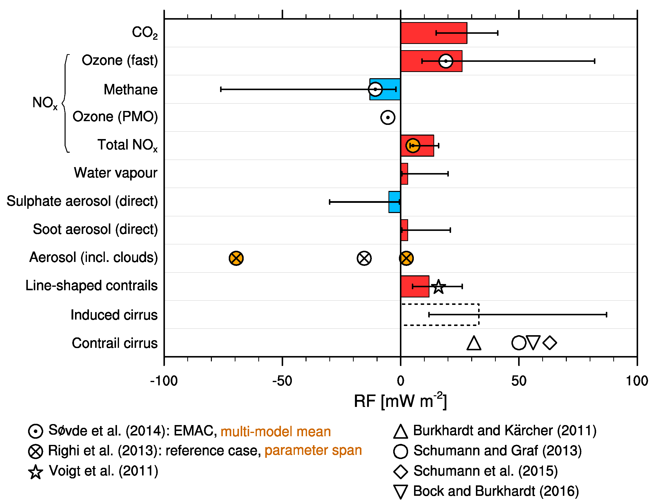
Section 2.2.2) were not yet taken into account. According to our numerical experiments, aviation-induced aerosol is responsible for a RF ranging between –69.5 and +2.4 mW·m 2 in the year 2000, depending mainly on the assumed size distribution of emitted particles and on the assumed sulfur content of aviation fuel (Figure 19). Hence, this cooling effect could potentially be larger than the warming effect induced by other aircraft-induced compounds, such as CO 2 , ozone, and the effect of contrail cirrus. An in-depth analysis of the radiation perturbations in the model indicates that the bulk of the aerosol RF is ascribable to the aerosol-cloud interactions. Further analyses, including also a sensitivity experiment with low-sulfur aviation emissions, also suggest that aviation-induced aerosol sulfate is the key component in this context, being transported downward from the flight levels to relatively low altitudes where it affects cloud droplet number concentration and radius. Hence perturbations to low-clouds are driving the large RF simulated here, as also reported in similar studies [21,127]. In agreement with these investigations, our analyses also reveal that the assumptions on the size distribution of emitted sulfur particles are essential. The large negative forcing described above is only simulated if an emission of large numbers of ultrafine sulfate particles is assumed. These results further suggest that BC plays a minor role in affecting warm clouds, due to its small contribution to total aerosol number and mass concentration. Recall that possible BC effects on cirrus are neglected here. Also aerosol nitrate plays a minor role in this context. We assume that the emitted mass of ultrafine particles, which are essential for the modelled cooling effect, is controlled by sulfate [128]. Hence the aerosol-induced cloud modifications are driven by sulfate rather than nitrate. In addition, aerosol nitrate is found to decrease as a consequence of high aviation sulfur emissions and the sulfate-nitrate competition for available ammonia in the upper troposphere. Note that aircraft-induced aerosol nitrate and sulfate can also have significant cooling effects due to direct interactions with radiation. This cooling is however compensated by the warming effect of aircraft-generated BC (see e.g., [129]), which explains the minor role of direct aerosol-radiation interactions in our simulations. Given the aforementioned growth in traffic volumes, the simulations with the RCP scenarios result in a factor of 2 to 4 higher (more negative) RF in 2030, albeit with large uncertainties related to the assumptions on the size distribution of emitted particles and on the fuel-sulfur content of aviation fuel, which might experience large changes in the near future.
The large aerosol effects found by this model study opens additional perspectives for future mitigation strategies and climate policies. Aerosol-cloud interactions will have to be considered in future assessments of mitigation options, which we have not yet included in our studies (Section 4.1, Section 4.2, Section 4.3, Section 4.4 and Section 4.5). This is relevant in particular in view of desulfurization of jet fuels which is already being considered in the aviation sector [130]. Another aspect, which has not been considered in this analysis, is the impact of aviation on cirrus clouds. As discussed in Section 2.2.2, the model was extended to also account for aerosol interactions with ice clouds. It is now technically possible to simulate such effects in EMAC, but uncertainties are still large and more in-depth research, including also detailed measurements from in-situ and laboratory experiments, is required in order to achieve a more robust model representation of ice formation processes in the upper troposphere.

3.4. Climate Metrics

The assessment of mitigation options requires a good understanding of the underlying physical and chemical processes, from the emissions to RF (see previous chapters), and an adequate aggregation of these effects. Climate metrics are frequently used for aggregation, putting the different effects on the same scale. This is a non-trivial exercise, since the lifetime of the individual effects have different orders of magnitude. Contrails exist for hours, whereas emitted carbon dioxide change the atmospheric carbon dioxide concentration for centuries. What is more important, a small RF caused by a carbon dioxide concentration change, but prevailing for centuries, or a large perturbation in radiation due to contrails, which, however, exists for a short period, only? It has often been stressed in literature that results, obviously, depend on the choice of the climate metric, which is a political rather than a scientific choice [131]. As a result, climate metrics, or the choice of climate metrics were perceived as equivocal. Grewe and Dahlmann [132] pointed out that the different climate metrics, although targeting somehow climate change, are providing “different physical quantities measuring climate change and hence they provide answers to different questions”. Therefore it is important to first address, in a detailed manner, the overall climate target. This could be “Is a given technical (or operational) measure suited to contribute to the 2 ° C target (in comparison to conventional approaches)?”. This is already the first of the five steps proposed by [132] for choosing an adequate metric, answering the posed question:
  • Precisely posing the respective question,
  • Deducing from the question an adequate reference,
  • Deducing from the question an adequate emission scenario,
  • Deducing from the question an adequate climate change indicator/ metric,
  • Deducing from the question an adequate time horizon.
In the given example Steps 2–4 could be a “business as usual (conventional technology)” as a reference, a future emission scenario, which includes the respective measure, temperature change, and a time horizon related to the time horizon of the 2 ° C target, e.g., a mean over 100 years after introduction of the measure. Obviously, other combinations, such as a pulse emission and global warming potential are not suitable to answer this question. Having agreed on the question leads to only few possibilities in the choices of Steps 2–5. This subset of suitable metrics gives quite similar answers to the question posed, as first results indicate [7]. That is, the answer and subsequent decisions based on it are no longer equivocal.

4. Measures to Reduce the Climate Impact of Aviation

4.1. Strategic Technological Measure: Strut-Braced Wing Aircraft Insertion

We combined the capabilities of modeling the atmosphere (Section 2.2) and air traffic system modeling capabilities (Section 2.3) to investigate the effectiveness of both technological and operational measures to reduce the climate impact of aviation. Among the strategic mitigation options we have chosen a Strut-Braced Wing (SBW) aircraft equipped with a counter-rotating open rotor (CROR) engine as a technical measure and the concept of Intermediate Stop Operations (ISO) as an operational measure.
SBW aircraft that are characterized by supporting struts linking wings and fuselage are mainly known from General Aviation (e.g., Cessna 172) as they provide several advantages. Such a wing construction eventually leads to a higher aerodynamic efficiency due to an increased aspect ratio and reduced weight compared to conventional cantilever wing aircraft of the same size. As a consequence also smaller engines might be used that in turn reduce fuel consumption and produce less emissions [133]. Hence, researchers and engineers are currently investigating how such a SBW configuration could also be realized on commercial aircraft. We analyzed to what extent such a new SBW aircraft design could be beneficial for the climate impact of aviation by applying the four-layer approach described in Section 2.3.1. The aircraft model (geometry, weights, aerodynamic and engine performance) was provided by the DLR-internal project on Future Enhanced Aircraft Configurations (FrEACs). Figure 20 shows the geometry of the designed aircraft and Table 3 lists the main design characteristics.
As appropriate engine a so-called CROR was selected, which allows for a significant reduction of NO x emissions due to a special two-stage lean combustion technique [134]. For the study, it was assumed that the SBW serves as a substitute for the next generation of aircraft with 101–150 seats (e.g., Airbus A320, Boeing 737 successors) and that the introduction of this new generation (N+1) starts in 2015. Using a fleet renewal model the share of SBW aircraft in service was estimated as a function of time until 2050 (see [59] for more information). Then, from the worldwide flight schedule (see previous section) and the corresponding air traffic forecast from AIRCAST (see Section 2.3.1) all flights of that seat category were filtered and—using GRIDLAB—these flights were simulated with an Airbus A320 aircraft model as a reference to obtain the fuel and emission distribution for the business-as-usual scenario (current aircraft technology level maintained until 2050) for all years. In a next step, the same flights were simulated with the SBW aircraft performance model to generate the SBW inventories. Afterwards, both A320 and SBW inventories were mixed using the weighting factors from the fleet renewal model. Figure 21 shows the effects of SBW operations in 2050 on the global fuel consumption.
According to that, by 2050 the share of SBW reaches 93% of all aircraft in the 101–150 seats category. By that time, the introduction of SBW may lead to 26% less fuel and even nearly 45% less NO x emissions. The climate impact assessment was performed with the chemistry-climate response model AirClim with the objective to estimate the changes in the long-term climate impact from aviation by introducing a fleet of SBW aircraft in comparison to conventional technologies (see Section 2.2.3 for more details on climatological CCFs). A future emission scenario (IPCC-FA1), conventional technology as a reference and the global mean near-surface temperature change over 100 years (ATR 100 ) after introduction of the SBW fleet is an adequate metric to assess the climate impact of this technology (see Section 3.4). Note that a background atmosphere with inceases in CO 2 and CH 4 concentrations is taken into account. We found that the projected warming (in terms of ATR 100 ) caused by global air traffic of that category may be reduced by approximately 17% due to SBW operations (see Table 4 for the agents’ individual contributions).
This reduction in the climate impact of aviation in comparison to a conventional technology can be mainly attributed to the significantly lower NO x emission at cruise altitude together with a slightly reduced average cruising altitude, as the optimum altitude of the designed SBW aircraft is lower than the one of a conventional A320. Note that changes in particulate emissions, such as soot, were not taken into account. A reduction in the soot number densities from lean combustion would result in changes of the properties of the contrails (lower ice particle densities, lower shortwave optical thickness, and enhanced sedimentation of ice particles), which would lead to a much larger decrease of the climate impact by contrails [136,137,138]. A detailed description of the study can be found in [135].

4.2. Strategic Operational Measure: Intermediate Stop Operations

Previous research has demonstrated that executing intermediate landings for refueling aircraft at suitable stopover locations during long-haul flights can significantly reduce fuel burn and partially lead to a decrease in airlines’ cash operating costs as well [139,140,141,142,143,144,145]. This technique is called Intermediate Stop Operations (ISO) and also known as Staging service. Based on these findings, one would usually expect a climate impact reduction if ISO was adopted on a global scale. However, as the actual climate impact of such a change in the way the aircraft is operated is not only dependent on the amount of emissions—which predominantly is reduced by ISO due to the enhanced fuel efficiency—but also on the redistribution of the emissions both geographically and altitudinally, a systematic approach is required that models the implementation of the concept under real-world conditions.
In the same manner as for the climate impact assessment of a SBW fleet in Section 4.1, we used the four-layer approach described in Section 2.3.1. The system-wide study was carried out assuming that existing aircraft types are used (current fleet), so the same aircraft type is used for the ISO mission as the one that is operating the direct flight. Based on a worldwide flight schedule from 2010, first all flights relevant for ISO (these were found to be all wide-body aircraft-served missions longer than 2500 NM) were identified. For the business-as-usual scenario those flights then were simulated using the trajectory layer functionality realized by the modeling system GRIDLAB in order to obtain fuel consumption values and engine emission inventories resulting from direct flight operations. In a next step, for each of these missions a set of adequate stopover locations was defined and among those airports the optimum one—leading to maximum fuel savings—was identified using exhaustive search. Then again, missions were simulated—this time assuming an intermediate stop at that optimum airport. Due to the split in two flight segments, aircraft does require less fuel and thus is significantly lighter at take-off on ISO missions. This in turn results in higher average cruise altitudes as the optimum altitude which the pilot tries to acquire increases with decreasing aircraft mass. This phenomenon leads to a significant shift of cruise emissions to higher altitudes (by approx. 4000–6000 ft), which was observable after generating the ISO mission emission inventories by GRIDLAB. Figure 22 shows exemplarily the fuel consumption changes caused by ISO as a function of geographic location and altitude.
The inventories show that if ISO was adopted globally, this could reduce the global wide-body aircraft fuel consumption by 4.8% and for about 87% of those flights at least one airport can be found that leads to fuel savings if used as stopover location. Also CO 2 , H 2 O and SO 2 emissions can be decreased by 4.8% (they are produced nearly proportionally to the amount of fuel burnt). NO x emissions reduce by 4.6%. CO emissions increase by 33.3% and HC emissions by 43.4%, which is because these are primarily released in flight phases with low engine thrust level (e.g., during descent, approach, landing), which double due to ISO and may have a significant impact on local air quality.
Both business-as-usual and ISO inventories then were passed on to the chemistry-climate response model AirClim ([48,49] for more information) in order to estimate the changes in the climate impact. For that, as appropriate metric the Average Temperature Response over a period of 100 years (ATR 100 ) was selected. By that it is ensured that the effects of a continuous emission redistribution starting from the global introduction of the ISO concept (assumed 2015) and the dynamics in the climate system including concentration changes of RF agents are fully captured. It turned out that in spite of a reduction of some of the emission species there would be an estimated temperature increase (ATR 100 ) of about 2.3% compared to the business-as-usual scenario (all flights operated as direct flights).
This increase is composed of increased warming effects from NO x emissions (+2.12%) and H 2 O emissions (+1.26%) due to the higher altitude in which they are released (see also Figure 23). The reduced warming due to CO 2 (−0.72%) and contrails (−0.35%) cannot compensate this (see [61,146], for more details). Note that here we analyzed ISO on the basis of current technology and fuel optimal routings. A change in these overall assumptions, such as redesign of the aircraft, introduction of medium-range aircraft, economical feedback, climate-optimized routings, may have a significant effect on the results.

4.3. Tactical Operational Measures: Eco-Efficient Flight Procedures

Due to the strong dependency of non-CO 2 -emission’s climate impact on locus and time of emission, climate-optimized trajectories are considered as potential measure in order to reduce aviation induced climate impact [7,24,147,148,149]. However, avoiding regions, characterized by high specific climate impact with regard to aircraft emissions, is related to raising costs caused by detours and off-design altitudes [150]. Consequently, we focus on the trade-off between climate impact reduction and increased cash operating costs.
As a use case, climate optimized trajectories for several routes within the North Atlantic region were investigated in order to compare the potentials of 2D (lateral) and 3D (lateral and vertical) trajectory optimization [66]. Therefore, models for the cash operating costs (COC) as well as CCFs (see Section 2.2.3) were integrated into the objective function J of the Trajectory Optimization Module (see Section 2.3.2) according to Equations (8) and (9). COC are calculated as a function of mission time and mission fuel. The climate impact, measured as average temperature response (ATR, see Section 3.4), was estimated by integrating the product of CCF and emission flow m ˙ i of species i (or true air speed v TAS for contrail induced cirrus clouds, CiC) along the trajectory. In order to identify Pareto-optimal solutions, the climate weighting factor c Ψ was varied between 0 (minimum costs) and 1 (minimum climate impact).
J = c Y · C O C t mission , m fuel , mission · C O C r e f 1 normalized COC + c Ψ · i t 0 t f C C F i x , t · m ˙ i t d t + t 0 t f C C F C i C x , t · v T A S ( t ) d t · A T R 20 , t o t , r e f 1 normalized climate impact
with i C O 2 , H 2 O , N O x c Y + c Ψ = 1 with c Y , c Ψ 0 , 1
From the environmental point of view, the acceptance of deviations from the cost-optimal trajectory is beneficial, as long as the reduction of the specific climate impact predominates additional fuel burn and emissions resulting from lateral detours, additional climb and descent phases, headwinds as well as off-design altitudes (see Figure 24). The analysis of the North Atlantic region has shown that the climate impact mitigation efficiency (ATR reduction per COC increment) is much higher if vertical trajectory changes are permitted. For example, by allowing the COC to increase by 2 %, climate impact can either be reduced by 15 % with 2D-optimization or by 45 % with 3D-optimization. Additionally, a maximum climate impact mitigation potential of about 20 % for laterally (2D) optimized trajectories and almost 60 % for laterally and vertically (3D) optimized trajectories is observed (see Figure 25). However, in both cases, the climate impact mitigation efficiency decreases rapidly for high COC margins. Hence, a reasonable and eco-efficient trade-off between the accepted cost increase and the climate impact reduction needs to be elaborated. Grewe et al. [7,151] optimized aircraft trajectories including lateral and altitude variations, though latter was assumed to be variable but constant for a whole aircraft trajectory. Hence those results fall, by definition, in between the 3D- and 2D-optimization, shown here. In contrast, Schumann et al. [24] applied altitude changes for regions were persistent contrails can form. Their results show very large reduction potentials, indicating that the Pareto Front is, by definition, to the right of the line of the 3D-optimization, but probably close to it.
Avoiding climate sensitive areas implies changes in the traffic densities of individual air traffic sectors. Here, we are investigating how these shifts of the trans-Atlantic air traffic [7] affect the capacity of the entry and exit sectors, which connect the European airspace with the North Atlantic Track System (NATS). We are analyzing a whole traffic scenario, including the trans-Atlantic and European flights in a two step procedure. First simulating trajectories with TrafficSim (Section 2.3.2) for a base case and a climate optimal scenario, based on the REACT4C CCFs (Section 2.2.3, [7,81]). Second, we are analyzing the capacity with a commercial state-of-the-art fast-time simulation software (AirTOp) [152] taking into account a detailed representation of the European airspace. The evaluation methodology focuses on parameters such as number of flights, sector capacities, controller workload and number of affected flights with both horizontal or vertical change, and flight duration [153]. There are several fast-time simulations performed, which will analyze the feasibility of the climate optimized trajectories as well as the impact they have on the ATM system [152].
Figure 26 (left) shows the hourly demands of North Atlantic Flight Information Regions (FIR) for both the reference (top) and optimized scenario (bottom) covering 24 h. The highest demand in both scenarios can be found in the GANDER FIR. The peak hours for all the FIRs remain similar to the reference scenario, except for the slight change within the peak hours in the Reykjavik FIR.
Figure 26 (right) shows demands of those airspaces, which serve as entry points to the European airspace. Generally, differences between the reference and the optimized scenarios can be observed, but they are in the order of day-to-day variations. The BIRDSS airspace shows an increase in the number of peak hours (between 10:00 and 12:00), which temporarily might have an effect on the controller workload. Although the routing changes have only little impact on the number of flights in the FIR and entry point sectors per 1 h, the related flown distance shows more changes, e.g., in the BIRDSS airspace at 11:00–12:00 where it increases from 5000 NM to 6000 NM (not shown).
Figure 27 shows the controller work duration for each of the airspaces selected. The biggest difference can be noticed, as expected, in the work duration in the BIRDSS airspace, where the work duration increases for more than 10 min. But, on the other hand, we can see that some of the neighboring airspaces are relieved and the work duration in the EGTT09LND airspace lowers compared to the reference scenario.
Hence, the routing changes of the optimized traffic scenario do not significantly change the general traffic flow and implications on the airspace demand and controller workload are minor. Here, we have only investigated on specific day and hence, to receive a better understanding of the impact of the optimized traffic on the ATM operations in the European airspace, a more detailed analysis of the airspace structure and operations is necessary. Still, this result indicates that controller workload may not be a limiting factor for trans-Atlantic air traffic.

4.4. Implementation of Eco-Efficient Procedures

Climate-optimized procedures come along with an increase of cash operating costs (COC; see Section 4.3), but airlines have little incentives to bear these additional costs voluntarily. In environmental economic terms they can take the position of a free rider: even though, if they are not willing to share the costs of climate protection, they benefit of its non-excludability (=everyone may contribute to climate change) and non-rivalry character (=contribution to climate change is not limited). The crucial question is then, how to create a monetary incentive for airlines to minimize flight time and emissions in highly climate sensitive regions.
One environmental policy option is to impose a climate charge or a climate restriction for operators of aircraft which fly in these areas (Figure 28) [50,154]. In these concepts, an airspace area j is levied with an environmental unit charge U c j per kilometer flown d j , if its specific climate impact with respect to aircraft emissions exceeds a specific threshold value ( c thr ):
CCA j x = U c j , if CCF tot x c thr 0 , if CCF tot x < c thr
with x a location within the area j and U c j (total restriction) as an extreme case. Climate charges, C c j , are expressed for a flight through a climate charged area j in analogy to en-route and terminal charges:
C c j = U c j · MTOW k 1 k 2 · I a c · d j
where MTOW is the maximum take-off weight of an aircraft, I a c an incentive factor for climate-friendly technologies and k 1 , k 2 country-specific parameters [154]. Note that in this case the CCFs are aircraft specific (Section 2.2.3) and depend on Mach number and cruise altitude and thereby can be easily converted into climate impact per flown distance.
In order to cut climate charges and hence resulting COC, cost-minimizing airlines will choose to fly longer and re-route their flights away from more expensive airspace areas (trajectory 3 in Figure 28b,c). In this way, the cutting of costs coincides with climate impact mitigation. Alternatively, the operator of an aircraft can also minimize flight time and pay compensation for higher climate damage (trajectory 1 in Figure 28c). By extending the existing charge system of air traffic control with an additional climate charge, adjustment efforts for airlines are minimized: no handling of complex climate-change functions is required within the airline planning processes to reduce non-CO 2 climate effects (see also Section 2.2.3).
The climate impact mitigation efficiency of the CRA (Climate-Restricted Airspace) concept is shown in Figure 29, It is nearly as large as the corresponding efficiency of COT (Climate-Optimized Trajectory), that is, it is close to the optimum possible. CCAs are expected to be similarly promising while offering the benefit of being more operationally feasible.
Besides restricting areas or charging areas, market-based measures (MBM) are instruments to steer air traffic into the direction of a reduction of its climate impact. For 5 representative winter days and 3 representative summer days, which were selected according to Irvine’s classification [156], we have calculated CCFs, i.e., the impact of a unit aviation emission on climate (Section 2.2.3, [7,26,151]). Then a representative air traffic scenario (roughly 800 flights) was taken into account to optimize each trajectory with respect to costs (fuel and crew) and climate impact and an optimal relation between those parameters was obtained (Figure 30). It clearly shows the potential to reduce the climate impact by more than 10% at costs increase of less than 1% (Figure 30, top). Costs are only increasing little for climate impact reduction of up to around 15%, indicating a very eco-efficient possibility to reduce the climate impact of aviation. However, such costs still may not be acceptable by aviation stakeholders and instruments are required to deal with these additional costs (see also above the concepts of CRA and CCA). If market-based measures were in place, which would include these non-CO 2 effects, such as contrails and ozone formation from NO x -emissions, these aircraft trajectories with a reduced climate impact would even be beneficial for airlines (Figure 30, bottom). Even at a very low price for CO 2 of 2 Euro per tons of equivalent CO 2 , airlines would reduce their operating costs by more than 2% when flying routes and trajectories with a lower climate impact, compared to trajectories which are purely optimized for fuel and crew costs.

4.5. Intercomparison of Mitigation Options

The previous sections clearly show that there are various possibilities to reduce the impact of aviation on climate. Thus, questions arise, such as: Which is the most suited option? Which option should be recommended or should be pursued with more emphasis? Unfortunately, there is no clear answer to these questions, since the framing conditions, such as starting point of implementation, cost of investments for, e.g., redesign of an aircraft, additional controller’s workload, and additional infrastructure, inhibit a clear comparison and ranking of mitigation options and measures. Grewe and Linke [157] compared results on the climate impact reduction of eight operational and technological mitigation options achieved within various projects (Figure 31). These were TRADEOFF (general changes in cruise altitude), CATS (changes in cruise altitude adapted for individual city pair connections), REACT4C (lateral and vertical changes in flight trajectories to avoid climate sensitive regions), WeCare-ISO (intermediate stop operations to reduce fuel consumption; see Section 4.2), WeCare-CRA (climate restricted areas related to climate sensitive regions; see Section 4.4), ISO-R (ISO with a redesign of the aircraft to optimize fuel consumption), CATS-R (CATS with a redesign of the aircraft, adapted to lower cruise altitudes and speed), and AHEAD (a multi-fuel blended wing body). See [157] for more information on the individual project results and further references. The individual options differ greatly. For example, AHEAD has a large eco-efficiency (= ratio between climate impact reduction and operational costs) and hence seems to be well suited to be adopted in the future. However, a lot of technology development is still required so that the potential starting time of this option is far in the future. On the other side, intermediate stop operations could be implemented immediately, and actually are already adopted. Yet the goal of the current implementation is rather exploiting cheap fueling possibilities than climate protection and the eco-efficiency is relatively low. Clearly, a good strategy is mixing different approaches, e.g., operational mitigation measures such as REACT4C or WeCare-CRA, to obtain some reductions in the climate impact from aviation and to complement it with further technology options on the longer term.

5. Discussion

The WeCare project aimed at enhancing capabilities to describe and quantify the impact of aviation emissions on the atmospheric composition and eventually on climate, and to couple this with technological and operational climate mitigation measures to understand and quantify their potentials. This has parallels to many other programs and projects and some are presented in Table 5. The Aviation Climate Change Research Initiative (ACCRI) and the European Assessment of Transport Impacts on Climate Change and Ozone (ATTICA) delivered comprehensive assessments of the impact of aviation on the atmosphere, concentrating on understanding atmospheric processes. Note that ATTICA also covered other modes of transport, such as shipping and land transportation. Both emphasized the importance of climate metrics [131,158] and the results of WeCare add to this discussion in Section 3.1, Section 3.2, Section 3.3 and Section 3.4. The PARTNER projects concentrated on noise, interdependencies and policy assessments, operations, emissions, and alternative fuels. Hence, they cover a much larger area of environmental effects than WeCare. However, emissions effects on climate are frequently limited to CO 2 -emissions within the PARTNER consortium, except for their project 12 [159], which concentrated on the climate impact of aviation as such. Other projects, which investigate technological options (e.g., [160]), limited climate impact assessments to fuel use and hence CO 2 emissions. In this respect, the WeCare project is going beyond most other operational and technological assessments as it takes into account non-CO 2 effects.
As pointed out by Lee et al. [1] and Fahey and Lee [3], the climate impact of non-CO 2 -emission has considerable uncertainties. A closer look on the uncertainties reveals a complex picture. A number of processes and relations are actually have low uncertainties. For example, the contrail formation criteria are well-known for long [163] and were validated by numerous experimental data [164]. The chemical regimes in different areas of the atmosphere, which are important to the aviation NO x emissions, agree between two chemistry-atmosphere models [1]. One important factor leading to large error bars in, e.g., RF estimates, is the large atmospheric variability. Emissions lead to very different effects in different regions, altitudes and time of the day (e.g., Section 3.2, for chemical effects). And this effect is even larger for contrails than for NO x . The understanding of this variability is important, and WeCare was able to contribute to this understanding. Dahlmann et al. [48] pointed out that a large uncertainty may not limit the assessment of climate impact assessments of e.g., technological mitigation options, by applying a Monte-Carlo simulation, since the uncertainties apply for both, the reference situation and the mitigation option. Hence in the direct intercomparison of both, the error correlation enables a robust assessment.
The atmospheric effects that we have considered in the climate impact assessments of mitigation options (Section 4.1, Section 4.2, Section 4.3, Section 4.4 and Section 4.5) include the effect of CO 2 and H 2 O emissions on their abundances, the effects of NO x -emissions on ozone and methane, and the formation of persistent contrails and their transition into contrail-cirrus. Recent studies suggest that aerosols have a considerable climate effect via formation and modification of the characteristics of low level clouds ([21,125,127], see also Section 3.3) and ice clouds (cirrus, [165], see also Section 2.2.2). One of the major future activities should therefore be to better characterize these aerosol-cloud interactions, quantify the impact of aviation’s aerosol emissions on all clouds and to make these effects available for climate impact assessments, e.g., via the calculation of CCFs (Section 2.2.3).
The climatological CCFs are a key for fast and more routine climate impact assessments of aviation technologies and operational concepts. Up to now only two groups were calculating those. Köhler et al. [117] and Rädel and Shine [166] provided information on the atmospheric response to aviation emissions for different flight altitudes, by taking into account, CO 2 -, NO x -, H 2 O-emissions, and linear-shaped contrails. The horizontal flight patterns are based on the year 2002, which limits its application with respect to regional changes in routings. Grewe and Stenke [49] and Dahlmann et al. [48] calculated the atmospheric response to unit emissions placed into the on the atmosphere in different latitude and altitude bands and took into account the effects of CO 2 -, NO x -, H 2 O-emissions, and contrail-cirrus. Hence, the two approaches are comparable, though the latter approach allows more degrees of freedom in the scenario evaluation. A direct intercomparison of both tools showed a very similar sensitivity of the climate impact of contrail and ozone effects for changes in cruise altitude [167]. The studies by Dahlmann et al. [48], Grewe and Stenke [49] show a stronger sensitivity of the climate impact from aviation’s H 2 O emissions to changes in flight altitude compared to Köhler et al. [117,166]. The similarity in the sensitivity is important for climate impact assessments. The agreement in the sensitivity, hence, shows some robustness in the climate impact assessment, which adds to statistical methods to obtain robust climate impact assessments [48].
The weather dependent CCF, which are used to avoid climate sensitive regions, are a relatively new concept [25,26]. First results of the effect of uncertainties in the determination of these CCFs on the aircraft trajectory optimization indicate only small effects on the relation of costs to climate impact reduction. However, details on the routings may change and more research is needed (see [151] for a more detailed discussion on further steps in developing robust CCFs).
Assessing the impact of using alternative fuels was beyond the scope of WeCare. Besides their potential in reducing net CO 2 emissions, alternative fuels clearly have also the potential to alter contrail properties and thereby reduce their climate impact [168]. Hence, a wide range of mitigation options are available. It is unlikely that a single option may be suitable to reduce aviation’s climate impact in a way so that it sufficiently contributes to a 2 ° C climate target. Hence many options have to be considered, assessed and a road map established, which helps in guiding aviation stakeholders. An important part will be a political framework to limit aviation’s climate impact. And Fahey and Lee [3] stated correctly “... , any avoidance that increases CO 2 emissions, even at a net reduction of overall RF, introduces a complex policy issue of mitigating short-term versus long term climate effects. Moreover, given that contrails and contrail cirrus are not part of any climate agreement, and that uncertainty concerning their radiative effects remains large, there may be reluctance to tackle this effect in the short term”. However, this should not stop research from analyzing aviation’s non-CO 2 climate effects, assessing mitigation options, and investigating the effectiveness of political frameworks and demonstrating the need to consider non-CO 2 effects in future agreements.

6. Conclusions

The WeCare project has made important contributions to advance the scientific understanding of (1) climate effects of aviation and (2) the effects of changes of the air traffic system on aviation’s contribution to climate change. We used measurements and models to describe ice particle size distribution of younger and aged contrails, a distribution of geometric size of contrails, the impact of aircraft type on contrail properties, and the interaction of contrails with natural cirrus. We showed that the impact of NO x on ozone varies depending on where within a weather pattern it is emitted, because this controls the transport pathway. These results in combination with results on the effects of aerosol emissions on low cloud properties give a revised view on the total RF of aviation.
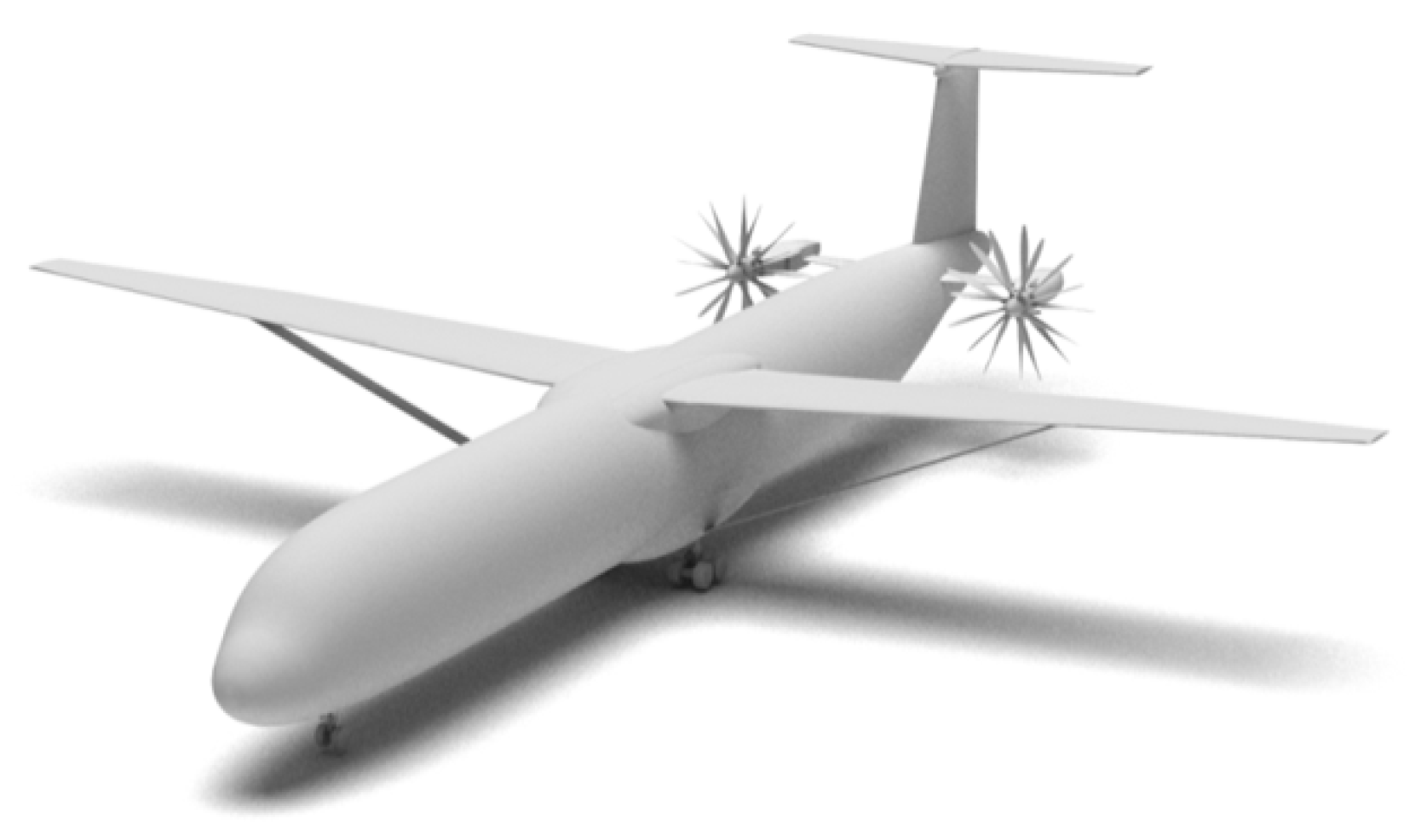
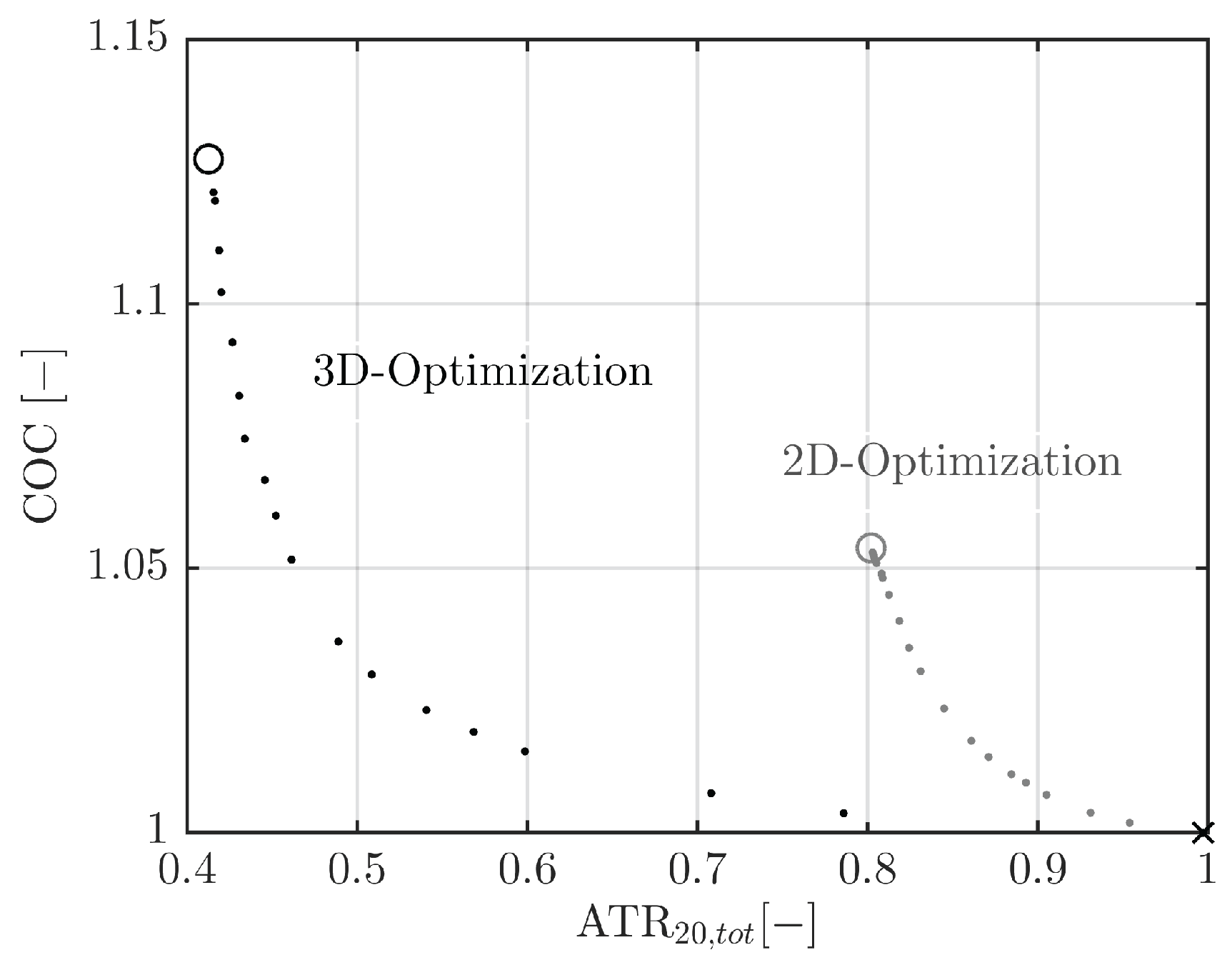
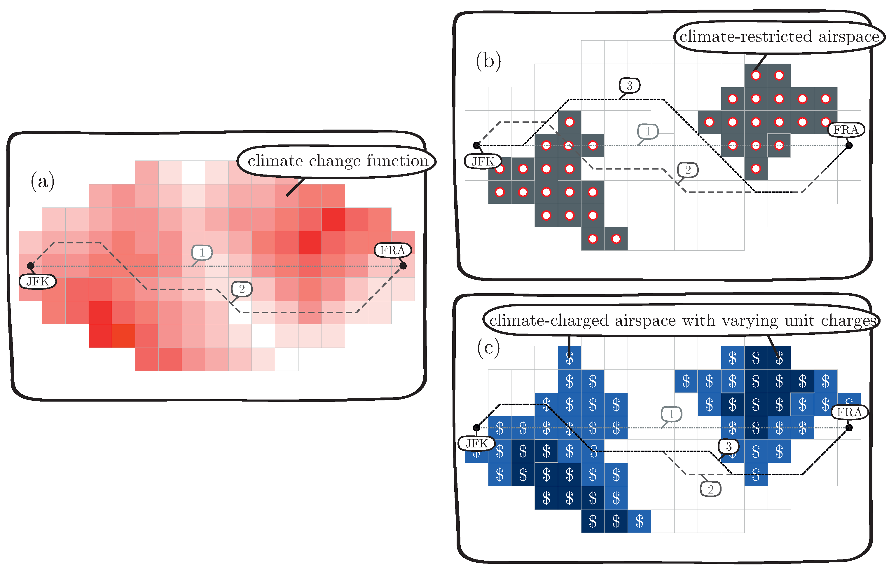
We assessed the climate impact of various technological and operational options and showed that a strut-braced wing aircraft with an open rotor has the potential to significantly reduce the climate impact, whereas intermediate stop operations, which have the potential to significantly reduce fuel consumption, will have an increased climate impact, since non-CO 2 effects compensate the reduced warming from CO 2 savings, if these operations are optimized for fuel use. Either a redesign of the aircraft or adapted aircraft trajectories would be necessary to achieve a lowered climate impact with ISO. Avoiding climate sensitive regions has a large potential in reducing climate impacts at relatively low costs. Full 3D optimization has a much better eco-efficiency than only lateral re-routings. The implementation of such operational measures requires, however, many more considerations, such as: is weather prediction accurate enough, how can we deal with uncertainties, e.g., in prognosing lifetimes and properties of contrails, is air traffic control in denser air traffic regions allowing for climate reduced trajectories, or what political and macro-economic framework is suited? Non-CO 2 effects are not considered in international agreements. We showed that if market-based measures were in place, which include these non-CO 2 effects, climate-optimal routing would be fostered. A measure that may be implemented on a more regional basis is closing air spaces which are very climate-sensitive. Although less effective than a free optimization, it still has a significant potential to reduce the climate impact of aviation.
We indicated that there are several open questions which require more research. One of them is the investigation of the aerosol-cloud feedbacks and alterations by aviation. An important point is the characterization of cruise particle emissions. Within WeCare we started a measurement campaign to characterize the particulate emissions in exhausts of aircraft engines, especially for new generation engines. This work is on-going and will be reported elsewhere. Here, we have concentrated on the impact of aviation aerosols on properties of low clouds. The impact of emitted soot particles on cirrus is an open issue and has potentially a large climate impact. There are new insights in other aviation related atmospheric processes available, making it seem appropriate to revise the overall climate impact of aviation, including estimates of the level of scientific understanding and including uncertainty ranges. The latter are important and should more rigorously be used in studies on the climate impact of mitigation options, providing uncertainty ranges and thereby giving more robust support in decision making. We showed that individual measures for mitigating the climate impact of aviation are hardly comparable since the framing conditions are very different. Therefore a roadmap would be required aiming at advising decision makers on time frames, requirements, and challenges for implementing measures.

Acknowledgments

Authors (except Andreas Zahn) obtained funding from the DLR-internal project WeCare.

Author Contributions

Volker Grewe and Katrin Dahlmann wrote the paper based on contributions from co-authors. Table 6 is giving the contribution details.
Table 6. Overview on author contributions. Section: Text contribution; Campaign: Performing the measurement campaign as well as performing a measurement during a campaign; Instrument: Development of an instrument used during the campaign; Model: Development of models or parts of models, Simulation: Perform a simulation, Data Analysis: Analysis of observational or model data.
NameSectionsCampaignInstrumentModelSimulationData Analysis
Volker Grewe2.2.3, 2.3.2, 2.2.3, 2.3.2 3.2, 4.3, 4.4, 4.5
3.2, 3.4,
4.3, 4.4, 4.5
Katrin Dahlmann2.2.3, 3.4 2.2.34.1, 4.3, 4.44.1, 4.3, 4.4
Jan Flink 2.2.1, 4.1
Christine Frömming 2.2.3, 3.2, 4.43.2, 4.3, 4.44.3
Robin Ghosh2.3.1 2.3.14.14.1
Klaus Gierens3.1 3.1
Romy Heller 2.1.12.1.1, 3.1 2.1.1, 3.1
Johannes Hendricks2.2.2, 3.3 2.2.2 3.3
Patrick Jöckel2.2.1 2.2.1, 2.2.2, 2.2.3, 3.22.2.3, 3.23.2
Stefan Kaufmann 2.1.12.1.1 2.1.1
Katrin Kölker 2.3.14.14.1
Florian Linke4.1, 4.2 2.3.1, 2.3.24.1, 4.2, 4.34.1, 4.2, 4.3, 4.4
Tanja Luchkova4.3 4.34.3
Benjamin Lührs2.3.2, 4.3 2.3.24.3, 4.44.3, 4.4
Jesper van Manen 4.4
Sigrun Matthes2.2.1, 3.2 2.2.13.23.2, 4.4
Andreas Minikin 2.1.12.1.1 3.1
Malte Niklaß4.4 2.3.24.44.4
Martin Plohr 2.3.1
Mattia Righi2.2.2, 3.3 2.2.23.33.3
Simon Rosanka 3.2
Angela Schmitt2.3.2 2.3.24.3
Ulrich Schumann2.1.1, 3.12.1.1 2.1.12.1.12.1.1
Ivan Terekhov 2.3.14.14.1
Simon Unterstrasser3.1 3.13.1
Margarita Vázquez-Navarro2.1.2, 3.12.1.1 3.1
Christiane Voigt2.1.1, 3.12.1.12.1.1, 3.1 2.1.1, 3.1
KaiWicke2.3.1 2.3.14.14.1
Hiroshi Yamashita2.3.2 2.3.22.3.22.3.2
Andreas Zahn 2.1.12.1.1
Helmut Ziereis3.22.1.12.1.1 3.2

Conflicts of Interest

The authors declare no conflict of interest. The founding sponsors had no role in the design of the study; in the collection, analyzes, or interpretation of data; in the writing of the manuscript, and in the decision to publish the results.

Abbreviations

The following abbreviations are used in this manuscript:
ACTAAutomatic Contrail Tracking Algorithm
ADISabre Airport Data Intelligence
AIRCASTAir Travel Forecast
AirTrafAir Traffic Submodel
ARMOGAAdaptive Range Multi-Objective Genetic Algorithm
ATRAverage Temperature Response
ATSAir Transportation System
BADABase of Aircraft Data
BAUBusiness as Usual Scenario
BCBlack Carbon
CCAClimate-Charged Airspace
CCFClimate Change Function
CiCContrail-induced Cloudiness
COCCash Operating Costs
COCSCirrus Optical Properties Derived from CALIOP and SEVIRI
CoCiPContrail and Cirrus Prediction Model
COSMOConsortium for Small-scale Modeling
COTClimate-Optimized Trajectories
CRAClimate-Restricted Airspace
CRORCouter Rotating Open Rotor
DLRDeutsches Zentrum für Luft- und Raumfahrt
ECHAMEuropean Centre Hamburg General Circulation Model
ECMWFEuropean Centre for Medium-Range Weather Forecasts
EMACECHAM/MESSy Atmospheric Chemistry Model
EULAGEuelerian/Lagrangian numerical solver
FFWDFast Foreward (fleet renewal model)
FIRFlight Information Region
FoAMForecast of Aircraft Movements
GRIDLABGlobal Air Traffic Emissions Distribution Laboratory
HALOHigh Altitude and Long Range Research Aircraft
ICAOInternational Civil Aviation Organization
IFInternational Future Global Modeling System
IPCCIntergovernmental Panel on Climate Change
ISOIntermediate Stop Operations
LCMLagrangian Cloud Model
LESLarge-Eddy Simulation
MADEModal Aerosol Dynamics for Europe
MBMMarket-Based Measures
MECO(n)Messy-fied ECHAM and COSMO Models nested n-times
MESSyModular Earth Submodel System
ML-CIRRUSMid-Latitude Cirrus Experiment
MSGMeteosat Second Generation
NAFCNorth Atlantic Flight Corridor
RCERemote Component Environment
REACT4CReducing Emissions from Aviation by Changing Trajectories for the Benefit of Climate
RFRadiative Forcing
SBWStrut-Braced Wing
TOMTrajectory Optimization Module
UTCUniversal Time Coordinated
WeCareUtilizing Weather information for climate efficient and eco efficient future aviation

References

  1. Lee, D.; Pitari, G.; Grewe, V.; Gierens, K.; Penner, J.; Petzold, A.; Prather, M.; Schumann, U.; Bais, A.; Berntsen, T.; et al. Transport impacts on atmosphere and climate: Aviation. Atmos. Environ. 2010, 44, 4678–4734. [Google Scholar] [CrossRef]
  2. Brasseur, G.P.; Gupta, M.; Anderson, B.E.; Balasubramanian, S.; Barrett, S.; Duda, D.; Fleming, G.; Forster, P.M.; Fuglestvedt, J.; Gettelman, A.; et al. Impact of Aviation on Climate: FAA’s Aviation Climate Change Research Initiative (ACCRI) Phase II. Bull. Am. Meteorol. Soc. 2016, 97, 561–583. [Google Scholar] [CrossRef]
  3. Fahey, D.W.; Lee, D.S. Aviation and Climate Change: A Scientific Perspective. Carbon Clim. Law Rev. 2016, 10, 97–104. [Google Scholar]
  4. Intergovernmental Panel on Climate Change (IPCC). Aviation and the Global Atmosphere: A Special Report of IPCC Working Groups I and III; Cambridge University Press: Cambridge, UK, 1999. [Google Scholar]
  5. Lee, D.; Fahey, D.; Forster, P.; Newton, P.; Wit, R.; Lim, L.; Owen, B.; Sausen, R. Aviation and global climate change in the 21st century. Atmos. Environ. 2009, 43, 3520–3537. [Google Scholar] [CrossRef]
  6. Holmes, C.; Tang, Q.; Prather, M. Uncertainties in climate assessment for the case of aviation NO. Proc. Natl. Acad. Sci. USA 2011, 108, 10997–11002. [Google Scholar] [CrossRef] [PubMed]
  7. Grewe, V.; Champougny, T.; Matthes, S.; Frömming, C.; Brinkop, S.; Sø vde, A.; Irvine, E.; Halscheidt, L. Reduction of the air traffic’s contribution to climate change: A REACT4C case study. Atmos. Environ. 2014, 94, 616–625. [Google Scholar] [CrossRef]
  8. Søvde, O.A.; Matthes, S.; Skowron, A.; Iachetti, D.; Lim, L.; Owen, B.; Hodnebrog, O.; Genova, G.D.; Pitari, G.; Lee, D.S.; et al. Aircraft emission mitigation by changing route altitude: A multi-model estimate of aircraft NOx emission impact on O3 photochemistry. Atmos. Environ. 2014, 95, 468–479. [Google Scholar] [CrossRef]
  9. Pitari, G.; Cionni, I.; Di Genova, G.; Søvde, O.A.; Lim, L. Radiative forcing from aircraft emissions of NOx: Model calculations with CH4 surface flux boundary condition. Meteorol. Z. 2016. [Google Scholar] [CrossRef]
  10. Myhre, G.; Shine, K.; Rädel, G.; Gauss, M.; Isaksen, I.; Tang, Q.; Prather, M.; Williams, J.; van Velthoven, P.; Dessens, O.; et al. Radiative forcing due to changes in ozone and methane caused by the transport sector. Atmos. Environ. 2011, 45, 387–394. [Google Scholar] [CrossRef]
  11. Grewe, V.; Dahlmann, K.; Matthes, S.; Steinbrecht, W. Attributing ozone to NOx emissions: Implications for climate mitigation measures. Atmos. Environ. 2012, 59, 102–107. [Google Scholar] [CrossRef]
  12. Appleman, H. The formation of exhaust condensation trails by the jet aircraft. Bull. Am. Meteorol. Soc. 1953, 34, 14–20. [Google Scholar]
  13. Schumann, U. On conditions for contrail formation from aircraft exhausts. Meterol. Z. 1996, 5, 4–23. [Google Scholar]
  14. Burkhardt, U.; Kärcher, B. Global radiative forcing from contrail cirrus. Nat. Clim. Chang. 2011, 1, 54–58. [Google Scholar] [CrossRef]
  15. Schumann, U.; Penner, J.E.; Chen, Y.; Zhou, C.; Graf, K. Dehydration effects from contrails in a coupled contrail-climate model. Atmos. Chem. Phys. 2015, 15, 11179–11199. [Google Scholar] [CrossRef]
  16. Intergovernmental Panel on Climate Change (IPCC). Climate Change 2013: The Physical Science Basis. Contribution of Working Group I to the Fifth Assessment Report of the Intergovernmental Panel on Climate Change; Cambridge University Press: Cambridge, UK; New York, NY, USA, 2013; p. 1535. [Google Scholar]
  17. Righi, M.; Hendricks, J.; Sausen, R. The global impact of the transport sectors on atmospheric aerosol: Simulations for year 2000 emissions. Atmos. Chem. Phys. 2013, 13, 9939–9970. [Google Scholar] [CrossRef]
  18. Wilcox, L.; Shine, K.; Hoskins, B. Radiative forcing due to aviation water vapour emissions. Atmos. Environ. 2012, 63, 1–13. [Google Scholar] [CrossRef]
  19. Hendricks, J.; Kärcher, B.; Lohmann, U.; Ponater, M. Do aircraft black carbon emissions affect cirrus clouds on the global scale? Geophys. Res. Lett. 2005, 32. [Google Scholar] [CrossRef]
  20. Hendricks, J.; Kärcher, B.; Lohmann, U. Effects of ice nuclei on cirrus clouds in a global climate model. J. Geophys. Res. 2011, 116, 1–24. [Google Scholar] [CrossRef]
  21. Gettelman, A.; Chen, C. The climate impact of aviation aerosols. Geophys. Res. Lett. 2013, 40, 2785–2789. [Google Scholar] [CrossRef]
  22. Zhou, C.; Penner, J.E. Aircraft soot indirect effect on large-scale cirrus clouds: Is the indirect forcing by aircraft soot positive or negative? J. Geophys. Res. 2014, 119, 11303–11320. [Google Scholar] [CrossRef]
  23. Airbus. Flying by numbers 2015–2034. In Global Market Forecast; Airbus: Toulouse, France, 2015. [Google Scholar]
  24. Schumann, U.; Graf, K.; Mannstein, H. Potential to reduce the climate impact of aviation by flight level changes. In Proceedings of the 3rd AIAA Atmospheric Space Environments Conference, Honolulu, HI, USA, 27–30 June 2011. No. 2011-3376. [Google Scholar]
  25. Matthes, S.; Schumann, U.; Grewe, V.; Frömming, C.; Dahlmann, K.; Koch, A.; Mannstein, H. Climate optimized air transport. In Atmospheric Physics: Background—Methods—Trends; Schumann, U., Ed.; Springer: Berlin/Heidelberg, Germany, 2012; pp. 727–746. [Google Scholar]
  26. Grewe, V.; Frömming, C.; Matthes, S.; Brinkop, S.; Ponater, M.; Dietmüller, S.; Jöckel, P.; Garny, H.; Dahlmann, K.; Tsati, E.; et al. Aircraft routing with minimal climate impact: The REACT4C climate cost function modelling approach (V1.0). Geosci. Model Dev. 2014, 7, 175–201. [Google Scholar] [CrossRef]
  27. Dahlmann, K.; Koch, A.; Linke, F.; Lührs, B.; Grewe, V.; Otten, T.; Seider, D.; Gollnick, V.; Schumann, U. Climate-Compatible Air Transport System—Climate Impact Mitigation Potential for Actual and Future Aircraft. Aerospace 2016, 3, 38. [Google Scholar] [CrossRef]
  28. Voigt, C.; Schumann, U.; Minikin, A.; Abdelmonem, A.; Afchine, A.; Borrmann, S.; Boettcher, M.; Buchholz, B.; Bugliaro, L.; Costa, A.; et al. ML-CIRRUS: The airborne experiment on natural cirrus and contrail cirrus with the high-altitude long-range research aircraft HALO. Bull. Am. Meteorol. Soc. 2017, 98, 271–288. [Google Scholar] [CrossRef]
  29. Schumann, U.; Heymsfield, A. On the lifecycle of individual contrails and contrail cirrus—Ice Formation and Evolution in Clouds and Precipitation: Measurement and Modeling Challenges: Chapter 3. Meteorol. Monogr. 2017, 58. [Google Scholar] [CrossRef]
  30. Groß, S.; Wirth, M.; Schäfler, A.; Fix, A.; Kaufmann, S.; Voigt, C. Potential of airborne lidar measurements for cirrus cloud studies. Atmos. Meas. Tech. 2014, 7, 2745–2755. [Google Scholar] [CrossRef]
  31. Schmetz, J.; Pili, P.; Tjemkes, S.; Just, D.; Kerkmann, J.; Rota, S.; Ratier, A. An introduction to Meteosat Second Generation (MSG). Bull. Am. Meteorol. Soc. 2002, 83, 977–997. [Google Scholar] [CrossRef]
  32. Vázquez-Navarro, M.; Mannstein, H.; Kox, S. Contrail life cycle and properties from 1 year of MSG/SEVIRI rapid-scan images. Atmos. Chem. Phys. 2015, 15, 8739–8749. [Google Scholar] [CrossRef]
  33. Schumann, U. A contrail cirrus prediction model. Geophys. Model Dev. 2012, 40, 543–580. [Google Scholar] [CrossRef]
  34. Voigt, C.; Jeßberger, P.; Jurkat, T.; Kaufmann, S.; Baumann, R.; Schlager, H.; Bobrowski, N.; Giuffrida, G.; Salerno, G. Evolution of CO2, SO2, HCl, and HNO3 in the volcanic plumes from Etna. Geophys. Res. Lett. 2014, 41, 2196–2203. [Google Scholar] [CrossRef]
  35. Vázquez-Navarro, M.; Mannstein, H.; Mayer, B. An automatic contrail tracking algorithm. Atmos. Meas. Tech. 2010, 3, 1089–1101. [Google Scholar] [CrossRef]
  36. Mannstein, H.; Meyer, R.; Wendling, P. Operational Detection of Contrails from NOAA-AVHRR-Data. Int. J. Remote Sens. 1999, 20, 1641–1660. [Google Scholar] [CrossRef]
  37. Grewe, V.; Moussiopoulos, N.; Builtjes, P.; Borrego, C.; Isaksen, I.S.A.; Volz-Thomas, A. The ACCENT-protocol: A framework for benchmarking and model evaluation. Geophys. Model Dev. 2012, 5, 611–618. [Google Scholar] [CrossRef]
  38. Jöckel, P.; Tost, H.; Pozzer, A.; Kunze, M.; Kirner, O.; Brenninkmeijer, C.A.M.; Brinkop, S.; Cai, D.S.; Dyroff, C.; Eckstein, J.; et al. Earth System Chemistry integrated Modelling (ESCiMo) with the Modular Earth Submodel System (MESSy) version 2.51. Geosci. Model Dev. 2016, 9, 1153–1200. [Google Scholar] [CrossRef]
  39. Kerkweg, A.; Jöckel, P. The 1-way on-line coupled atmospheric chemistry model system MECO(n) —Part 1: Description of the limited-area atmospheric chemistry model COSMO/MESSy. Geosci. Model Dev. 2012, 5, 87–110. [Google Scholar] [CrossRef]
  40. Kerkweg, A.; Jöckel, P. The 1-way on-line coupled atmospheric chemistry model system MECO(n)—Part 2: On-line coupling with the Multi-Model-Driver (MMD). Geosci. Model Dev. 2012, 5, 111–128. [Google Scholar] [CrossRef]
  41. Mertens, M.; Kerkweg, A.; Jöckel, P.; Tost, H.; Hofmann, C. The 1-way on-line coupled model system MECO(n)—Part 4: Chemical evaluation (based on MESSy v2.52). Geosci. Model Dev. 2016, 9, 3545–3567. [Google Scholar] [CrossRef]
  42. Lauer, A.; Hendricks, J.; Ackermann, I.J.; Schell, B.; Hass, H.; Metzger, S. Simulating aerosol microphysics with the ECHAM/MADE GCM—Part I: Model description and comparison with observations. Atmos. Chem. Phys. 2005, 5, 3251–3276. [Google Scholar] [CrossRef]
  43. Kaiser, J.C.; Hendricks, J.; Righi, M.; Riemer, N.; Zaveri, R.A.; Metzger, S.; Aquila, V. The MESSy aerosol submodel MADE3 (v2.0b): Description and a box model test. Geosci. Model Dev. 2014, 7, 1137–1157. [Google Scholar] [CrossRef]
  44. Hoose, C.; Möhler, O. Heterogeneous ice nucleation on atmospheric aerosols: A review of results from laboratory experiments. Atmos. Chem. Phys. 2012, 12, 9817–9854. [Google Scholar] [CrossRef]
  45. Kuebbeler, M.; Lohmann, U.; Hendricks, J.; Kärcher, B. Dust ice nuclei effects on cirrus clouds. Atmos. Chem. Phys. 2014, 14, 3027–3046. [Google Scholar] [CrossRef]
  46. Kärcher, B.; Hendricks, J.; Lohmann, U. Physically based parameterization of cirrus cloud formation for use in global atmospheric models. J. Geophys. Res. 2006, 111, D01205. [Google Scholar] [CrossRef]
  47. Jöckel, P.; Kerkweg, A.; Pozzer, A.; Sander, R.; Tost, H.; Riede, H.; Baumgaertner, A.; Gromov, S.; Kern, B. Development cycle 2 of the modular earth submodel system (MESSy2). Geosci. Model Dev. 2010, 3, 717–752. [Google Scholar] [CrossRef]
  48. Dahlmann, K.; Grewe, V.; Frömming, C.; Burkhardt, U. Can we reliably assess climate mitigation options for air traffic scenarios despite large uncertainties in atmospheric processes? Transp. Res. Part D Transp. Environ. 2016, 46, 40–55. [Google Scholar] [CrossRef]
  49. Grewe, V.; Stenke, A. AirClim: An efficient climate impact assessment tool. Atmos. Chem. Phys. 2008, 8, 4621–4639. [Google Scholar] [CrossRef]
  50. Niklaß, M.; Lührs, B.; Grewe, V.; Dahlmann, K.; Luchkova, T.; Linke, F.; Gollnick, V. Potential to reduce the climate impact of aviation by climate restricted airspaces. Transp. Policy 2017, in press. [Google Scholar]
  51. Marquart, S.; Ponater, M.; Mager, F.; Sausen, R. Future Development of Contrail Cover, Optical Depth, and Radiative Forcing: Impacts of Increasing Air Traffic and Climate Change. J. Clim. 2003, 16, 2890–2904. [Google Scholar] [CrossRef]
  52. Ghosh, R.; Kölker, K.; Terekhov, T. Future passenger air traffic modelling: A theoretical concept to integrate quality of travel, cost of travel and capacity constraints. In Proceedings of the 19th World Conference of the Air Transport Research Society (ATRS), Singapore, 2–4 July 2015. [Google Scholar]
  53. Ghosh, R.; Wicke, K.; Kölker, K.; Terekhov, I.; Linke, F.; Niklaß, M.; Lührs, B.; Grewe, V. An integrated modelling approach for climate impact assessments in the future air transportation system—Findings from the WeCare project. In Proceedings of the 2nd ECATS Conference, Athens, Greece, 7–9 November 2016. [Google Scholar]
  54. Terekhov, I.; Ghosh, R.; Gollnick, V. A concept of forecasting origin-destination air passenger demand between global city pairs using future socio-economic development scenarios. In Proceedings of the 53rd AIAA Aerospace Sciences Meeting, Kissimmee, FL, USA, 5–9 January 2015. [Google Scholar]
  55. Terekhov, I.; Evans, A.; Gollnick, V. Forecasting a global air passenger demand network using weighted similarity-based algorithms. In Complex Networks VII; Springer: Berlin/Heidelberg, Germany, 2016; pp. 335–347. [Google Scholar]
  56. Randers, J. 2052: A Global Forecast for the Next Forty Years; Chelsea Green Publishing: White River Junction, VT, USA, 2012. [Google Scholar]
  57. Hughes, B.; Hillebrand, E. Exploring and Shaping International Futures; Paradigm Publishers: New York, NY, USA, 2006. [Google Scholar]
  58. Kölker, K.; Bießlich, P.; Lütjens, K. From passenger growth to aircraft movements. J. Air Transp. Manag. 2016, 56, 99–106. [Google Scholar] [CrossRef]
  59. Apffelstaedt, A.; Langhans, S.; Gollnick, V. Identifying carbon dioxide reducing aircraft technologies and estimating their impact on global CO2 emissions. In Proceedings of the Deutscher Luft- und Raumfahrt Kongress (DLRK), Aachen, Germany, 8–10 September 2009. [Google Scholar]
  60. Kölker, K.; Ghosh, R.; Lütjens, K. Assessing quality of air travel using the impact of frequency, travel time and transfers on passenger demand. In Proceedings of the 19th World Conference of the Air Transport Research Society (ATRS), Singapore, 2–4 July 2015. [Google Scholar]
  61. Linke, F. Ökologische Analyse Operationeller Lufttransportkonzepte. Ph.D. Thesis, Hamburg University of Technology (TUHH), Hamburg, Germany, 2016. [Google Scholar]
  62. Seider, D.; Fischer, P.; Litz, M.; Schreiber, A.; Gerndt, A. Open Source Software Framework for Applications in Aeronautics and Space. In Proceedings of the IEEE Aerospace Conference, Big Sky, MT, USA, 3–10 March 2012. [Google Scholar]
  63. Koch, A.; Lührs, B.; Dahlmann, K.; Linke, F.; Grewe, V.; Litz, M.; Plohr, M.; Nagel, B.; Gollnick, V.; Schumann, U. Climate impact assessment of varying cruise flight altitudes applying the CATS simulation approach. In Proceedings of the International Conference of the European Aerospace Societies (CEAS), Venice, Italy, 24–28 October 2011. [Google Scholar]
  64. Ghosh, R.; Schilling, T.; Wicke, K. Theoretical framework of systems design for the air transportation system including an inherently quantitative philosophy of scenario development. J. Air Transp. Manag. 2017, 58, 58–67. [Google Scholar] [CrossRef]
  65. Ghosh, R.; Terekhov, I. Future passenger air traffic modelling: Trend analysis of the global passenger air travel demand network. In Proceedings of the 53rd AIAA Aerospace Sciences Meeting, Kissimmee, FL, USA, 5–12 January 2015. [Google Scholar]
  66. Lührs, B.; Niklaß, M.; Frömming, C.; Grewe, V.; Gollnick, V. Cost-Benefit Assessment of 2D and 3D Climate and Weather Optimized Trajectories. In Proceedings of the 16th AIAA Aviation Technology, Integration, and Operations Conference, Washington, DC, USA, 13–17 June 2016. [Google Scholar]
  67. Nuic, A.; Mouillet, V. User Manual for the Base of Aircraft Data (BADA) Family 4; Technical Report 12/11/22-58; Eurocontrol, Experimental Centre: Brétigny-sur-Orge, France, 2012. [Google Scholar]
  68. DuBois, D.; Paynter, G.C. “Fuel Flow Method2” for Estimating Aircraft Emissions; SAE Technical Paper; SAE International: Warrendale, PA, USA, 2006. [Google Scholar]
  69. Jelinik, F.; Carlier, S.; Smith, J. Advanced Emission Model (AEM3) v1.5; Technical Report EEC/SEE/2004/004; Eurocontrol, Experimental Centre: Brétigny-sur-Orge, France, 2004. [Google Scholar]
  70. Nuic, A. User Manual for the Base of Aircraft Data (BADA) Revision 3.9; EEC Technical/Scientific Report No.12/04/10-45; Eurocontrol, Experimental Centre: Brétigny-sur-Orge, France, 2011. [Google Scholar]
  71. Zillies, J.; Schmitt, A.R.; Vujasinovic, R. Multiobjective 4D optimization of a trajectory-based air traffic management. In Proceedings of the Integrated Communications, Navigation and Surveillance Conference (ICNS), Herndon, VA, USA, 23–25 April 2013; pp. 1–11. [Google Scholar]
  72. Zillies, J.; Kuenz, A.; Schmitt, A.; Schwoch, G.; Mollwitz, V.; Edinger, C. Wind optimized routing: An opportunity to improve european flight efficiency? In Proceedings of the IEEE Integrated Communications, Navigation and Surveillance Conference (ICNS), Herndon, VA, USA, 8–10 April 2014; pp. X3-1–X3-9. [Google Scholar]
  73. Yamashita, H.; Grewe, V.; Jöckel, P.; Linke, F.; Schaefer, M.; Sasaki, D. Air traffic simulation in chemistry-climate model EMAC 2.41: AirTraf 1.0. Geosci. Model Dev. 2016, 9, 3363–3392. [Google Scholar] [CrossRef]
  74. International Civil Aviation Organization (ICAO). ICAO Engine Exhaust Emissions Data; Technical Report, Doc 9646-AN/943 (Issue 18); International Civil Aviation Organization: Montreal, QC, Canada, 2005. [Google Scholar]
  75. Sasaki, D.; Obayashi, S.; Nakahashi, K. Navier-Stokes optimization of supersonic wings with four objectives using evolutionary algorithm. J. Aircr. 2002, 39, 621–629. [Google Scholar] [CrossRef]
  76. Sasaki, D.; Obayashi, S. Efficient search for trade-offs by adaptive range multi-objective genetic algorithms. J. Aerosp. Comput. Inf. Commun. 2005, 2, 44–64. [Google Scholar] [CrossRef]
  77. Schaefer, M. Development of Forecast Model for Global Air Traffic Emissions. Ph.D. Thesis, Deutsches Zentrum für Luft-und Raumfahrt (DLR), Köln, Germany, 2012. [Google Scholar]
  78. Deidewig, F.; Döpelheuer, A.; Lecht, M. Methods to assess aircraft engine emissions in flight. In ICAS PROCEEDINGS; International Council of the Aeronautical Sciences: Sorrent, Italy, 1996; Volume 20, pp. 131–141. [Google Scholar]
  79. Yamashita, H.; Grewe, V.; Jöckel, P.; Linke, F.; Schaefer, M.; Sasaki, D. Towards Climate Optimized Flight Trajectories in a Climate Model: AirTraf. 2015. Available online: http://www.atmseminar.org/seminarContent/seminar11/papers/433-yamashita_0126151229-Final-Paper-5-6-15.pdf (accessed on 1 July 2015).
  80. Frömming, C.; Grewe, V.; Jöckel, P.; Brinkop, S.; Dietmüller, S.; Garny, H.; Ponater, M.; Tsati, E.; Matthes, S. Climate Cost Functions as Basis for Climate Optimized Flight Trajectories. 2013. Available online: http://www.atmseminar.org/seminarContent/seminar10/papers/239-Frömming_0126130830-Final-Paper-4-15-13.pdf (accessed on 27 January 2015).
  81. Frömming, C.; Grewe, V.; Brinkop, S.; Haslerud, A.; Matthes, S.; Irvine, E.; Rosanka, S.; van Manen, J. Influence of weather situations on aviation emission effcts: The REACT4C Climate Change Functions. Atmos. Environ. 2017. in preparation. [Google Scholar]
  82. Jeßberger, P.; Voigt, C.; Schumann, U.; Sölch, I.; Schlager, H.; Kaufmann, S.; Petzold, A.; Schäuble, D.; Gayet, J.F. Aircraft type influence on contrail properties. Atmos. Chem. Phys. 2013, 13, 11965–11984. [Google Scholar] [CrossRef]
  83. Ziereis, H.; Schlager, H.; Schulte, P.; van Velthoven, P.; Slemr, F. Distributions of NO, NOx , and NOy in the upper troposphere and lower stratosphere between 28° and 61° N during POLINAT 2. J. Geophys. Res. 2000, 105, 3653–3664. [Google Scholar] [CrossRef]
  84. Jurkat, T.; Voigt, C.; Arnold, F.; Schlager, H.; Kleffmann, J.; Aufmhoff, H.; Schäuble, D.; Schaefer, M.; Schumann, U. Measurements of HONO, NO, NOy and SO2 in aircraft exhaust plumes at cruise. Geophys. Res. Lett. 2011, 38. [Google Scholar] [CrossRef]
  85. Voigt, C.; Schumann, U.; Jeßberger, P.; Jurkat, T.; Petzold, A.; Gayet, J.F.; Krämer, M.; Thornberry, T.; Fahey, D.W. Extinction and optical depth of contrails. Geophys. Res. Lett. 2011, 38, L11806. [Google Scholar] [CrossRef]
  86. Voigt, C.; Schumann, U.; Jurkat, T.; Schäuble, D.; Schlager, H.; Petzold, A.; Gayet, J.F.; Krämer, M.; Schneider, J.; Borrmann, S.; et al. In-situ observations of young contrails: Overview and selected results from the CONCERT campaign. Atmos. Chem. Phys. 2010, 10, 9039–9056. [Google Scholar] [CrossRef]
  87. Schumann, U.; Schlager, H.; Arnold, F.; Baumann, R.; Haschberger, P.; Klemm, O. Dilution of aircraft exhaust plumes at cruise altitudes. Atmos. Environ. 1998, 32, 3097–3103. [Google Scholar] [CrossRef]
  88. Schröder, F.; Kärcher, B.; Duroure, C.; Strom, J.; Petzold, A.; Gayet, J.F.; Strauss, B.; Wendling, P.; Borrmann, S. On the transition of contrails into cirrus clouds. J. Atmos. Sci. 2000, 57, 464–480. [Google Scholar] [CrossRef]
  89. Gayet, J.F.; Shcherbakov, V.; Voigt, C.; Schumann, U.; Schäuble, D.; Jeßberger, P.; Petzold, A.; Minikin, A.; Schlager, H.; Dubovik, O.; et al. The evolution of microphysical and optical properties of an A380 contrail in the vortex phase. Atmos. Chem. Phys. 2012, 12, 6629–6643. [Google Scholar] [CrossRef]
  90. Schumann, U.; Jeßberger, P.; Voigt, C. Contrail ice particles in aircraft wakes and their climatic importance. Geophys. Res. Lett. 2013, 40, 2867–2872. [Google Scholar] [CrossRef]
  91. Kaufmann, S.; Voigt, C.; Jeßberger, P.; Jurkat, T.; Schlager, H.; Schwarzenboeck, A.; Klingebiel, M.; Thornberry, T. In situ measurements of ice saturation in young contrails. Geophys. Res. Lett. 2014, 41, 702–709. [Google Scholar] [CrossRef]
  92. Schumann, U.; Baumann, R.; Baumgardner, D.; Bedka, S.; Duda, D.; Freudenthaler, V.; Gayet, J.F.; Heymsfield, A.J.; Minnis, P.; Quante, M.; et al. Properties of individual contrails: A compilation of observations and some comparisons. Atmos. Chem. Phys. 2017, 17, 403–438. [Google Scholar] [CrossRef]
  93. Kox, S.; Bugliaro, L.; Ostler, A. Retrieval of cirrus cloud optical thickness and top altitude from geostationary remote sensing. Atmos. Meas. Tech. Discuss. 2014, 7, 4123–4161. [Google Scholar] [CrossRef]
  94. Iwabuchi, H.; Yang, P.; Liou, K.N.; Minnis, P. Physical and optical properties of persistent contrails: Climatology and interpretation. J. Geophys. Res. 2012, 117. [Google Scholar] [CrossRef]
  95. Bedka, S.T.; Minnis, P.; Duda, D.P.; Chee, T.L.; Palikonda, R. Properties of linear contrails in the Northern Hemisphere derived from 2006 Aqua MODIS observations. Geophys. Res. Lett. 2013, 40, 772–777. [Google Scholar] [CrossRef]
  96. Vázquez-Navarro, M.; Mayer, B.; Mannstein, H. A fast method for the retrieval of integrated longwave and shortwave top-of-atmosphere upwelling irradiances from MSG/SEVIRI (RRUMS). Atmos. Meas. Tech. 2013, 6, 2627–2640. [Google Scholar] [CrossRef]
  97. Stuber, N.; Forster, P. The impact of diurnal variations of air traffic on contrail radiative forcing. Atmos. Chem. Phys. 2007, 7, 3153–3162. [Google Scholar] [CrossRef]
  98. Meerkötter, R.; Schumann, U.; Doelling, D.R.; Minnis, P.; Nakajima, T.; Tsushima, Y. Radiative forcing by contrails. Ann. Geophys. 1999, 17, 1080–1094. [Google Scholar] [CrossRef]
  99. Palikonda, R.; Minnis, P.; Duda, D. Contrail climatology over the USA from MODIS and AVHRR data. In Proceedings of the AMS 10th Conference Aviation, Range, and Aerospace Meteor, Portland, OR, USA, 13–16 May 2002. [Google Scholar]
  100. Prusa, J.; Smolarkiewicz, P.; Wyszogrodzki, A. EULAG, a computational model for multiscale flows. Comput. Fluids 2008, 37, 1193–1207. [Google Scholar] [CrossRef]
  101. Sölch, I.; Kärcher, B. A large-eddy model for cirrus clouds with explicit aerosol and ice microphysics and Lagrangian ice particle tracking. Q. J. R. Meteorol. Soc. 2010, 136, 2074–2093. [Google Scholar] [CrossRef]
  102. Unterstrasser, S.; Sölch, I. Optimisation of simulation particle number in a Lagrangian ice microphysical model. Geophys. Mod. Dev. 2014, 7, 695–709. [Google Scholar] [CrossRef]
  103. Unterstrasser, S. Large eddy simulation study of contrail microphysics and geometry during the vortex phase and consequences on contrail-to-cirrus transition. J. Geophys. Res. 2014, 119, 7537–7555. [Google Scholar] [CrossRef]
  104. Unterstrasser, S.; Paoli, R.; Sölch, I.; Kühnlein, C.; Gerz, T. Dimension of aircraft exhaust plumes at cruise conditions: Effect of wake vortices. Atmos. Chem. Phys. 2014, 14, 2713–2733. [Google Scholar] [CrossRef]
  105. Unterstrasser, S.; Görsch, N. Aircraft-type dependency of contrail evolution. J. Geophys. Res. 2014, 119, 14015–14027. [Google Scholar] [CrossRef]
  106. Unterstrasser, S.; Gierens, K. Numerical simulations of contrail-to-cirrus transition—Part 1: An extensive parametric study. Atmos. Chem. Phys. 2010, 10, 2017–2036. [Google Scholar] [CrossRef]
  107. Unterstrasser, S. Properties of young contrails—A parametrisation based on large-eddy simulations. Atmos. Chem. Phys. 2016, 16, 2059–2082. [Google Scholar] [CrossRef]
  108. Unterstrasser, S.; Gierens, K.; Sölch, I.; Lainer, M. Numerical simulations of homogeneously nucleated natural cirrus and contrail-cirrus. Part 1: How different are they? Meteorol. Z. 2016, 1–22. [Google Scholar] [CrossRef]
  109. Unterstrasser, S.; Gierens, K.; Sölch, I.; Wirth, M. Numerical simulations of homogeneously nucleated natural cirrus and contrail-cirrus. Part 2: Interaction on local scale. Meteorol. Z. 2016, 1–19. [Google Scholar] [CrossRef]
  110. Schumann, U.; Graf, K. Aviation-induced cirrus and radiation changes at diurnal timescales. J. Geophys. Res. 2013, 118, 2404–2421. [Google Scholar] [CrossRef]
  111. Bock, L.; Burkhardt, U. Reassessing properties and radiative forcing of contrail cirrus using a climate model. J. Geophys. Res. 2016, 121, 9717–9736. [Google Scholar] [CrossRef]
  112. Gierens, K.; Dilger, F. A climatology of formation conditions for aerodynamic contrails. Atmos. Chem. Phys. 2013, 13, 10847–10857. [Google Scholar] [CrossRef]
  113. Kärcher, B.; Mayer, B.; Gierens, K.; Burkhardt, U.; Mannstein, H.; Chatterjee, R. Aerodynamic contrails: Microphysics and optical properties. J. Atmos. Sci. 2009, 66, 227–243. [Google Scholar] [CrossRef]
  114. Jansen, J.; Heymsfield, A. Microphysics of aerodynamic contrail formation processes. J. Atmos. Sci. 2015, 72, 3293–3308. [Google Scholar] [CrossRef]
  115. Gierens, K.; Kästner, M.; Klatt, D. Iridescent aerodynamic contrails: The Norderney case of 27 June 2008. Meteorol. Z. 2011, 20, 305–311. [Google Scholar] [CrossRef]
  116. Zahn, A.; Weppner, J.; Widmann, H.; Schlote-Holubek, K.; Burger, B.; Kühner, T.; Franke, H. A fast and precise chemiluminescence ozone detector for eddy flux and airborne application. Atmos. Meas. Tech. 2012, 5, 363–375. [Google Scholar] [CrossRef]
  117. Köhler, M.O.; Rädel, G.; Dessens, O.; Shine, K.; Rogers, H.; Wild, O.; Pyle, J. Impact of perturbations to nitrogen oxide emissions from global aviation. J. Geophys. Res. 2008, 113, D11305. [Google Scholar] [CrossRef]
  118. Stevenson, D.; Derwent, R. Does the location of aircraft nitrogen oxide emissions affect their climate impact? Geophys. Res. Lett. 2009, 36, L17810. [Google Scholar] [CrossRef]
  119. Stevenson, D.; Doherty, R.; Sanderson, M.; Collins, W.; Johnson, C.; Derwent, R.G. Radiative forcing from aircraft NOx emissions: Mechanisms and seasonal dependence. J. Geophys. Res. 2004, 109, D17307. [Google Scholar] [CrossRef]
  120. Hoor, P.; Borken-Kleefeld, J.; Caro, D.; Dessens, O.; Endresen, O.; Gauss, M.; Grewe, V.; Hauglustaine, D.; Isaksen, I.S.A.; Jöckel, P.; et al. The impact of traffic emissions on atmospheric ozone and OH: Results from QUANTIFY. Atmos. Chem. Phys. 2009, 9, 3113–3136. [Google Scholar] [CrossRef]
  121. Grewe, V.; Tsati, E.; Hoor, P. On the attribution of contributions of atmospheric trace gases to emissions in atmospheric model applications. Geophys. Model Dev. 2010, 3, 487–499. [Google Scholar] [CrossRef]
  122. Deckert, R.; Jöckel, P.; Grewe, V.; Gottschaldt, K.D.; Hoor, P. A quasi chemistry-transport model mode for EMAC. Geophys. Model Dev. 2011, 4, 195–206. [Google Scholar] [CrossRef]
  123. Lamarque, J.F.; Bond, T.C.; Eyring, V.; Granier, C.; Heil, A.; Klimont, Z.; Lee, D.S.; Liousse, C.; Mieville, A.; Owen, B.; et al. Historical (1850–2000) gridded anthropogenic and biomass burning emissions of reactive gases and aerosols: Methodology and application. Atmos. Chem. Phys. 2010, 10, 7017–7039. [Google Scholar] [CrossRef]
  124. Moss, R.H.; Edmonds, J.A.; Hibbard, K.A.; Manning, M.R.; Rose, S.K.; van Vuuren, D.P.; Carter, T.R.; Emori, S.; Kainuma, M.; Kram, T.; et al. The next generation of scenarios for climate change research and assessment. Nature 2010, 463, 747–756. [Google Scholar] [CrossRef] [PubMed]
  125. Righi, M.; Hendricks, J.; Sausen, R. The global impact of the transport sectors on atmospheric aerosol in 2030—Part 2: Aviation. Atmos. Chem. Phys. 2016, 16, 4481–4495. [Google Scholar] [CrossRef]
  126. Lohmann, U.; Feichter, J. Global indirect aerosol effect: A review. Atmos. Chem. Phys. 2005, 5, 715–737. [Google Scholar] [CrossRef]
  127. Kapadia, Z.Z.; Spracklen, D.V.; Arnold, S.R.; Borman, D.J.; Mann, G.W.; Pringle, K.J.; Monks, S.A.; Reddington, C.L.; Benduhn, F.; Rap, A.; et al. Impacts of aviation fuel sulfur content on climate and human health. Atmos. Chem. Phys. 2016, 16, 10521–10541. [Google Scholar] [CrossRef]
  128. Schumann, U.; Arnold, F.; Busen, R.; Curtius, J.; Kärcher, B.; Kiendler, A.; Petzold, A.; Schlager, H.; Schröder, F.; Wohlfrom, K.H. Influence of fuel sulfur on the composition of aircraft exhaust plumes: The experiments SULFUR 1–7. J. Geophys. Res. 2002, 107, AAC 2-1–AAC 2-27. [Google Scholar] [CrossRef]
  129. Unger, N.; Zhao, Y.; Dang, H. Mid-21st century chemical forcing of climate by the civil aviation sector. Geophys. Res. Lett. 2013, 40, 641–645. [Google Scholar] [CrossRef]
  130. Unger, N. Global climate impact of civil aviation for standard and desulfurized jet fuel. Geophys. Res. Lett. 2011, 38. [Google Scholar] [CrossRef]
  131. Fuglestvedt, J.; Shine, K.; Berntsen, T.; Cook, J.; Lee, D.; Stenke, A.; Skeie, R.; Velders, G.; Waitz, I. Transport impacts on atmosphere and climate: Metrics. Atmos. Environ. 2015, 44, 4648–4677. [Google Scholar] [CrossRef]
  132. Grewe, V.; Dahlmann, K. How ambiguous are climate metrics? And are we prepared to assess and compare the climate impact of new air traffic technologies? Atmos. Environ. 2015, 106, 373–374. [Google Scholar] [CrossRef]
  133. Sanchez Barreda, V.J. Conceptual Design Optimization of a Strut Braced Wing Aircraft. Master’s Thesis, Hamburg University of Applied Sciences, Hamburg, Germany, 2013. [Google Scholar]
  134. Plohr, M. Anwendungsorientierte Methoden zur Analyse und Modellierung des Emissionsverhaltens Moderner Triebwerke Mit Gestuften, Mageren Brennkammersystemen auf Basis Thermodynamischer Triebwerksmodelle. Ph.D. Thesis, Ruhr-Universität Bochum, Bochum, Germany, 2015. [Google Scholar]
  135. Linke, F.; Lührs, B.; Grewe, V.; Kölker, K.; Ghosh, R.; Terekhov, I.; Niklaß, M.; Wicke, K.; Dahlmann, K.; Plohr, M.; et al. The expected impact from the introduction of a new Strut-Braced Wing aircraft configuration on global air traffic emissions and climate: Results from the WeCare project. In Proceedings of the 2nd Environmentally Compatible Air Transport System Conference ECATS 2016, Athen, Griechenland, 7–9 November 2016. [Google Scholar]
  136. Kärcher, B.; Yu, F. Role of aircraft soot emissions in contrail formation. Geophys. Res. Lett. 2009, 36, L01804. [Google Scholar] [CrossRef]
  137. Kärcher, B.; Burkhardt, U.; Bier, A.; Bock, L.; Ford, I.J. The microphysical pathway to contrail formation. J. Geophys. Res. 2015, 120, 7893–7927. [Google Scholar] [CrossRef]
  138. Zhang, Y.; Macke, A.; Albers, F. Effect of crystal size spectrum and crystal shape on stratiform cirrus radiative forcing. Atmos. Res. 1999, 52, 59–75. [Google Scholar] [CrossRef]
  139. Martinez-Val, R.; Roa, J.; Perez, E.; Cuerno, C. Effects of the Mismatch Between Design Capabilities and Actual Aircraft Utilization. J. Aircr. 2011, 48, 1921–1927. [Google Scholar] [CrossRef]
  140. Lammering, T.; Anton, E.; Risse, K.; Franz, K.; Hoernschemeyer, R. Gains in Fuel Efficiency: Multi-Stop Missions vs. Laminar Aircraft. In Proceedings of the 11th Aviation Technology, Integration, and Operations (ATIO) Conference, Virginia Beach, VA, USA, 20–22 September 2011. [Google Scholar]
  141. Langhans, S.; Linke, F.; Nolte, P.; Schnieder, H. System analysis for future long-range operation concepts. In Proceedings of the 27th Congress of the International Council of the Aeronautical Sciences (ICAS), Nice, France, 19–24 September 2010. [Google Scholar]
  142. Creemers, W.; Slingerland, R. Impact of Intermediate Stops on Long-Range Jet-Transport Design. In Proceedings of the 7th AIAA Aviation Technology, Integration and Operations (ATIO) Conference, Belfast, Northern Ireland, 18–20 September 2007. [Google Scholar]
  143. Poll, D.I.A. On the effect of stage length on the efficiency of air transport. Aeronaut. J. 2011, 115, 273–283. [Google Scholar] [CrossRef]
  144. Green, J.E. Air Travel—Greener by Design: Mitigating the Environmental Impact of Aviation: Opportunities and Priorities; Technical Report, Report of the Science and Technology Sub-Group; Royal Aeronautical Society: London, UK, 2005. [Google Scholar]
  145. Linke, F.; Langhans, S.; Gollnick, V. Global Fuel Analysis of Intermediate Stop Operations on Long-Haul Routes. In Proceedings of the 11th Aviation Technology, Integration, and Operations (ATIO) Conference, Virginia Beach, VA, USA, 20–22 September 2011. [Google Scholar]
  146. Linke, F.; Grewe, V.; Gollnick, V. The Implications of Intermediate Stop Operations on Aviation Emissions and Climate. Meteorol. Z. 2017. [Google Scholar] [CrossRef]
  147. Sausen, R.; Nodorp, D.; Land, C. Towards an optimal flight routing with respect to minimal environmental impact. In Impact of Emissions from Aircraft and Spacecraft upon the Atmosphere; Schumann, U., Wurzel, D., Eds.; DLR: Cologne, Germany, 1994; pp. 473–478. [Google Scholar]
  148. Mannstein, H.; Spichtinger, P.; Gierens, K. A note on how to avoid contrail cirrus. Transp. Res. 2005, 10, 421–426. [Google Scholar] [CrossRef]
  149. Sridhar, B.; Ng, H.; Chen, N. Integration of Linear Dynamic Emission and Climate Models with Air Traffic Simulations. In Proceedings of the AIAA Guidance, Navigation and Control Conference, Minneapolis, MN, USA, 13–16 August 2012. [Google Scholar]
  150. Lührs, B.; Linke, F.; Gollnick, V. Erweiterung eines Trajektorienrechners zur Nutzung meteorologischer Daten für die Optimierung von Flugzeugtrajektorien. In Proceedings of the Deutscher Luft- und Raumfahrtkongress (DLRK), Augsburg, Germany, 16–18 September 2014. [Google Scholar]
  151. Grewe, V.; Matthes, S.; Frömming, C.; Brinkop, S.; Jöckel, P.; Gierens, K.; Champougny, T.; Fuglestvedt, J.; Haslerud, A.; Irvine, E.; et al. Feasibility of climate-optimized air traffic routing for trans-Atlantic flights. Environ. Res. Lett. 2017, 12, 034003. [Google Scholar] [CrossRef]
  152. Kreuz, M.; Luchkova, T.; Schultz, M. Effect of Restricted Airspace on the ATM System. In Proceedings of the World Conference on Transport Research (WCTR 2016), Shanghai, China, 10–15 July 2016. [Google Scholar]
  153. Luchkova, T.; Niklaß, M.; Lührs, B.; Schmitt, A.; Frömming, C.; Voigt, C.; Grewe, V. Simulation of Air Traffic Using Weather-based Climate Cost Functions: Feasibility Analysis. In Proceedings of the 2nd ECATS Conference, Athens, Greece, 7–9 November 2016. [Google Scholar]
  154. Niklaß, M.; Lührs, B.; Ghosh, R. A note on how to internalize aviation’s climate impact of non-CO2 effects? In Proceedings of the 2nd ECATS Conference, Athens, Greece, 7–9 November 2016. [Google Scholar]
  155. Niklaß, M.; Lührs, B.; Dahlmann, K.; Frömming, C.; Grewe, V.; Gollnick, V.; van Manen, J. Are Climate Restricted Airspaces a Viable Interim Mitigation Option? In Proceedings of the 16th AIAA Aviation Technology, Integration, and Operations Conference (ATIO), Washington, DC, USA, 13–17 June 2016. [Google Scholar]
  156. Irvine, E.A.; Hoskins, B.J.; Shine, K.P.; Lunnon, R.W.; Frömmig, C. Characterizing north Atlantic weather patterns for climate-optimal routing. Meteorol. Appl. 2013, 20, 80–93. [Google Scholar] [CrossRef]
  157. Grewe, V.; Linke, F. Eco-efficiency in aviation. Meteorol. Z. 2016. submitted. [Google Scholar]
  158. Wuebbles, D.; Forster, P.; Rogers, H.; Herman, R. Issues and Uncertainties Affecting Metrics for Aviation Impacts on Climate. Bull. Am. Meteorol. Soc. 2010, 91, 491–496. [Google Scholar] [CrossRef]
  159. Jacobson, M.Z.; Wilkerson, J.T.; Naiman, A.D.; Lele, S.K. The effects of aircraft on climate and pollution. Part II: 20-year impacts of exhaust from all commercial aircraft worldwide treated individually at the subgrid scale. Faraday Discuss. 2013, 165, 369–382. [Google Scholar] [CrossRef] [PubMed]
  160. Mavris, D.; Tai, J.C.; Perullo, C. Environmental Design Space Assessment of Continuous Lower Energy Emissions and Noise (CLEEN) Technologies; Report No. Partner-Coe-2016-001, Partner Project 36 Final Report; MIT: Cambridge, MA, USA, 2016; p. 156. [Google Scholar]
  161. Barrett, S.; Maurice, L.; Hileman, J.; Sparrow, V.; Davis, P.; Basner, M.; Arunachalam, S.; Wuebbles, D.; Roof, C.; Mahashabde, A.; et al. PARTNER Research 2003–2013. In Proceedings of the Public Symposium, Costa Mesa, CA, USA, 1 March 2013. [Google Scholar]
  162. Sausen, R. Transport impacts on atmosphere and climate. Atmos. Environ. 2010, 44, 4646–4647. [Google Scholar] [CrossRef]
  163. Schmidt, E. Die Entstehung von Eisnebel aus den Auspuffgasen von Flugmotoren. In Schriften der Deutschen Akademie der Luftfahrtforschung; Verlag R. Oldenbourg: München, Germany, 1941; pp. 1–15. [Google Scholar]
  164. Schumann, U. Influence of propulsion efficiency on contrail formation. Aerosp. Sci. Technol. 2000, 4, 391–401. [Google Scholar] [CrossRef]
  165. Penner, J.E.; Chen, Y.; Wang, M.; Liu, X. Possible influence of anthropogenic aerosols on cirrus clouds and anthropogenic forcing. Atmos. Chem. Phys. 2009, 9, 879–896. [Google Scholar] [CrossRef]
  166. Rädel, G.; Shine, K.P. Radiative forcing by persistent contrails and its dependence on cruise altitudes. J. Geophys. Res. 2008, 113, D07105. [Google Scholar] [CrossRef]
  167. Grewe, V.; Dahlmann, K. Evaluating Climate-Chemistry Response andMitigation Options with AirClim. In Atmospheric Physics: Background—Methods—Trends; Schumann, U., Ed.; Springer: Berlin/Heidelberg, Germany, 2012; pp. 591–608. [Google Scholar]
  168. Kärcher, B. The importance of contrail ice formation for mitigating the climate impact of aviation. J. Geophys. Res. 2016, 121, 3497–3505. [Google Scholar] [CrossRef]
Figure 1. Overview on the activities in the WeCare project with reference to the individual sections. For each part the link to individual sections is given, with methods on the right and results on the left.
Aerospace 04 00034 g001
Figure 2. The High Altitude and Long Range Research Aircraft HALO (Left) and its flight paths (Right) during the Mid-Latitude Cirrus Experiment (ML-CIRRUS) experiment in 2014 [28]. Ice water contents (IWC) in natural cirrus and contrail-cirrus, measured with a tunable diode laser hygrometer [34], are color coded. A and B indicate flights, which are discussed in Section 3.1 and Section 3.2, respectively. See text for more details.
Aerospace 04 00034 g002
Figure 3. Satellite images of the bay of biscay for the 5 April 2009 for 11:00 Universal Time Coordinated (UTC) (Top), 11:35 UTC (Mid), and 17:25 UTC (Bottom). Exemplarily, one contrail, which is tracked over time by the automatic contrail tracking algorithm (ACTA) is marked yellow. The black framed area is enlarged to the right. The coast-line is indicated in blue.
Aerospace 04 00034 g003
Figure 4. Contrails detected by ACTA over a one year period from August 2008 to July 2009. Figure taken from [32].
Aerospace 04 00034 g004
Figure 5. (Left) Region for which climate change functions (CCF) were calculated in REACT4C (red) and WeCare (green); (Right) Adaptive grid (red crosses) for the calculation of the contrail CCFs. The potential contrail coverage is given as a fraction for the 26 March 2014 (blue color).
Aerospace 04 00034 g005
Figure 6. Climatological CCFs for January (Left) and July (Right) per kg fuel. Here we use for demonstration purpose the following aircraft specific emission indices (EI): EI H 2 O = 1.25 kg/kg, EI NOx = 17.8 g/kg, flown distance: 0.15 km/kg.
Aerospace 04 00034 g006
Figure 7. Generic build-up of the future air transportation system (ATS) in 4 layers [65].
Aerospace 04 00034 g007
Figure 8. Direct route above the North Atlantic in traffic scenario (yellow) and created network as diamond shape.
Aerospace 04 00034 g008
Figure 9. Global, vertically integrated, distribution of the fuel use (in kg(fuel)box 1 s 1 ) [79]: 2 h averages simulated by EMAC/AirTraf from 1 January 1978 00:00:00 to 2 January 1978 00:00:00 UTC. (Left) great circle case at 290 hft; (Right) time-optimal case. The maps, beginning at the top, correspond to the results at 12:00:00−14:00:00; 14:00:00−16:00:00; 16:00:00−18:00:00; and 18:00:00−20:00:00 UTC.
Aerospace 04 00034 g009
Figure 10. Contrail and cirrus optical depths on 26 March 2014 at 9 UTC calculated with the CoCiP model (Left panel). Brightness temperatures from MSG Meteosat Second Generation SEVIRI data (grey scales, Right panel) at 10.8 μ m at 9 UTC on 26 March 2014 and HALO flight track (blue line). Contrail cirrus were measured along the flight track of HALO (red line, at the western end of the blue track, is the aircraft position at the time of the satellite picture) in the northern Atlantic flight corridor. The calculated cloud occurrence agrees well with the MSG derived cloud occurrence. Contrails are indicated by short black lines (left).
Aerospace 04 00034 g010
Figure 11. Particle size distributions in young (Upper panel) and aged contrails (Lower panel) measured on 26 March 2014 near 33,420 s UTC (young contrail) and 36,144 s UTC (contrail cirrus) during the ML-CIRRUS campaign.
Aerospace 04 00034 g011
Figure 12. Frequency distribution of the effective length of the contrails studied. Figure taken from [32].
Aerospace 04 00034 g012
Figure 13. (Left) Lifetimes of the contrails studied. Dashed line: e-folding time 3 h. Dotted line: e-folding time 1 h. (Right) Frequency distribution of the optical thickness of the tracked contrails. The dotted line represents the Gamma distribution.
Aerospace 04 00034 g013
Figure 14. Temporal evolution of contrail cirrus total radiation extinction (product of mean optical depth and contrail width) for five different aircraft types (see legend). Adapted from Figure 9c of Unterstrasser and Görsch [105].
Aerospace 04 00034 g014
Figure 15. Extinction coefficient χ of a 4 h old contrail surrounded by a 3 h old natural cirrus (Top). The model allows to separately evaluate χ of the contrail ice crystals only (Middle) or the natural cirrus ice crystals only (Bottom). The red polygons illustrate the contrail area. Adapted from Figures 8 and 10 of Unterstrasser et al. [109].
Aerospace 04 00034 g015
Figure 16. Photograph of an iridescent aerodynamic contrail over Norderney on 27 June 2008, 14:06 UTC [115], with permission from publisher: www.schweizerbart.de.
Aerospace 04 00034 g016
Figure 17. (Top panel) Pressure altitude (hPa) along the flight track of the HALO aircraft (black), and tropopause height simulated with EMAC and COSMO (green and red line, respectively); (Mid panel) Measured and simulated ozone mixing ratios (ppbv) along the HALO flight trajectory (measurement in black, EMAC in blue, and COSMO in red); (Lower panel) As mid panel but for NO and NO y mixing ratios (ppbv). Measurements are in red and blue, EMAC in red (thin line) and black, and COSMO values in magenta and light blue for NO and NO y , respectively.
Aerospace 04 00034 g017
Figure 18. (Left) Geopotential (gpm = m 2 /s 2 ) at 250 hPa is presented in isolines and wind velocity (m/s) in color for a high pressure ridge over the Atlantic. Adapted from Figure 1 of [81]; (Right) Sketch of the transport pattern and ozone production of a trajectory starting west of the high pressure ridge (blue) and in the high pressure ridge (red). A line of constant geopotential is given in grey.
Aerospace 04 00034 g018
Figure 19. Aviation-induced RF from different components (as reported by [1]) (bars and uncertainty ranges). New findings are added with symbols [8,14,17,85,110,111].
Aerospace 04 00034 g019
Figure 20. Strut-Braced Wing (SBW) aircraft configuration used in the study; source: DLR-project FrEACs.
Aerospace 04 00034 g020
Figure 21. Fuel consumption changes in 2050 due to a SBW aircraft introduction (positive values depict reductions with respect to business-as-usual scenario); (Top Left) geographical distribution of changes in the fuel sums per grid column; (Top Right) latitude profile (zonal); (Bottom Left) longitude profile (meridional); (Bottom Right) altitude profile; taken from [135]. The red arrow indicates the change in emission altitude.
Aerospace 04 00034 g021
Figure 22. Redistribution of global fuel consumption due to Intermediate Stop Operations (ISO) on long-haul missions (differences from direct flight scenario) in the first quarter of 2010; (Top Left) geographical distribution of changes in the fuel sums per grid column; (Top Right) latitude profile (zonal); (Bottom Left) longitude profile (meridional); (Bottom Right) altitude profile (taken from [146]). Circles indicate hotspots of increases (red) and decreases (green) in fuel consumption, respectively. The red arrows indicate shifts in fuel consumption.
Aerospace 04 00034 g022
Figure 23. Climate impact changes (metrics: ATR 100 ) due to ISO separated by contributions of different RF agents (reference case: percentage of overall ATR; ISO case: relative changes with respect to reference case); taken from [146]. To the left (right), indicated by a minus (plus) sign, effects are presented which generally lead to a cooling (warming).
Aerospace 04 00034 g023
Figure 24. Climate and weather optimized trajectories within the North Atlantic airspace. Colours represent the specific climate impact with regard to aircraft emissions (a) as well as windspeed and winddirection (b). The great circle trajectory is shown in blue (1). The black lines represent 2: the cost optimal (solid), 3–4: eco-efficient (dashed) and 5: climate-optimal (dotted) trajectories [66].
Aerospace 04 00034 g024
Figure 25. 2D and 3D average Pareto-fronts of climate impact reduction potential using the metric ATR relative to a reference and corresponding COC changes with respect to the same reference, i.e., the cost-minimal solution [66].
Aerospace 04 00034 g025
Figure 26. Representation of the demand (in number of flights per 1 h) in the North Atlantic Flight Information Regions (Left) and in the airspace sectors of the entry points (Right) for the base-case simulation (Top) and climate-optimized air traffic (Bottom).
Aerospace 04 00034 g026
Figure 27. Duration (min) of the controller activity for the base-case simulation (Top) and climate-optimized air traffic (Bottom).
Aerospace 04 00034 g027
Figure 28. Concepts of implementing climate-optimized routing, based on (a) climate-change functions, (b) climate-restricted areas, and (c) climate-charged areas with varying unit costs. Examples for aircraft trajectories are given for a flight from New York (JFK) to Frankfurt (FRA) airports (dashed and dotted lines). In (a) CCFs are indicated by colour from low climate impact (white) to large climate impacts (dark red). In (b) restricted areas are indicated by grey shading with a prohibition sign. In (c) Charges for areas are indicated by colour from no charge (white) to large charges (dark blue). Trajectory 1 is optimized with regard to fuel and flight time, trajectory 2 is climate-optimized and trajectory 3 is optimized to avoid climate-restricted airspace or expansive airspace regions.
Aerospace 04 00034 g028
Figure 29. Climate reduction potential (ATR) and cash operating costs (COC) for climate optimized trajectories (COT (Climate-Optimized Trajectory); colored in black) and CRA (Climate-Restricted Airspace) avoiding trajectories (colored in gray) for the trans-Atlantic route from Lisbon, Portugal (LIS) to Miami, USA (MIA). Changes are presented as ratios to the cost-optimal solution, indicated by the point (1,1) [155].
Aerospace 04 00034 g029
Figure 30. Relation between change in climate impact (%) and daily cash operating costs (%) for a representative North-Atlantic traffic scenario based on meteorological situations of 5 representative winter and 3 summer days. The results are weighted with their frequency of occurrence. The reference (point of origin) is the cost-minimal situation. Figure taken from [151]. (Top) operating costs including fuel and crew; (Bottom) as top figure, but including also environmental costs related to market-based-measures (MBM).
Aerospace 04 00034 g030
Figure 31. Multi-dimensional presentation of different mitigation options. Each axis is scaled such that the most desirable effect is on the outer edge (see inlay). Here most desirable are: Large climate impact reduction, low operational and investment costs, large eco-efficiency (ratio of climate impact reduction and costs increase), and early starting point of the mitigation option, i.e., time of implementation. For the AHEAD results, we have assumed low additional operational costs, i.e., the operational costs of such an aircraft are similar to those of a conventional aircraft. As a reference (black thick line) a business as usual case (BAU) is given [157].
Aerospace 04 00034 g031
Table 1. Radiative forcing (RF) of the tracked contrails (median values) during daytime and nighttime. The fraction of contrails in each case is given in % (Note that in 12% of the cases a clear land/sea or day/night identification was not possible).
Surface CategoryDaytime RF (W/m 2 ) Nighttime RF (W/m 2 )
LWSWNetFrac.LWSWNeFrac.
Land13.75−26.91−13.1619.0%16.89016.897.8%
Water13.53−28.68−15.1545.0%19.12019.1216.3%
Table 2. Characterization of the contribution of aviation NO x emissions to ozone for 2 different emission regions: Inside the high pressure region (HPR) and west of it (see Figure 18 and text for more details). Major modes of the frequency distribution from the trajectory simulations are given with respect to the latitude, altitude and time after emission of the individual air parcel trajectories weighted by the aviation ozone contribution.
Main Ozone GainHPRWest of HPR
Latitude20 ° N40 ° N
Altitude6 km7.5 km
Time10 days15 days
CCF 1.9 × 10 12 K/kg (NO 2 ) 1.5 × 10 12 K/kg (NO 2 )
Table 3. SBW aircraft design characteristics obtained from DLR project FrEACs.
Design range2000 NM
Maximum take-off weight73.2 t
Maximum payload18.6 t
Maximum fuel capacity9.8 t
Reference wing area110 m 2
Pax seats (up to)154
Cruise Mach number0.72
Take-off field length1970 m
EngineDLR-CROR
Thrust111.2 kN
Table 4. Relative changes in ATR 100 due to a SBW introduction distinguished by contributing emissions and climate agents.
EffectCO 2 H 2 ONO x ContrailsTotal
rel. change−4.8%−1.0%−12.6%+1.6%−16.8%
Table 5. Overview on programs and projects relevant to WeCare.
AcronymNameDurationCountryReference
ACCRIAviation Climate Change Research Initiative2008–2014U.S.Brasseur et al. [2]
PARTNERPartnership for AiR Transportation Noise and Emissions Reduction2003–2013U.S./CanadaBarrett et al. [161]
ATTICAEuropean Assessment of Transport Impacts on Climate Change and Ozone Depletion2006–2010EuropeSausen [162]

