
Anomaly Detection on Data Streams for Smart Agriculture
by
 ,
,
Juliet Chebet Moso
1,2,*, 
Stéphane Cormier
1,
Cyril de Runz
3,
Hacène Fouchal
1 and
John Mwangi Wandeto
2
1
CReSTIC EA 3804, Université de Reims Champagne-Ardenne, 51097 Reims, France
2
Computer Science, Dedan Kimathi University of Technology, Private Bag-10143, Dedan Kimathi, Nyeri 10143, Kenya
3
BDTLN, LIFAT, University of Tours, Place Jean Jaurès, 41000 Blois, France
*
Author to whom correspondence should be addressed.
Agriculture 2021, 11(11), 1083; https://doi.org/10.3390/agriculture11111083
Submission received: 20 August 2021
/
Revised: 22 September 2021
/
Accepted: 23 September 2021
/
Published: 2 November 2021
(This article belongs to the Special Issue Latest Advances for Smart and Sustainable Agriculture)
Abstract
:Smart agriculture technologies are effective instruments for increasing farm sustainability and production. They generate many spatial, temporal, and time-series data streams that, when analysed, can reveal several issues on farm productivity and efficiency. In this context, the detection of anomalies can help in the identification of observations that deviate from the norm. This paper proposes an adaptation of an ensemble anomaly detector called enhanced locally selective combination in parallel outlier ensembles (ELSCP). On this basis, we define an unsupervised data-driven methodology for smart-farming temporal data that is applied in two case studies. The first considers harvest data including combine-harvester Global Positioning System (GPS) traces. The second is dedicated to crop data where we study the link between crop state (damaged or not) and detected anomalies. Our experiments show that our methodology achieved interesting performance with Area Under the Curve of Precision-Recall (AUCPR) score of 0.972 in the combine-harvester dataset, which is better than that of the second-best approach. In the crop dataset, our analysis showed that of the detected anomalies could be directly linked to crop damage. Therefore, anomaly detection could be integrated in the decision process of farm operators to improve harvesting efficiency and crop health.
1. Introduction
Agriculture is an industry that has greatly benefited from recent advances in sensor technology, data science, and machine-learning approaches. These innovations are in response to the environmental and population challenges that our society is facing where large global agriculture production increases are required to feed a growing population. Agricultural crop production is dependent on the management of elements such as soil, water, and pests, and climate conditions and unforeseen hazards for sustainable agricultural output [1]. Pesticide usage in agriculture is a major issue on a global scale both in terms of the environment, and the health and safety of farmers [2]. Precision agriculture is a strategic approach that collects, processes, and evaluates temporal, spatial, and individual data, and other types of information in order to support managerial decisions on the basis of estimated variability for increased the resource-utilisation efficiency, productivity, quality, profitability, and stability of agricultural production.
Anomalies are data points or patterns in data that do not correspond to normal behavior. Anomaly detection is a crucial approach for detecting significant occurrences in a variety of applications. It is the process of identifying observations that deviate from the norm. Anomalies can be classified as point anomalies, contextual anomalies, or collective anomalies [3]. Individual data elements that are inconsistent or anomalous in comparison to all other data elements are called point anomalies. Data elements that are regarded to be odd or abnormal in a given context are referred to as contextual or conditional anomalies. A data element is a contextual anomaly if its behavior attributes differ from the behavior attributes of a selection of data elements with the same contextual attributes (e.g., time of day, season, or location). A collection or sequence of linked data elements that are inconsistent with the rest of the dataset is referred to as a collective or group anomaly. Individual data elements in collective anomalies may not be anomalous on their own, but when joined with additional elements, they constitute a group anomaly.
Anomalous conditions in a farm environment were detected in [4] by the application of linear regression to sensor data (soil temperature, humidity, and electrical conductivity, light intensity, and air temperature and humidity). Anomalous data may indicate that the agricultural environment is not conducive for crop growth. Slopes of the regression line were used to determine the trends of each sensor datum over time. The outlier detection threshold was set using the interquartile range (IQR) technique, which was used to calculate the upper and lower bounds, such that any slopes exceeding the set thresholds were classified as anomalies. The proposed technique can be improved by combining environmental data with real-time images of the farm environment in the anomaly detection process. Comparing image variations obtained at different time periods, or recognising particular pest and disease features can also help to enhance the accuracy of evaluating abnormal agricultural conditions. This study differs from ours, in that we consider anomaly detection at the tail end of the production cycle during harvest, with our focus being the crop state and harvest efficiency of farm machinery. We also apply geometric mean and F1 measure as thresholds for the optimal performance of our model, as opposed to IQR techniques used in this study.
Deep-learning techniques were applied in agriculture with DeepAnomaly being proposed in [5]. DeepAnomaly uses a combination of background subtraction and deep learning for detection of obstacles and anomalies in an agricultural field. It takes advantage of the fact that the visual characteristics of an agricultural field are uniform, and obstacles are uncommon. The major goal is to find things that are far away and severely obscured, and unknown object categories. People, barrels, wells, and a distant home were among the observed obstacles. At greater distances, DeepAnomaly identified persons more precisely and in real time. DeepAnomaly applies image data in anomaly detection and is suitable for real-time applications, running on an embedded Graphics Processing Unit (GPU). Our approach, on the other hand, analyses numerical time-series data with the purpose of developing an approach that could be applied in general-purpose computing systems where memory and processing power are constrained.
Support vector machine (SVM) and artificial neural networks (ANNs) were applied in [6] in the detection of the occurrence of regional frost disasters using tea frost cases. The study forecast multiple degrees of hazard for tea tree frost catastrophes, so that producers may both detect frost incidence and nonoccurrence using the model, and respond to varying levels of hazard. In [7], two machine-learning models, autoregressive integrated moving average model (ARIMA) and long short-term memory (LSTM), were used to find anomalies in time-series data. The temporal linkages between digital farm sensor data were considered in the development of a temporal anomaly detection technique. With the goal of finding abnormal data readings, LSTM and ARIMA models were evaluated on actual data gathered from deployed agricultural sensors. Employing LSTM improved anomaly detection prediction while also necessitating additional training time. LSTM and ARIMA approaches consider important training datasets and time for each application; therefore, they are not always usable in the case of spatial multivariate data streams with limited allowed computational power.
Precision agriculture grapples with the automated detection of crop plots with aberrant vegetation growth. Detecting crop patches that have significantly different phenological patterns than those of the rest of the crop might help farmers and agricultural cooperatives improve their agricultural practices, disease detection, and fertiliser management. The isolation forest unsupervised outlier detection algorithm was used in [8] to detect the most abnormal wheat and rapeseed crop parcels within a growing season using synthetic aperture radar (SAR) and multispectral images acquired using Sentinel-1 and Sentinel-2 satellites. Heterogeneity problems, growth anomalies, database inaccuracies, and nonagronomic outliers were the four major categories of studied anomalies. Experiments revealed that using both Sentinel-1 and Sentinel-2 characteristics in anomaly detection resulted in the discovery of more late-growth abnormalities and heterogeneous parcels. Our approach adopts the use of isolation forest as one of the base detectors in the ensemble technique with a focus on detecting local and contextual anomalies during crop harvest.
Yield maps are crucial in farmers’ decision making when it comes to precision farming, with many farmers having multiyear yield maps [9]. The use of spatial-trend and temporal-stability maps can give valuable information on the spatial and temporal variability of a field. In [9], a contour yield map was generated by interpolating the data into a regular grid using a Kriging [10] linear unbiased estimator. Classification management maps were generated which highlighted homogeneous zones that could be targets for investigation, or sections where inputs might need to be increased or reduced on the basis of yield performance. To identify spatial and temporal trends, a quantitative analysis of yield data from four fields over a six-year period was conducted in [11] . Their previous work in [9] was modified to separate the temporal effects into two parts: interyear offset (total variations in yield from one year to the next ) and temporal variance (the degree of change across time). On the basis of obtained results, interyear variability had the greatest influence on overall yield, with spatial variability being significant within each year and cancelling out over time.
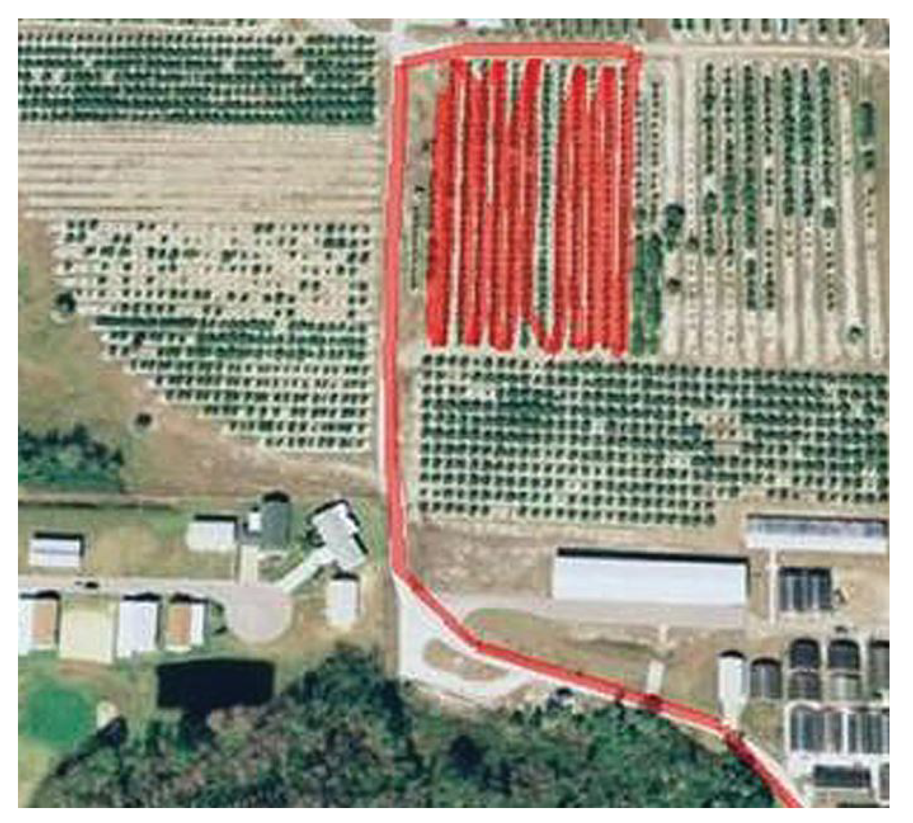
Precision farming benefits from the integration of high-accuracy GPS technology into farm machinery such as combine harvesters, grain carts, tractors, and trucks. Machine data generated by modern agricultural machinery provide crucial information that may be used to obtain valuable insights and forecasts about a farm’s operating plan, present status, and productivity. Additionally, on the basis of predictive analytics, farm operators could make adaptive logistical decisions. Visualisation of GPS data from farm machinery can provide vital information on the operational status and efficiency of a machine. As an example, Figure 1 presents the movement trajectory of a tractor as it worked on a citrus field, and the followed path to and from the field. From the image, it is clear that a row was skipped during the working of the tractor, which can be detrimental to plant growth, especially during spraying and fertiliser application.
A Kalman filter and the Density-Based Spatial Clustering of Applications with Noise (DBSCAN) algorithm were used to detect abnormal activity movement of combine harvesters in [13]. Easting and northing coordinates from GPS logs are iteratively applied to a Kalman filter on the basis of a constant velocity dynamical model. The amount of divergence of the filter estimations from actual data is calculated by using the Kalman filter residual. The Kalman filter residual is a measure of the smoothness of the combine-harvester motion, with a greater residual value indicating a rapid shift in motion. The DBSCAN algorithm method is then applied to the engine load, vehicle speed, and calculated Kalman filter residual, which creates indicative clusters of the combine harvester’s activity. It was feasible to identify clusters for uniform motion on the road, stationary spots, and nonuniform movements on the basis of the findings. Our approach focuses on infield harvest efficiency with special emphasis on local contextual anomalies, which differ from activity detection in this study.
Much effort has gone into developing a variety of anomaly-detection algorithms, which include: distance-based models such as k-nearest neighbours detector (kNN) [14], local outlier factor (LOF) [15]; linear models such as one-class SVM detector [16]; covariance-based models such as minimum covariance determinant (MCD) [3]; ensemble-based models such as locally selective combination of parallel outlier ensembles (LSCP) [17], isolation forest [18], lightweight online detector of anomalies (LODA) [19]; statistical techniques such as histogram-based outlier score (HBOS) [20]; clustering-based models such as clustering-based local outlier factor (CBLOF) [21]; and copula-based models such as the recent copula-based outlier detector (COPOD) [22].
Unsupervised anomaly-detection algorithms automatically identify deviating observations from unlabelled datasets, under some assumptions. Thus, model performance is determined by the different characteristics present in a dataset. Due to this specialisation of the models to different characteristics of observations and resulting in varying detection rates, it is a good idea to integrate the different detection abilities to produce a consensus judgement through the implementation of an ensemble. The combination of these individual abilities is more robust than relying on just one of them [23].
It is also possible that some anomaly-detection algorithms succeed at detecting certain subspaces while others may present poor detection performance [24], although the former’s total accuracy may be lower than that of the latter. This implies that an algorithm can have a domain of expertise in a local domain, yet perform poorly over the entire feature space. It is critical to merge the domains of knowledge of each algorithm in order to reduce overall error [25]. The notion of data locality was first presented by the authors of [26], and it was later enhanced in [27] to perform dynamic classifier selection in local spaces of training points. In comparison to static strategies, such as those that simply vote on the basis of all base classifier outputs, strategies that dynamically pick and combine base classifiers produced better results.
The focus of this research is the identification of anomalies that impact harvest efficiency and those that can be linked to crop state and health during harvest. This study examines anomaly detection in agricultural fields by analysing GPS logs where techniques based on hypothesis testing on the occurrence of an anomalous movement pattern during infield harvesting are utilised. We propose the following contributions:
- 1
- we present a detailed state of the art on anomaly-detection techniques with a focus on smart agriculture;
- 2
- we propose a robust ensemble-based methodology for the detection of anomalies from data streams in smart agriculture context;
- 3
- we apply the proposed technique to a data stream of combine-harvester GPS logs with the aim of identifying anomalies that impact harvest efficiency of farm machinery; and
- 4
- we apply the proposed technique to crop data with the aim of identifying anomalies that reveal the state of the crop during harvest.
This paper is structured as follows. Section 2 presents the temporal datasets corresponding to our two cases of study (the first for harvest GPS logs, the second for the crop-damage dataset) and the preprocessing steps. They correspond to the used materials. It also introduces our anomaly-detection approach, called enhanced LSCP (ELSCP) and the performance indicators that we use. Section 3 shows the experiment results on the two datasets. Section 4 is dedicated to the conclusion.
2. Materials and Methods
In this study, we investigate anomaly detection in two fronts: application to the GPS logs of combine harvesters and detection of crop damage in crop dataset.
2.1. Data Preprocessing and Transformation
2.1.1. Scenario A: Combine Harvester GPS Logs
We used a GPS dataset [28], collected using Nexus 7 tablets on a farm in Colorado USA during the 2019 wheat-harvesting season. A GPS recorder application was kept running for each involved vehicle (combine harvesters, grain carts, and trucks) during harvesting. The combine harvester moved in a straight line at a near constant speed in a normal combine harvester operation (whether harvesting or traveling between fields). The sampling frequency of the data was 1 sample (GPS log) per second. In a typical harvesting scenario, there are more than one harvester working simultaneously in the field. This results in an overlap of the trajectories of the vehicles. A single trajectory is considered as the consolidation of all collected GPS logs belonging to a single combine harvester. For the purpose of this study, we used the movement trajectory of a single combine harvester recorded over a period of three days.
Definition 1.
GPS log: Each GPS log is defined by where:
- is the combine harvester identifier,
- t is the timestamp of the GPS log,
- x is the longitude of the combine at time t,
- y is the latitude of at time t,
- s is the speed of at time t in miles/hour,
- b is the bearing of at time t in degrees
- a is the accuracy of the captured GPS location of at time t
Definition 2.
Trajectory: A raw trajectory consists of time-ordered sequence of n GPS logs of a specific combine harvester such that .
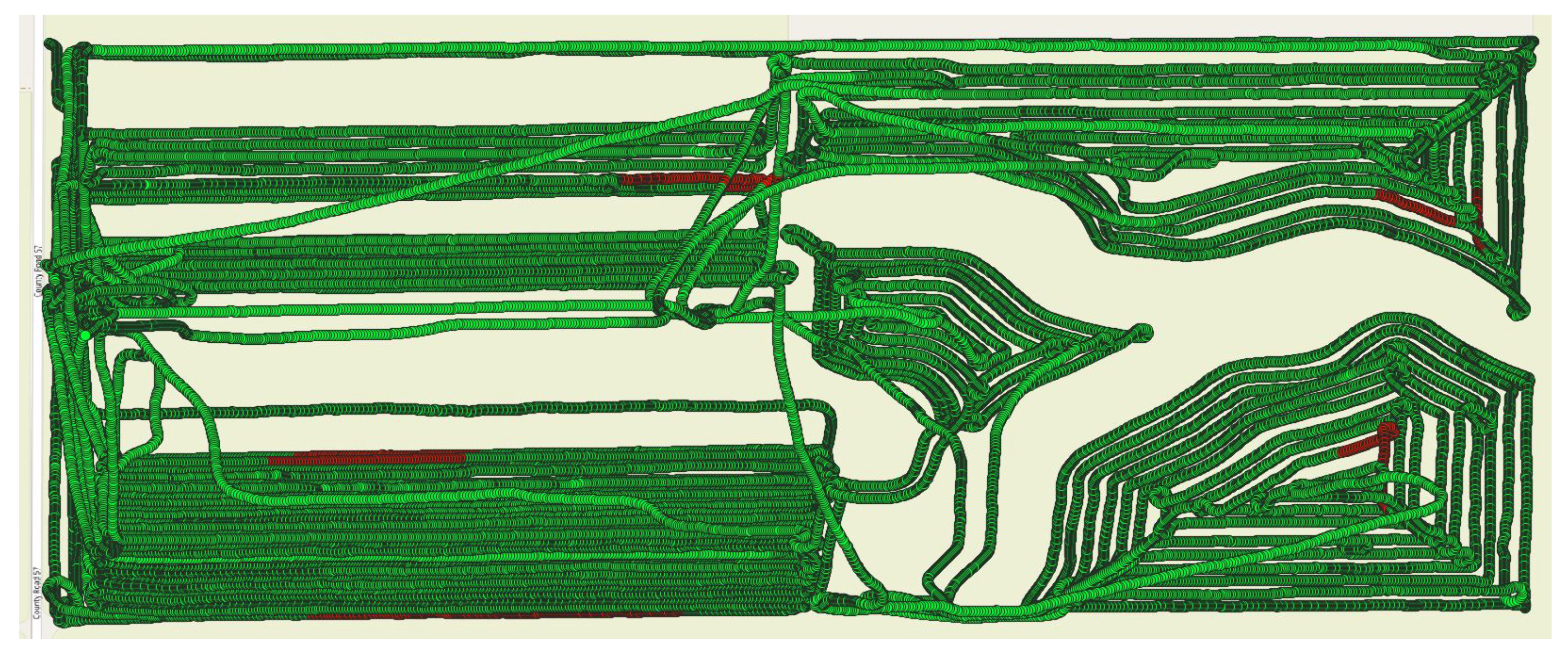
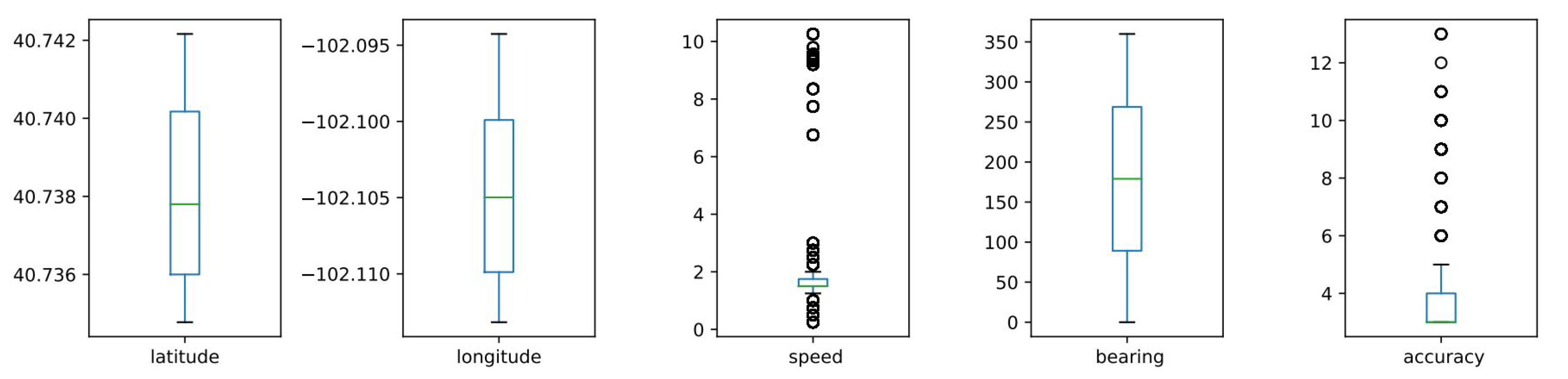
Trajectory mining was performed using Quantum GIS (QGIS), an open-source cross-platform desktop geographic information system application that supports viewing, editing, and visualising geospatial data. The key focus was on data points generated in the field during harvesting; therefore, visualisation and map matching were conducted using QGIS to ensure that GPS points were mapped onto a field. The second step was to extract only those points within a specific field using a bounding box. The extracted data exhibited normal harvesting behaviour with all data points below 4 mph, which is the maximal harvesting speed [29]. The data were further processed by removing all data points with zero speed, since our interest was on GPS points associated to actual grain harvest. To create an evaluation dataset, anomalies were introduced in the original dataset by varying the vehicle speed at specific points along the trajectory, such that, for specific sections of the trajectory, a sequential number of points had their speed increased by a random number between a given range of values above 4 mph. Figure 2 presents the trajectory of a combine harvester after the introduction of anomalies, with normal points in green and anomalies in red. To visualise the effect of the introduced anomalies, outlier analysis was performed using box plots (as shown in Figure 3) that show the presence of outliers in speed and accuracy attributes.
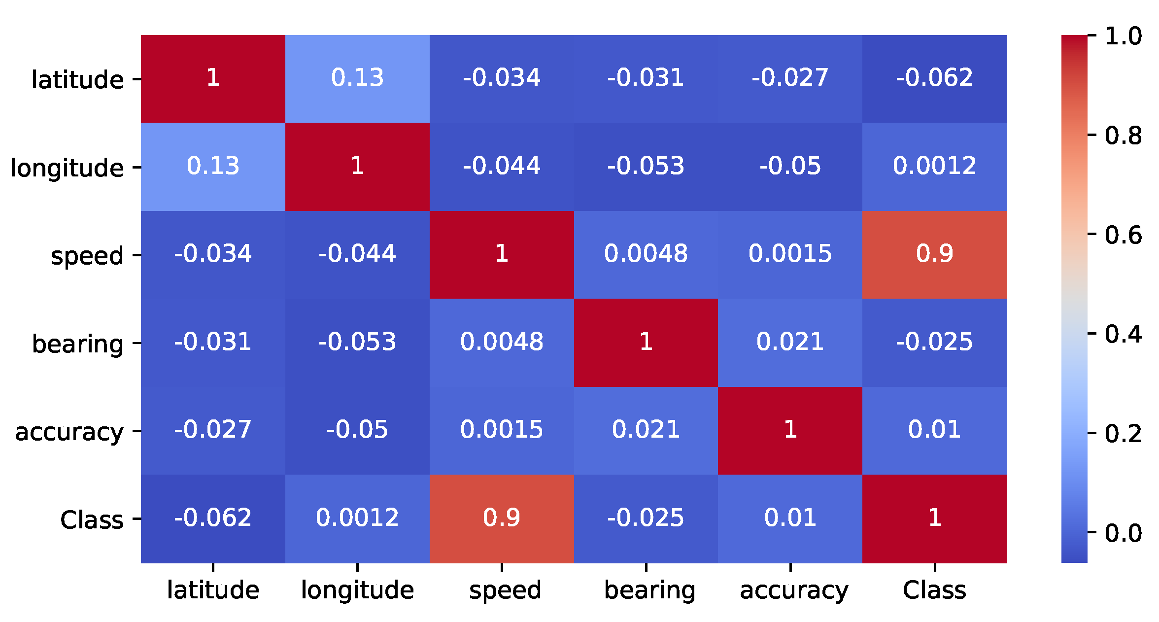
Further data analysis was conducted to establish the existence of any correlation among data attributes through the generation of a correlation heat map (as shown in Figure 4). The map shows a correlation between latitude and longitude, which was expected since these are spatial coordinates. There was also a high positive correlation between speed and class attribute, which is a true representation since introduced anomalies in the data affect the speed attribute.
2.1.2. Scenario B: Crop Dataset
The second scenario considers anomalies in crop data, where the aim was to link the detected anomalies to the state of the crop at the end of the harvest season (i.e., alive or damaged). The crop dataset [30] was collected by various farmers at the end of the harvest season spanning a period of three seasons. To simplify analysis, we assumed that all other factors such as variations in farming technique were controlled. This dataset has 10 variables as summarised in Table 1.
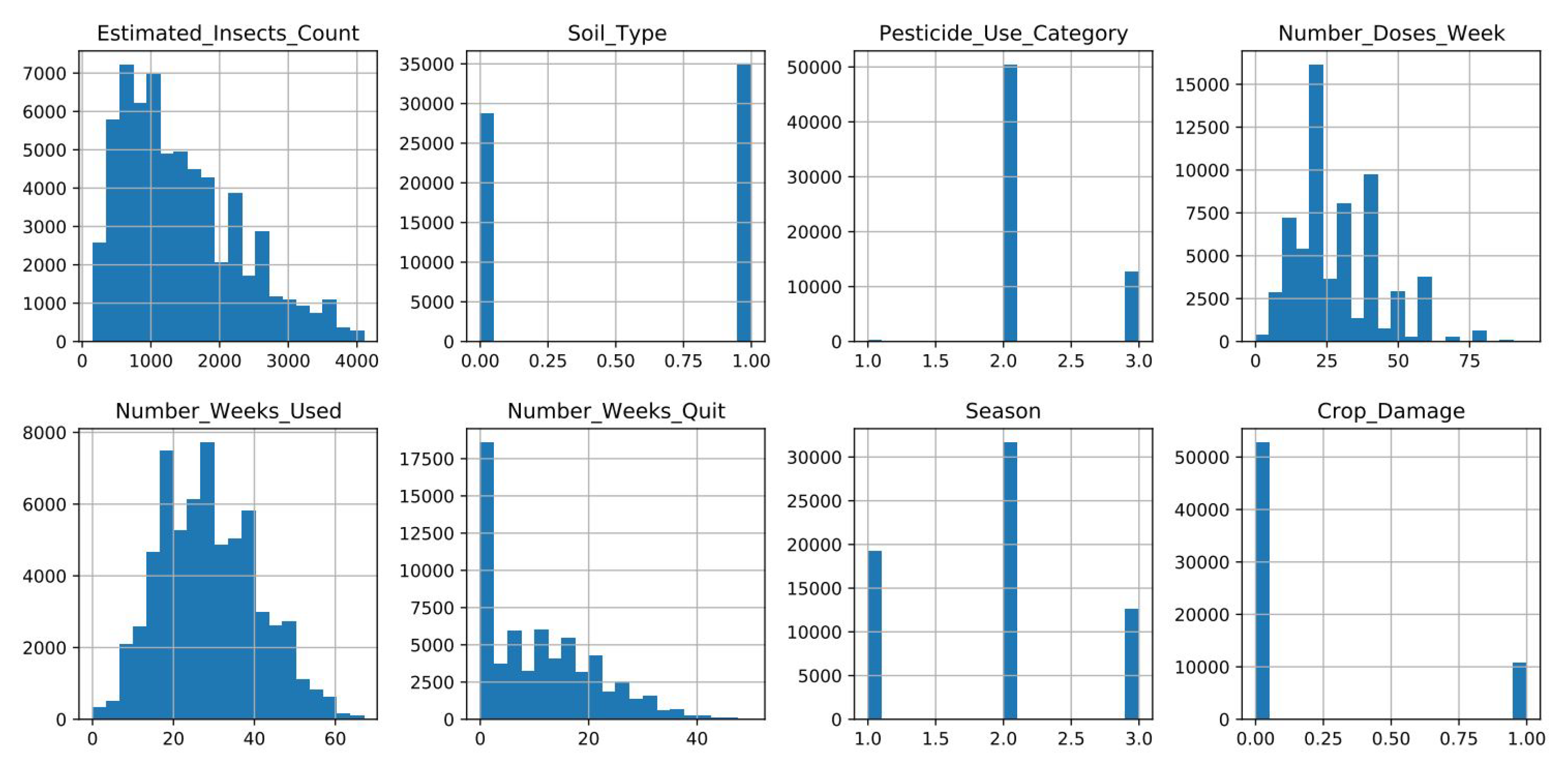
In this study, we consider data for crop type zero (0), which we extracted from the global dataset. The first preprocessing step was to check for missing values in the data, which revealed 6397 missing values in the Number_Weeks_Used variable. The missing data are a result of farmers not recording data for the total number of weeks of pesticide use. Missing values were filled using an iterative imputation technique [31], which performs multivariate imputation by chained equations. In iterative imputation, each feature is modeled as a function of other features. Each feature is imputed one after the other, allowing for previously imputed values to be utilised as part of a model to predict future features.The next step was to check for the distribution of the data per attribute, which is summarised in Figure 5.
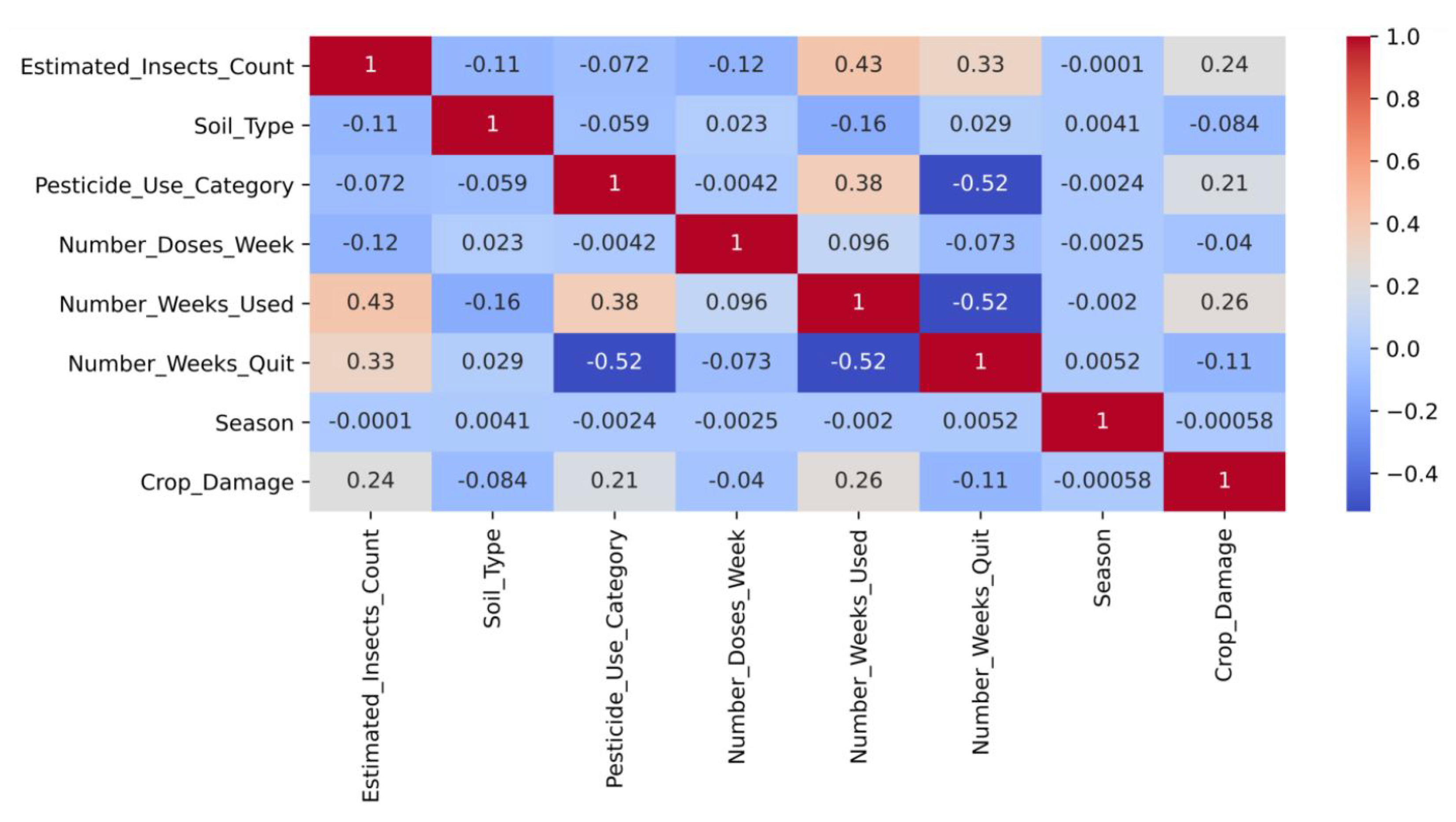
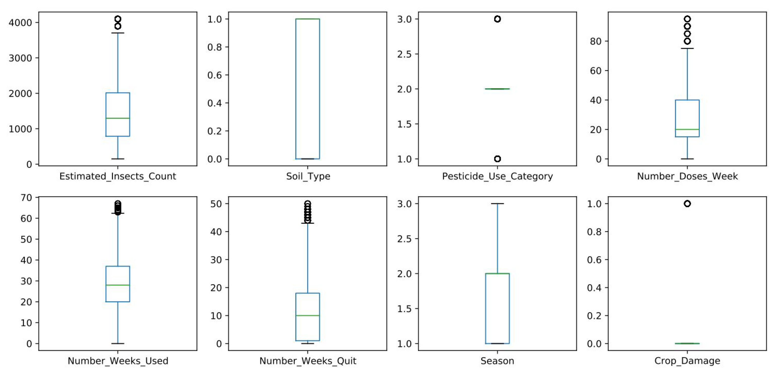
Exploratory data analysis was performed on the crop data, so as to gain a better understanding of the data through the generation of a correlation heat map (as shown in Figure 6). On the basis of the heat map, Estimated_Insects_count, Pesticide_use_category, and Number_weeks_used were positively correlated with crop damage. This indicates that the state of the crop at harvest time was greatly impacted by the presence and number of insects, the type of pesticides used to control these insects, and the duration of exposure to the pesticides. On the other hand, Number_weeks_used was positively correlated with Estimated_Insects_count and Pesticide_use_category. High negative correlation existed, where Number_weeks_Quit was negatively correlated with Pesticide_use_category and Number_weeks_used. Further analysis was also performed to establish the presence of outliers in the dataset. Figure 7 shows that, except for soil type and season, all other attributes had outliers.
2.2. Proposed Approach
The previous section presented the data and preprocessing steps that were performed on them to prepare them for experiments. This section first presents our adaptation and extension of the LSCP approach, which was applied in our experiments on the preprocessed datasets, and, second, the performance indicators that we use.
2.2.1. Enhanced LSCP Algorithm (ELSCP)
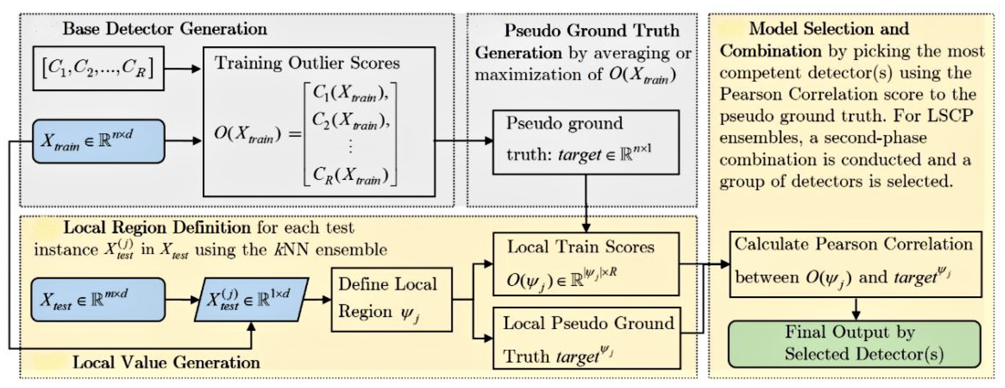
Locally selective combination in parallel outlier ensembles (LSCP) [17] is an unsupervised detector that defines a local region around a test instance by using the consensus of its nearest neighbours in randomly selected feature subspaces. The implementation of LSCP uses an average of maximum strategy where a homogeneous list of base detectors is fitted to the training data; then, pseudo-ground truth is generated for each instance by selecting the maximal outlier score. By training base detectors on the entire dataset and emphasising data locality during detector combination, LSCP examines both global and local data relationships.The process flow of LSCP is summarised in Figure 8.
We propose ELSCP, which is an extension of LSCP with improvements on how the local-region definition is extracted, and competent detectors are selected. To improve local-region definition, we propose to implement local neighbour search by using a ball tree k-nearest neighbours (kNN) algorithm with Harvesine distance metric. We also implemented Kendall correlation in the model selection and combination phase. The procedure for ELSCP starts with a heterogeneous list of base detectors being fitted to the training data. A pseudo-ground truth for each train instance is generated by taking the maximal outlier score from all the base detectors. For each test instance:
- 1
- Using a ball tree nearest neighbour algorithm with Haversine distance metric, the local region is defined to be the set of nearest training points in randomly sampled feature subspaces that occur more frequently using a defined threshold over multiple iterations.
- 2
- Using the local region, a local pseudo-ground truth is defined, and Kendall correlation is calculated between each base detector’s training outlier scores and the pseudo-ground truth.
- 3
- A histogram is built out of Kendall correlation scores, and detectors in the largest bin are selected as competent base detectors for the given test instance.
- 4
- Using the correlation scores, the best detector is selected. The final score for the test instance is computed by using the average of the best detector’s local region scores.
One of the inherent challenges in detection algorithms is how to handle variance and bias, especially in ensemble techniques. According to [32], variance is reduced by integrating heterogeneous base detectors by using techniques such as averaging, maximum of average, and average of maximum. A combination of all base detectors, on the other hand, may contain inaccuracies, resulting in greater bias. As described in Aggarwal’s bias-variance framework, ELSCP combines variance and bias reduction. It improves variance reduction by introducing diversity through the initialisation of numerous base detectors with different hyperparameters. ELSCP also focuses on detector selection based on local competency, which helps identify base detectors with conditionally low model bias.
ELSCP implementation applies three base detectors, HBOS, MCD, and isolation forest (IForest). Histogram-based outlier score (HBOS) [20] is based on the assumption that features are independent, and hence computes outlier scores by creating histograms for each feature. Modelling the precise features of produced histograms and identifying deviations are used to identify anomalies. HBOS does not require data labeling and does not require any training or learning phase. With scoring-based detection, it also provides quick computation, which is important in our context since we process data streams. The isolation forest [18] anomaly-detection algorithm is unsupervised, does not assume the distribution of the data, and does not require labelled data. It also performs well on normal unbiased data with few noise points and is nonparametric [33]. IForest is constructed from a forest of random distinct isolation trees (itrees). IForest properties inform the choice for application in this study because anomalies are rare and different from normal instances; therefore, a tree can be constructed to isolate every instance.
Diagnostics are frequently used in combination with a standard fitting technique to detect outliers. Outliers, on the other hand, can impact these methods, causing the fitted model to miss deviating observations (masking effect) [34]. Robust statistics is a useful technique for discovering these deviating observations since it fits the majority of the data to the fitted model and then identifies data points that differ from the fitted model. In this study, we mitigate the masking effect by implementing minimum covariance determinant (MCD) [35], which is a very reliable estimate for multivariate anomaly identification as one of the base detectors in ELSCP. The determinant of a matrix and Mahalanobis distances are two multivariate feature statistics on which MCD relies. It searches the dataset for observations with the lowest possible determinant in the classical covariance matrix.
2.2.2. Performance Indicators
The balance between false positives and false negatives in anomaly-detection tasks is determined by the application case. False negatives (when no anomaly is discovered while one exists) are usually penalised far more severely than false positives are (a false warning). We use receiver-operating-characteristic (ROC) curves—that is, the true positive rate as a function of the false positive rate—to allow a complete evaluation that is independent of these application-specific trade-offs.
In order to evaluate the performance of the different approaches, we use the area under the curve of the receiver operating characteristic (AUC-ROC) [36] and the area under the curve of precision–recall (AUCPR) [37]. Both indicators are based on the following concepts:
- True positive (TP): true positives are correctly identified anomalies.
- False positive (FP): false positive are incorrectly identified normal data.
- True negative (TN): true negative are correctly identified normal data.
- False negative (FN): false negative are incorrectly rejected anomalies.
True-positive rate (TPR) or recall is
False-positive rate (FPR) is
AUC-ROC receiver operating characteristics are TPR and FPR. The higher the AUC-ROC is, the better the detection is. AUC-ROC is the most popular evaluation measure for unsupervised outlier-detection methods [38].
AUCPR uses precision and recall. Precision is the fraction of retrieved instances that are relevant [39]. Recall or sensitivity is the ability of a model to find all relevant cases within a dataset.
The AUCPR baseline is equivalent to the fraction of positives [40]:
The F1 score (F measure) is the weighted average of precision and recall, and considers both precision (P) and recall (R) rates:
AUCPR is a very robust assessment measure that works well for a wide range of classification tasks. It is particularly useful when dealing with imbalanced data when the minority class is more significant, such as in anomaly detection. Therefore, for the purpose of this study, we evaluate the performance of anomaly-detection algorithms using these indicators.
3. Results
In this section, we present obtained results by experimenting with anomaly-detection techniques on GPS logs and crop data. The algorithms were implemented in Python programming language by using the PyOD framework [41]. Since ELSCP is an ensemble framework, and we used three base detectors in its implementation: HBOS, MCD, and IForest. The reason for using heterogeneous base detectors was to attain unbiased overall detection accuracy with little variance by incorporating the capabilities of different base detectors while carefully combining their outputs to form a robust detector. ELSCP performance ofwas also compared against state-of-the-art anomaly-detection techniques.
3.1. Scenario A: Combine Harvester GPS Data
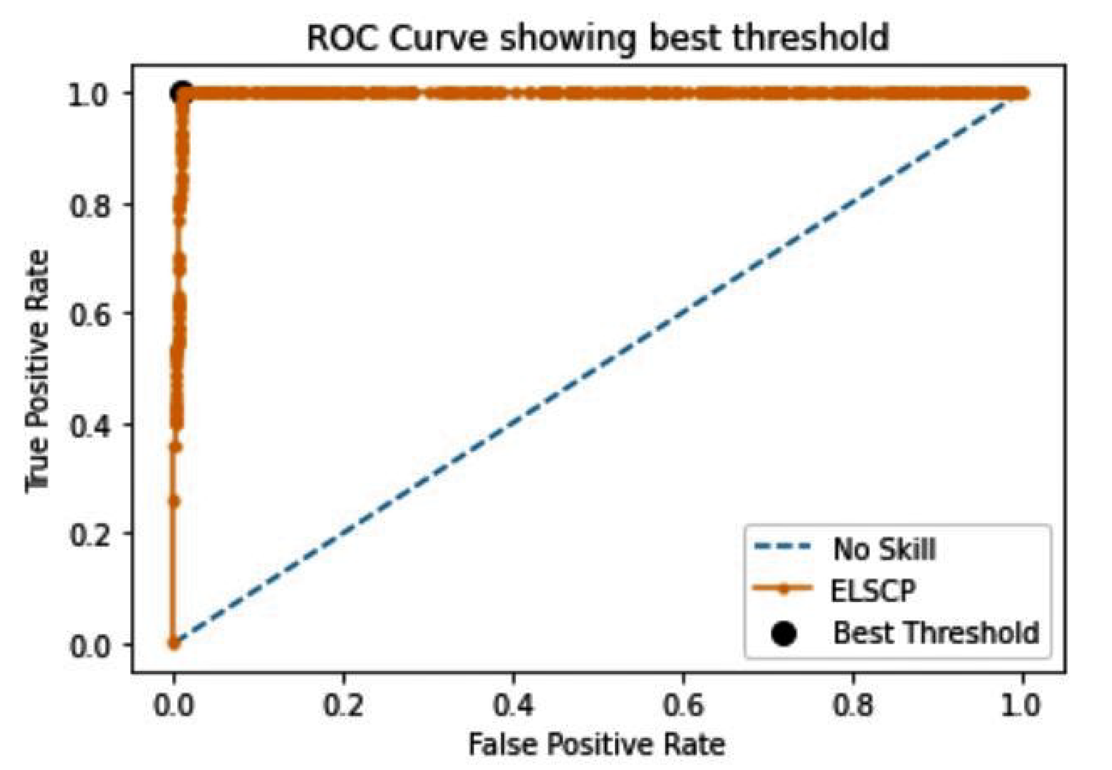
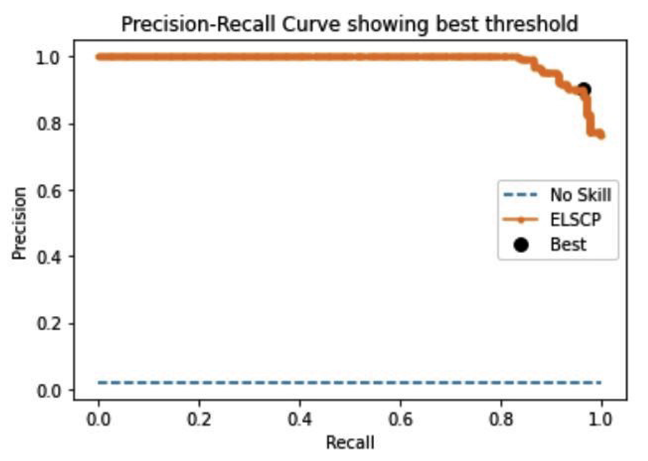
Preprocessed data were then applied to ELSCP, where the aim was to evaluate its performance by looking at the true-positive and false-positive rates by using a ROC curve. AUC-ROC was also computed as an evaluation measure of the model. The baseline AUC-ROC is usually set at a value of 0.5 which suggests that the detector does not discriminate between normal and anomalous data, 0.7 to 0.8 is considered to be acceptable, 0.8 to 0.9 is considered to be excellent, and more than 0.9 is considered to be outstanding [42]. ELSCP was trained with 67% of the data, and prediction performance tested with 33% of the data. ELSCP achieved a global AUC-ROC value of 0.998, which is outstanding performance (as shown in Figure 9). We also evaluated ELCSP performance in terms of precision and recall. The baseline AUCPR for the dataset was 0.0199 (based on a sample size of 51580 with 1026 true-positive anomalies). On the basis of obtained results, ELSCP achieved a global AUCPR of 0.972, which is very good performance (as shown in Figure 10).
In the second set of experiments, we identified the anomaly-detection algorithm that best estimated anomalous instances within GPS logs. We applied the data to ELSCP, baseline LSCP with variants of LOF as base detectors, LODA, COPOD, OCSVM, LOF, and CBLOF. Performance was evaluated by considering each detector’s performance in terms of AUC-ROC, AUCPR, and score. Obtained results from the experiments are summarised in Table 2. According to the results, our approach obtained the best scores with an AUC-ROC that was better than that of the second-best approach COPOD ( vs. ); an AUCPR of , when the best scores of the other approaches (the one of OCSVM) were only . The score reflected the same conclusion ( vs. ). Therefore, our approach was clearly the best, and could help farmers in real time during harvest in detecting potential issues.
3.2. Scenario B: Crop Damage
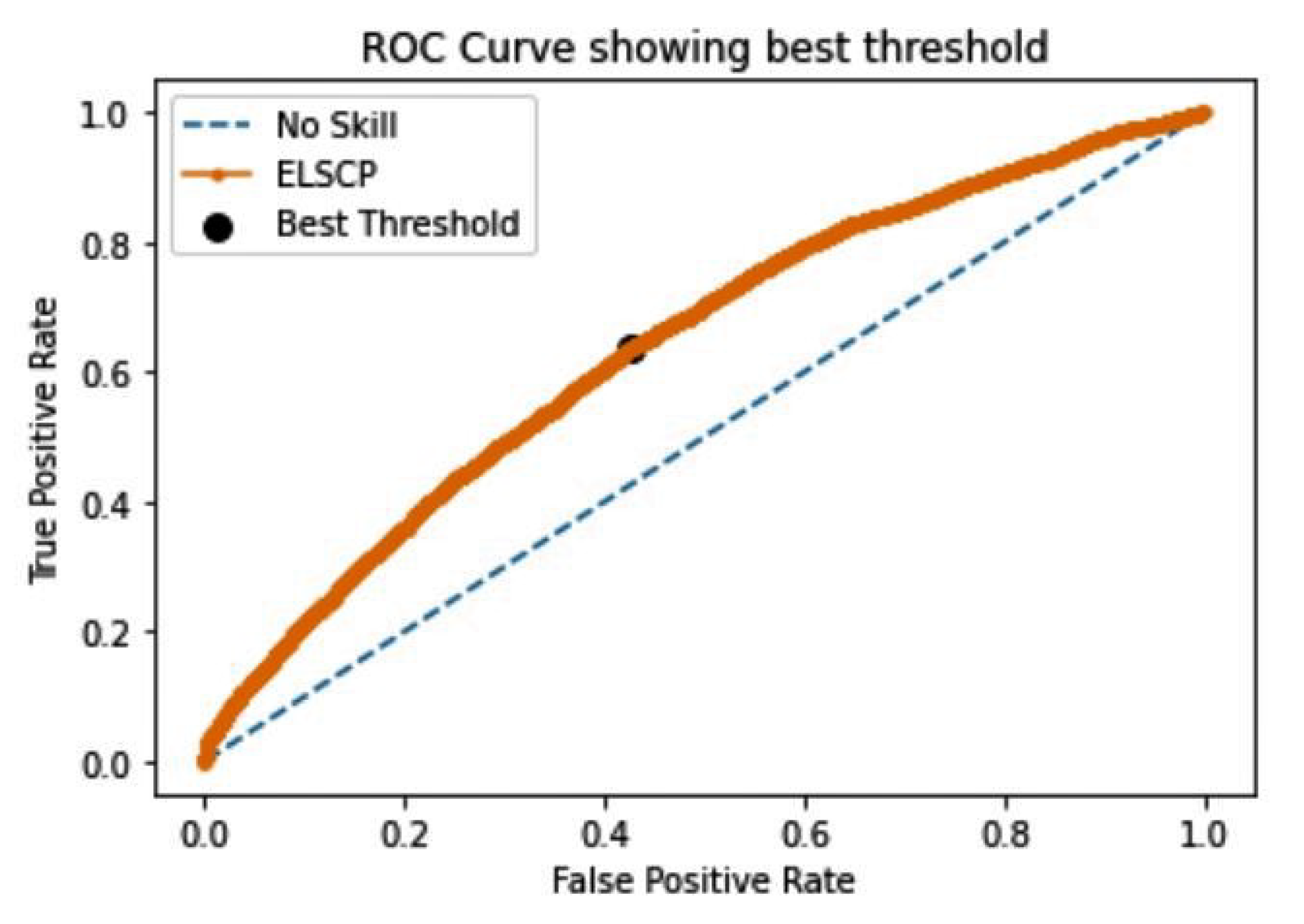
Preprocessed data were then applied to ELSCP where the aim was to evaluate performance by looking at the true-positive and false-positive rates using a ROC curve. AUC-ROC was also computed as an evaluation measure of the model. In the unsupervised outlier-detection setting, it is often problematic to rigorously judge the effectiveness of the algorithms, especially when it outputs an outlier score that is converted into a label on the basis of a threshold. If the threshold selection is too restrictive (to minimise the number of declared outliers), then the algorithm misses true outlier points (false negatives). On the other hand, too many false positives are generated if the algorithm declares too many data points as outliers. To deal with this issue, we performed threshold selection with the aim of the identifying the threshold on the ROC curve that resulted in the best balance between true-positive and false-positive rates for our imbalanced dataset. The Geometric mean (G-mean) was used to compute the optimal threshold, such that the best threshold was the one with the largest G-mean value. The slope of the ROC curve does not affect the performance of an algorithm, since ROC curves are used to make it easier to identify the best threshold from computed probabilities when making a decision on whether an instance is an anomaly or not.
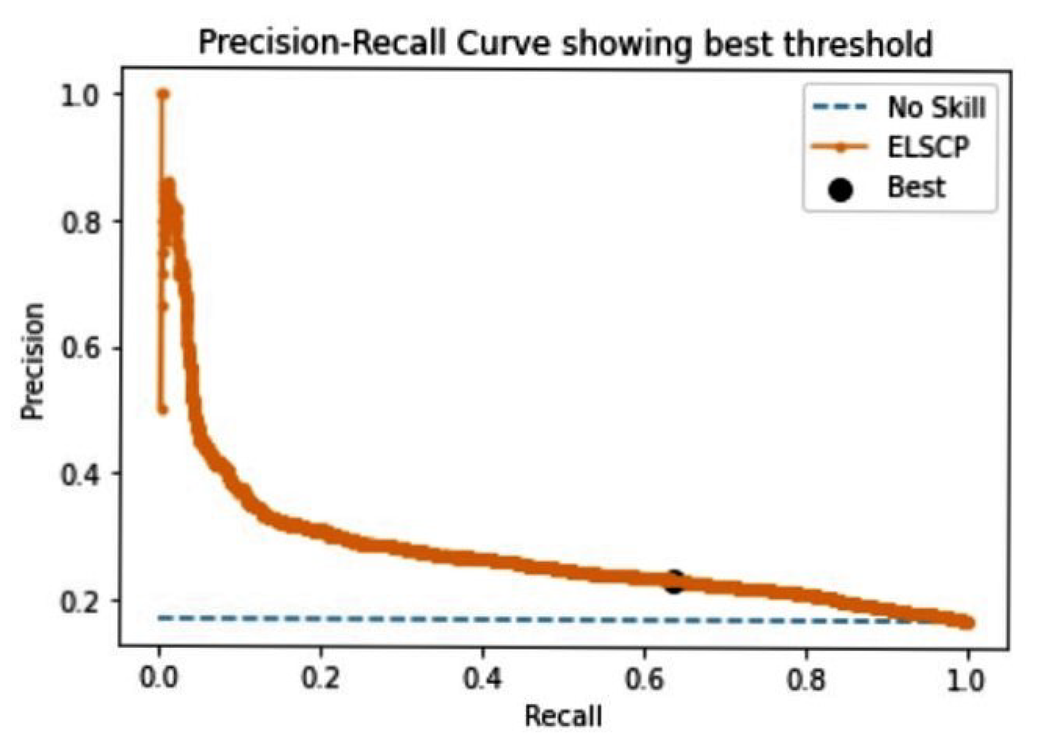
ELSCP was trained with 67% of the data, and prediction performance tested with 33% of the data. The baseline area under the ROC curve is usually set at a value of 0.5, which represents a random guess scenario where the detector does not discriminate between normal and anomalous data. Figure 11 represents the ROC curve showing the best threshold value for ELSCP model. ELSCP achieved 0.641 AUC-ROC, G-mean value of 0.605, and the best threshold ROC value of 0.1404, which shows that it is able to detect anomalies resulting in crop damage. We also evaluated ELCSP performance in terms of precision and recall. The optimal threshold for the precision–recall curve, which focuses on the performance of a model on the positive (minority class/anomalies), was computed by optimising the F measure. The baseline AUCPR for the dataset was 0.17 (based on a sample size of 63589 with 10811 true-positive anomalies). On the basis of obtained results from the precision–recall curve, ELSCP achieved an AUCPR of 0.277 with an score of 0.343 and the best threshold value of 0.1404 (as shown in Figure 12). The obtained AUCPR value is acceptable since it is above the acceptable baseline for the crop dataset.
The second phase of analysis determined if the detected anomalies were linked to the state of the crop being damaged at the end of the harvest season. We extracted all data that had been labelled as anomalies by the model and compared them to the actual ground truth. The model detected 6324 samples as anomalies, of which 1922 (30%) were actual anomalies that were linked to crop damage. In the dataset, the crop state at the end of the harvest could be categorised as alive, damaged due to other causes, or damaged due to pesticides. On the basis of 30% of the actual anomalies, we categorised them according to the cause of damage, where we established that 1641 samples (85.47%) were damage caused by other sources, and 281 samples (14.62%) were damage as a result of pesticide use.
The third phase identified the anomaly-detection algorithm that best estimated the anomalous instances within the crop dataset. We apllied applied the data to ELSCP, baseline LSCP with variants of LOF as base detectors, LODA, COPOD, OCSVM, LOF, and CBLOF. Performance was evaluated by considering each detector’s performance in terms of AUC-ROC, AUCPR, and score. Obtained results from the experiments are summarised in Table 3. According to the results, our approach obtained competitive results where it came second to COPOD with an AUC-ROC margin of ( vs. ) and an AUCPR of vs. of COPOD, which gives a margin of . It achieved the highest score, which was ( vs. ) better than that of the second-best detector, OCSVM. Therefore, our approach is clearly very competitive in this context, and can help farmers in real-time to detect potential issues on crop health.
4. Conclusions
Improving agricultural productivity is critical for increasing farm profitability and fulfilling the world’s fast expanding food demand, which is fuelled by rapid population increase. Precision farming seeks to reduce waste and negative outcomes by precisely focusing agricultural inputs. It has benefited from the integration of high-accuracy GPS technology into farm machinery. Several factors such as water availability, soil fertility, pest protection, timely pesticide application, and nature all contribute to a healthy yield. The precise application of pesticides protects crops from pests, while wrong dosages can result in crop damage or even death. The most versatile and most errorprone anomaly-detection technique is unsupervised anomaly detection. In this case, no data assumptions are made, i.e., the data comprise both normal and anomalous records, and algorithms should be able to distinguish between the two without any prior training. Unsupervised learning is highly preferred for real-life applications, especially in anomaly detection since there are many data without labels in this scenario.
In this study, we performed unsupervised anomaly detection in obtained data streams from movement tracks of combine harvesters during wheat harvest, and data for crop damage recorded by farmers over a period of three harvest seasons. On the basis of our results, deviant combine-harvester behavior could be effectively detected by using machine learning. It was also possible to link anomalies extracted from multivariate analysis of various features to damaged crop state at the end of harvest. Therefore, anomaly detection could be integrated in the decision process of farm operators to improve harvesting efficiency and crop health.
Limitations and Future Work
The first limitation of ELSCP is on the extraction of neighbouring data points that constitute the local region of a test instance using distance metrics applied to KNN Ball Tree algorithm. This approach brings two challenges: (a) it takes much time to determine the nearest neighbours of the test instance; and (b) the performance in a multidimensional space may be affected, especially when many features or attributes are irrelevant. To mitigate this challenge, local-region definition can be solved by clustering [43], the use of fast approximate methods [44] or by prototyping [45], which can significantly reduce the required time to set up the local domain because not all data points are required by these techniques. The second limitation is on the generation of the pseudo-ground truth, where we applied a simple maximisation technique. This could be improved by considering exact strategies, for instance, with the active pruning of base detectors [46].
Our future work will focus on addressing model calibration and hyperparameter tuning to improve on outlier scoring since a false negative in smart agriculture can induce uncomfortable issues in crop production and farm efficiency. The configuration of local subspaces can also be improved to decrease the amount of time spent locating a test instance’s nearest neighbours by replacing the kNN search strategy with a clustering technique. We also propose to develop the methodology into a tool that can be used by farmers and experts for the real-time detection and analysis of farming data streams.
Author Contributions
Conceptualisation, J.C.M., S.C., C.d.R., H.F. and J.M.W.; methodology, J.C.M., S.C., C.d.R., H.F.; software, J.C.M.; validation, J.C.M., C.d.R. and H.F.; formal analysis, J.C.M.; investigation, J.C.M.; resources, J.C.M.; data curation, J.C.M.; writing—original draft preparation, J.C.M.; writing—review and editing, S.C., C.d.R., H.F. and J.M.W.; visualisation, J.C.M.; supervision, S.C., C.d.R., H.F. and J.M.W.; project administration, S.C., H.F. and J.M.W.; funding acquisition, J.C.M., S.C., C.d.R., H.F. and J.M.W. All authors have read and agreed to the published version of the manuscript.
Funding
This research was partially funded by the French Embassy in Kenya.
Data Availability Statement
Publicly available datasets were analysed in this study. The first dataset (Combine Kart Truck GPS Data Archive) is openly available at https://purr.purdue.edu/publications/3083/2 (accessed on 5 July 2021), reference number [28]. The second dataset (AV JanataHack: Machine Learning in Agriculture) is openly available at https://www.kaggle.com/shravankoninti/av-janatahack-machine-learning-in-agriculture (accessed on 5 July 2021).
Conflicts of Interest
The authors declare no conflict of interest.
Abbreviations
The following abbreviations are used in this manuscript:
| ANNs | Artificial neural networks |
| AUC-ROC | Area under the curve of the receiver operating characteristic |
| AUCPR | Area Under the Curve of Precision-Recall |
| ARIMA | Autoregressive integrated moving average model |
| CBLOF | Clustering-based local outlier factor |
| COPOD | Copula-based outlier detector |
| DBSCAN | Density-based spatial clustering of applications with noise |
| ELSCP | Enhanced locally selective combination in parallel outlier ensembles |
| FP | False positive |
| FPR | False-positive rate |
| FN | False negative |
| GPS | Global positioning system |
| GPU | Graphics processing unit |
| HBOS | Histogram-based outlier score |
| IQR | Interquartile range |
| kNN | k-nearest neighbours detector |
| LOF | Local outlier factor |
| LODA | Lightweight online detector of anomalies |
| LSTM | Long short-term memory |
| LSCP | Locally selective combination in parallel outlier ensembles |
| MCD | Minimum covariance determinant |
| OCSVM | One-class support vector machines |
| P | Precision |
| PyOD | Python outlier detection |
| QGIS | Quantum geographic information system |
| R | Recall |
| SAR | Synthetic aperture radar |
| SVM | Support vector machine |
| TP | True positive |
| TPR | True positive rate |
| TN | True negative |
References
- Allahyari, M.S.; Damalas, C.A.; Ebadattalab, M. Farmers’ technical knowledge about integrated pest management (IPM) in olive production. Agriculture 2017, 7, 101. [Google Scholar] [CrossRef] [Green Version]
- Fargnoli, M.; Lombardi, M.; Puri, D. Applying hierarchical task analysis to depict human safety errors during pesticide use in vineyard cultivation. Agriculture 2019, 9, 158. [Google Scholar] [CrossRef] [Green Version]
- Chandola, V.; Banerjee, A.; Kumar, V. Anomaly detection: A survey. ACM Comput. Surv. (CSUR) 2009, 41, 1–58. [Google Scholar] [CrossRef]
- Ou, C.H.; Chen, Y.A.; Huang, T.W.; Huang, N.F. Design and Implementation of Anomaly Condition Detection in Agricultural IoT Platform System. In Proceedings of the 2020 International Conference on Information Networking (ICOIN), Barcelona, Spain, 7–10 January 2020; pp. 184–189. [Google Scholar]
- Christiansen, P.; Nielsen, L.N.; Steen, K.A.; Jørgensen, R.N.; Karstoft, H. DeepAnomaly: Combining background subtraction and deep learning for detecting obstacles and anomalies in an agricultural field. Sensors 2016, 16, 1904. [Google Scholar] [CrossRef] [Green Version]
- Xu, J.; Guga, S.; Rong, G.; Riao, D.; Liu, X.; Li, K.; Zhang, J. Estimation of Frost Hazard for Tea Tree in Zhejiang Province Based on Machine Learning. Agriculture 2021, 11, 607. [Google Scholar] [CrossRef]
- Abdallah, M.; Lee, W.J.; Raghunathan, N.; Mousoulis, C.; Sutherland, J.W.; Bagchi, S. Anomaly Detection through Transfer Learning in Agriculture and Manufacturing IoT Systems. arXiv 2021, arXiv:2102.05814. [Google Scholar]
- Mouret, F.; Albughdadi, M.; Duthoit, S.; Kouamé, D.; Rieu, G.; Tourneret, J.Y. Outlier detection at the parcel-level in wheat and rapeseed crops using multispectral and SAR time series. Remote Sens. 2021, 13, 956. [Google Scholar] [CrossRef]
- Blackmore, S. The interpretation of trends from multiple yield maps. Comput. Electron. Agric. 2000, 26, 37–51. [Google Scholar] [CrossRef]
- Matheron, G. Principles of geostatistics. Econ. Geol. 1963, 58, 1246–1266. [Google Scholar] [CrossRef]
- Blackmore, S.; Godwin, R.J.; Fountas, S. The analysis of spatial and temporal trends in yield map data over six years. Biosyst. Eng. 2003, 84, 455–466. [Google Scholar] [CrossRef]
- Ehsani, R. Increasing field efficiency of farm machinery using GPS. EDIS. 2010, 2010. Available online: https://journals.flvc.org/edis/article/view/118721 (accessed on 23 September 2021).
- Wang, Y.; Balmos, A.; Krogmeier, J.; Buckmaster, D. Data-Driven Agricultural Machinery Activity Anomaly Detection and Classification. In Proceedings of the 14th International Conference on Precision Agriculture, Montreal, Quebec, Canada, 24–27 June 2018. [Google Scholar]
- Ramaswamy, S.; Rastogi, R.; Shim, K. Efficient algorithms for mining outliers from large data sets. In Proceedings of the 2000 ACM SIGMOD International Conference on Management of Data, Dallas, TX, USA, 15–18 May 2000; pp. 427–438. [Google Scholar]
- Breunig, M.M.; Kriegel, H.P.; Ng, R.T.; Sander, J. LOF: identifying density-based local outliers. In Proceedings of the 2000 ACM SIGMOD International Conference on Management of Data, Dallas, TX, USA, 15–18 May 2000; pp. 93–104. [Google Scholar]
- Schölkopf, B.; Platt, J.C.; Shawe-Taylor, J.; Smola, A.J.; Williamson, R.C. Estimating the support of a high-dimensional distribution. Neural Comput. 2001, 13, 1443–1471. [Google Scholar] [CrossRef] [PubMed]
- Zhao, Y.; Nasrullah, Z.; Hryniewicki, M.K.; Li, Z. LSCP: Locally selective combination in parallel outlier ensembles. In Proceedings of the 2019 SIAM International Conference on Data Mining, SIAM, Calgary, Alberta, Canada, 2–4 May 2019; pp. 585–593. [Google Scholar]
- Liu, F.T.; Ting, K.M.; Zhou, Z.H. Isolation forest. In Proceedings of the 2008 Eighth IEEE International Conference on Data Mining, Pisa, Italy, 15–19 December 2008; pp. 413–422. [Google Scholar]
- Pevnỳ, T. Loda: Lightweight on-line detector of anomalies. Mach. Learn. 2016, 102, 275–304. [Google Scholar] [CrossRef] [Green Version]
- Goldstein, M.; Dengel, A. Histogram-based outlier score (hbos): A fast unsupervised anomaly detection algorithm. In KI-2012: Poster and Demo Track; 2012. Available online: https://www.goldiges.de/publications/HBOS-KI-2012.pdf (accessed on 23 September 2021).
- He, Z.; Xu, X.; Deng, S. Discovering cluster-based local outliers. Pattern Recognit. Lett. 2003, 24, 1641–1650. [Google Scholar] [CrossRef]
- Li, Z.; Zhao, Y.; Botta, N.; Ionescu, C.; Hu, X. COPOD: copula-based outlier detection. In Proceedings of the 2020 IEEE International Conference on Data Mining (ICDM), Sorrento, Italy, 17–20 November 2020; pp. 1118–1123. [Google Scholar]
- Zimek, A.; Campello, R.J.; Sander, J. Ensembles for unsupervised outlier detection: challenges and research questions a position paper. ACM Sigkdd Explor. Newsl. 2014, 15, 11–22. [Google Scholar] [CrossRef]
- Britto Jr, A.S.; Sabourin, R.; Oliveira, L.E. Dynamic selection of classifiers—A comprehensive review. Pattern Recognit. 2014, 47, 3665–3680. [Google Scholar] [CrossRef]
- Polikar, R. Ensemble based systems in decision making. IEEE Circuits Syst. Mag. 2006, 6, 21–45. [Google Scholar] [CrossRef]
- Ho, T.K.; Hull, J.J.; Srihari, S.N. Decision combination in multiple classifier systems. IEEE Trans. Pattern Anal. Mach. Intell. 1994, 16, 66–75. [Google Scholar]
- Woods, K.; Kegelmeyer, W.P.; Bowyer, K. Combination of multiple classifiers using local accuracy estimates. IEEE Trans. Pattern Anal. Mach. Intell. 1997, 19, 405–410. [Google Scholar] [CrossRef]
- Zhang, Y.; Krogmeier, J. Combine Kart Truck GPS Data Archive. Purdue University Research Repository. 2020. Available online: https://purr.purdue.edu/publications/3083/2 (accessed on 23 September 2021). [CrossRef]
- Zhang, Y.; Balmos, A.; Krogmeier, J.V.; Buckmaster, D. Working zone identification for specialized micro transportation systems using GPS tracks. In Proceedings of the 2015 IEEE 18th International Conference on Intelligent Transportation Systems, Canary Islands, Spain, 15–18 September 2015; pp. 1779–1784. [Google Scholar]
- Koninti, S.K. AV JanataHack: Machine Learning in Agriculture; Analytics Vidhya, 2020. Available online: https://datahack.analyticsvidhya.com/contest/janatahack-machine-learning-in-agriculture/#DiscussTab (accessed on 23 September 2021).
- Van Buuren, S.; Groothuis-Oudshoorn, K. mice: Multivariate imputation by chained equations in R. J. Stat. Softw. 2011, 45, 1–67. [Google Scholar] [CrossRef] [Green Version]
- Aggarwal, C.C.; Sathe, S. Theoretical foundations and algorithms for outlier ensembles. ACM Sigkdd Explor. Newsl. 2015, 17, 24–47. [Google Scholar] [CrossRef]
- Aggarwal, C.C. Outlier analysis. In Data Mining; Springer: Berlin, Germany, 2015; pp. 237–263. [Google Scholar]
- Rousseeuw, P.J.; Hubert, M. Anomaly detection by robust statistics. Wiley Interdiscip. Rev. Data Min. Knowl. Discov. 2018, 8, e1236. [Google Scholar] [CrossRef] [Green Version]
- Rousseeuw, P.J.; Driessen, K.V. A fast algorithm for the minimum covariance determinant estimator. Technometrics 1999, 41, 212–223. [Google Scholar] [CrossRef]
- Hanley, J.A.; McNeil, B.J. The meaning and use of the area under a receiver operating characteristic (ROC) curve. Radiology 1982, 143, 29–36. [Google Scholar] [CrossRef] [Green Version]
- Boyd, K.; Eng, K.H.; Page, C.D. Area under the precision-recall curve: Point estimates and confidence intervals. In Joint European Conference on Machine Learning and Knowledge Discovery in Databases; Springer: Berlin, Germany, 2013; pp. 451–466. [Google Scholar]
- Campos, G.O.; Zimek, A.; Sander, J.; Campello, R.J.; Micenková, B.; Schubert, E.; Assent, I.; Houle, M.E. On the evaluation of unsupervised outlier detection: measures, datasets, and an empirical study. Data Min. Knowl. Discov. 2016, 30, 891–927. [Google Scholar] [CrossRef]
- Fawcett, T. An introduction to ROC analysis. Pattern Recognit. Lett. 2006, 27, 861–874. [Google Scholar] [CrossRef]
- Saito, T.; Rehmsmeier, M. The precision-recall plot is more informative than the ROC plot when evaluating binary classifiers on imbalanced datasets. PLoS ONE 2015, 10, e0118432. [Google Scholar] [CrossRef] [PubMed] [Green Version]
- Zhao, Y.; Nasrullah, Z.; Li, Z. PyOD: A Python Toolbox for Scalable Outlier Detection. J. Mach. Learn. Res. 2019, 20, 1–7. [Google Scholar]
- Mandrekar, J.N. Receiver operating characteristic curve in diagnostic test assessment. J. Thorac. Oncol. 2010, 5, 1315–1316. [Google Scholar] [CrossRef] [Green Version]
- Wang, B.; Mao, Z. Outlier detection based on a dynamic ensemble model: Applied to process monitoring. Inf. Fusion 2019, 51, 244–258. [Google Scholar] [CrossRef]
- Hajebi, K.; Abbasi-Yadkori, Y.; Shahbazi, H.; Zhang, H. Fast approximate nearest-neighbor search with k-nearest neighbor graph. In Proceedings of the Twenty-Second International Joint Conference on Artificial Intelligence, Centre, Convencions Internacional Barcelona, 19–22 July 2011. [Google Scholar]
- Cruz, R.M.; Sabourin, R.; Cavalcanti, G.D. Dynamic classifier selection: Recent advances and perspectives. Inf. Fusion 2018, 41, 195–216. [Google Scholar] [CrossRef]
- Rayana, S.; Akoglu, L. Less is more: Building selective anomaly ensembles. ACM Trans. Knowl. Discov. Data (TKDD) 2016, 10, 1–33. [Google Scholar] [CrossRef]
Figure 1.
Movement trajectory of a tractor in a citrus grove [12].
Figure 1.
Movement trajectory of a tractor in a citrus grove [12].

Figure 2.
Field of interest: trajectory of a combine harvester showing normal points in green and anomalies in red.
Figure 2.
Field of interest: trajectory of a combine harvester showing normal points in green and anomalies in red.

Figure 3.
Attribute-based box plots showing presence of outliers in combine harvester GPS logs.

Figure 4.
Heat map showing correlation between attributes of combine harvester GPS log dataset.

Figure 5.
Histograms showing data distribution per attribute in crop dataset.

Figure 6.
Heat map showing correlation between attributes of the crop dataset.

Figure 7.
Attribute-based box plots showing presence of outliers in the crop dataset.

Figure 8.
LSCP flowchart. Steps requiring recomputation highlighted in yellow; cached steps in grey [17].
Figure 8.
LSCP flowchart. Steps requiring recomputation highlighted in yellow; cached steps in grey [17].

Figure 9.
ELSCP ROC curve performance evaluation for combine-harvester GPS dataset.

Figure 10.
ELSCP precision–recall performance evaluation combine-harvester GPS dataset.

Figure 11.
ELSCP ROC curve indicating best prediction threshold for the crop dataset.

Figure 12.
ELSCP precision–recall curve indicating best prediction threshold for the crop dataset.


Table 1.
Crop Data Description.
| Column Name | Description |
|---|---|
| Id | UniqueID |
| Estimated_Insects_Count | Estimated insects count per square meter |
| Crop_Type | Category of Crop(0,1) |
| Soil_Type | Category of Soil (0,1) |
| Pesticide_Use_Category | Type of pesticides used (1, never; 2, previously used; 3, currently using) |
| Number_Doses_Week | Number of doses per week |
| Number_Weeks_Used | Number of weeks used |
| Number_Weeks_Quit | Number of weeks pesticide not used |
| Season | Season Category (1,2,3) |
| Crop_Damage | Crop damage category (0 = alive, 1 = damage due to other causes, 2 = damage due to pesticides) |
Table 2.
Performance comparison of various detectors on combine harvester GPS logs.
| Model | AUC-ROC | AUCPR | F1 Score |
|---|---|---|---|
| ELSCP | 0.998 | 0.972 | 0.921 |
| OCSVM | 0.897 | 0.385 | 0.167 |
| LODA | 0.913 | 0.215 | 0.078 |
| COPOD | 0.934 | 0.173 | 0.228 |
| CBLOF | 0.756 | 0.038 | 0.014 |
| LSCP | 0.533 | 0.022 | 0.032 |
Table 3.
Performance comparison of various detectors on drop dataset.
| Model | AUC-ROC | AUCPR | F1 Score |
|---|---|---|---|
| ELSCP | 0.641 | 0.277 | 0.343 |
| OCSVM | 0.595 | 0.253 | 0.291 |
| LODA | 0.580 | 0.200 | 0.122 |
| COPOD | 0.675 | 0.297 | 0.282 |
| CBLOF | 0.636 | 0.226 | 0.212 |
| LSCP | 0.452 | 0.169 | 0.135 |
Publisher’s Note: MDPI stays neutral with regard to jurisdictional claims in published maps and institutional affiliations. |
© 2021 by the authors. Licensee MDPI, Basel, Switzerland. This article is an open access article distributed under the terms and conditions of the Creative Commons Attribution (CC BY) license (https://creativecommons.org/licenses/by/4.0/).
Share and Cite
MDPI and ACS Style
Moso, J.C.; Cormier, S.; de Runz, C.; Fouchal, H.; Wandeto, J.M. Anomaly Detection on Data Streams for Smart Agriculture. Agriculture 2021, 11, 1083. https://doi.org/10.3390/agriculture11111083
AMA Style
Moso JC, Cormier S, de Runz C, Fouchal H, Wandeto JM. Anomaly Detection on Data Streams for Smart Agriculture. Agriculture. 2021; 11(11):1083. https://doi.org/10.3390/agriculture11111083
Chicago/Turabian StyleMoso, Juliet Chebet, Stéphane Cormier, Cyril de Runz, Hacène Fouchal, and John Mwangi Wandeto. 2021. "Anomaly Detection on Data Streams for Smart Agriculture" Agriculture 11, no. 11: 1083. https://doi.org/10.3390/agriculture11111083
Note that from the first issue of 2016, this journal uses article numbers instead of page numbers. See further details here.