A Combined Nonstationary Kriging and Support Vector Machine Method for Stochastic Eigenvalue Analysis of Brake Systems

Abstract

This paper presents a new metamodel approach based on nonstationary kriging and a support vector machine to efficiently predict the stochastic eigenvalue of brake systems. One of the difficulties in the mode-coupling instability induced by friction is that stochastic eigenvalues represent heterogeneous behavior due to the bifurcation phenomenon. Therefore, the stationarity assumption in kriging, where the response is correlated over the entire random input space, may not remain valid. In this paper, to address this issue, Gibb’s nonstationary kernel with step-wise hyperparameters was adopted to reflect the heterogeneity of the stochastic eigenvalues. In predicting the response for unsampled input, the support vector machine-based classification is utilized. To validate the performance, a simplified finite element model of the brake system is considered. Under various types of uncertainties, including different friction coefficients and material properties, stochastic eigenvalue problems are investigated. Through numerical studies, it is seen that the proposed method improves accuracy and robustness compared to conventional stationary kriging.

1. Introduction

Brake systems subjected to friction-induced vibration are widely used in many industrial applications such as the automobile, aircraft, and railway fields [1]. One of the important vibration characteristics caused by friction is instability mechanisms, which can be classified into four categories: Variable friction coefficient, stick-slip, sprag-slip, and mode-coupling [2]. Among these various types of instabilities, mode-coupling is considered one of the most crucial mechanisms [3]; one phenomenon that is observed when this mechanism occurs is that the real parts of the eigenvalues bifurcate, while the associated imaginary parts are merged. Since the stability of the system can be determined from the eigenvalues, many studies have been conducted to investigate the phenomenon through complex eigenvalue analyses (CEA) [4,5,6].

In carrying out CEA, the computational model is usually considered as deterministic, and the fixed friction coefficient is applied. However, the friction coefficient is known to have strong dispersion characteristics depending on the operation conditions [7], and should be modeled as a random parameter. In addition, most physical systems are subject to uncertainties concerning the input parameters, such as the material properties and geometry, and the contact conditions. Therefore, it is necessary to consider uncertainties to ensure that a robust analysis of brake systems can be made.

The stochastic eigenvalue problem is an extension of the deterministic problem to study response variability under parametric input uncertainties. Several methods have been proposed, such as Monte Carlo simulation (MCS), a sensitivity-based approach, polynomial chaos expansion (PCE), and kriging (Gaussian process). MCS [8] is a sampling-based technique which is considered the most robust method for uncertainty quantifications. However, since a large number of samples must be drawn to obtain sufficient accuracy, the computational cost becomes prohibitive. The sensitivity-based method [9] is a low-order Taylor expansion method that approximates the solution near the input parameters. Although this method is computationally efficient, the obtained solution will be inaccurate under large parameter variabilities.

PCE and kriging are metamodel (surrogate model) -based techniques that replace the original model with an easy-to-evaluate function. PCE [10], also known as a spectral approach, is a regression-based methods that approximates the model by multivariate polynomials. Kriging [11] is an interpolation-based approach in which the model is assumed to be a realization of a Gaussian process. Since metamodel-based methods can be applied to various levels of uncertainty, numerous studies have utilized them to solve stochastic eigenvalue problems in brake systems [12,13,14,15].

However, despite previous studies, it remains challenging to apply PCE and kriging to brake systems with the mode-coupling phenomenon. Since eigenvalues exhibit nonsmooth behavior around the bifurcation point, PCE is not adequate for capturing local solution accuracy. Several studies have tackled this issue by applying multi-element PCE [16], a wavelet basis [17]. Although kriging interpolates each sample and reflects the local characteristics, to the authors’ knowledge, previous studies have all been based on the stationarity assumption, which means that the smoothness of response is entirely correlated throughout the random input space. Therefore, for mode-coupling problems where the stationarity assumption is violated, the results are highly sensitive to the samples, and accuracy and robustness will be compromised.

In this paper, to address this issue, we propose a new combined nonstationary kriging and support vector machine method for stochastic analyses of the brake systems. The main difference from conventional stationary kriging is that the proposed algorithm utilizes a nonstationary kernel to reflect the bifurcation characteristics of the eigenvalues. In predicting the response for unsampled input, one difficulty arising from the nonstationary kernel is to construct a correlation vector. To resolve this problem, support vector machine-based classification is applied.

The rest of this paper is organized as follows. In Section 2, we present the formulation of the stochastic complex eigenvalue problem. Section 3 describes our proposed algorithm. In Section 4, the proposed method is verified through numerical studies. Finally, we provide concluding remarks.

2. Stochastic Complex Eigenvalue Analysis of Brake System

2.1. Finite Element Model of the Brake System

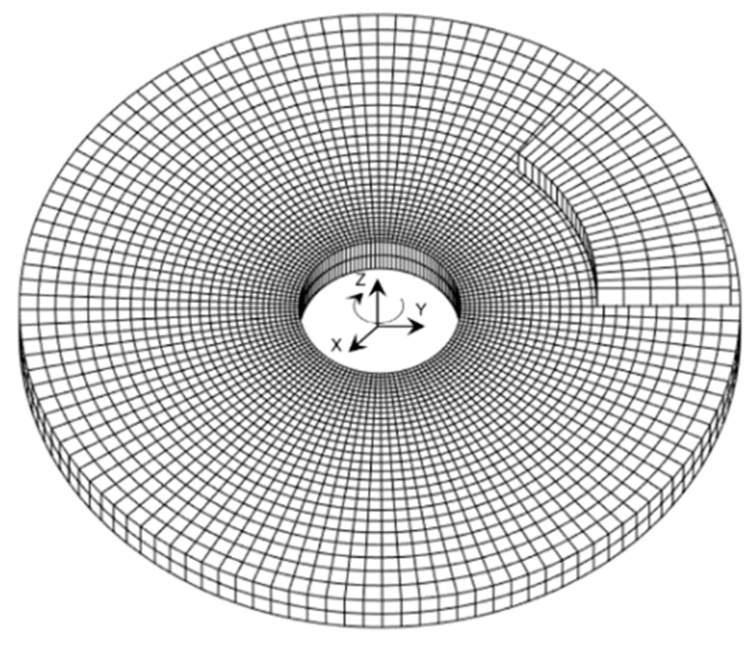
The finite element model of the simplified brake system used in this study is illustrated in Figure 1. This model is taken from [15] and the parameters are listed in

Table 1. Model properties of the simplified brake system.

Parameters	Disc	Pad
Young’s modulus $E$ (N/m2)	125 × 109	2 × 109
Poisson ratio $\nu$	0.3	0.1
Density $\rho$ (kg/m3)	7200	2500
Inner radius (m)	0.034	0.091
Outer radius (m)	0.151	0.147
Thickness (m)	0.019	0.0128

.

To discretize the given geometry, low order hexahedral elements are applied, and a total of 10,692 nodes and 6820 elements are used. The total DOF of the given model is 32,076. When applying the boundary conditions, the disc’s inner surface and in-plane of the pad are fixed.

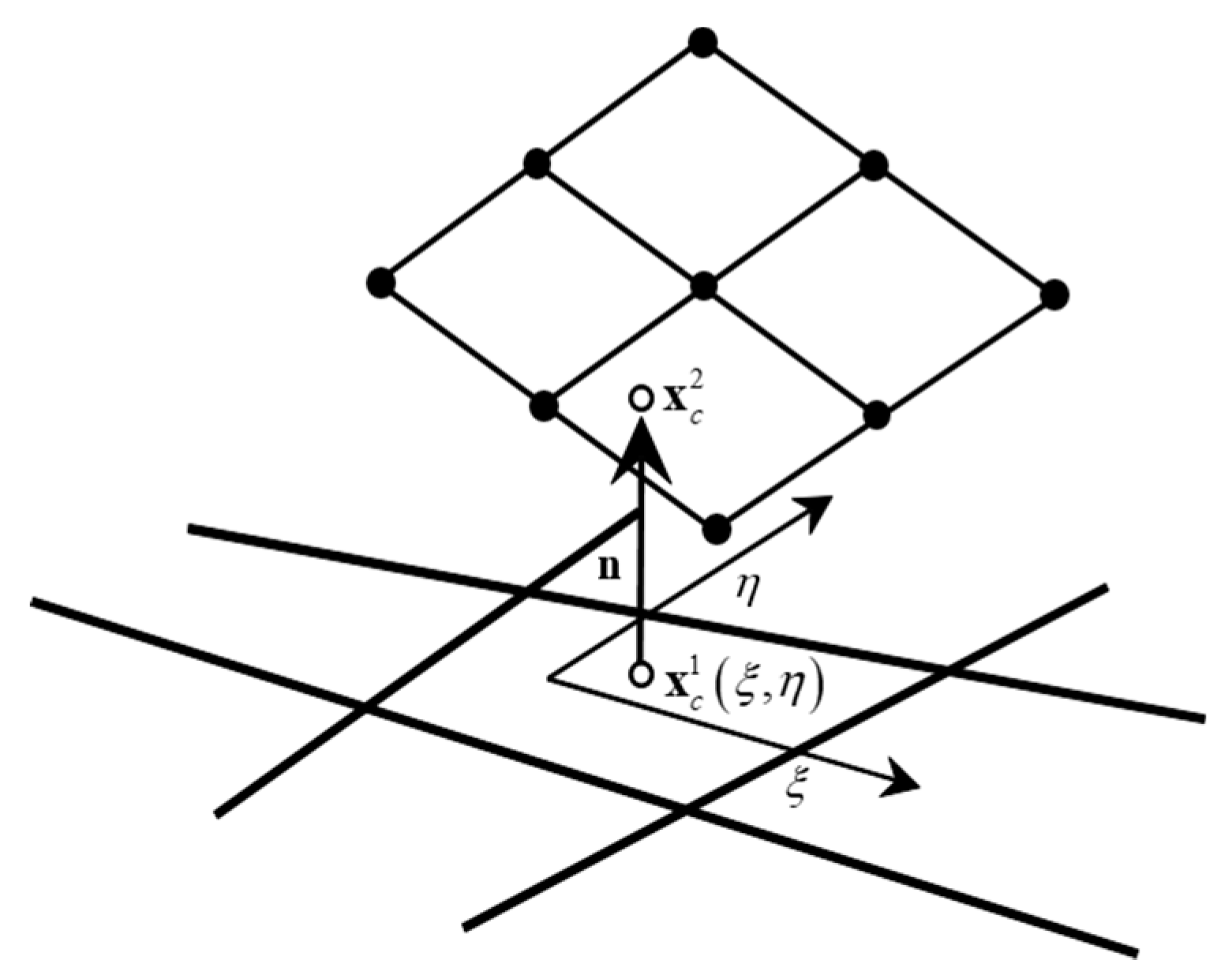
In implementing the contact algorithm at the interface, the mortar method [18] with element-based integration was adopted. Let us define the pad and disc interface as a slave (nonmortar) and master (mortar) segment. At each integration point of the slave segment, orthogonal projection is applied to find the master segment and its natural coordinate. A graphical interpretation is presented in Figure 2, this relationship may be formulated with the following nonlinear equations.

$$\begin{array}{l}{x}_{c,\xi }^1\left({\xi }_c,{\eta }_c\right)\cdot \left(x_c^2-x_c^1\left({\xi }_c,{\eta }_c\right)\right)=0\\ x_{c,\eta }^1\left({\xi }_c,{\eta }_c\right)\cdot \left(x_c^2-x_c^1\left({\xi }_c,{\eta }_c\right)\right)=0\end{array}$$

(1)

where $x_c^2,x_c^1\left({\xi }_c,{\eta }_c\right)$ are the contact point of the slave and master segment. Since Equation (1) is nonlinear, the iterative procedure based on Newton’s method is applied. The associated linearization can be expressed as

$$\left[\begin{array}{cc}{x}_{c,\xi }^1\cdot x_{c,\xi }^1-x_{c,\xi \xi }^1\cdot \left(x_c^2-x_c^1\right)& x_{c,\xi }^1\cdot x_{c,\eta }^1-x_{c,\xi \eta }^1\cdot \left(x_c^2-x_c^1\right)\\ x_{c,\xi }^1\cdot x_{c,\eta }^1-x_{c,\xi \eta }^1\cdot \left(x_c^2-x_c^1\right)& x_{c,\eta }^1\cdot x_{c,\eta }^1-x_{c,\eta \eta }^1\cdot \left(x_c^2-x_c^1\right)\end{array}\right]\left[\begin{array}{c}\mathrm{\Delta }{\xi }_c\\ \mathrm{\Delta }{\eta }_c\end{array}\right]=\left[\begin{array}{c}{x}_{c,\xi }^1\cdot \left(x_c^2-x_c^1\right)\\ x_{c,\eta }^1\cdot \left(x_c^2-x_c^1\right)\end{array}\right]$$

(2)

where the row vectors $x_{c,\xi }^1,x_{c,\eta }^1$ are derivative of $x_c^1$ with respect to $\xi ,\eta$, and $x_{c,\xi \xi }^1,x_{c,\xi \eta }^1$, and $x_{c,\eta \eta }^1$ are second derivative of $x_c^1$. In determining the contact status, this paper assumes that all integration points at the interface are in contact and tangentially sliding. Utilizing the linear force relationship and Coulomb’s friction law, the normal and tangential contact force are modeled as follows:

$$\begin{array}{l}{F}_n=k_L\left(u_p-u_d\right)\\ F_t=\mu F_n\end{array}$$

(3)

where $F_n,F_t$ are normal and tangential contact force, and $k_L,u_p,u_d,$ and $\mu$ are normal contact stiffness, displacement of the pad and disc, and the friction coefficient, respectively. Throughout this paper, normal contact stiffness, i.e., $k_L={10}^{16}$, is used. Based on the contact points and force relation, the normal and tangential stiffness matrices of each contact segment are given by [19]

$$\begin{array}{l}{K}_{\mathrm{N}}=k_L{\displaystyle \sum _{i=1}^{N_{\mathrm{int}}}{w}_i{N}_n^{\mathrm{T}}\left({\xi }_i,{\eta }_i\right)N_n\left({\xi }_i,{\eta }_i\right)}\det \left(J\right)\\ K_{\mathrm{T}}=\mu k_L{\displaystyle \sum _{i=1}^{N_{\mathrm{int}}}{w}_i{N}_t^{\mathrm{T}}\left({\xi }_i,{\eta }_i\right)N_n\left({\xi }_i,{\eta }_i\right)}\det \left(J\right)\end{array}$$

(4)

where $w_i,\det \left(J\right)$ are the integration weight, and determinant of the Jacobian, and $N_n,N_t$ are the matrices related to normal and tangential directions. Since only hexahedral elements are used in this example, all interface segments are quadrilateral, and matrices $N_n,N_t$ are expressed as follows:

$$\begin{array}{ll}{N}_t& =\left[\begin{array}{cc}{x}_{c,\xi }^1\cdot v/\left|v\right|& x_{c,\eta }^1\cdot v/\left|v\right|\end{array}\right]{\left[\begin{array}{cc}{x}_{c,\xi }^1\cdot x_{c,\xi }^1& x_{c,\xi }^1\cdot x_{c,\eta }^1\\ x_{c,\xi }^1\cdot x_{c,\eta }^1& x_{c,\eta }^1\cdot x_{c,\eta }^1\end{array}\right]}^{-1}\left[\begin{array}{c}{N}_{t\xi }\\ N_{t\eta }\end{array}\right]\\ N_n& =\left[\begin{array}{ccccc}{N}_1\left({\xi }_i,{\eta }_i\right)n& N_2\left({\xi }_i,{\eta }_i\right)n& N_3\left({\xi }_i,{\eta }_i\right)n& N_4\left({\xi }_i,{\eta }_i\right)n& 0\end{array}\right]\\ & -\left[\begin{array}{ccccc}0& N_1\left({\xi }_c,{\eta }_c\right)n& N_2\left({\xi }_c,{\eta }_c\right)n& N_3\left({\xi }_c,{\eta }_c\right)n& N_4\left({\xi }_c,{\eta }_c\right)n\end{array}\right]\\ N_{t\alpha }& =\left[\begin{array}{ccccc}{N}_1\left({\xi }_i,{\eta }_i\right)x_{c,\alpha }^1& N_2\left({\xi }_i,{\eta }_i\right)x_{c,\alpha }^1& N_3\left({\xi }_i,{\eta }_i\right)x_{c,\alpha }^1& N_4\left({\xi }_i,{\eta }_i\right)x_{c,\alpha }^1& 0\end{array}\right]\\ & -\left[\begin{array}{ccccc}0& N_1\left({\xi }_c,{\eta }_c\right)x_{c,\alpha }^1& N_2\left({\xi }_c,{\eta }_c\right)x_{c,\alpha }^1& N_3\left({\xi }_c,{\eta }_c\right)x_{c,\alpha }^1& N_4\left({\xi }_c,{\eta }_c\right)x_{c,\alpha }^1\end{array}\right],\alpha =\xi ,\eta \end{array}$$

(5)

where $n,0,v/\left|v\right|$ and $N_i$ are the normal row vector, zero row vector with size 12, the directional velocity at the contact point, and i-th shape function.

Based on the contact stiffness and system matrices of the disc and pad, the deterministic eigenvalue problem can be expressed as

$$\left[K+{\lambda }_{i}C+{\lambda }_i^{2}M\right]{\Phi }_i=0$$

(6)

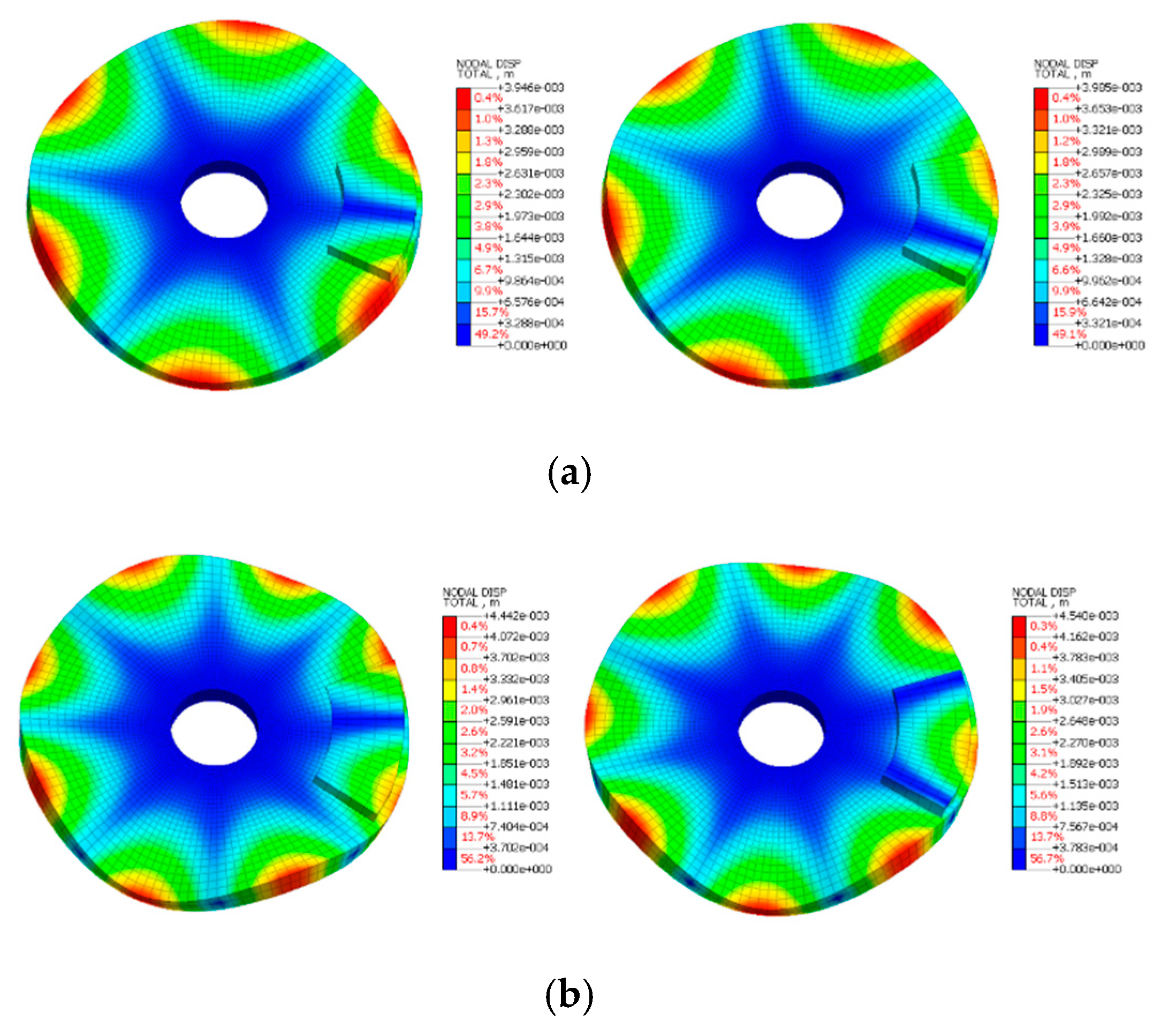
where $M,C,$ and $K$ are mass, damping, and stiffness matrix, respectively. To investigate the eigenvalue characteristic, Equation (6) is solved for the friction coefficient $\mu =0.8$ and in the absence of damping. The obtained first two unstable eigensolution pair results are presented in Figure 3.

Since the tangential contact stiffness matrix is nonsymmetric, the eigensolutions can become complex values, even without damping. The real part of the eigenvalue corresponds to the dynamic response caused by the instability. If the given system has all the negative real parts of the eigenvalues, the system is considered stable. However, if at least one of them is positive, the system is regarded as unstable.

2.2. Stochastic Complex Eigenvalue Analysis under Uncertainties

If some structure parts have parametric uncertainties, they can be modeled by introducing additional terms to the deterministic system. Let $\mathsf{\Theta },\mathcal{F},\mathcal{P}$ denotes the probability spaces, where $\mathsf{\Theta },\mathcal{F}$ and $\mathcal{P}$ are the sample space, σ-algebra, and probability measure of M random variables $\zeta =\left({\zeta }_1,{\zeta }_2,\dots {\zeta }_M\right),$ respectively. If the uncertainty is modeled as a spatially-distributed field, the random field can be represented by spectral decomposition using a truncated Karhunen-Loève (KL) expansion [20]. Based on the modeled random variable, each system matrix is represented as a combination of the deterministic and random matrix as follows:

$$M\left(\zeta \right)=M_0+{\displaystyle {\sum }_{i=1}^{n_1}{M}_i\left(\zeta \right)},C\left(\zeta \right)=C_0+{\displaystyle {\sum }_{i=1}^{n_2}{C}_i\left(\zeta \right)},K\left(\zeta \right)=K_0+{\displaystyle {\sum }_{i=1}^{n_3}{K}_i\left(\zeta \right)}$$

(7)

where $M\left(\zeta \right),C\left(\zeta \right),$ and $K\left(\zeta \right)$ are random mass, damping, and stiffness matrix. The subscripts zero and i represent the deterministic and i-th random matrix, and n₁, n₂, and n₃ indicate the number of random variables in each system matrix, respectively. Utilizing the obtained random system matrices, the stochastic eigenvalue problem can be expressed as

$$\left[K\left(\zeta \right)+{\lambda }_i\left(\zeta \right)C\left(\zeta \right)+{\lambda }_i^2\left(\zeta \right)M\left(\zeta \right)\right]{\Phi }_i\left(\zeta \right)=0$$

(8)

where ${\lambda }_i\left(\zeta \right),{\Phi }_i\left(\zeta \right)$ are the i-th random eigenvalue and eigenvector.

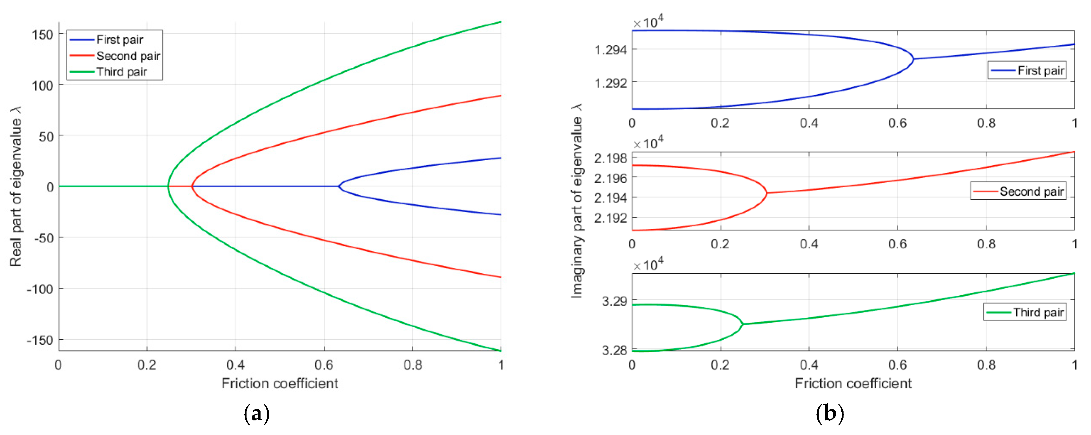
Prior to describing the proposed method for the stochastic eigenvalue problem, the response due to the friction coefficient is computed. In the absence of damping, the first three unstable eigenvalue pairs within the friction coefficient interval $\left[0,1\right]$ are shown in Figure 4.

It can be seen from the results that after the critical friction coefficient, the two real eigenvalues are separated (bifurcation), while the imaginary parts coalesce (mode-coupling). Near the critical point, the first derivative of eigenvalues may not be continuous and, after this point, the response patterns are changed. Also, this coalescence pattern can be changed by the effect of damping [3]. Let $c_k=2{\chi }_k{\omega }_k$ be the structure damping associated with an unstable eigenvalue pair, where ${\omega }_k$ is the natural frequency without friction and ${\chi }_k$ is the modal damping ratio. If damping is equal on the two coupling modes (i.e., $c_1=c_2$), it will lower the real part curves, whereas the coalescence point is still singular. However, if damping is nonequally distributed (i.e., $c_1\ne c_2$), the coalescence is not perfect, and the imaginary parts will not be the same at a critical point. In this paper, only singular-coalescence point cases (e.g., undamped and equally damped) are considered.

3. Proposed Algorithm

3.1. Nonstationary Kriging

As described in the previous section, complex eigenvalues show heterogeneous behavior near the bifurcation point. Since stationary kriging is based on the assumption that the response smoothness is fairly uniform, application to brake systems is still limited. To address this issue, the nonstationary kriging algorithm is presented. For simplicity, let $\mathcal{M}\left(\zeta \right)$ be the model problem in Equation (8) and y the interested eigenvalue result. Using this notation, the random eigenvalue problem can be simply expressed as $y=\mathcal{M}\left(\zeta \right)$. Given N samples $\left\{{\zeta }^1,\dots {\zeta }^N\right\}$ in the M dimensional input space and their associated output $\left\{y^1,\dots y^N\right\}$, the kriging assumes that the response of a computational model is a realization of the Gaussian random process as

$$y=\mathcal{M}\left(\zeta \right)\simeq f^{\mathrm{T}}\left(\zeta \right)\mathsf{\beta }+Z\left(\zeta \right)$$

(9)

where the first part $f\left(\zeta \right),\mathsf{\beta }$ represents the trend function, and their product is the mean of the response. In constructing a global trend, ordinary kriging uses a constant value, while universal kriging uses polynomial functions. The second part $Z\left(\zeta \right)$ is a Gaussian process with zero mean satisfying the following statistical property:

$$\mathbb{E}\left[Z\left({\zeta }^i\right)Z\left({\zeta }^j\right)\right]={\sigma }^{2}R\left({\zeta }^i,{\zeta }^j\right)$$

(10)

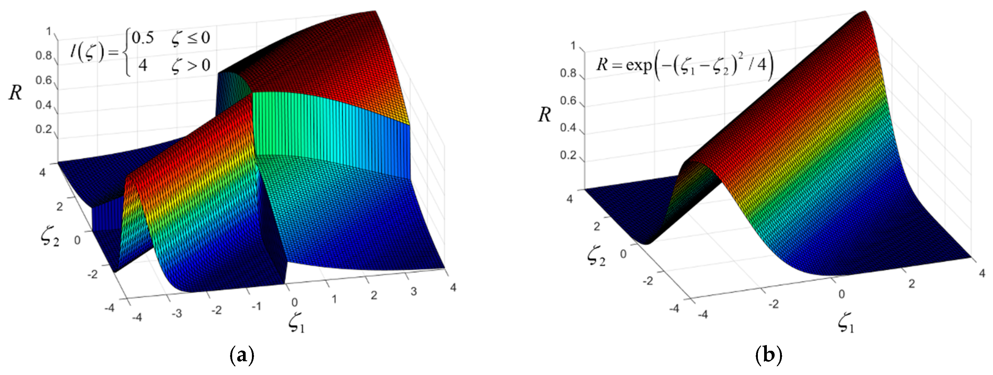
where ${\sigma }^2,R\left({\zeta }^i,{\zeta }^j\right)$, and ${\zeta }^i$ are the process variance of $Z\left(\zeta \right)$, the correlation function, and i-th input sample. In selecting the correlation function in the conventional stationary kriging, the Gaussian type $R\left({\zeta }^i,{\zeta }^j\right)={\displaystyle {\prod }_{k=1}^M\exp \left(-{\mathsf{\theta }}_k{\left({\zeta }^i-{\zeta }^j\right)}^2\right)}$ is widely used. However, rather than applying the stationary kernel, the following nonstationary Gibbs kernel [21] is adopted.

$$R\left({\zeta }^i,{\zeta }^j\right)={\displaystyle \prod _{k=1}^M{\left(\frac{2l_k\left({\zeta }^i\right)l_k\left({\zeta }^j\right)}{l_k^2\left({\zeta }^i\right)+l_k^2\left({\zeta }^j\right)}\right)}^{1/2}\exp \left(-\frac{{\left({\zeta }^i-{\zeta }^j\right)}^2}{l_k^2\left({\zeta }^i\right)+l_k^2\left({\zeta }^j\right)}\right)}$$

(11)

where $l_k(\cdot )$ is the length-scale in k-th input dimension. The length-scale controls the response smoothness within the input domain, and can be any arbitrary positive function of random variables $\zeta$. In this paper, to reflect the heterogeneous properties in each stable and unstable regions, the length-scale for the input sample is modeled by using step-wise hyperparameters as follows:

$$l_k\left({\zeta }^i\right)=\{\begin{array}{cc}{\mathsf{\theta }}_k^1& g\left({\zeta }^i\right)=0\\ {\mathsf{\theta }}_k^2& g\left({\zeta }^i\right)>0\end{array}$$

(12)

where $g\left({\zeta }^i\right),\mathsf{\theta }$ are the criteria function and hyperparameter to be determined. Based on the fact that the real eigenvalue pair ${\lambda }_1,{\lambda }_2$ is bifurcate after the mode-coupling, the following stability criteria function is proposed.

$$g\left({\zeta }^i\right)=\left|\mathrm{Re}\left({\lambda }_1\left({\zeta }^i\right)\right)-\mathrm{Re}\left({\lambda }_2\left({\zeta }^i\right)\right)\right|$$

(13)

The proposed function can be interpreted as a gap between two eigenvalues. If $g\left({\zeta }^i\right)=0$, the given eigenvalue pair is stable, and if $g\left({\zeta }^i\right)>0$, instability occurs. A simple comparison of nonstationary and stationary correlation functions is presented in Figure 5. For a stationary correlation function, the Gaussian type is considered. By comparing these two results, the proposed kernel and length scale function makes it possible to model the heterogeneity of the response. If the length-scale is relatively high, the response is smooth, whereas if the length-scale is low, the response changes rapidly. However, for a stationary correlation function, the entire input space is correlated.

After the input samples are divided by utilizing the criteria function in Equation (13), the correlation matrix based on the given N samples is constructed as

$$R\left({\zeta }^i,{\zeta }^j\right)=\left[\begin{array}{ccc}R\left({\zeta }^1,{\zeta }^1\right)& \dots & R\left({\zeta }^1,{\zeta }^N\right)\\ ⋮& \ddots & ⋮\\ R\left({\zeta }^N,{\zeta }^1\right)& \dots & R\left({\zeta }^N,{\zeta }^N\right)\end{array}\right]$$

(14)

The kriging model parameters are computed using the best linear unbiased estimator (BLUE) [22] given by

$$\begin{array}{l}\mathsf{\beta }={\left(F^{\mathrm{T}}{R}^{-1}F\right)}^{-1}{F}^{\mathrm{T}}{R}^{-1}y\\ {\sigma }^2=\left[{\left(y-F\mathsf{\beta }\right)}^{\mathrm{T}}{R}^{-1}\left(y-F\mathsf{\beta }\right)\right]/N\end{array}$$

(15)

The hyperparameters are obtained by solving an optimization problem that minimizes the concentrated log-likelihood function as follows:

$$\psi \left(\mathsf{\theta }\right)=\frac{1}{2}\ln \left|R\left(\mathsf{\theta }\right)\right|+\frac{N}{2}\ln \left({\sigma }^2\left(\mathsf{\theta }\right)\right)$$

(16)

In solving the problem in Equation (16), the pattern search, which is one of the global optimization algorithms, is adopted. After obtaining hyperparameters, the predicted response and its variance at the unsampled input point $\zeta$ are computed as

$$\begin{array}{l}y\left(\zeta \right)\simeq f^{\mathrm{T}}\left(\zeta \right)\mathsf{\beta }+r^{\mathrm{T}}\left(\zeta \right)R^{-1}\left(y-F\mathsf{\beta }\right)\\ {\widehat{\sigma }}^2\left(\zeta \right)={\sigma }^2\left(1-\left[\begin{array}{cc}{f}^{\mathrm{T}}\left(\zeta \right)& r^{\mathrm{T}}\left(\zeta \right)\end{array}\right]{\left[\begin{array}{cc}0& F^{\mathrm{T}}\\ F& R\end{array}\right]}^{-1}\left[\begin{array}{c}f\left(\zeta \right)\\ r\left(\zeta \right)\end{array}\right]\right)\end{array}$$

(17)

where $r\left(\zeta \right)$ is the correlation vector between input $\zeta$ and given N samples, and its i-th component is

$$r_i\left(\zeta \right)=R\left(\zeta ,{\zeta }^i\right)={\displaystyle \prod _{k=1}^M{\left(\frac{2{\tilde{l}}_k\left(\zeta \right)l_k\left({\zeta }^i\right)}{{\tilde{l}}_k^2\left(\zeta \right)+l_k^2\left({\zeta }^i\right)}\right)}^{1/2}\exp \left(-\frac{{\left(\zeta -{\zeta }^i\right)}^2}{{\tilde{l}}_k^2\left(\zeta \right)+l_k^2\left({\zeta }^i\right)}\right)}$$

(18)

where ${\tilde{l}}_k\left(\zeta \right)$ is the k-th length-scale for the unsampled input $\zeta$.

One difference between stationary kriging and the proposed method is that, in the case of stationary kriging, one can estimate the response for any input using Equation (17). However, for nonstationary kriging, the correlation function in Equation (18) cannot be constructed, since the length scale function for unsampled input is unknown. As a result, the response prediction in Equation (17) is not directly applicable. To tackle this issue, support vector machine (SVM) -based classification for unsampled input is applied and will be discussed in the next subsection.

3.2. SVM Based Classification for Predicting the Response

The SVM [23] has been widely used for solving both linear and nonlinear classification problems. It uses a binary decision that maps given samples (training data) to a discrete-valued output class $z\in \left\{-1,1\right\}$. Since the eigenvalues of the brake system have two states, i.e., either stable or unstable, the SVM can be directly applied. In this paper, the classes $z=-1$ and $z=1$ are defined as to the region where stable and unstable response occur. Given N samples and their obtained output class using the stability criteria function, a hyperplane equation which separates these two classes can be constructed as follows:

$$h\left(\zeta \right)=b+{\displaystyle \sum _{i=1}^N{\alpha }_i{z}^{i}K\left({\zeta }^i,\zeta \right)}$$

(19)

where $b,K\left({\zeta }^i,\zeta \right),z^i$ and ${\alpha }_i$ are the intercept with the origin, kernel function of the SVM, output class of i-th sample, and Lagrange multipliers, respectively. In applying the kernel function for the SVM, a Gaussian-type function is adopted in this paper. The Lagrange multipliers are unknown and can be obtained by maximizing the margin between support hyperplanes. After Lagrange multipliers are computed, the hyperplane is given by $h\left(\zeta \right)=0$, and output classes of −1 and 1 are predicted by $h\left(\zeta \right)<0$ and $h\left(\zeta \right)>0$, respectively. Utilizing the SVM classification, k-th length scale for the given unsampled input point is estimated as

$${\tilde{l}}_k\left(\zeta \right)=\{\begin{array}{cc}{\theta }_k^1& h\left(\zeta \right)<0\\ {\theta }_k^2& h\left(\zeta \right)>0\end{array}$$

(20)

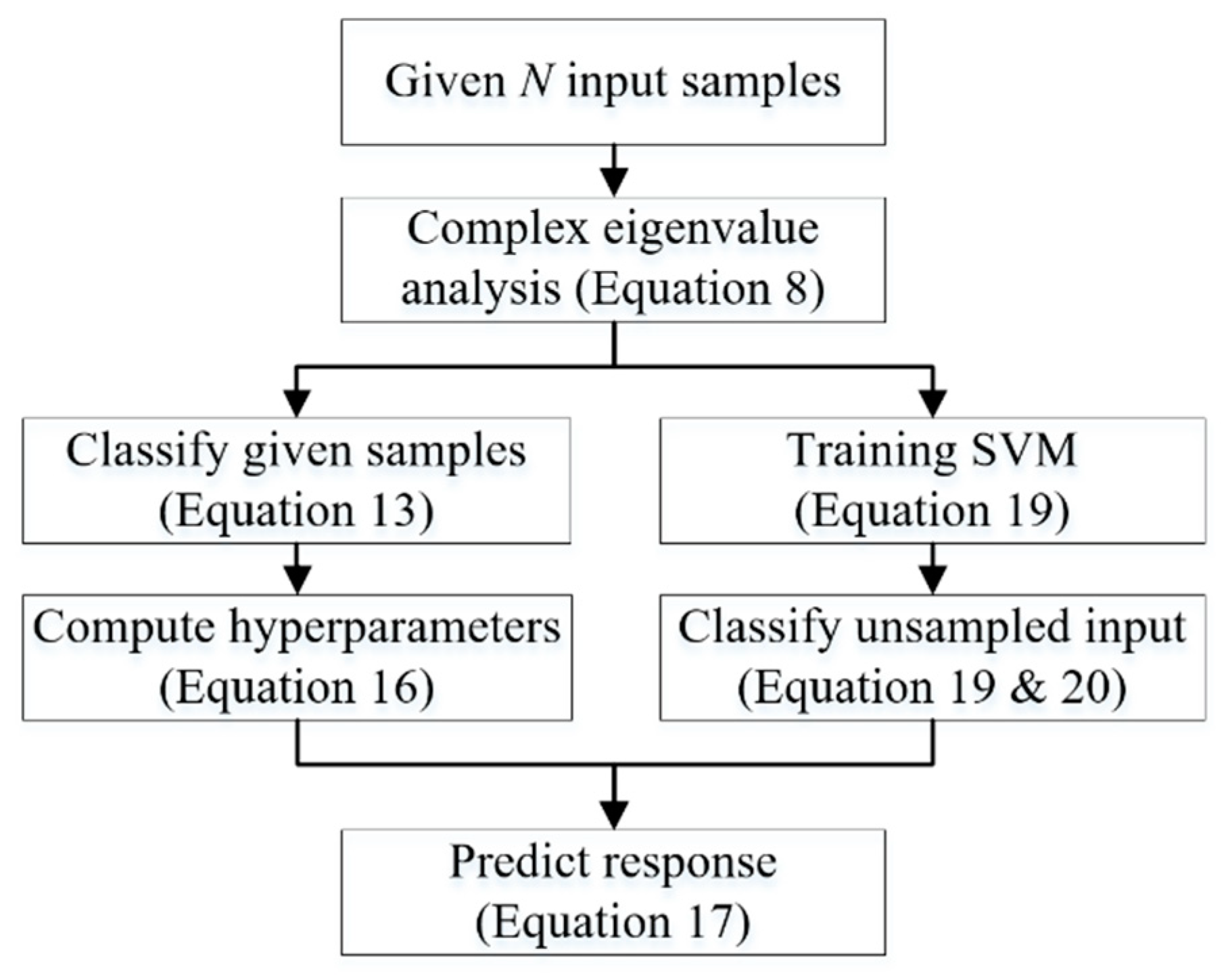
Since the length-scale for unsampled input is now defined, the response prediction for nonstationary kriging in Equation (17) can be computed. A flowchart of the proposed combined nonstationary kriging and SVM method is presented in Figure 6.

In comparison with stationary kriging, the proposed algorithm increases the number of hyperparameters in optimization problems and requires SVM training. However, if the complex eigenvalue problem requires a large amount of computation, these additional operations can be ignored compared to solving the eigenvalue problem. Issues regarding the accuracy and computational efficiency of the proposed method will be discussed in the next section.

4. Numerical Results

Prior to validating the proposed method through numerical studies, some implementation issues and the development environments are briefly discussed. All the algorithms mentioned above are developed with in-house code, written in the MATLAB 2017Ra. In performing some numerical operations, the following MATLAB commands are used: eigs for solving eigenvalue problems, patternsearch for optimization in kriging, fitcsvm for training support vector machine, and ksdensity for estimating the probability density function (PDF). In stationary kriging, the Gaussian type correlation function is applied. Finally, the numerical simulations are carried out on a personal desktop operating Windows 10 with Intel Core [email protected] GHz and 16 GB RAM.

4.1. Case 1: Study with a Random Friction Coefficient

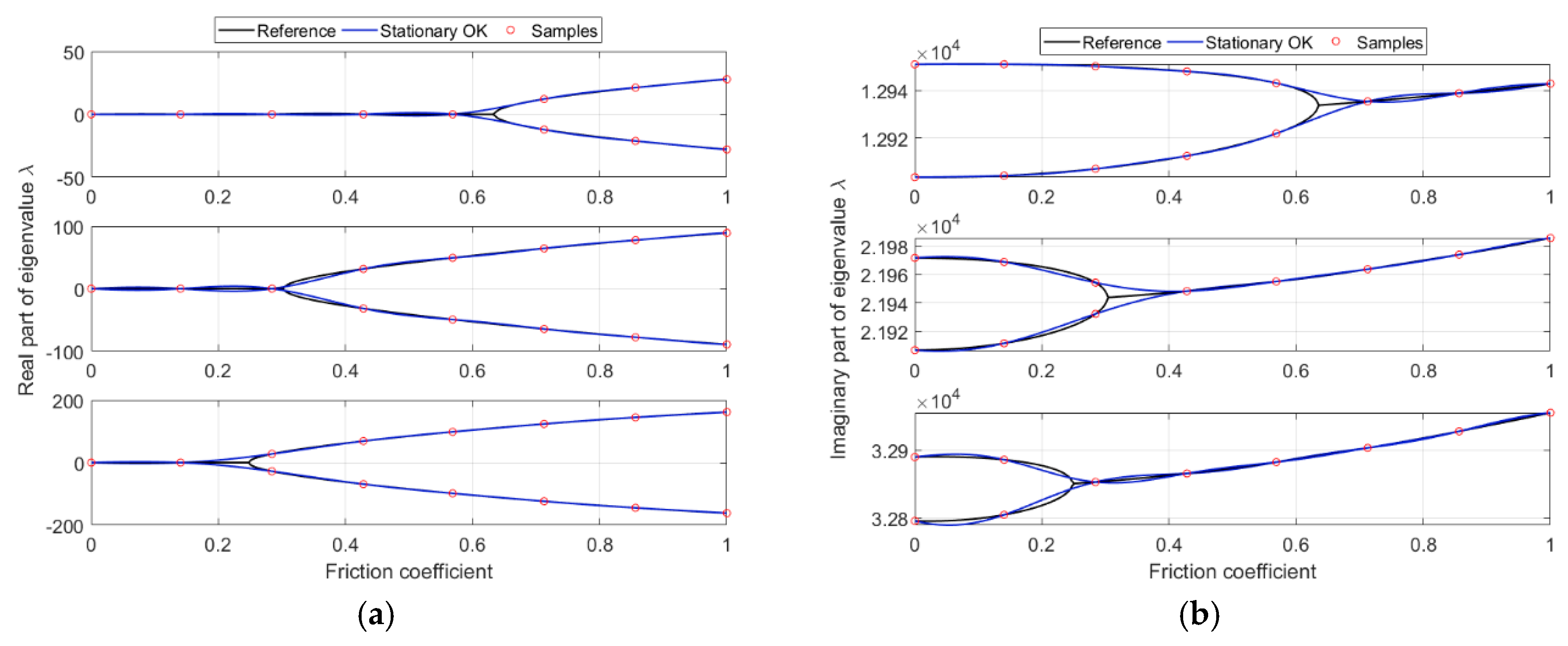
In the first case study, only the friction coefficient is considered as a random variable. The eigenvalue results and their solution characteristics have already been discussed in Section 2.2. The purpose of this simple case study is to test the stationary kriging in nonstationary environment and validate our proposed kernel with length-scale function. Using eight equally-spaced samples within the interval $\left[0,1\right]$, the stationary ordinary kriging (i.e., constant trend function) is applied. The first three unstable eigenvalue pairs are presented in Figure 7. In obtaining the reference results, 300 equally-spaced samples are considered.

As seen in the results, the samples are far away from the bifurcation point. Therefore, the transition region near this point is not reflected, and except for that region, the obtained results show quite good agreement with reference. In order to investigate the effect of the trend functions, the polynomial trend functions from 0th to 3rd order are applied; the error results are given in

Table 2. Error results for the three unstable eigenvalue pairs using the stationary kriging with eight samples. The trend functions with polynomial order from 0th to 3rd are applied.

	$\mathbf{Re}\left({\mathit{\lambda }}_1\right)$	$\mathbf{Re}\left({\mathit{\lambda }}_2\right)$	$\mathbf{Re}\left({\mathit{\lambda }}_3\right)$	$\mathbf{Im}\left({\mathit{\lambda }}_1\right)$	$\mathbf{Im}\left({\mathit{\lambda }}_2\right)$	$\mathbf{Im}\left({\mathit{\lambda }}_3\right)$	${\displaystyle \sum \mathbf{Re}\left({\mathit{\lambda }}_{\mathit{i}}\right)}$	${\displaystyle \sum \mathbf{Im}\left({\mathit{\lambda }}_{\mathit{i}}\right)}$
0th	6.72 × 10−2	3.95 × 10−2	3.54 × 10−2	7.26 × 10−5	8.29 × 10−5	8.72 × 10−5	1.42 × 10−1	2.43 × 10−4
1st	7.00 × 10−2	3.98 × 10−2	3.47 × 10−2	7.32 × 10−5	8.00 × 10−5	1.18 × 10−4	1.45 × 10−1	2.72 × 10−4
2nd	1.54 × 10−1	3.84 × 10−2	3.51 × 10−2	7.35 × 10−5	1.61 × 10−4	1.47 × 10−4	2.27 × 10−1	3.81 × 10−4
3rd	1.56 × 10−1	4.78 × 10−2	3.55 × 10−2	1.19 × 10−4	1.61 × 10−4	1.30 × 10−4	2.39 × 10−1	4.11 × 10−4

. In evaluating the error, the following 2-norm error is considered.

$${\epsilon }_{2-\mathrm{norm}}=\sqrt{{\displaystyle \sum _{j=1}^2{\displaystyle \sum _{i=1}^N{\left({\lambda }_{\mathrm{kriging}}^{i,j}-{\lambda }_{\mathrm{ref}}^{i,j}\right)}^2}}}/\sqrt{{\displaystyle \sum _{i=1}^2{\displaystyle \sum _{j=1}^N{\left({\lambda }_{\mathrm{ref}}^{i,j}\right)}^2}}}$$

(21)

where superscripts i and j denote the j-th part of the eigenvalue pair in the i-th sample. The results indicate that the 0th order trend function shows the best performance under the given samples.

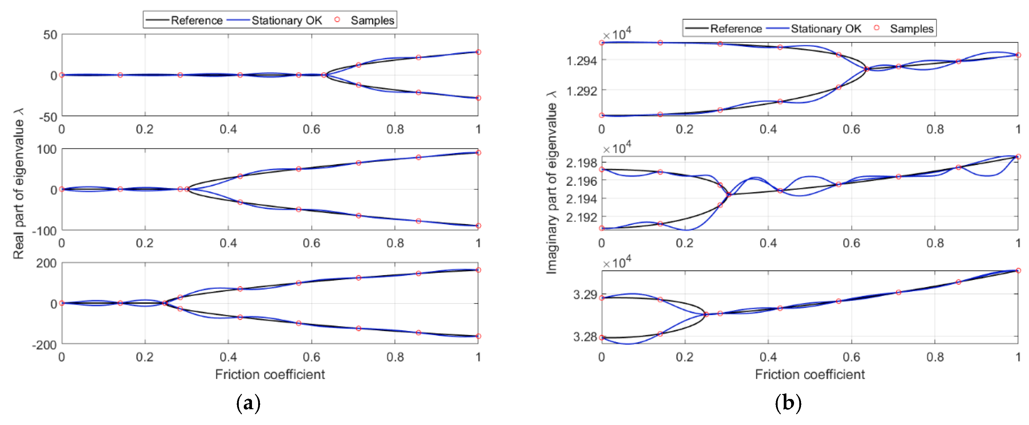
Next, near each bifurcation point of unstable eigenvalues, an additional sample is introduced. The first three unstable eigenvalue pairs using ordinary kriging are shown in Figure 8. The obtained results show that although the total number of samples is increased, their accuracy is severely degraded. Reflecting the nonsmooth characteristic at the bifurcation point results in inaccurate oscillations over the input range. This implies that the response prediction can be highly sensitive to the sample near the bifurcation point. In order to compare the error, metamodels for different trend functions are computed; the error results are presented in

Table 3. Error results for the three unstable eigenvalue pairs using the stationary kriging with nine samples. The trend functions with polynomial order from 0th to 3rd are applied.

	$\mathbf{Re}\left({\mathit{\lambda }}_1\right)$	$\mathbf{Re}\left({\mathit{\lambda }}_2\right)$	$\mathbf{Re}\left({\mathit{\lambda }}_3\right)$	$\mathbf{Im}\left({\mathit{\lambda }}_1\right)$	$\mathbf{Im}\left({\mathit{\lambda }}_2\right)$	$\mathbf{Im}\left({\mathit{\lambda }}_3\right)$	${\displaystyle \sum \mathbf{Re}\left({\mathit{\lambda }}_{\mathit{i}}\right)}$	${\displaystyle \sum \mathbf{Im}\left({\mathit{\lambda }}_{\mathit{i}}\right)}$
0th	1.16 × 10−1	8.36 × 10−2	8.46 × 10−2	1.30 × 10−4	2.94 × 10−4	1.85 × 10−4	2.84 × 10−1	6.09 × 10−4
1st	9.44 × 10−2	5.56 × 10−2	5.24 × 10−2	1.90 × 10−4	2.75 × 10−4	1.40 × 10−4	2.02 × 10−1	6.05 × 10−4
2nd	7.92 × 10−2	5.33 × 10−2	5.37 × 10−2	6.87 × 10−5	1.84 × 10−4	1.13 × 10−4	1.86 × 10−1	3.66 × 10−4
3rd	8.57 × 10−2	4.50 × 10−2	4.58 × 10−2	1.30 × 10−4	1.82 × 10−4	1.16 × 10−4	1.77 × 10−1	4.28 × 10−4

. Comparing Table 2 and Table 3, the results under given samples indicate that applying a high-order trend function may increase the metamodel performance. However, the accuracy is not always guaranteed, and depending on the response characteristics, their optimal polynomial orders differ

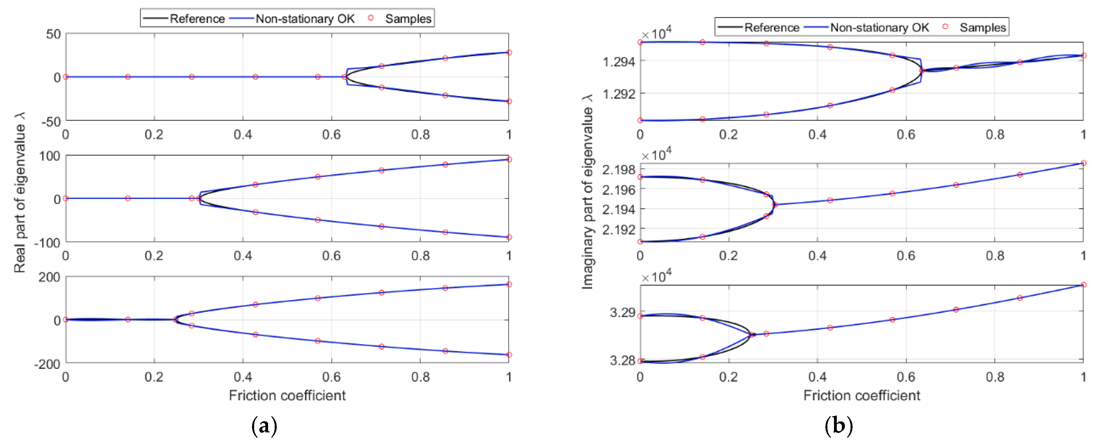
Finally, our proposed method is applied. In this case, only the nonstationary kernel with length-scale function is examined. Rather than using the SVM to classify the unsampled input, an additional sample acts as a hyperplane. The first three unstable eigenvalue pairs using ordinary kriging are given in Figure 9, the error results for different trend functions are listed in

Table 4. Error results for the three unstable eigenvalue pairs using the nonstationary kriging with nine samples. The trend functions with polynomial order from 0th to 3rd are applied.

	$\mathbf{Re}\left({\mathit{\lambda }}_1\right)$	$\mathbf{Re}\left({\mathit{\lambda }}_2\right)$	$\mathbf{Re}\left({\mathit{\lambda }}_3\right)$	$\mathbf{Im}\left({\mathit{\lambda }}_1\right)$	$\mathbf{Im}\left({\mathit{\lambda }}_2\right)$	$\mathbf{Im}\left({\mathit{\lambda }}_3\right)$	${\displaystyle \sum \mathbf{Re}\left({\mathit{\lambda }}_{\mathit{i}}\right)}$	${\displaystyle \sum \mathbf{Im}\left({\mathit{\lambda }}_{\mathit{i}}\right)}$
0th	3.35 × 10−2	8.47 × 10−3	1.21 × 10−2	5.93 × 10−5	3.24 × 10−5	1.19 × 10−4	5.42 × 10−2	2.10 × 10−4
1st	3.35 × 10−2	3.06 × 10−2	2.57 × 10−2	9.54 × 10−5	8.85 × 10−5	1.17 × 10−4	8.98 × 10−2	3.01 × 10−4
2nd	4.14 × 10−2	2.00 × 10−2	2.60 × 10−2	5.74 × 10−5	1.52 × 10−4	1.36 × 10−4	8.75 × 10−2	3.45 × 10−4
3rd	4.10 × 10−2	1.57 × 10−2	2.34 × 10−2	1.07 × 10−4	3.81 × 10−5	2.16 × 10−4	8.02 × 10−2	3.61 × 10−4

.

Comparing the results in Figure 8 and Figure 9, the nonstationary kriging results show that the oscillation behaviors are alleviated. This is attributed to a step-wise length scale that reflects the heterogeneity. One observed phenomenon in this example is that the number of samples for the stable region in the third eigenvalue pair is two. Since the given samples are divided based on stability criteria, the number of samples for each region may be insufficient. Therefore, additional sampling may be introduced to increase accuracy.

4.2. Case 2: Study with a Random Friction Coefficient and Young’s Modulus of the Disc

In the second case study, the friction coefficient and Young’s modulus of the disc are considered to be random. Utilizing the random variables, they are modeled as

$$\begin{array}{ll}\mu & =0.5+0.5{\zeta }_1\\ E_{\mathrm{disc}}& =125\times {10}^9\left(1+0.2{\zeta }_2\right)\end{array}$$

(22)

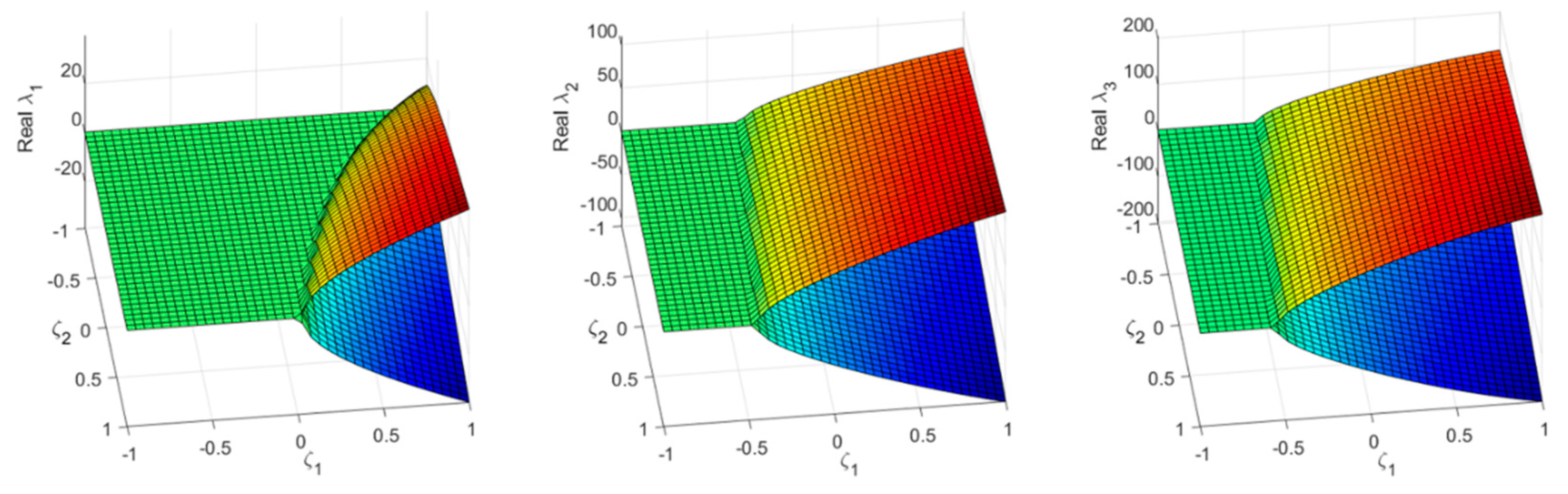
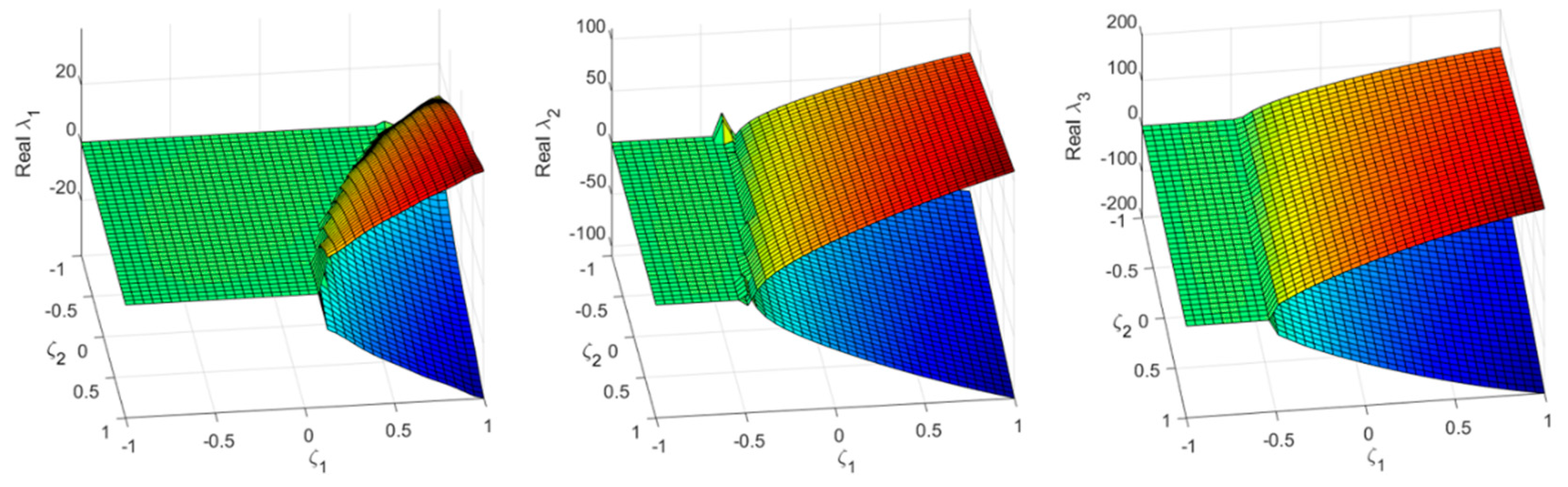
where ${\zeta }_1,{\zeta }_2$ are uniform random variables within the interval $\left[-1,1\right]$. The purpose of the second example is to validate the combined nonstationary kriging and support vector machine method. The reference results for the real part of the first three unstable eigenvalues are presented in Figure 10. In obtaining the reference, a 2D linear sample grid (40 $\times$ 40) is considered. The obtained results show that the sensitivity of the bifurcation friction coefficient to the disk’s random variable is large at the first eigenvalue, making the response surface more complex.

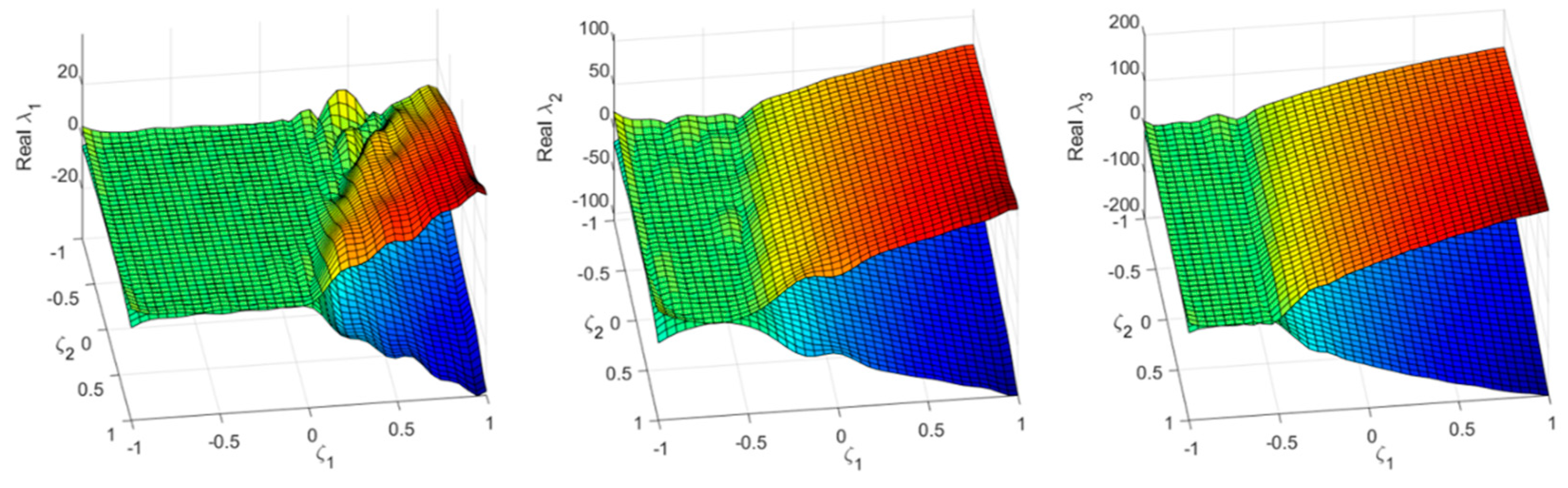
Next, stationary ordinary kriging is applied to create the metamodels. The response surfaces using 150 Sobol sequential samples provided by UQLab [24] are given in Figure 11. It can be seen from the results that the third eigenvalue pair is most accurate, while other pairs show oscillation behavior over the stable region. This is attributed to the fact that for the third eigenvalue pairs, the sensitivity of the bifurcation friction coefficient due to the disk’s parameter is relatively low. Therefore, the response surface has nonstationary characteristics which mainly depend on the friction coefficient. However, for the first and second eigenvalue, nonstationarity exists for both dimensions. Reflecting this behavior under stationarity assumptions results in oscillatory responses.

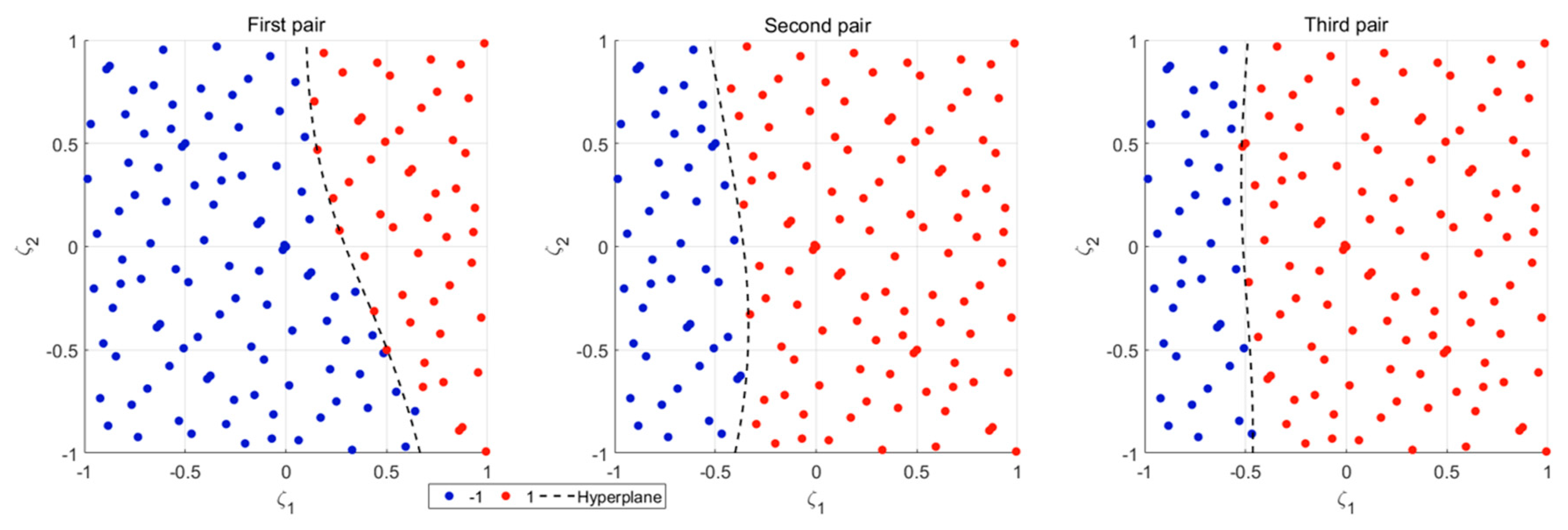
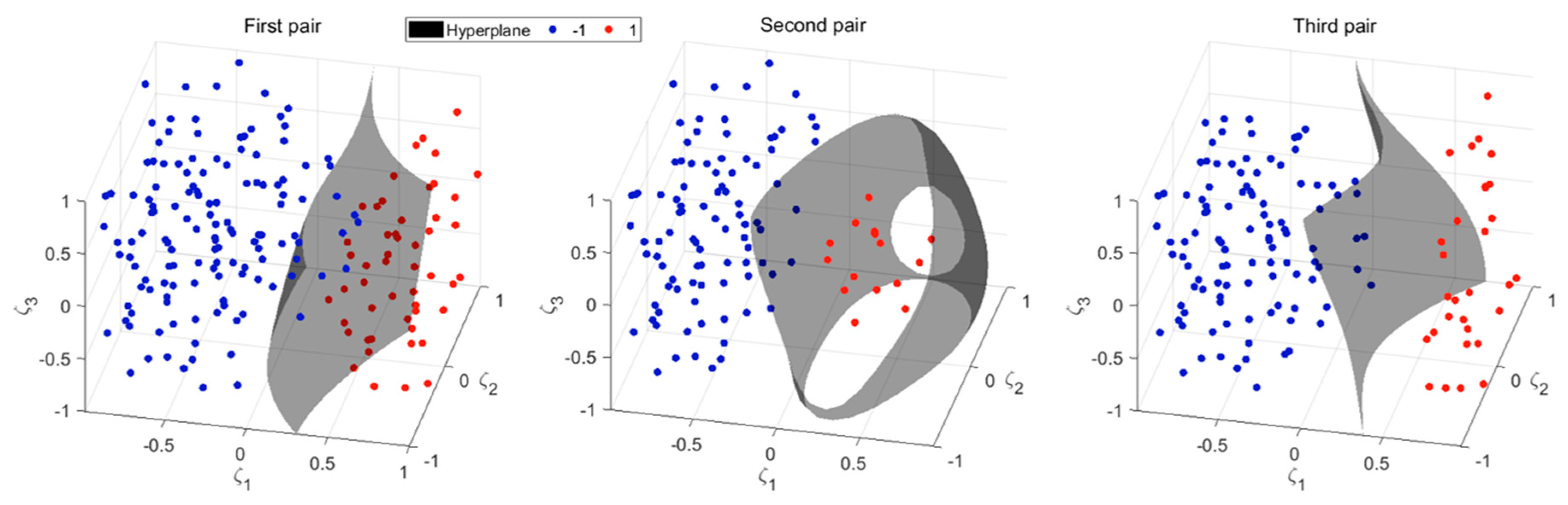
Based on the given 150 samples, our proposed method is applied. The hyperplane results of the SVM for three unstable eigenvalue pairs are shown in Figure 12. Since the Gaussian kernel is applied, the obtained hyperplanes are nonlinear, and can classify the given output classes properly.

After classifying the validated samples utilizing the hyperplane, the predicted response results are presented in Figure 13. The obtained results are quite similar to the reference results in Figure 10, and no spurious oscillations occur. One observed property of the proposed method is that there is a slight peak in the second eigenvalue pair result. This is because the proposed correlation function at the bifurcation boundary is discontinuous. However, this phenomenon can be alleviated by employing additional samples near the boundary.

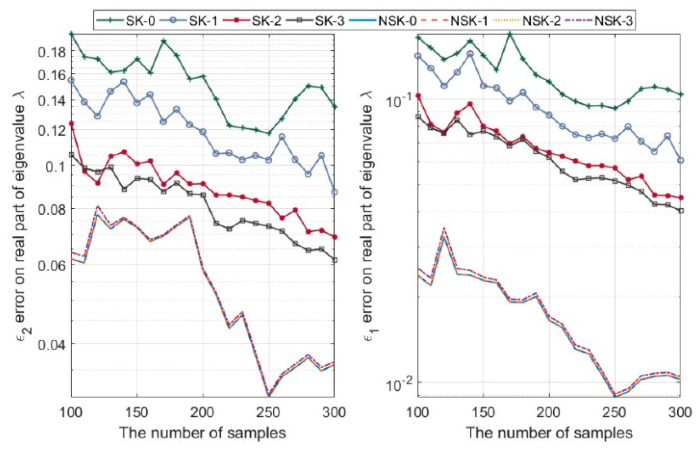
To investigate the error of stationary kriging and the proposed method, the Sobol sequential samplings, from 150 to 300 in increments of 10, are applied. The polynomial trend functions from the 0th to 3rd order are used. In evaluating the error, in addition to the 2-norm based error in Equation (21), the following 1-norm based error is also considered.

$${\epsilon }_{1-\mathrm{norm}}=\sqrt{{\displaystyle \sum _{j=1}^2{\displaystyle \sum _{i=1}^N\left|{\lambda }_{\mathrm{kriging}}^{i,j}-{\lambda }_{\mathrm{ref}}^{i,j}\right|}}}/\sqrt{{\displaystyle \sum _{i=1}^2{\displaystyle \sum _{j=1}^N\left|{\lambda }_{\mathrm{ref}}^{i,j}\right|}}}$$

(23)

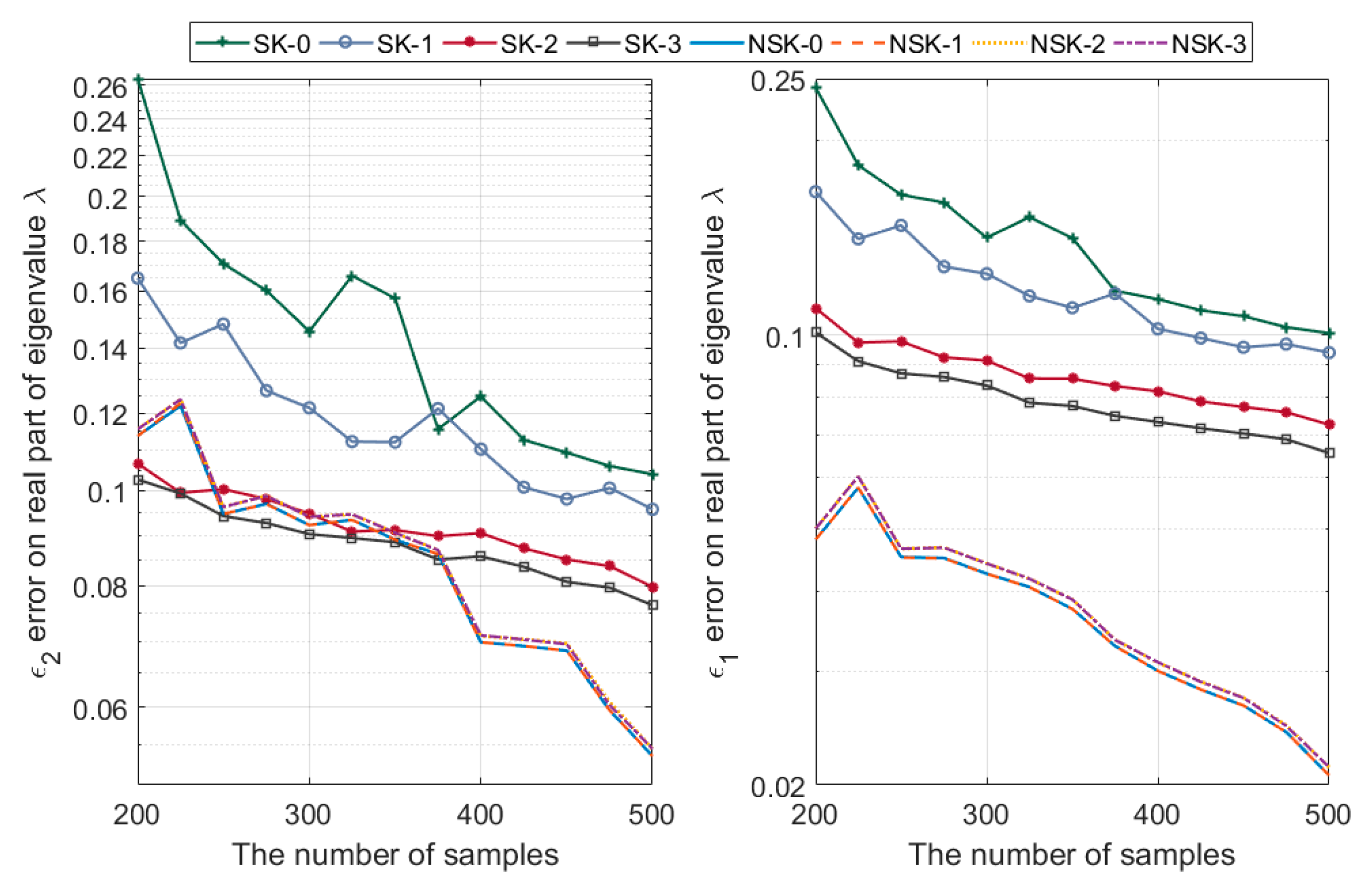
The reason for introducing Equation (23) is to compute the error due to the spurious oscillations more accurately. The 2-norm and 1-norm error for real eigenvalue pairs are presented in Figure 14. The abbreviation SK-i and NSK-i, denote stationary and nonstationary kriging with the i-th order polynomial trend function, respectively. The nonmonotonic convergence patterns, which are frequently observed in stationary kriging, are related to the optimization, sample sensitivities, and response complexity. In the case of nonstationary kriging, the classification of the given sample also affects the convergence behavior. However, the solution accuracy tends to improve as the number of samples increases. The results in Figure 14 indicate that nonstationary kriging shows better performance for all polynomial orders than stationary kriging. Although stationary kriging results are highly sensitive to the applied polynomial order, the nonstationary kriging results are less sensitive and yield similar errors for all considered polynomial orders. Comparing the 2-norm and 1-norm error, the error difference between stationary and nonstationary kriging is larger in the 1-norm based measure. This implies that the proposed method reflects the flattened region of response correctly, while stationary kriging reflects the stable region in an oscillated form.

4.3. Case 3: Study with a Random Friction Coefficient and Disc’s Material Properties

In the final case study, the friction coefficient, Young’s modulus and density of the disc are considered to be random. These properties are modeled using random variables as follows:

$$\begin{array}{ll}\mu & =0.5+0.5{\zeta }_1\\ E_{\mathrm{disc}}& =125\times {10}^9\left(1+0.2{\zeta }_2\right)\\ {\rho }_{\mathrm{disc}}& =7200\left(1+0.2{\zeta }_3\right)\end{array}$$

(24)

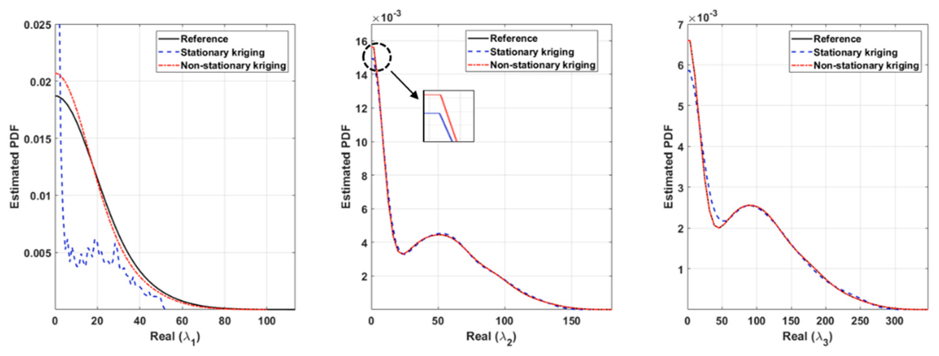
where ${\zeta }_1,{\zeta }_2$, and ${\zeta }_3$ are uniform random variables within the interval $\left[-1,1\right]$. By using 200 Sobol sequential samples, the stationary and nonstationary kriging with constant trend function are applied. The hyperplane results of the SVM for three unstable eigenvalue pairs are shown in Figure 15. Based on the obtained metamodels, probability density functions (PDF) for the real part of the three unstable eigenvalues are estimated; the results are presented in Figure 16. In obtaining the reference results, 10,000 samples using Latin hypercube sampling (LHS) are considered.

It can be seen from the stationary kriging results that for the first eigenvalue, the estimated PDF is inaccurate. Although the overall shape of the PDF for the second and third eigenvalues matches well with the reference results, the error still exists near the stable region (i.e., Real($\mathsf{\lambda }$) = 0). However, the proposed method yields almost identical results to the reference for the second and third eigenvalues, even in the stable region. For the first eigenvalue, although there is still an error, the proposed method shows better performance than stationary kriging.

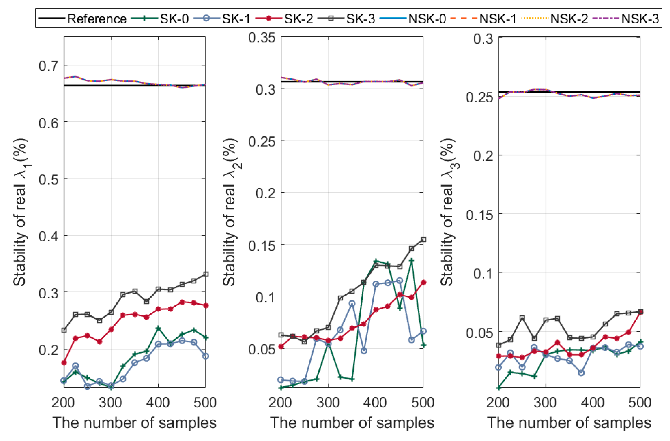
Next, to evaluate the metamodel performance, the Sobol sequential samplings, from 200 to 500 with increments of 25, are applied. Polynomial functions from 0th to 3rd order are considered as a trend function. The 2-norm and 1-norm error for the real part of eigenvalue pairs are presented in Figure 17. The obtained results indicate that for 2-norm-based error criteria, stationary and nonstationary kriging show similar performance in the small sample sizes. However, for 1-norm-based error criteria, nonstationary kriging outperforms over the stationary kriging within the all considered the sample sizes and polynomial orders. To further investigate the performance of the metamodels, the propensity of stability is considered. Given N samples, the i-th eigenvalue stability can be estimated as follows:

$$P_S^i=\mathrm{E}\left[I_{\mathsf{\Omega }}^i\left(\zeta \right)\right]\simeq \frac{1}{N}{\displaystyle \sum _{j=1}^N{I}_{\mathsf{\Omega }}^i\left({\zeta }^j\right)}=\frac{N_{\mathrm{stable}}^i}{N}$$

(25)

where $N_{\mathrm{stable}}^i$ is the number of stable samples for i-th eigenvalue, and $I_{\mathsf{\Omega }}^i\left(\zeta \right)$ is the indicator function given by

$$I_{\mathsf{\Omega }}^i\left(\zeta \right)=\{\begin{array}{cc}1,& {\lambda }_i\left(\zeta \right)<\mathrm{tol}\\ 0,& \mathrm{otherwise}\end{array}$$

(26)

where tol is the tolerance of the indicator function. Under 10,000 LHS samples and 0.1 tolerance, the reference eigenvalue stability in Equation (25) is computed. The propensity of stability based on the constructed metamodels is computed using the predicted responses at the LHS sample points. The obtained results for the three eigenvalues are presented in Figure 18. As seen from the results, although stationary kriging shows similar performance with nonstationary kriging based on 2-norm error criteria, their stability results are completely different. None of the stationary kriging results predict the stability of the response within the range of the given sample sizes, while nonstationary kriging yields similar results with the reference. The reason for this difference is that the oscillation phenomenon in stationary kriging is much larger than the tolerance of the indicator function in Equation (26). This implies that although the stationary kriging based metamodel seems to be applicable to the brake system in terms of 2-norm based error, it is difficult to investigate the propensity of the stability. However, in the case of nonstationary kriging, since spurious oscillation is alleviated by applying the step-wise hyperparameters, the obtained results are close to the reference.

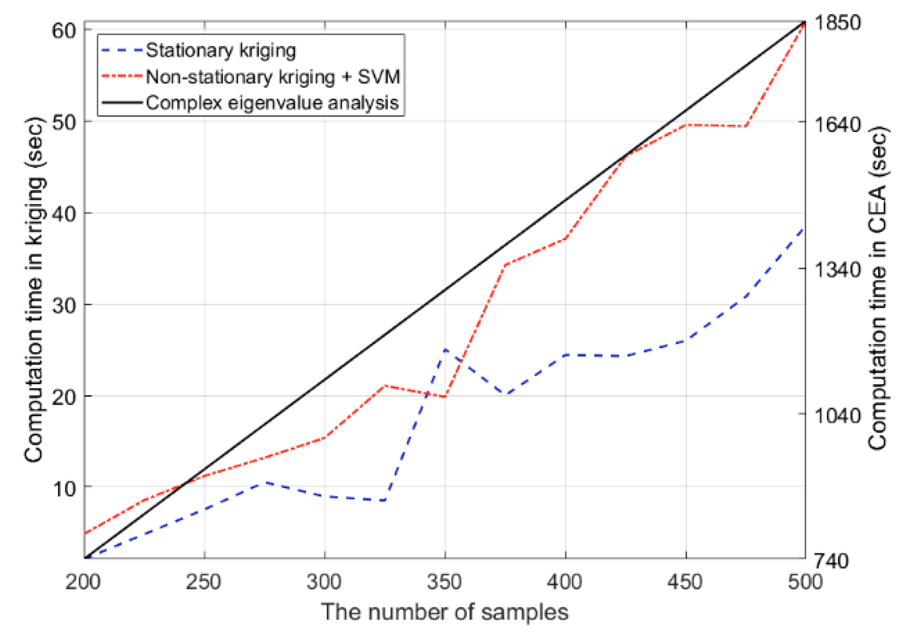
Finally, the computational cost and numerical efficiency of the proposed method are discussed. Given the finite element model, it takes about 3.7 s to solve the complex eigenvalue problem for one sample, and the total computation time is assumed to be linear for the given sample sizes. The total computation time results for complex eigenvalue problems, and stationary and nonstationary kriging, are given in Figure 19. The right and left y-axis are computation time in eigenvalue problems and kriging, respectively. The obtained results indicate that although the computation cost for nonstationary kriging is higher than that for stationary kriging, its additional cost can be relatively negligible when compared to solving the eigenvalue problems. Therefore, for the small number of random variables, the proposed nonstationary kriging can improve metamodel performance with acceptable additional computation.

5. Conclusions

In this study, a new combined nonstationary kriging and SVM is proposed to conduct stochastic eigenvalue analyses of brake systems. The proposed algorithm utilizes the nonstationary kernel reflecting the bifurcation region of the eigenvalue in the random input space. In order to divide the given samples into stable and unstable regions, a mode-coupling based stability criteria function is proposed. Finally, the support vector machine-based classification is applied to estimate the stability condition of the unsampled point, and the response is predicted.

To validate the performance of the proposed method, three stochastic eigenvalue problems in the simplified brake system are considered. The results applying the nonstationary kriging method are in good agreement with the reference, while the conventional stationary kriging shows oscillatory behavior and sample-sensitive results. Especially in predicting the propensity of stability, the proposed method outperforms the stationary kriging. This is attributed to the length scale with step-wise hyperparameters, which can represent nonstationary behavior. The additional computational cost for nonstationary kriging has been examined, and taking into account the cost for complex eigenvalue problems, it can be considered relatively negligible for the small number of random variables.

The obtained results indicate that the proposed method is promising for both accuracy and robustness, implying the possibility of its application to more complex brake system problems. In this paper, the stability criteria function is valid for only singular-coalescence point cases. Therefore, further research on various types of damping is necessary to generalize the proposed framework.

References

- Papinniemi, A.; Lai, J.C.; Zhao, J.; Loader, L. Brake squeal: A literature review. Appl. Acoust. 2002, 63, 391–400. [Google Scholar] [CrossRef]
- Sinou, J.-J.; Jézéquel, L. Mode coupling instability in friction-induced vibrations and its dependency on system parameters including damping. Eur. J. Mech.-A/Solids 2007, 26, 106–122. [Google Scholar] [CrossRef] [Green Version]
- Hoffmann, N.; Gaul, L. Effects of damping on mode-coupling instability in friction induced oscillations. ZAMM-J. Appl. Math. Mech./Z. Angew. Math. Mech. Appl. Math. Mech. 2003, 83, 524–534. [Google Scholar] [CrossRef]
- Hoffmann, N.; Fischer, M.; Allgaier, R.; Gaul, L. A minimal model for studying properties of the mode-coupling type instability in friction induced oscillations. Mech. Res. Commun. 2002, 29, 197–205. [Google Scholar] [CrossRef]
- Liu, P.; Zheng, H.; Cai, C.; Wang, Y.; Lu, C.; Ang, K.; Liu, G. Analysis of disc brake squeal using the complex eigenvalue method. Appl. Acoust. 2007, 68, 603–615. [Google Scholar] [CrossRef]
- AbuBakar, A.R.; Ouyang, H. A prediction methodology of disk brake squeal using complex eigenvalue analysis. Int. J. Veh. Des. 2008, 46, 416–435. [Google Scholar] [CrossRef]
- Chevennement-Roux, C.; Dreher, T.; Alliot, P.; Aubry, E.; Lainé, J.-P.; Jézéquel, L. Flexible wiper system dynamic instabilities: Modelling and experimental validation. Exp. Mech. 2007, 47, 201–210. [Google Scholar] [CrossRef]
- Culla, A.; Massi, F. Uncertainty model for contact instability prediction. J. Acoust. Soc. Am. 2009, 126, 1111–1119. [Google Scholar] [CrossRef] [PubMed]
- Nobari, A.; Ouyang, H.; Bannister, P. Statistics of complex eigenvalues in friction-induced vibration. J. Sound Vib. 2015, 338, 169–183. [Google Scholar] [CrossRef]
- Xiu, D.; Karniadakis, G.E. The wiener—Askey polynomial chaos for stochastic differential equations. SIAM J. Sci. Comput. 2002, 24, 619–644. [Google Scholar] [CrossRef]
- Krige, D.G. A statistical approach to some basic mine valuation problems on the Witwatersrand. J. S. Afr. Inst. Min. Metall. 1951, 52, 119–139. [Google Scholar]
- Nechak, L.; Berger, S.; Aubry, E. A polynomial chaos approach to the robust analysis of the dynamic behaviour of friction systems. Eur. J. Mech.-A/Solids 2011, 30, 594–607. [Google Scholar] [CrossRef] [Green Version]
- Zhang, Z.; Oberst, S.; Lai, J.C. On the potential of uncertainty analysis for prediction of brake squeal propensity. J. Sound Vib. 2016, 377, 123–132. [Google Scholar] [CrossRef]
- Denimal, E.; Nechak, L.; Sinou, J.-J.; Nacivet, S. Kriging surrogate models for predicting the complex eigenvalues of mechanical systems subjected to friction-induced vibration. Shock Vib. 2016, 2016. [Google Scholar] [CrossRef] [Green Version]
- Nechak, L.; Gillot, F.; Besset, S.; Sinou, J.-J. Sensitivity analysis and Kriging based models for robust stability analysis of brake systems. Mech. Res. Commun. 2015, 69, 136–145. [Google Scholar] [CrossRef]
- Sarrouy, E.; Dessombz, O.; Sinou, J.-J. Piecewise polynomial chaos expansion with an application to brake squeal of a linear brake system. J. Sound Vib. 2013, 332, 577–594. [Google Scholar] [CrossRef] [Green Version]
- Nechak, L.; Besset, S.; Sinou, J.-J. Robustness of stochastic expansions for the stability of uncertain nonlinear dynamical systems–application to brake squeal. Mech. Syst. Signal Process. 2018, 111, 194–209. [Google Scholar] [CrossRef]
- Fischer, K.; Wriggers, P. Frictionless 2D contact formulations for finite deformations based on the mortar method. Comput. Mech. 2005, 36, 226–244. [Google Scholar] [CrossRef]
- Wriggers, P.; Zavarise, G. Computational Contact Mechanics; John Wiley & Sons, Ltd.: Hoboken, NJ, USA, 2004. [Google Scholar]
- Ghanem, R.G.; Spanos, P.D. Stochastic Finite Elements: A Spectral Approach; Courier Corporation: North Chelmsford, MA, USA, 2003. [Google Scholar]
- Gibbs, M.N. Bayesian Gaussian Processes for Regression and Classification. Ph.D. Thesis, University of Cambridge, Cambridge, UK, 1998. [Google Scholar]
- Martin, J.D.; Simpson, T.W. Use of kriging models to approximate deterministic computer models. AIAA J. 2005, 43, 853–863. [Google Scholar] [CrossRef]
- Cristianini, N.; Shawe-Taylor, J. An Introduction to Support Vector Machines and Other Kernel-Based Learning Methods; Cambridge University Press: Cambridge, UK, 2000. [Google Scholar]
- Marelli, S.; Sudret, B. UQLab: A framework for uncertainty quantification in Matlab. In Vulnerability, Uncertainty, and Risk: Quantification, Mitigation, and Management; American Society of Civil Engineers: Reston, VA, USA, 2014; pp. 2554–2563. [Google Scholar]