Statistical Process Control with Intelligence Based on the Deep Learning Model


Beijing Key Laboratory of Advanced Manufacturing Technology, Beijing University of Technology, Beijing 100124, China
*
Author to whom correspondence should be addressed.
Appl. Sci. 2020, 10(1), 308; https://doi.org/10.3390/app10010308
Submission received: 5 December 2019
/
Revised: 24 December 2019
/
Accepted: 30 December 2019
/
Published: 31 December 2019
(This article belongs to the Special Issue Novel Industry 4.0 Technologies and Applications)
Abstract
:Statistical process control (SPC) is an important tool of enterprise quality management. It can scientifically distinguish the abnormal fluctuations of product quality. Therefore, intelligent and efficient SPC is of great significance to the manufacturing industry, especially in the context of industry 4.0. The intelligence of SPC is embodied in the realization of histogram pattern recognition (HPR) and control chart pattern recognition (CCPR). In view of the lack of HPR research and the complexity and low efficiency of the manual feature of control chart pattern, an intelligent SPC method based on feature learning is proposed. This method uses multilayer bidirectional long short-term memory network (Bi-LSTM) to learn the best features from the raw data, and it is universal to HPR and CCPR. Firstly, the training and test data sets are generated by Monte Carlo simulation algorithm. There are seven histogram patterns (HPs) and nine control chart patterns (CCPs). Then, the network structure parameters and training parameters are optimized to obtain the best training effect. Finally, the proposed method is compared with traditional methods and other deep learning methods. The results show that the quality of extracted features by multilayer Bi-LSTM is the highest. It has obvious advantages over other methods in recognition accuracy, despite the HPR or CCPR. In addition, the abnormal patterns of data in actual production can be effectively identified.
1. Introduction
Since 1920s, statistical process control (SPC) theory has played an important role in product quality improvement and quality supervision [1]. SPC mainly uses a statistical analysis method to monitor the production process, and scientifically distinguishes the random fluctuation and abnormal fluctuation of product quality in the production process [2,3]. Thus, the abnormal trend of production process is expected, so that production managers can take timely measures to eliminate abnormalities and restore the stability of the process, so as to achieve the purpose of improving and controlling the quality. Intelligent SPC data analysis is realized, which can reduce production time and cost and improve product quality. It will likely become an integral part of industry 4.0 technology. Among the many theories of SPC, control charts and histograms are the most important and practical visual indicators [4]. If the manufacturing process is affected not only by random factors, but also by other specific factors, there will be specific abnormal patterns in the control chart and histogram [5]. For example, as far as the control chart is concerned, the cyclic patterns might be related to the periodic variation in the power supply. Trend patterns may be related to factors that change slowly, while changes in raw materials, workers and machine tools may cause shift patterns.
In the early application of control charts, it is necessary to manually determine whether or not there is any abnor–mality in the control charts and what kind of abnormality occurs. It is easy to detect abnormalities beyond the control limit, but difficult to identify abnormal patterns within the control limit, which is easily affected by the experience level of quality control personnel [6]. Then, many non-natural pattern detection methods based on supplementary rules were proposed by scholars [7,8,9]. The Nelson criterion is one of these methods [10]. However, control charts contain a lot of information about the production process. Supplementary rules cannot describe the specific modes of a process in detail. In addition, a large number of rules are used, which is not conducive to the real-time monitoring of production process, and will cause many false alarms [11,12]. In order to realize automated control chart pattern recognition (CCPR), scholars have designed a series of expert systems so that quality management personnel can take timely remedial measures for uncontrolled manufacturing process [13,14,15,16]. They are mainly based on statistical tests and heuristic algorithms [17]. Because of the shortcomings of these judgment rules, early expert systems cannot get satisfactory results [18]. This stimulates interest in developing more accurate CCPR algorithms.
Because machine learning algorithms have strong pattern recognition capabilities, their applications in the CCPR field have received more and more attention and achieved some success. It mainly includes an artificial neural network (ANN) and a support vector machine (SVM). The multilayer perceptron (MLP) are the most widely used in ANN-based methods [19,20,21]. In [22], an effective CCPR system based on MLP is studied. The effects of different layers of MLP and different training algorithms on the results are also compared. It is found that the resilient back-propagation (RBP) algorithm has the best convergence speed and the Levenberg–Marquardt (LM) algorithm has the best optimization effect. In [23], a new learning algorithm based on bees algorithm is adopted, and an optimized radial basis function neural network (RBFNN) is trained, which shows good performance in CCPR tasks. In addition, the probability neural network (PNN) [24], spiking neural network (SNN) [25] and learning vector quantization (LVQ) [26,27,28] are also widely used. They all belong to supervised learning algorithms. At the same time, unsupervised algorithms such as self-organizing mapping (SOM) [29] and adaptive resonance theory (ART) are also used in CCPR. Because of its shallow structure and limited learning ability, ANN has some shortcomings, such as difficulty in convergence and can easily fall into local minimum, which limits its further development. Subsequently, SVM and its variants have been proposed by scholars and used to solve CCPR problems. For example, weighted SVM [30], multi-kernel SVM [31] and fuzzy SVM [1]. They generally show better recognition accuracy than traditional ANN.
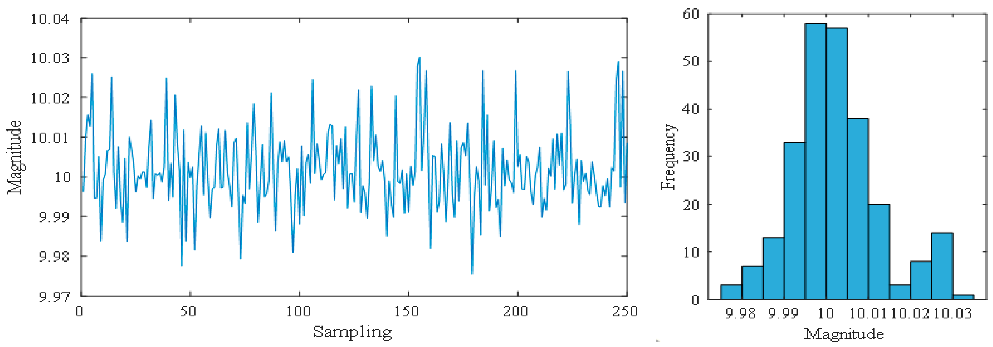
Histogram is a graphical representation of the distribution of quality data. Its distribution degree is a common tool for judging and predicting the quality of production process. Similar to the control chart pattern (CCP), the abnormality of the histogram pattern (HP) corresponds to specific factors. For example, skewed patterns are caused by poor processing habits of workers, and flat-top patterns indicate that production processes are affected by slow-changing factors. As far as we know, only one paper has studied histogram pattern recognition (HPR) in SCI and EI database in recent years [4]. In [4], an HPR method based on a fuzzy ART neural network is proposed. The advantage of this method is that it can cluster HPs adaptively and generate new classes for unknown patterns. At the same time, there is a big risk to classify the known patterns into new categories, which is not conducive to practical application. Moreover, the simulation data used in this paper are not random enough. The quality data of real processes cannot be fully simulated. The lack of research on HPR is a major drawback of SPC intelligent research. This is because histograms and control charts complement each other, as shown in Figure 1. According to the theory of a control chart, the quality data is normal. However, its histogram pattern is an island pattern, which means that the production process is abnormal. Control charts are suitable for identifying short-term anomalies, while histograms can reflect the long-term distribution of quality data. Therefore, the role of a histogram cannot be ignored, and enterprises are also in urgent need of accurate automatic HPR.
It is well known that in the field of pattern recognition, the input form of data has a great influence on classification, which is called the input representation problem. One form is to take the raw data as input [24,32,33], such as quality data in the control chart and the frequency of each interval in the histogram. Another form is to take the features extracted from the raw data as input, such as wavelet features [11], shape features [19,34,35] and statistical features [23,34]. The latter is called feature engineering, that is, experts design favorable features for pattern recognition problems based on experience. Most scholars’ research shows that if the dimension of input data is too large, the classifier size of traditional machine learning algorithm will be too large, which is unfavorable. Its accuracy and efficiency are often lower than the feature-based method, because the dimension of feature set is usually very small [11,29]. There is no doubt that the key to improve classification accuracy is to select the most advantageous feature set. To achieve this goal, a genetic algorithm (GA) [1] and local linear embedding (LLE) [36] are used to optimize features from high-dimensional feature sets. However, they only select good features from the known expert feature set, and do not improve the quality of feature set from the root. The discarded raw data still has potential values, so more advanced methods, such as feature learning, still need to be used. Feature learning refers to adaptively extract the most advantageous features from the raw data by using the deep neural network (DNN), without relying on any expert experience. Since the feature set is obtained by learning and minimizing the loss function, it can be considered that this feature set is the best choice for this classification task [37]. The most representative deep learning algorithms include the deep belief network (DBN) [38,39] based on the restricted Boltzmann machine (RBM), the convolutional neural network (CNN) [40,41,42] based on the convolution layer and pooling layer and the recurrent neural network (RNN) [43,44] based on the recursive layer. They have made remarkable achievements in machine vision, natural language processing and fault diagnosis [45].
On the basis of relevant research in recent years [18,46,47], this paper proposes to use multilayer bidirectional long short-term memory networks (Bi-LSTM) to learn the features of histogram and control chart, and finally realize HPR and CCPR. The Bi-LSTM is an improved method of RNN. Its special gate structure enables it to capture both short-term dependencies and long-term dependencies. This paper is an extension of previous studies [18]. Different from previous studies, multilayer Bi-LSTM is used to replace the former one-dimensional CNN (1D-CNN), because it is specially used to process one-dimensional data such as time series, and has a stronger ability to process the relationship between before and after the sequence. It has also been compared with the traditional method and many typical deep learning methods. In addition, besides automatic CCPR, accurate HPR is also realized. Until now, HPR has been ignored by scholars. In this way, the automation and intelligence level of SPC has been improved more comprehensively. Furthermore, the six CCPs were studied before they were expanded to nine, making the CCPR more comprehensive and refined. In order to detect anomalies in production as quickly as possible, the length of the data we use for pattern recognition is 25. This is because longer data may mean that more defective products have been produced in the factory when abnormalities are identified [18].
The rest of this paper is organized as follows. Section 2 explains the basic structure of LSTM and the mathematical representation of HPs and CCPs. Section 3 introduces the details and process of the proposed method. Section 4 carries on the experiment and completes the related discussion. Finally, Section 5 summarizes the paper and gives the prospect of future work.
2. Methodology
2.1. Simulation Method of Histogram Patterns
Seven typical HPs of the production process are shown in Figure 2, including normal (NOR) patterns, bimodal (BIM) patterns, left and right island (LI and RI) patterns, left and right skew (LS and RS) patterns and flat top (FT) patterns.
The Monte Carlo simulation algorithm is recognized as a HP simulation method in the SPC field [48]. In this paper, the method is used to simulate the quality data of each HP.
If is the value of quality data measured at , then the quality data in the NOR pattern is normal distribution:
where is the mean of quality data under controlled conditions, is the standard deviation.
The quality data of BIM pattern is a combination of two normal distributions, which can be simulated by the following formula [48]:
where, and are the proportion of two normal distributions, and and are the distance between the center of two normal distributions and .
The LI and RI pattern can be seen as a small normal distribution next to the normal distribution., which can be simulated by the following formula:
where, and are the proportion of two normal distributions, and is the distance between the center of small normal distributions and ; “+” represents RI pattern, and “−” represents LI pattern.
The quality data of LS and RS pattern can be combined by several normal distributions [48], which can be simulated by the following formula [48]:
where, is the number of normal distributions; “+” represents LS pattern, and “−” represents RS pattern.
FT pattern quality data can be formed by mixing uniform distribution with normal distribution, which can be simulated by the following formula:
where, and are the proportion of normal distribution and uniform distribution respectively.
2.2. Simulation Method of Control Chart Patterns
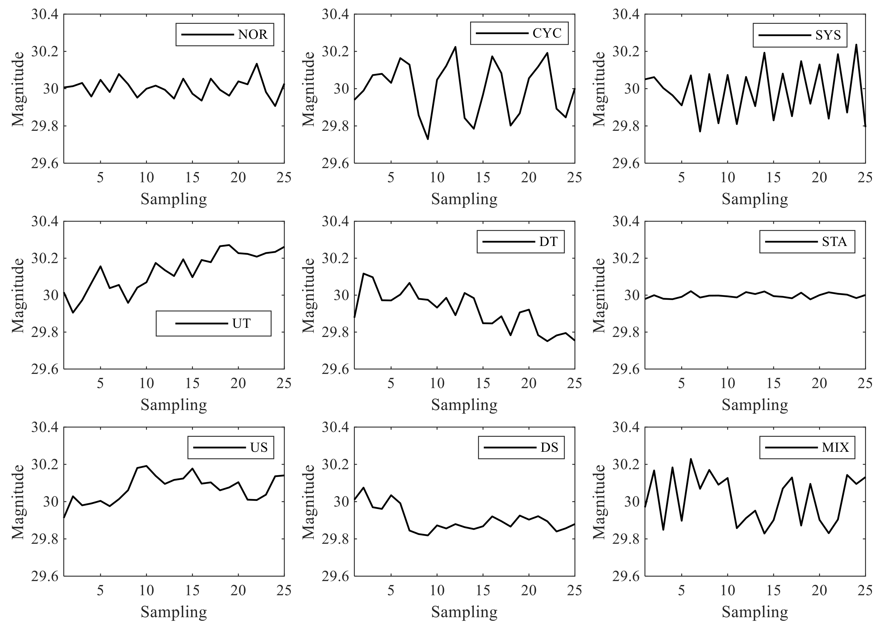
Nine typical CCPs of the production process are shown in Figure 3, including normal (NOR) patterns, cycle (CYC) patterns, systematic (SYS) patterns, upward and downward trend (UT and DT) patterns, stratification (STA) patterns, upward and downward shift (US and DS) patterns and mixture (MIX) patterns.
Equation (6) is a general formula for simulating various CCP, which includes the process mean and two noise components [5]: is random noise and is a special fluctuations from specific factors in manufacturing process.
where is the quality data at time t. μ is the mean value of the product. Random noise obeys normal distribution, .
A detailed description of the simulation methods of nine typical CCPs can be found in Section 4.6 or [49]. We will not repeat the description here.
2.3. Long Short-Term Memory Network Model
In recent years, deep learning has made remarkable achievements in various fields. The deep learning algorithm has advantages that the traditional shallow machine learning algorithm does not have, such as complex data preprocessing and feature engineering are no longer needed. The raw data can be used as the input of the model. The deep-seated of neural network and the special design of network structure make it can learn the potential deeper knowledge from the raw data and be competent for more complex tasks. The features it learns are the most suitable for this classification task and fares better than the features designed by human experts.
LSTM is a typical deep learning model and a variant of RNN. The basic idea is still to take the previous output of the network as the next input, as shown in Equation (7). Where is the input of the network, h is the output of the network, and H is the nonlinear transformation function.
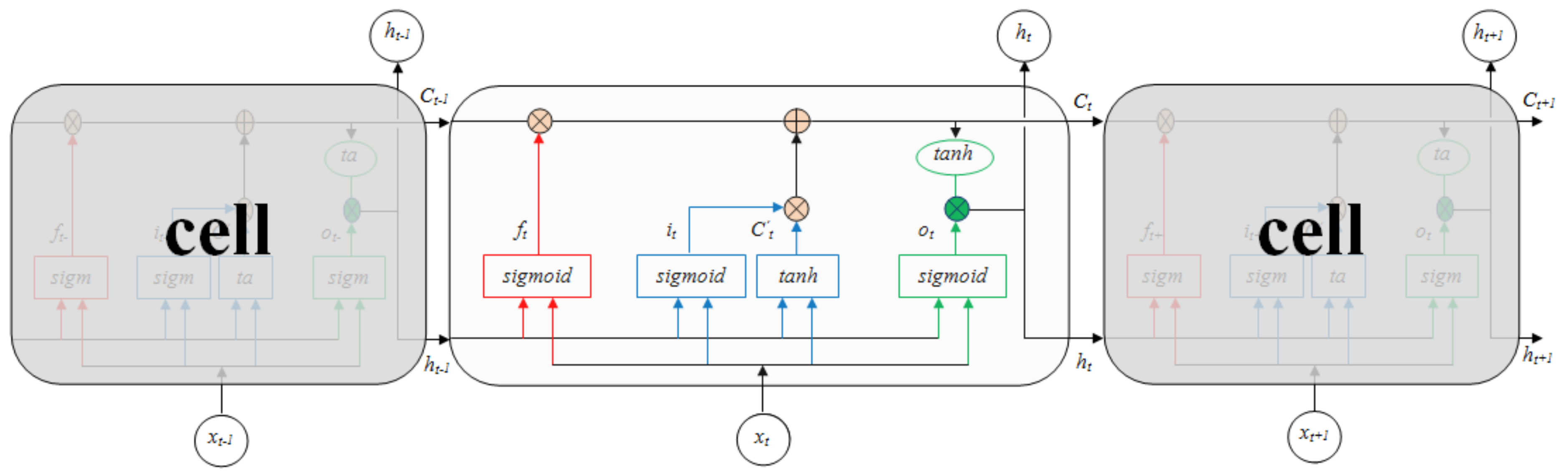
Compared with traditional RNN, LSTM can capture long-distance dependency. It is different from the standard RNN in structure. LSTM adds some gate structures for each cell, which allows information to pass selectively. It can be understood as a mechanism of feature learning selection and update [45]. The cell structure of LSTM is shown in Figure 4.
The forget gate (the red part in Figure 4) is used to decide what information will be discarded from the cell state . A forget gate is mathematically represented by [45]:
The input gate (the blue part in Figure 4) is used to determine what new information will be stored in the cell state. A input gate is mathematically represented by [45]:
Then the cell state is updated, and the decisions made in the previous steps are implemented to get a new cell state . The mathematical representation of the state update is as follows:
The output gate (the green part in Figure 4) determines the final output according to the updated cell state. An output gate is mathematically represented by [45]:
where , , and represent the weight of forget gate, input gate, current cell and output gate respectively. , , and represent the bias.
The final output of the last cell of LSTM is the feature extracted adaptively from the raw data (where refers to the last cell). The final recognition can be achieved by inputting this feature into the traditional ANN. The last layer is the output layer, whose activation function is Softmax, and the number of neurons is N, representing the number of types that want to identify patterns. Finally, the stochastic gradient descent (SGD) algorithm is used to optimize the weight (, , and ) and bias (, , and ) in LSTM. Commonly used SGD methods include SGD with momentum (SGDM), root mean square propagation (RMSProp), and adaptive moment estimation (Adam) [50].
In this paper, Bi-LSTM is used to complete CCPR and HPR, which is slightly different from standard LSTM, that is, Bi-LSTM consists of forward LSTM and backward LSTM. More details of the Bi-LSTM structure are introduced in the following sections.
3. Proposed Method
This section describes the details of the proposed method. The input of the LSTM is the unprocessed data, such as quality data in the control chart and the frequency of each interval in the histogram, and the output is the category of the pattern. Feature extraction, and feature selection are all completed by LSTM through learning. Compared with unidirectional LSTM, Bi-LSTM can learn the front and back relation of sequence better.
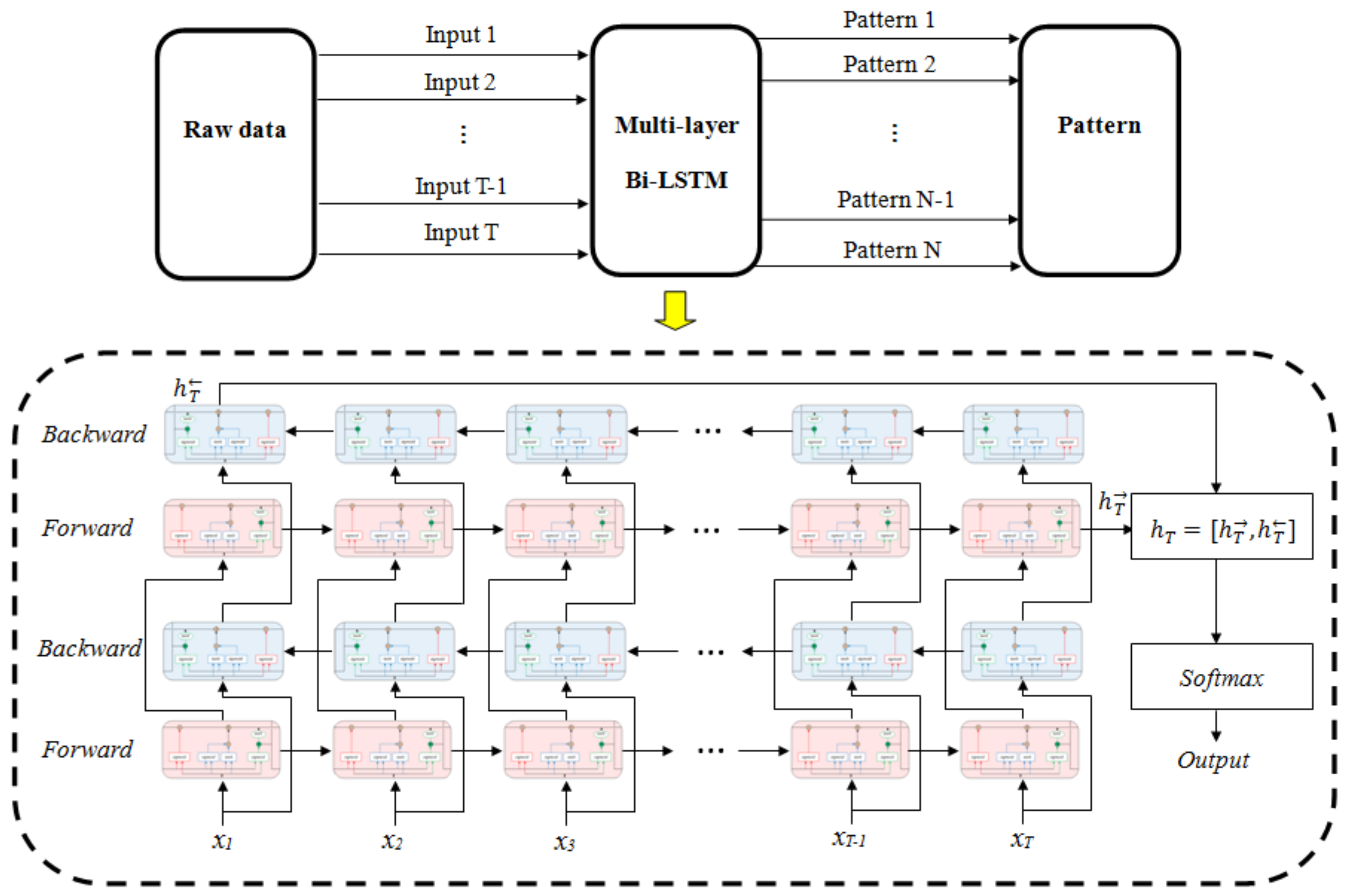
Figure 5 is a structural diagram of the proposed method. It has a bidirectional recursive layer as well as a multilayer structure. When the input of the model passes through a multilayer structure, the information transmitted by each layer will be represented in different dimension spaces. Therefore, data is gradually learned by increasing the number of layers of the network. The connection between input and output is improved to better describe the characteristics of the system [51]. In other words, bidirectional and multilayer recursive structure can raise the learning space and flexibility of the model [45]. Each small square in Figure 5 represents a LSTM cell.
The network consists of multilayer Bi-LSTM and a Softmax classifier. The former is used to extract features from the raw data, and the latter is used to classify various patterns. The input of Softmax layer is the combination of the last forward LSTM output and the last backward LSTM output , as shown in Equation (14). The initial learning rate was 0.05, and each LSTM cell has 10 neurons. The next section discusses and optimizes other structural and training parameters of multilayer Bi-LSTM, such as optimization algorithm, training batch size and network layer number.
Because of the end-to-end ability of deep learning method, the specific implementation process of the method proposed in this paper is as follows. Firstly, the Monte Carlo algorithm is used to simulate training set and test set of HPR and CCPR respectively. The one-hot encoding method is used to label the samples. Then, training sets are used to train two Bi-LSTMs, which are used for HPR and CCPR respectively. Finally, the performance of the optimized two Bi-LSTMs are verified by the test set and real production data.
4. Experiment and Discussion
In this section, some simulation data experiments and production data experiments were used to verify superiority of the multilayer Bi-LSTM. It was implemented by the MATLAB environment, and the experiment was carried out on a 3.10 GHz CPU with 4 GB RAM. The correct recognition rate (CRR) was used as the evaluation standard of model performance. At the same time, the discussion related to the experiment results was completed.
4.1. Simulation Parameters of HPs
In order to make the simulation data closer to the complex production data, the Monte Carlo simulation parameters of the seven HPs were randomly selected within a certain range, using the uniform distribution. The range of parameters is shown in Table 1. For example, parameter a of all BIM pattern samples is uniform distribution in the range .
It is worth noting that the simulation results are the quality data of each HP, not the histogram. After that, interval statistics is needed to get histogram. The purpose of this simulation method is to be more in line with the actual situation. The quality data length of each sample is 500, and the number of groups of histogram is 25. The data set consists of 14,000 samples (2000 for each HP), which are randomly divided into two parts, of which 80% samples were used to train Bi-LSTM, and the rest was used for testing.
4.2. Performance Comparison of Optimization Algorithm
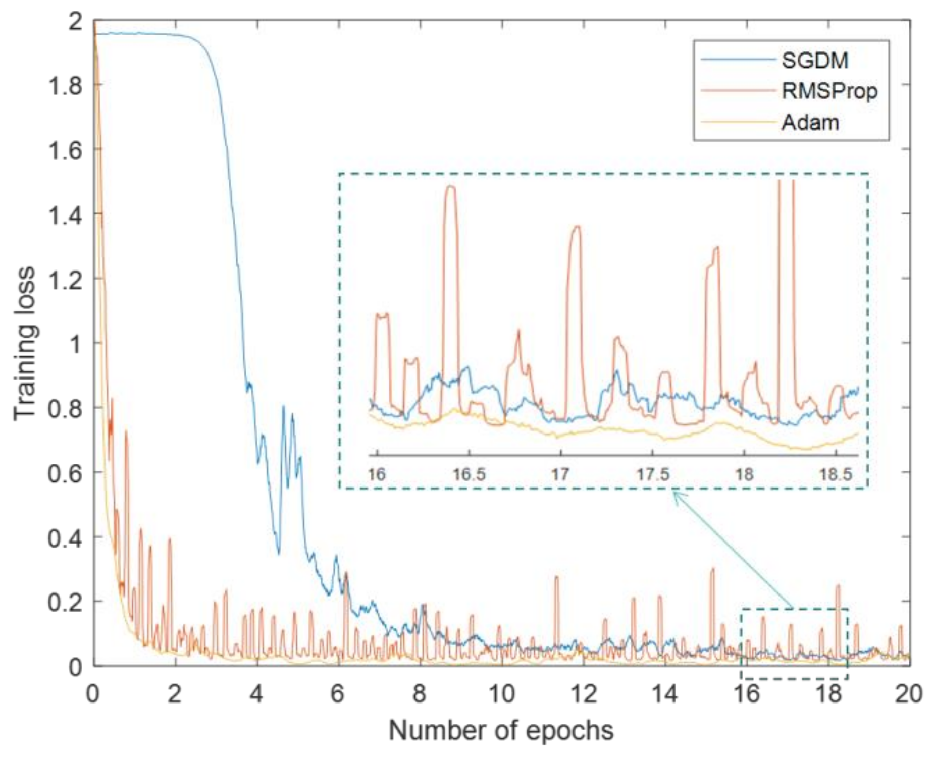
The SGD algorithm is a common optimization algorithm, which is often used to optimize the weight and bias of neural network in the training stage. However, the performance of its sub algorithm and variant is different. For this reason, in order to obtain the best training results, we compared several popular optimization algorithms, namely SGDM, RMSProp, and Adam [50]. Different optimization algorithms are used to train the Bi-LSTM. In this experiment, the training data set generated in Section 4.1 is used to complete the training. The initial learning rate is 0.05, and the batch size is 100. They were trained for 20 epochs and collected the corresponding training losses. The results are shown in Figure 6.
It can be seen from Figure 6 that the SGDM algorithm has a slow convergence speed, and has a large training loss. The convergence speed of the RMSProp algorithm is fast, but the training process fluctuates greatly, and the training loss is not ideal. The Adam algorithm has the fastest convergence speed, the smallest loss, and the process is stable. Therefore, this optimization algorithm with the best performance is applied in the following experiments.
SGDM algorithm uses a single learning rate in the whole training process. Other optimization algorithms use different learning rates to improve the network training, and can automatically adapt to the loss function being optimized. This is how the RMSProp algorithm works. Adam updates with parameters similar to RMSProp, but adds a momentum term to that [50]. Therefore, the neural network can obtain fast and stable training effect.
4.3. The Influence of Batch Size on Training Process
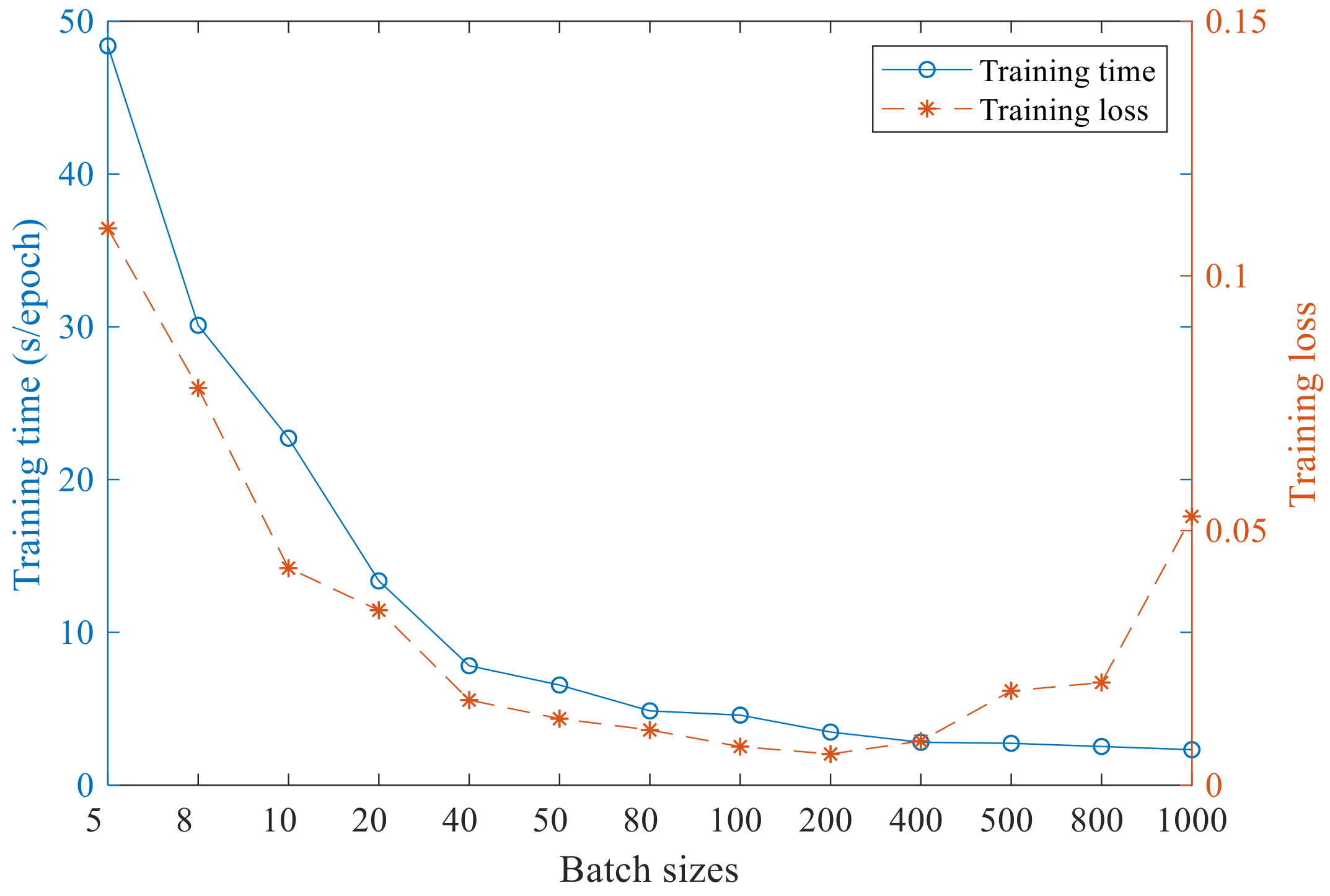
The batch size determines the number of samples for network learning in each iteration., it is an important part of network training parameters. According to the past experience, this parameter has great influence on the training result and training time. Therefore, in the experiment, different batch sizes were compared and the results are shown in Figure 7.
It can be seen from Figure 7 with the increase of batch size, the training time of each epoch decreases continuously, and tends to be stable when the batch size exceeds 200. However, with the increase of the batch size, the training loss first decreases and then increases, and it is the best when the batch size is 200. Therefore, when the batch size is 200, the recognition accuracy of Bi-LSTM can be guaranteed and the training time can be greatly reduced.
4.4. The Influence of the Number of Network Layers
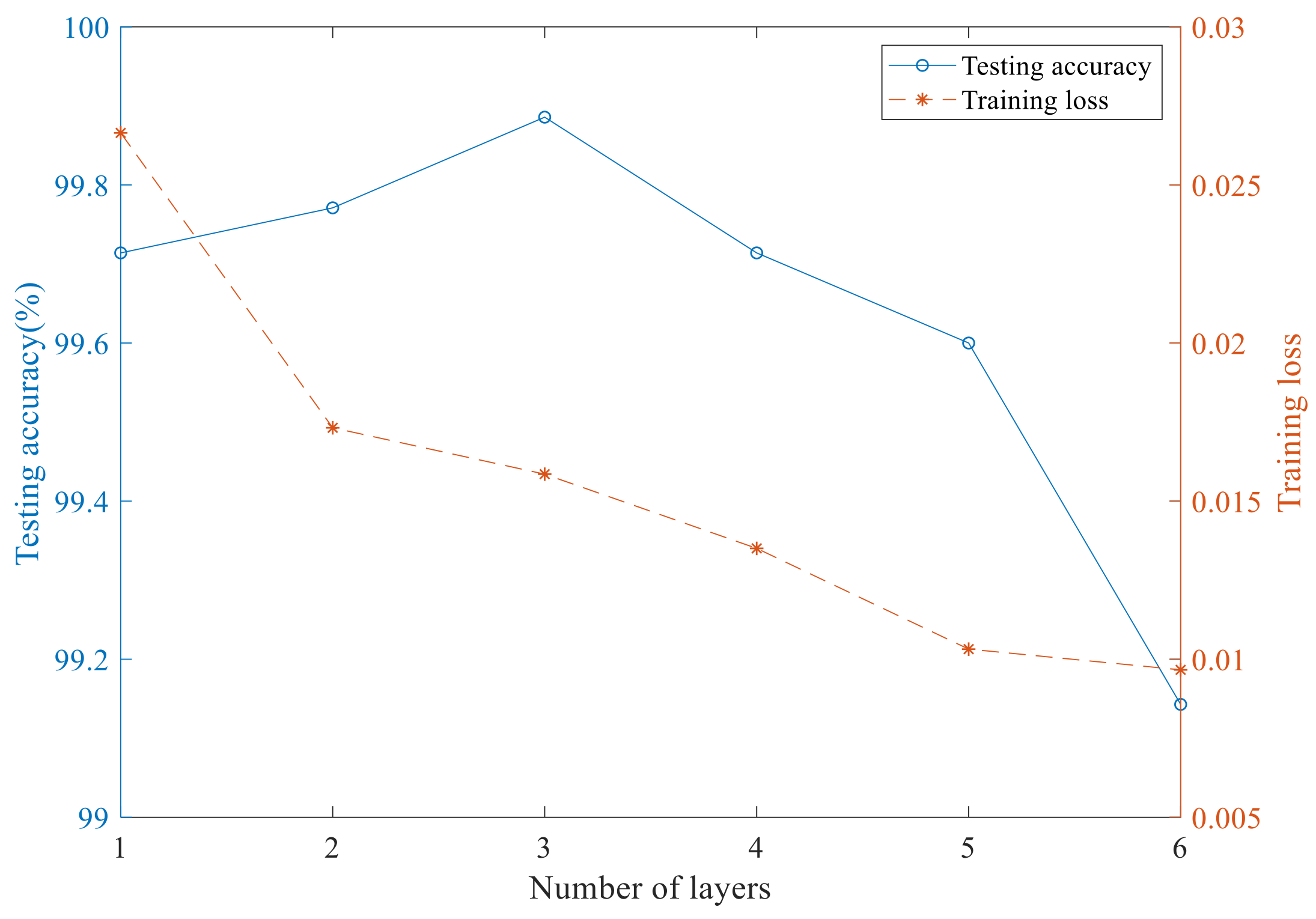
In the field of deep learning, this view is recognized by scholars. With the deepening of the network, the performance of it will be improved. This is because multilayer structure can improve the capacity and flexibility of the model [45]. However, some scholars a point out that the increase of network layers will increase the risk of over-fitting [51]. Therefore, this experiment compares the influence of the number of different network layers on training loss and testing accuracy, as shown in Figure 8. In this experiment, the network structure of Figure 5 is used, that is, the output of the first forward layer of the network is the input of the second forward layer, and the output of the first backward layer is the input of the second backward layer. According to this stacking rule, a multilayer network is formed. The data and training parameters used are the same as the above experiments. The training loss and testing accuracy of different networks are collected.
It can be seen from Figure 8, with the increase of the number of layers of the Bi-LSTM network, the training loss of the training set data continues to decrease, which shows that the network fits these training data better and better. On the contrary, the recognition rate of the trained multilayer Bi-LSTM network to the data of the test set increases first and then decreases. This is a typical over fitting phenomenon, that is, with the increase of the number of layers, the network continues to deepen, the fitting degree of the training set data is too high, and the generalization ability of the test set data is reduced. According to the above experimental results, it is finally determined that the number of layers of multilayer Bi-LSTM is 3.
4.5. Comparison of HPR Results of Several Methods
Through the above comparison experiments, the structural parameters and training parameters finally determined for multilayer Bi-LSTM are shown in Table 2.
In order to further verify the effectiveness of the proposed method in HPR tasks, we compare multilayer Bi-LSTM with traditional machine learning methods (MLP) and several deep learning methods (DBN and 1D-CNN). These methods are described in detail as follows:
- (1)
- MLP: There are three layers of MLP used in the experiment. The first layer of MLP is the input layer with 25 neurons, which are used to receive the frequency of 25 intervals of histogram. The second layer is the hidden layer with 30 neurons. The last layer is the output layer with seven neurons, corresponding to seven typical HPs. The activation function of all layers of MLP is Sigmoid function.
- (2)
- DBN: The input of DBN is the frequency of 25 intervals of histogram. The DBN in this experiment is composed of three layers of RBM. Each RBM layer is pre-trained unsupervised. After the layer by layer pre-training is completed, the supervised global optimization is carried out. Each RBM layer contains 60 neurons, and the activation function of all layers is the Sigmoid function.
- (3)
- 1D-CNN: The 1D-CNN used in this experiment is the structure recommended in [18]. The input of 1D-CNN is the frequency of 25 intervals of histogram. It consists of two convolution layers, two pooling layers and a full connection layer, and they are all one-dimensional. The number of feature maps of the two convolution layers is 6 and 12 respectively, and the convolution kernel size is 2*1 and 9*1, respectively. The activation function of the convolution layer was the rectified linear units (ReLU) function, and the output layer was the Softmax function.
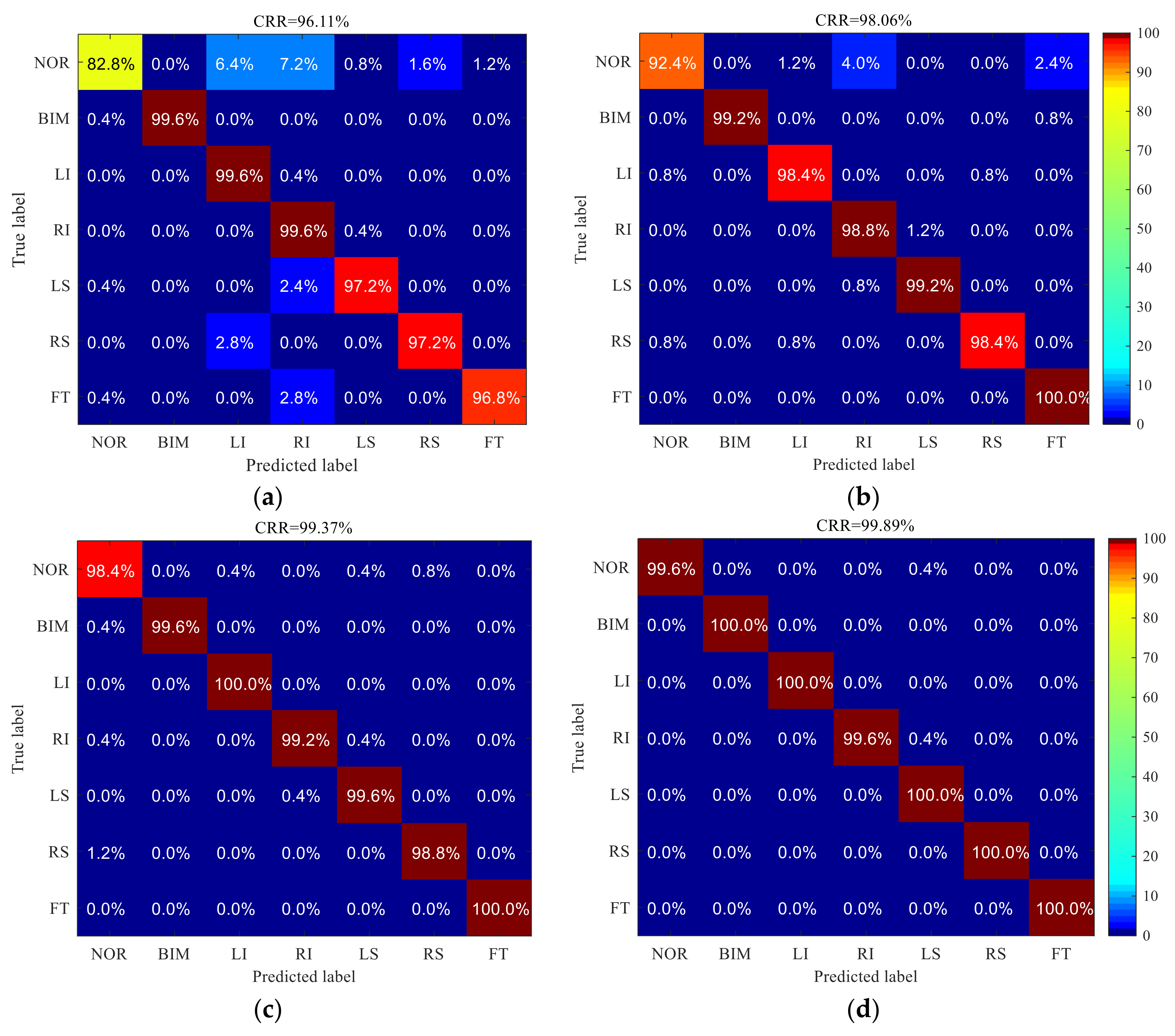
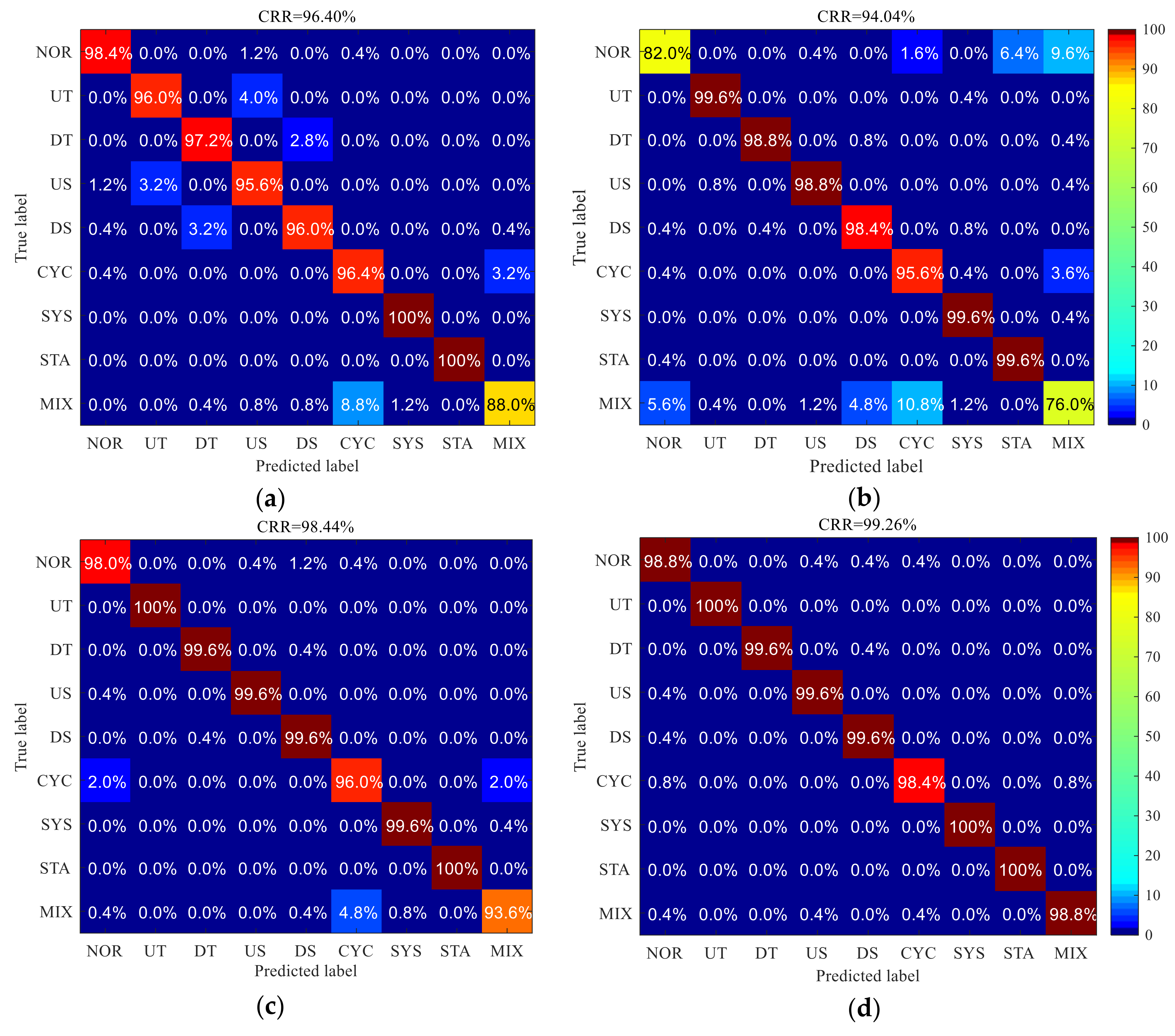
In order to observe the results of pattern recognition more intuitively, confusion matrix is used. The values of the elements on the diagonal of the confusion matrix respectively represent the proportion of the correct recognition of various patterns. Other values represent the misjudgment of the classifier. The total CRR is equal to the average of all elements on the diagonal [1]. The confusion matrix of various identification methods is shown in Figure 9, and the total CRR and the time consumption of each epoch in the training process are shown in Table 3.
Figure 9 shows that there are different levels of confusion in the recognition results of several HPR methods. However, the performance of three recognition methods based on deep learning is better than that of traditional machine learning methods. In the recognition results of several methods, there is a trend of confusion from the NOR pattern to the island pattern. This problem is the most serious in MLP method, followed by DBN method. This may be due to the similarity between the NOR pattern and the island pattern. This is an unacceptable result, which means that the HPR system based on these methods will have a very serious Type I error (false alarm), which will bring unnecessary trouble to the quality control work of the enterprise. On the contrary, the method based on 1-DCNN effectively improves the recognition results of nor pattern, and proves the effectiveness of processing one-dimensional data and the ability to capture the details of data. Due to the multilayer and bidirectional structure, the training time of multilayer Bi-LSTM is a little longer, but it gets a very satisfactory recognition result. In 2800 test samples, only 4 samples are misclassified, and the CRR is as high as 99.89%, achieving accurate HPR. Compared with other methods, it has obvious advantages.
4.6. Simulation Parameters of CCPs
The simulation parameters of nine common CCPs are shown in Table 4.
For the MIX pattern, p is a binary integer, which is randomly selected from 0 or 1 at each sampling time t in the sample. The value of v is determined by where the mutation occurs. It is equal to 0 before the mutation occurs and 1 after the mutation occurs. The starting position obeys uniform distribution in the range [4,9]. The quality data length of each CCP is 25. The data set consists of 18,000 samples (2000 for each CCP), which are randomly divided into two parts, of which 80% samples were used to train multilayer Bi-LSTM, and the rest was used for testing.
4.7. Comparison of CCPR Results of Several Methods
In order to further verify the effectiveness of the proposed method in CCPR tasks, we compare multilayer Bi-LSTM with traditional machine learning methods (MLP) and several deep learning methods (DBN and 1D-CNN). Among them, MLP is widely used in CCPR field [19,21,22], which is the reason why we compare with it in this paper. The network structure of these methods is exactly the same as was used in Section 4.5. The difference is the input of the network.
The input of MLP becomes CCP feature set, which includes statistical features (mean, standard deviation, skewness and kurtosis) and shape features (S, NC1, NC2, APML and APSL). These features are designed by experts in this field, and have been proved to be very effective in many years of application [18,19,33,34,35]. Therefore, the first input layer of MLP has nine neurons, which are used to receive the above nine features respectively. However, the input of the three methods based on deep learning is still the raw data, that is, the quality data on the control chart. This is because they can adaptively extract the best features from the raw data. The results are shown in Figure 10 and Table 5.
Figure 10 shows that there are different levels of confusion in the recognition results of several CCPR methods. The most serious confusion is the DBN method. There are several of Type I errors and Type II errors (missed disturbances) in its identification results, which cannot be applied to the quality control of actual production. Although it is a deep learning method, which can extract features from the raw data through RBM pre-training, its learning ability is limited and cannot retrieve satisfactory recognition results. On the contrary, an expert feature set helps MLP get a better result, which effectively reduces the occurrence of two type errors. The validity of recognition method based on the expert feature set is proved. However, the disadvantage is that there is a little confusion between UT and US, DT and DS. More serious confusion occurs between CYC and MIX, which indicates that the existing expert feature set is not sensitive to distinguish the two CCPs. More acute features are yet to be explored. In addition, 1D-CNN got a better classification result, which reduced the confusion between CYC and MIX, and proves the effectiveness of processing one-dimensional data and the ability to capture the details of raw data. The recognition result of multilayer Bi-LSTM is the most satisfactory and the confusion rate is the lowest, which shows that multilayer Bi-LSTM has a strong ability of self-adaptive extraction of the best features from the raw data. The CRR reaches 99.26%, which can achieve accurate CCPR. Compared with other methods, it has obvious advantages.
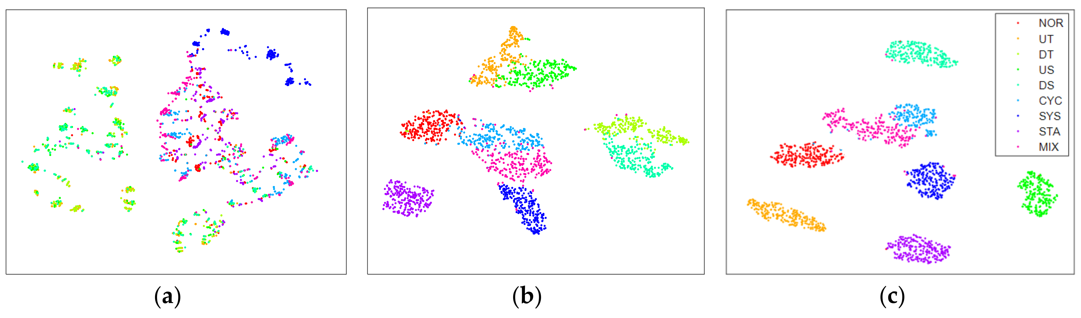
In order to further verify the feature learning ability of multilayer Bi-LSTM to the CCPs, the features extracted from the raw data are visually compared with expert features and the features extracted by 1D-CNN, and the results are shown in Figure 11. In this paper, the t-distributed stochastic neighbor embedding (t-SNE) [52] algorithm is used to reduce the dimensions of feature sets, so that they can be drawn in two-dimensional space for data visualization.
As we know, in the field of pattern recognition, as far as pattern classification is concerned, feature sets should present clustering distribution in feature space. The smaller the distance within the same class, the larger the distance between different classes, indicating that the higher the quality of this feature set, the more conducive to the classification of the classifier. As shown in Figure 11a, the expert feature set has the trend of clustering distribution in the feature space, but the serious cross between each pattern indicates that the quality of existing expert features is not good. This is the root cause of the confusion in Figure 10a. In Figure 11b, the features extracted by 1D-CNN show clustering distribution in the feature space, and the clustering phenomenon increases significantly, but the distance between different patterns is relatively close, and the classifier has the risk of misclassification. In contrast, the features extracted by multilayer Bi-LSTM are more closely distributed in the same pattern, and are better separated from other patterns in the feature space. This shows that it has learned more excellent features from the raw data. In addition, since the features are automatically extracted by the network, the accuracy of pattern recognition is improved, and the workload of quality control personnel is greatly reduced.
4.8. Application in Real Production Data
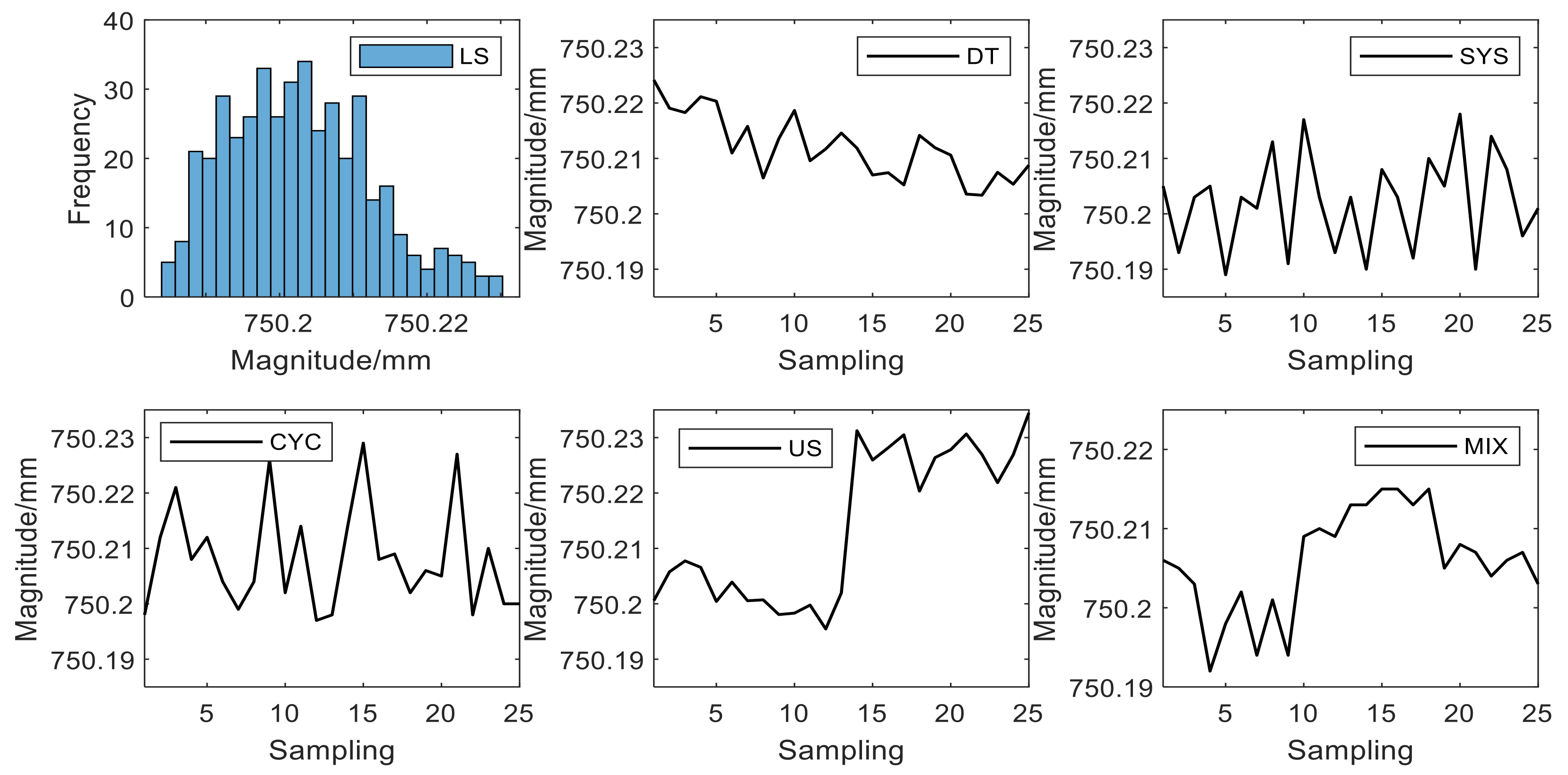
In order to verify the engineering value of the proposed method, it is applied to the quality control of real production. The diameter of the controlled object is the key to judge whether its quality is good or not, and its standard size is mm. The width of the detection window is still 25. The multilayer Bi-LSTM is used to monitor the data of its production process, and some recognition results are listed in Figure 12.
As shown in Figure 12, the proposed method can identify a variety of abnormal patterns from the quality data of the production environment. At the same time, the product quality distribution in this stage is skewed, which is also effectively recognized by the multilayer Bi-LSTM. It can be found that the key dimensions of this batch of products are generally smaller. According to the results of communication with factory engineers, the reason for this histogram pattern is likely to be the result of conscious processing by workers. It is worth noting that the multilayer Bi-LSTM trained with the above simulation data set is used in the quality control of real production data. So before the real data is input into the network, linear transformation is carried out to scale the data to the same range of simulation data. This transformation is very simple and will not affect the speed and automation of recognition. At the same time, it shows that the network trained by the simulation data can identify the real data well, and does not need to train the network repeatedly according to the different product specifications. The proposed method can be easily integrated into the existing industry 4.0 system to provide intelligent SPC data analysis scheme for manufacturing enterprises and improve production efficiency and product quality. In addition, the SYS pattern in Figure 12 was recognized as CYC pattern by 1D-CNN in the previous study [18], which shows that the recognition results of the previous method are not precise enough. In this paper, the CCP is increased to nine, which can achieve more refined CCPR.
5. Conclusions
In order to realize intelligent SPC, this paper proposes a pattern recognition method based on multilayer Bi-LSTM for quality control, which uses feature learning to realize end-to-end HPR and CCPR. After experimental study, the following conclusions can be drawn. First of all, the convergence speed, recognition accuracy and over fitting degree of the network are related to the optimization algorithm, batch size and network layer number, and these parameters should be properly selected. Secondly, after learning, the network can extract the optimal feature set adaptively from the raw data, which has higher quality than the traditional manual expert feature set. Finally, with the raw data as input, the recognition rate of multilayer Bi-LSTM is 99.89% for HPs and 99.26% for CCPs. The recognition accuracy of this model is significantly better than that of traditional methods and other deep learning methods.
To sum up, the proposed multilayer Bi-LSTM method reduces the trouble of manual feature extraction, is competent for HPR and CCPR with high accuracy, and can effectively improve the level of intelligence and automation of SPC. It will likely become an integral part of industry 4.0 technology.
There is still a problem in this study. The length of the control chart and the number of histogram groups input into the network must be fixed, for example, the length of the data in this study is 25. However, in practical application, it may be necessary to adjust the data length to adapt to the production process. The current method must retrain the network, which will cause inconvenience. In the future, we will solve this problem, so that the network can adapt to different data lengths.
Author Contributions
Conceptualization, T.Z. and Z.L.; software, T.Z. and Z.L.; validation, M.W., X.G.; resources, Z.S. and D.C.; writing—original draft preparation, Z.L.; writing—review and editing, T.Z., M.W. and X.G. All authors have read and agreed to the published version of the manuscript.
Funding
This research is supported by China Scholarship Council, grant number 201806545032, and National Natural Science Foundation of China, grant number 51575014, 51875008, and 51975020.
Acknowledgments
The production data used in this study are from Tongyu Heavy Industry Co., Ltd.
Conflicts of Interest
The authors declare no conflict of interest.
References
- Zhou, X.; Jiang, P.; Wang, X. Recognition of control chart patterns using fuzzy SVM with a hybrid kernel function. J. Intell. Manuf. 2018, 29, 51–67. [Google Scholar] [CrossRef]
- Haghtalab, S.; Xanthopoulos, P.; Madani, K. A robust unsupervised consensus control chart pattern recognition framework. Expert Syst. Appl. 2015, 42, 6767–6776. [Google Scholar] [CrossRef]
- Gutierrez, H.D.L.T.; Pham, D.T. Estimation and generation of training patterns for control chart pattern recognition. Comput. Ind. Eng. 2016, 95, 72–82. [Google Scholar] [CrossRef] [Green Version]
- Wang, M.; Zan, T.; Fei, R.Y. Statistical process control with intelligence using fuzzy art neural networks. Front. Mech. Eng. 2010, 5, 149–156. [Google Scholar] [CrossRef]
- Zan, T.; Wang, M.; Fei, R.Y. Pattern recognition for control charts using AR spectrum and fuzzy ARTMAP neural network. Adv. Mater. Res. 2010, 97–101, 3696–3702. [Google Scholar] [CrossRef]
- Yang, W.A.; Zhou, W.; Liao, W.; Guo, Y. Identification and quantification of concurrent control chart patterns using extreme-point symmetric mode decomposition and extreme learning machines. Neurocomputing 2015, 147, 260–270. [Google Scholar] [CrossRef]
- Roberts, S.W. Control chart tests based on geometric moving averages. Technometrics 1959, 1, 239–244. [Google Scholar] [CrossRef]
- Nelson, L.S. Interpreting Shewhart X-bar control charts. J. Qual. Technol. 1985, 17, 114–116. [Google Scholar] [CrossRef]
- Ducan, A.J. Quality Control and Industrial Statistics, 5th ed.; Richard D. Irwin: Homewood, IL, USA, 1986. [Google Scholar]
- Nelson, L.S. The Shewhart control chart: Test for special causes. J. Qual. Technol. 1984, 16, 237–239. [Google Scholar] [CrossRef]
- Ranaee, V.; Ebrahimzadeh, A. Control chart pattern recognition using a novel hybrid intelligent method. Appl. Soft Comput. 2011, 11, 2676–2686. [Google Scholar] [CrossRef]
- Cheng, C.S. A neural network approach for the analysis of control chart patterns. Int. J. Prod. Res. 1997, 35, 667–697. [Google Scholar] [CrossRef]
- Al-Ghanim, A.M.; Ludeman, L.C. Automated unnatural pattern recognition on control charts using correlation analysis techniques. Comput. Ind. Eng. 1997, 32, 679–690. [Google Scholar] [CrossRef]
- Swift, J.A.; Mize, J.H. Out-of-control pattern recognition and analysis for quality control charts using LISP-based systems. Comput. Ind. Eng. 1995, 28, 81–91. [Google Scholar] [CrossRef]
- Cheng, C.; Hubele, N.F. Design of a knowledge based expert system for statistical process control. Comput. Ind. Eng. 1992, 22, 501–517. [Google Scholar] [CrossRef]
- He, S.; He, Z.; Wang, G.A. Online monitoring and fault identification of mean shifts in bivariate processes using decision tree learning techniques. J. Intell. Manuf. 2013, 24, 25–34. [Google Scholar] [CrossRef]
- Kuo, T.; Mital, A. Quality control expert systems: A review of pertinent literature. J. Intell. Manuf. 1993, 4, 245–257. [Google Scholar] [CrossRef]
- Zan, T.; Liu, Z.; Wang, H.; Wang, M.; Gao, X. Control chart pattern recognition using the convolutional neural network. J. Intell. Manuf. 2019. [Google Scholar] [CrossRef]
- Pham, D.T.; Wani, M.A. Feature-based control chart pattern recognition. Int. J. Prod. Res. 1997, 35, 1875–1890. [Google Scholar] [CrossRef]
- Guh, R.S.; Tannock, J. A neural network approach to characterize pattern parameters in process control charts. J. Intell. Manuf. 1999, 10, 449–462. [Google Scholar] [CrossRef]
- Al-Assaf, Y. Recognition of control chart patterns using multiresolution wavelets analysis and neural networks. Comput. Ind. Eng. 2004, 47, 17–29. [Google Scholar] [CrossRef]
- Ranaee, V.; Ebrahimzadeh, A. Control chart pattern recognition using neural networks and efficient features: A comparative study. Pattern Anal. Appl. 2013, 16, 321–332. [Google Scholar] [CrossRef]
- Addeh, A.; Khormali, A.; Golilarz, N.A. Control chart pattern recognition using RBF neural network with new training algorithm and practical features. Isa Trans 2018, 79, 202–216. [Google Scholar] [CrossRef] [PubMed]
- Cheng, Z.; Ma, Y.Z. A Research about Pattern Recognition of Control Chart Using Probability Neural Network. In Proceedings of the Isecs International Colloquium on Computing, Communication, Control, & Management, Guangzhou, China, 3–4 August 2008; IEEE: Piscatway, NJ, USA. [Google Scholar]
- Awadalla, M.H.A.; Sadek, M.A. Spiking neural network-based control chart pattern recognition. Alex. Eng. J. 2012, 51, 27–35. [Google Scholar] [CrossRef] [Green Version]
- Gauri, S.K. Control chart pattern recognition using feature-based learning vector quantization. Int. J. Adv. Manuf. Technol. 2010, 48, 1061–1073. [Google Scholar] [CrossRef]
- Guh, R.S. Real-time recognition of control chart patterns in autocorrelated processes using a learning vector quantization network-based approach. Int. J. Prod. Res. 2008, 46, 3959–3991. [Google Scholar] [CrossRef]
- Yang, W.A.; Zhou, W. Autoregressive coefficient-invariant control chart pattern recognition in autocorrelated manufacturing processes using neural network ensemble. J. Intell. Manuf. 2015, 26, 1161–1180. [Google Scholar] [CrossRef]
- Hachicha, W.; Ghorbel, A. A survey of control-chart pattern-recognition literature (1991–2010) based on a new conceptual classification scheme. Comput. Ind. Eng. 2012, 63, 204–222. [Google Scholar] [CrossRef]
- Xanthopoulos, P.; Razzaghi, T. A weighted support vector machine method for control chart pattern recognition. Comput. Ind. Eng. 2014, 70, 134–149. [Google Scholar] [CrossRef]
- Hu, S.; Zhao, L. A Support Vector Machine Based Multi-kernel Method for Change Point Estimation on Control Chart. In Proceedings of the 2015 IEEE International Conference on Systems, Man, and Cybernetics (SMC), Kowloon, China, 9–12 October 2015. [Google Scholar]
- Pham, D.T.; Oztemel, E. Control chart pattern recognition using learning vector quantization networks. Int. J. Prod. Res. 1994, 32, 721–729. [Google Scholar] [CrossRef]
- Hassan, A.; Baksh, M.; Shaharoun, A.M.; Jamaluddin, H. Improved SPC chart pattern recognition using statistical features. Int. J. Prod. Res. 2003, 41, 1587–1603. [Google Scholar] [CrossRef]
- Pelegrina, G.D.; Duarte, L.T.; Jutten, C. Blind source separation and feature extraction in concurrent control charts pattern recognition: Novel analyses and a comparison of different methods. Comput. Ind. Eng. 2016, 92, 105–114. [Google Scholar] [CrossRef] [Green Version]
- Gauri, S.K.; Chakraborty, S. Recognition of control chart patterns using improved selection of features. Comput. Ind. Eng. 2009, 56, 1577–1588. [Google Scholar] [CrossRef]
- Zhao, C.; Wang, C.; Hua, L.; Liu, X.; Zhang, Y.; Hu, H. Recognition of control chart pattern using improved supervised locally linear embedding and support vector machine. Procedia Eng. 2017, 174, 281–288. [Google Scholar] [CrossRef]
- Janssens, O.; Slavkovikj, V.; Vervisch, B.; Stockman, K.; Loccufier, M.; Verstockt, S.; Van De Walle, R.; Van Hoecke, S. Convolutional Neural Network Based Fault Detection for Rotating Machinery. J. Sound Vib. 2016, 377, 331–345. [Google Scholar] [CrossRef]
- Chen, Z.; Li, W. Multisensor feature fusion for bearing fault diagnosis using sparse autoencoder and deep belief network. IEEE Trans. Instrum. Meas. 2017, 66, 1693–1702. [Google Scholar] [CrossRef]
- Gao, Z.; Ma, C.; Song, D.; Liu, Y. Deep quantum inspired neural network with application to aircraft fuel system fault diagnosis. Neurocomputing 2017, 238, 13–23. [Google Scholar] [CrossRef]
- Fatemeh, A.; Antoine, T.; Marc, T. Tool condition monitoring using spectral subtraction and convolutional neural networks in milling process. Int. J. Adv. Manuf. Technol. 2018, 98, 3217–3227. [Google Scholar]
- Zan, T.; Wang, H.; Wang, M.; Liu, Z.; Gao, X. Application of Multi-Dimension Input Convolutional Neural Network in Fault Diagnosis of Rolling Bearings. Appl. Sci. 2019, 9, 2690. [Google Scholar] [CrossRef] [Green Version]
- Liu, E.; Chen, K.; Xiang, Z.; Zhang, J. Conductive particle detection via deep learning for ACF bonding in TFT-LCD manufacturing. J. Intell. Manuf. 2019. [Google Scholar] [CrossRef]
- Zhao, R.; Yan, R.; Wang, J.; Mao, K. Learning to monitor machine health with convolutional bi-directional lstm networks. Sensors 2017, 17, 273. [Google Scholar] [CrossRef]
- Zhao, R.; Wang, D.; Yan, R.; Mao, K.; Wang, J. Machine health monitoring using local feature-based gated recurrent unit networks. IEEE Trans. Ind. Electron. 2017, 65, 1539–1548. [Google Scholar] [CrossRef]
- Rui, Z.; Ruqiang, Y.; Zhenghua, C.; Kezhi, M.; Peng, W.; Gao, R.X. Deep learning and its applications to machine health monitoring. Mech. Syst. Signal. Process. 2019, 115, 213–237. [Google Scholar]
- Miao, Z.; Yang, M. Control Chart Pattern Recognition Based on Convolution Neural Network. In Smart Innovations in Communication and Computational Sciences. Advances in Intelligent Systems and Computing; Panigrahi, B., Trivedi, M., Mishra, K., Tiwari, S., Singh, P., Eds.; Springer: Singapore, 2019; Volume 670. [Google Scholar]
- Wu, C.; Zhu, B.; Wan, Y.; Zhao, S. Quality Control Chart Pattern Recognition Based on Bidirectional LSTM. Comput. Eng. Softw. 2019, 40, 89–95. (In Chinese) [Google Scholar]
- Simonoff, J.S.; Udina, F. Measuring the stability of histogram appearance when the anchor position is changed. Comput. Stat. Data. Anal. 1997, 23, 335–353. [Google Scholar] [CrossRef] [Green Version]
- Bag, M.; Gauri, S.K.; Chakraborty, S. An expert system for control chart pattern recognition. Int. J. Adv. Manuf. Technol. 2012, 62, 291–301. [Google Scholar] [CrossRef]
- Kingma, D.; Ba, J. Adam: A method for stochastic optimization. arXiv 2014, arXiv:1412.6980. [Google Scholar]
- Zhang, J.; Wang, P.; Yan, R.; Gao, R.X. Deep Learning for Improved System Remaining Life Prediction. Procedia CIRP 2018, 72, 1033–1038. [Google Scholar] [CrossRef]
- Van der Maaten, L.; Hinton, G. Visualizing data using t-SNE. J. Mach. Learn. Res. 2008, 9, 2579–2605. [Google Scholar]
Figure 1.
Quality data and its histogram.

Figure 2.
Seven typical histogram patterns.

Figure 3.
Nine typical CCPs.

Figure 4.
Typical LSTM cell structure.

Figure 5.
The structure of the multilayer Bi-LSTM.

Figure 6.
The training loss under different SGD algorithms.

Figure 7.
The training time and loss under different batch sizes.

Figure 8.
The testing accuracy and training loss under different number of layers.

Figure 9.
The HPR confusion matrix for (a) the MLP and frequency, (b) the DBN and frequency, (c) the 1D-CNN and frequency, and (d) the multilayer Bi-LSTM and frequency.
Figure 9.
The HPR confusion matrix for (a) the MLP and frequency, (b) the DBN and frequency, (c) the 1D-CNN and frequency, and (d) the multilayer Bi-LSTM and frequency.

Figure 10.
The CCPR confusion matrix for (a) the MLP and feature set, (b) the DBN and quality data, (c) the 1D-CNN and quality data, and (d) the multilayer Bi-LSTM and quality data.
Figure 10.
The CCPR confusion matrix for (a) the MLP and feature set, (b) the DBN and quality data, (c) the 1D-CNN and quality data, and (d) the multilayer Bi-LSTM and quality data.

Figure 11.
The feature visualization results for (a) the expert features, (b) the features extracted by 1-CNN, and (c) the features extracted by multilayer Bi-LSTM.
Figure 11.
The feature visualization results for (a) the expert features, (b) the features extracted by 1-CNN, and (c) the features extracted by multilayer Bi-LSTM.

Figure 12.
Abnormal HPs and CCPs found by the multilayer Bi-LSTM from production data.


Table 1.
The simulation parameters of seven typical HPs.
| Patterns | Parameters | Parameter Value/Range |
|---|---|---|
| NOR | Mean μ, standard deviation σ | |
| BIM | Proportion a, offset distance b1 and b2 | |
| LI | Proportion a, offset distance b | |
| RI | Proportion a, offset distance b | |
| LS | The number of normal distributions m | |
| RS | The number of normal distributions m | |
| FT | Proportion a |
Table 2.
The structural parameters and training parameters of multilayer Bi-LSTM.
| Initial Learning Rate | Optimization Algorithm | Batch Size | Number of Layers |
|---|---|---|---|
| 0.05 | Adam | 200 | 3 |
Table 3.
Comparison of different HPR methods.
| MLP & Frequency | DBN & Frequency | 1D-CNN & Frequency | Multilayer Bi-LSTM & Frequency | ||||
|---|---|---|---|---|---|---|---|
| CRR (%) | Time (s/epoch) | CRR (%) | Time (s/epoch) | CRR (%) | Time (s/epoch) | CRR (%) | Time (s/epoch) |
| 96.11 | 4.16 | 98.06 | 0.74 | 99.37 | 1.37 | 99.89 | 4.67 |
Table 4.
The simulation parameters of nine typical CCPs.
| Pattern | Parameters | Mathematical Representation | Parameter Value/Range |
|---|---|---|---|
| NOR | Mean μ, standard deviation σ | ||
| UT | Gradient d | ||
| DT | Gradient d | ||
| US | Shift magnitude s | ||
| DS | Shift magnitude s | ||
| CYC | Amplitude a, Period ω | ||
| SYS | Magnitude g | ||
| STA | Standard deviation σ′ | ||
| MIX | Magnitude m |
Table 5.
Comparison of different CCPR methods.
| MLP & Feature Set | DBN & Quality Data | 1D-CNN & Quality Data | Multilayer Bi-LSTM & Quality Data | ||||
|---|---|---|---|---|---|---|---|
| CRR (%) | Time (s/epoch) | CRR (%) | Time (s/epoch) | CRR (%) | Time (s/epoch) | CRR (%) | Time (s/epoch) |
| 96.40 | 2.03 | 94.04 | 0.91 | 98.44 | 1.83 | 99.26 | 6.32 |
© 2019 by the authors. Licensee MDPI, Basel, Switzerland. This article is an open access article distributed under the terms and conditions of the Creative Commons Attribution (CC BY) license (http://creativecommons.org/licenses/by/4.0/).
Share and Cite
MDPI and ACS Style
Zan, T.; Liu, Z.; Su, Z.; Wang, M.; Gao, X.; Chen, D. Statistical Process Control with Intelligence Based on the Deep Learning Model. Appl. Sci. 2020, 10, 308. https://doi.org/10.3390/app10010308
AMA Style
Zan T, Liu Z, Su Z, Wang M, Gao X, Chen D. Statistical Process Control with Intelligence Based on the Deep Learning Model. Applied Sciences. 2020; 10(1):308. https://doi.org/10.3390/app10010308
Chicago/Turabian StyleZan, Tao, Zhihao Liu, Zifeng Su, Min Wang, Xiangsheng Gao, and Deyin Chen. 2020. "Statistical Process Control with Intelligence Based on the Deep Learning Model" Applied Sciences 10, no. 1: 308. https://doi.org/10.3390/app10010308
Note that from the first issue of 2016, this journal uses article numbers instead of page numbers. See further details here.