Seepage Analysis in Short Embankments Using Developing a Metaheuristic Method Based on Governing Equations

Abstract

Seepage is one of the most challenging issues in some procedures such as design, construction, and operation of embankment or earth fill dams. The purpose of this research is to develop a new solution based on governing equations to solve the seepage problem in an effective way. Therefore, by implementing the equations in the programming environment, more than 24,000 models were designed to be applicable to different conditions. Input data included different parameters such as slopes in upstream and downstream, embankment width, soil permeability coefficient, height, and freeboard. With the use of this big data, a new process was developed to provide simple mathematical models for the seepage rate analysis. The study first used intelligent models to simulate the seepage behavior. Finally, the accuracy of the models was optimized using a new metaheuristic algorithm. This led to the ultimate flexibility of the final model presented as a new solution capable of evaluating different conditions. Finally, using the best model, new mathematical relationships were developed based on this methodology. This new solution can be used as a proper alternative to the governing equations of seepage rate estimation. Another advantage of the proposed model is its high flexibility that can be well applied to engineering design in this field, which was not possible using the initial equations.

1. Introduction

In geotechnical engineering, free surface seepage is one of the main concerns. This seepage can be restricted by flow boundaries with respect to different methods such as Finite Difference Method (FDM) [1] and Finite Element Method (FEM) [2,3,4]. These techniques are based on adaptive meshing and other methods with fixed mesh approaches [5,6,7,8,9,10,11,12,13]. After considering all approaches proposed in the literature to solve the free surface seepage problems, one of the operative approaches, i.e., extended pressure (EP), was selected to be used in this study. This technique is of a high effectiveness since it reduces inequalities of variability into the simpler equalities based on Darcy’s law [14]. This technique is also applied to many types of free surface seepage and numerical purposes [15,16]. In general, the numerical techniques are not used in the engineering field, specifically in the soil mechanics area, mainly because they require rather problematical sources and performances. It means that the experimental tests in the field provide more natural databases compared to the numerical analysis. The basic spreadsheet resolutions for limited seepage problems are presented in some studies when the soil profile includes multiple layers and anisotropic permeability [17]. However, these methods are based on the restricted seepage when the flow boundary condition is recognized. In fact, they do not relate to the unconfined seepage issues such as free surface flows inside the earth dams. In addition to the inner erosion, which is one of the main causes of embankment dam fails, seepage is also a significant factor that needs to be monitored at embankments. In the case of monitoring systems, there are not many cases, but they are sufficient to detect small variations of seepage flow.

For embankment monitoring, two factors need to be checked: temperature and resistivity. Both can help to find specific effects caused by time-dependent processes such as internal erosion, where the comparative accuracy is more critical than absolute accuracy [18]. In terms of dam operation with respect to the instrumentation, dam monitoring is an extremely essential objective. In this area, many monitoring factors are important, including seepage, pore water pressure, deformations, seismic motion acceleration, and temperature amplitudes. Seepage is the most critical issue that may take place during processes related to a dam, e.g., design, construction, and operation. In this context, many earth fill dams have experienced failure of the core section due to the seepage phenomenon. Numerous researchers have attempted to model seepage through earth fill dams using different approaches (e.g., [19,20]). In the case of dam performance based on nonlinear behavior, there are many models that have been developed and introduced in the literature using different methods. These models are generally categorized into three main groups: physics-based, black box, and conceptual models [21].

The FEM model of seepage in embankment soil with piping zone was investigated by Jianhua [22]. It was based on continuum mechanics as a well-known technique to simulate the seepage. He found that the piping zone length and permeability ratio are the most effective factors on the seepage flow. Moreover, PS and Balan [23] studied numerical analysis of seepage in embankment dams. They applied different software such as MODFLOW, SEEP/W, ANSYS, PLAXIS, PDEase2D, and SVFLUX to the analysis of embankment dams in real cases, and also discussed advantages and limitations of the software. In other research, Cho [24] investigated the probabilistic analysis of seepage considering the spatial variability of permeability for an embankment. The traditional seepage analysis method was applied to a layered soil profile to develop a probabilistic approach to interpretation of the uncertainties and spatial variation of the hydraulic conductivity. That study concluded that the developed probabilistic framework can be applied to the hydraulic conductivity of seepage analysis. Le et al. [25] conducted the stochastic analysis of unsaturated seepage in embankment. They used the advantages of both FEM and Monte Carlo simulation techniques to solve the seepage-related problem through a flood defense embankment with random heterogeneous material properties. In another similar study, Calamak et al. [26] presented the probabilistic evaluation of the effects of uncertainty on transient seepage.

Considering the actual physical characteristics of the phenomenon, physics-based and conceptual models are reliable tools, although they have some practical restrictions. Remember that the black box models can be more appreciated when perfect estimates are more significant than physical considerations. Auto Regressive Integrated Moving Average (ARIMA) is a standard black box model that can be used to make an aqua-related time series [27]. These models are linear, hence losing their effectiveness in modeling hydraulic processes that are implanted with high levels of complexity, vitality, and nonlinearity in both spatial and temporal scales. Recently, artificial intelligence (AI) methods have been commonly applied to hydraulic procedures as well as other applications in civil engineering [28,29,30,31,32,33,34,35,36,37,38,39,40,41,42,43,44,45,46,47,48,49,50,51,52,53,54,55,56,57,58,59,60,61,62,63]. AI models such as Feed Forward Neural Network (FFNN), Support Vector Regression (SVR), and Adaptive Neural Fuzzy Inference System (ANFIS) are reasonably new black box approaches which are applicable to different features of hydraulic engineering [64,65,66,67]). To construct a model of dam seepage, Tayfur [68] implemented artificial neural networks (ANNs). They used this method in Poland to predict the piezometric heads on an earth fill dam. Their input data was related to the upstream head and downstream water surface levels to predict the obtained results of FEM. In the case of spatial-temporal modeling of the water level in embankments, an ANN model was proposed by Nourani and Babakhani [69]. They performed ANN modeling to simulate the piezometric water level of an earthen dam. In sole ANN modeling, a single ANN was carried out for each piezometer, whereas in the integrated ANN modeling, a unique ANN was applied to all piezometers at different dam sections. The authors in [70] applied and discussed the Neuro-fuzzy and SVR (based on the Support Vector Machine (SVM)) models as other forms of artificial intelligence approaches. In [71], ANN and fuzzy theories were used in designing an exclusive framework to calculate the water head in piezometers of the Iron Gate 2 dam regarding the tail water levels as input data and the water levels in the piezometers. Lastly, the researchers in [72] employed an SVR model to analyze seepage and dam piping. The use of such black box models (e.g., ARIMA, ANN, ANFIS, and SVR) resulted in reasonable outcomes, although it was also revealed that using different models to solve one definite problem may lead to slightly different consequences. For instance, in a time series prediction, one model may relevantly simulate the maximum assessments, whereas the other may denote well the minimum values. Therefore, as a post-processing method, by linking different models through a collective modeling framework, different aspects of the underlying arrangements may be captured more perfectly. The theory of such a model combination has been already argued and applied to various engineering contexts [73,74,75].

Furthermore, a number of significant studies have been carried out with objectives similar to those of the present paper. ANN-based techniques have been found capable of solving engineering problems; however, they suffer from certain limitations, including low learning speed and incapability of escaping from local minima [76,77]. To remove these disadvantages, ANN can be integrated with optimization algorithms, such as artificial bee colony (ABC), imperialist competitive algorithm (ICA), invasive weed optimization (IWO), and particle swarm optimization (PSO). In this way, bias and weight in ANNs can adjusted, which results in higher efficiency and accuracy level when performing prediction tasks. In recent years, such hybrid systems have been applied to a number of geotechnical problems [78,79,80]. Based on the above discussion, the present paper attempts to accomplish the following objectives:

(1)

Investigating different conditions of the seepage rate in the environment;

(2)

Implementing the equations governing the seepage rate and different generating models;

(3)

Developing neural models;

(4)

Presenting new approaches to evaluating the seepage rate as alternative solutions to the equations previously presented in the literature.

2. Research Methodology

2.1. Theory and Data Collection

There is a need to effectively control the seepage that may occur in earthen embankments in a way to ensure their safety and minimize water loss. With collection of water behind an earthen embankment, a seepage line or saturation line (also called Pheratic line) may appear. This is the line below which positive hydrostatic pressures exist. Right upon the line, pressure is of the atmospheric type, which means that the hydrostatic pressure equals zero, whereas above the seepage line in the capillary fringe, the pressure is negative. Remember that some flow takes place in the capillary fringe, which is normally overlooked in embankment seepage analyses. The location of the seepage line of an embankment needs to be well predicted for three purposes: (1) ensuring that the seepage line is not going to cut the dam downstream face and bring about the toe softening or sloughing; (2) finding the line that separates the wet and dry soil, which is necessary when computing the stability level; and (3) obtaining the top boundary line to draw the flow net, which is needed for calculating the seepage.

The literature consists of a number of studies that suggest determining the discharge and the free surface through homogenous embankment. Such classifications typically utilize the Dupuit’s assumptions. A number of these processes are discussed in the present study.

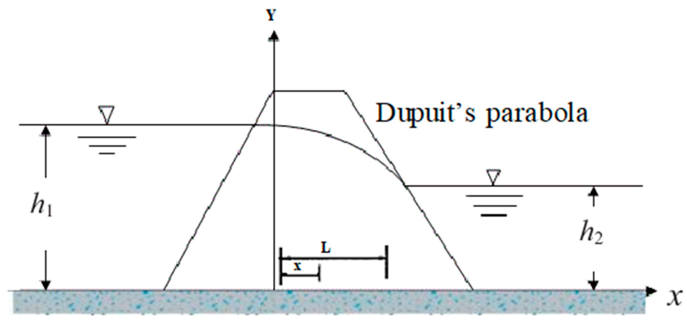
2.1.1. Dupuit’s Method

The discharge per unit width (q) through any vertical section of the dam (Figure 1) is given by

$$\mathrm{q}=-\mathrm{k}\mathrm{y}\frac{dy}{dx}$$

(1)

Integrating and substituting the boundary conditions x = 0, y = h₁ and x = L, y = h₂

$$\mathrm{q}{{\displaystyle \int }}_0^{L}dx=-k{{\displaystyle \int }}_{h1}^{h2}ydy$$

(2)

or

$$\mathrm{q}(\mathrm{L}-0)=-\mathrm{k}[\frac{h_{2-}^2{h}_1^2}{2}]$$

(3)

Therefore,

$$\mathrm{q}=-\mathrm{k}[\frac{h_{2-}^2{h}_1^2}{2L}]$$

(4)

A parabolic function is needed in this equation in regard to free surface, which is generally recognized as Dupuit’s parabola [81]. According to the study conducted by Murty [81], no study has been carried out taking into account the emerging or exiting situations of the seepage line or the development of a surface of seepage. With no water level upon the downstream (h₂ = 0), indeed the seepage line intersects the impervious base that is called bedrock. Furthermore, it is worth mentioning that neither the locus of the free surface nor the discharge capacity depends on the slopes.

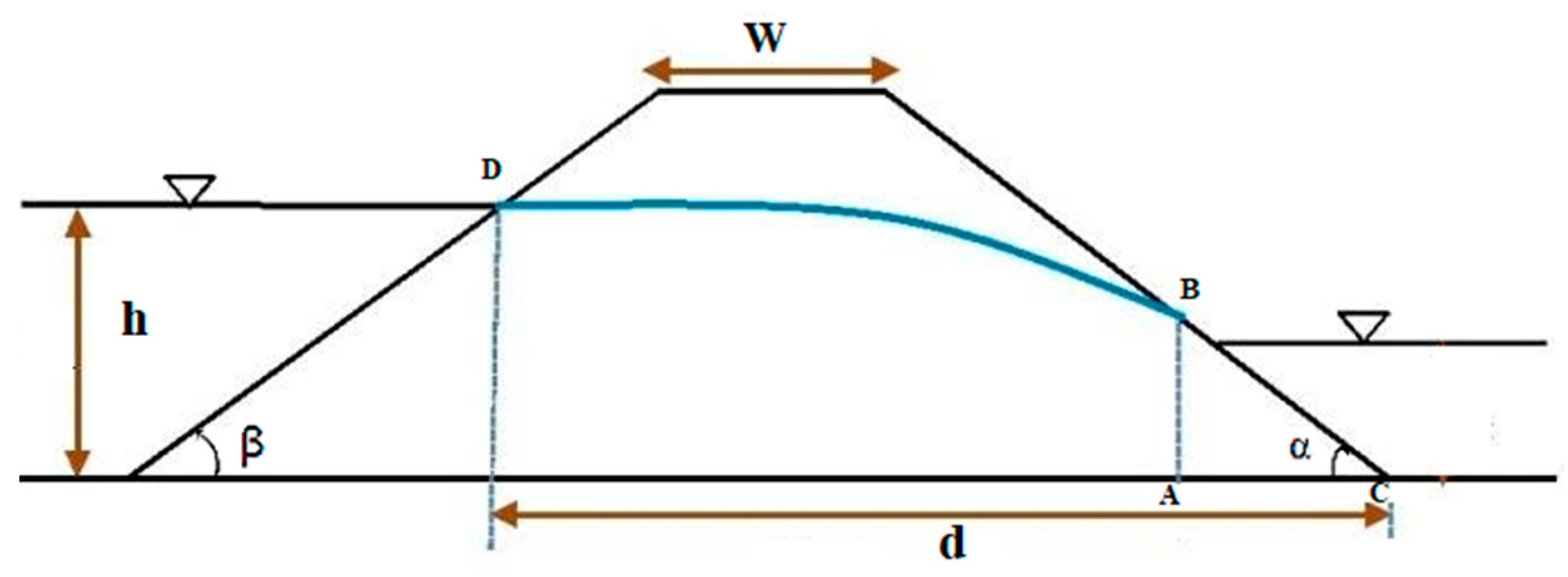
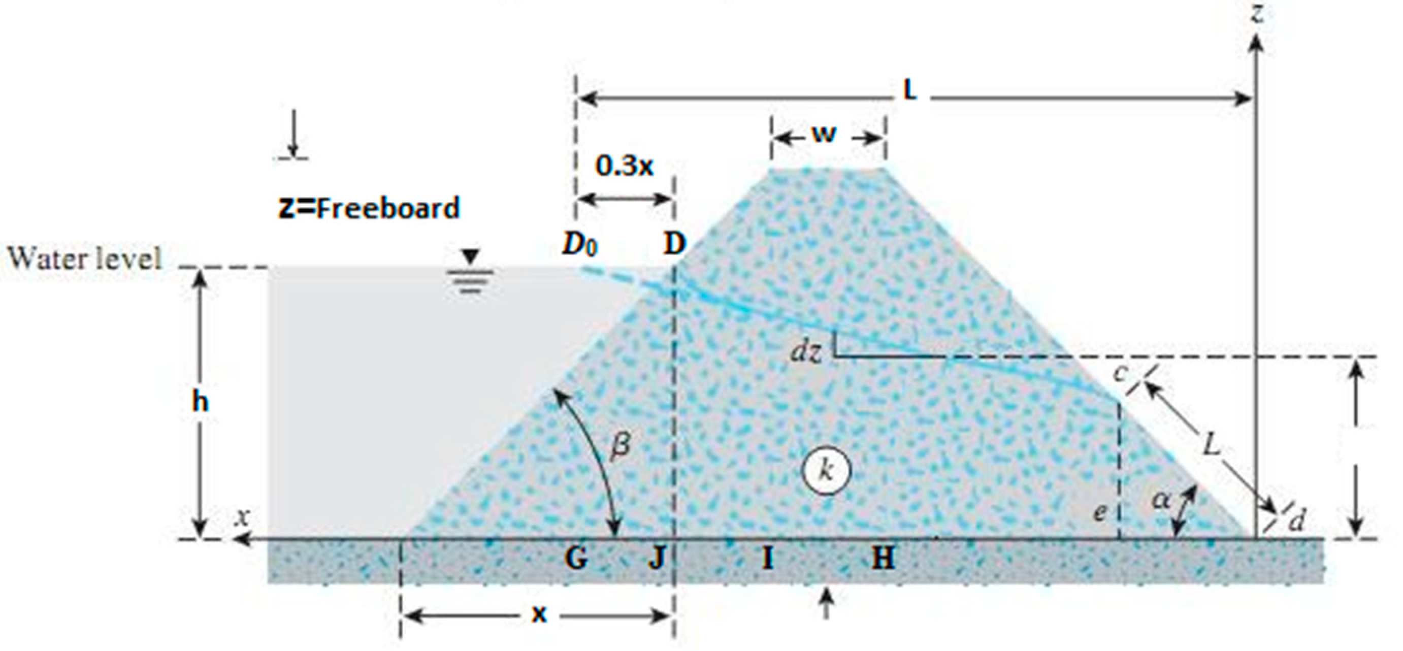
2.1.2. Schafferank and van Iterson Method

The first approximate method for the development of free surface was proposed by Schaffernak and van Iterson [81].

As an earthen embankment on an impervious base (Figure 2) with no tail water, and with applying Equation (1) to triangle CAB, the discharge per unit width (with x taken as + ve to the left) can be achieved:

$$\mathrm{q}=-\mathrm{k}\mathrm{y}\frac{dy}{dx}=\mathrm{k}\mathrm{a}\sin \mathsf{\alpha }.\tan \mathsf{\alpha }$$

(5)

where a denotes the length of seepage surface, and K stands for hydraulic conductivity of the embankment material. Equation (5) can be used to determine the value of ‘a’.

$$\mathrm{q}{{\displaystyle \int }}_{asin\alpha }^{h}ydy={{\displaystyle \int }}_{asin\alpha }^{d}asin\alpha .tan\alpha dx$$

(6)

Or,

$$\frac{1}{2}(h^2-a^{2}si{n}^2\alpha =asin\alpha .tan\alpha \left(d-acos\alpha \right)$$

(7)

Or,

$$(h^2-a^{2}si{n}^2\alpha =2ad\frac{si{n}^2\alpha }{cos\alpha }-2a^{2}si{n}^2\alpha$$

(8)

Or,

$$a^2-\frac{2d}{cos\alpha }a+\frac{h^2}{si{n}^2\alpha }=0$$

(9)

Or,

$$a=\frac{1}{2}[\frac{2d}{cos\alpha }-\sqrt{\left(\frac{4d^2}{co{s}^2\alpha }-\frac{4h^2}{si{n}^2\alpha }\right)}]$$

(10)

Therefore,

$$a=\frac{d}{cos\alpha }[\sqrt{\left(\frac{d^2}{co{s}^2\alpha }-\frac{h^2}{si{n}^2\alpha }\right)}]$$

(11)

Remember that the parabolic free surface in this case is tangent to the downstream slope, which is not the case with the Dupuit’s solution. This plays a critical role for the entrance conditions correction at the upstream slope. As suggested by Casagrande, point D₀ (Figure 3) is better to be taken as the starting point of a seepage line, rather than point D. As can be seen, distance between $D_0$ and D is 0.3 X. In fact, X is OJ. It means that $D_0$D as a distance depends on upstream slope (β). After that, the actual entrance condition can be determined through sketching in the area DF tangent to the parabolic free surface and normal to the upstream slope.

In case of a homogenous embankment that is positioned upon an impervious foundation in which the discharge slopes are flatter than 1:1 (see Figure 3), a possible assumption is that the point where the seepage line and the downstream face are intersected is as expressed below:

$$e=asin\alpha =\frac{h}{3}$$

(12)

where e stands for the distance between the impervious base and the intersection of the seepage line upon the downstream side, and h signifies the height of water upon the upstream side.

The discharge through a unit width of embankment (q) is obtainable through the use of Darcy’s law:

$$\begin{array}{ll}q& =-\mathrm{k}\mathrm{y}\frac{dH}{dL}\times \mathrm{Area}\left(\mathrm{mean}\mathrm{discharge}\mathrm{area}\mathrm{of}\mathrm{vertical}\mathrm{cross}\mathrm{section}\right)\\ & =-\mathrm{k}\left(\frac{e-h}{L}\right)\times \left(\frac{h+e}{2}\times 1\right)\\ & =\mathrm{k}\left(\frac{h-e}{L}\right)\times \left(\frac{h+e}{2}\right)\\ & =\frac{k}{2}\left(\frac{h^2-e^2}{L}\right)\end{array}$$

(13)

where k stands for hydraulic conductivity of the material of the embankment or permeability coefficient, and L denotes the mean length of the seepage line (the distance from the starting point of the seepage line D₀ to the midpoint A of the seepage face BC).

Replacing for e = h/3 in Equation (14) we will obtain:

$$\begin{gathered} q=\frac{k}{2}\left(\frac{h^2-{\left(\frac{h}{3}\right)}^2}{L}\right) \\ \mathrm{Or}, \\ \mathrm{q}=\left(\frac{h4k{h}^2}{9L}\right) \end{gathered}$$

(14)

In Figure 3, L is given by

$$\begin{array}{ll}L& =\mathrm{EG}\\ & =\mathrm{EH}+\mathrm{HI}+\mathrm{IJ}+\mathrm{JG}\\ & =(\mathrm{C}\mathrm{H}-\mathrm{C}\mathrm{E})+\mathrm{H}\mathrm{I}+\mathrm{I}\mathrm{J}+\mathrm{J}\mathrm{G}\\ & =(\mathrm{h}+\mathrm{Z})\cot \mathsf{\alpha }-\frac{e}{2}\cot \mathsf{\alpha }+\mathrm{W}+\mathrm{Z}\cot \mathsf{\alpha }+0.3\mathrm{m}\\ & =(\mathrm{h}+\mathrm{Z})\cot \mathsf{\alpha }-\frac{e}{2}\cot \mathsf{\alpha }+\mathrm{W}+\mathrm{Z}\cot \mathsf{\alpha }+0.3\mathrm{h}\cot \mathsf{\alpha }\\ & =(1.3\mathrm{h}+2\mathrm{Z})\cot \mathsf{\alpha }-\frac{e}{2}\cot \mathsf{\alpha }+\mathrm{W}\\ & =(1.3\mathrm{h}+2\mathrm{Z}-\frac{e}{2})\cot \mathsf{\alpha }+\mathrm{W}\end{array}$$

(15)

where Z denotes the vertical distance from upstream water level to the top of embankment, W signifies the top width of the embankment, and α represents the angle of the downstream and upstream faces.

The seepage formula is applied to a coding program with respect to the visual basic language using Excel 2014. Based on the scope of study, input data are used to extract the output data that is the seepage rate for homogenous embankment. A total of 24,197 models were taken into consideration in this study. In this paper, the soil permeability coefficient (K) is between 1 × 10⁻⁴ to 1 × 10⁻¹⁰ cm/s, height water (HW) is between 15 m and 50 m, freeboard (FB) is between 2 m and 5 m, upstream slopes (β) are between 15° and 30°, downstream slopes (α) are between 15° and 30°, and width crest (WC) is between 8 m and 12 m. After all this, the output data, which are Q (m³/s) with respect to seepage rate, are computed for all models.

Table 1. The statistical details of the dataset in this research.

Parameter	Abbreviation	Unit	Min	Max	Average	Std
Soil permeability coefficient	K	cm/s	1 × 10−10	1 × 10−4	1.59 × 10−5	3.45 × 10−5
Height water	HW	m	10	48	29	10.89
Freeboard	FB	m	2	5	4	1.12
Upstream slopes	β	degree	15	30	23	5.59
downstream slopes	α	degree	15	30	23	5.59
Width crest	WC	m	8	12	10	1.63
Seepage rate	Q	m3/s	7.81 × 10−11	1.48 × 10−3	8.82 × 10−5	2.22 × 10−5

presents the statistical details of the data.

2.2. Prediction Models

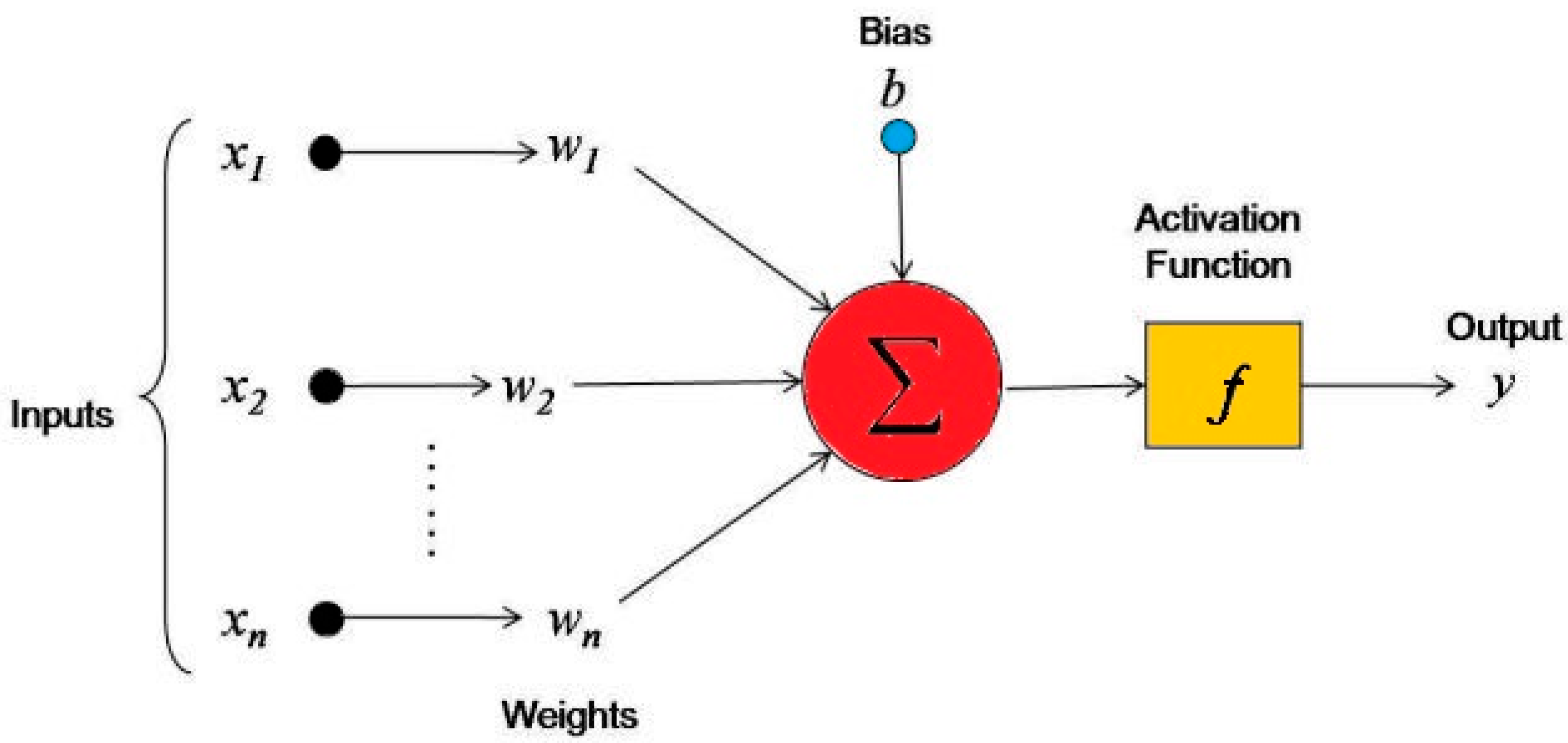
2.2.1. Artificial Neural Network (ANN)

Artificial neural network (ANN), which was introduced by McCulloch and Pittsin [82], is an intelligence mathematical technique of high popularity. This technique is capable of mimicking the complicated nonlinear relationships between input and output parameters on the basis of various environments. It is actually a simulation of the human brain neural mechanisms. ANN is an efficient parallel processing architecture containing at least a single hidden layer as well as input and output variables. It effectively handles fuzzy information where the functional relationships are not clear [80,83,84]. In ANN, through training, preceding samples, and experiences, the models can be created. It can be said that based on various training data, those patterns that are utilized to collect the neurons and outputs are mutative. Neurons construct the foundation of an ANN; they form the network organization. The neurons construct the layer(s) and the contextual layers have connection with each other through interconnection weights. ANN has been presented in lots of patterns among which the feed-forward-back-propagation (BP) is of a high practicality and has been used effectively in a number of studies [85,86,87]. Various inputs exist in each neuron. In the course of a training process, an output is produced by these inputs. Within ANN, neurons are in a full connection with each other, and the output of each unit element will be used as a new input for the following unit element. The layers in this system are composed of multiple neurons; the information is transmitted from the first layer to the next one in the course of training process and then the network response is produced by the last layer. The intermediate layers (also called hidden layers) are located between the input and output layers [88]. Numerous algorithms have been proposed in the literature on the basis of ANN; among them, BP is recognized of the highest popularity when there is a need for the interpretation of the network modification behavior [89]. In general, the error correction learning law is implemented in BP in which the error propagation actually adjusts the connection weights in a way to decrease as much as possible the sum of the mean squared error within the output layer. That is, the learning propagation comprises two phases: forward phase and back phase. In the former, a series of outputs is provided by the layer inputs transmission. In the latter, synaptic weights are obtained. To evaluate the efficiency of the above-mentioned model performance, two statistical indicators are taken into account, namely the coefficient of determination (R²) and the root mean square error (RMSE) [90,91].

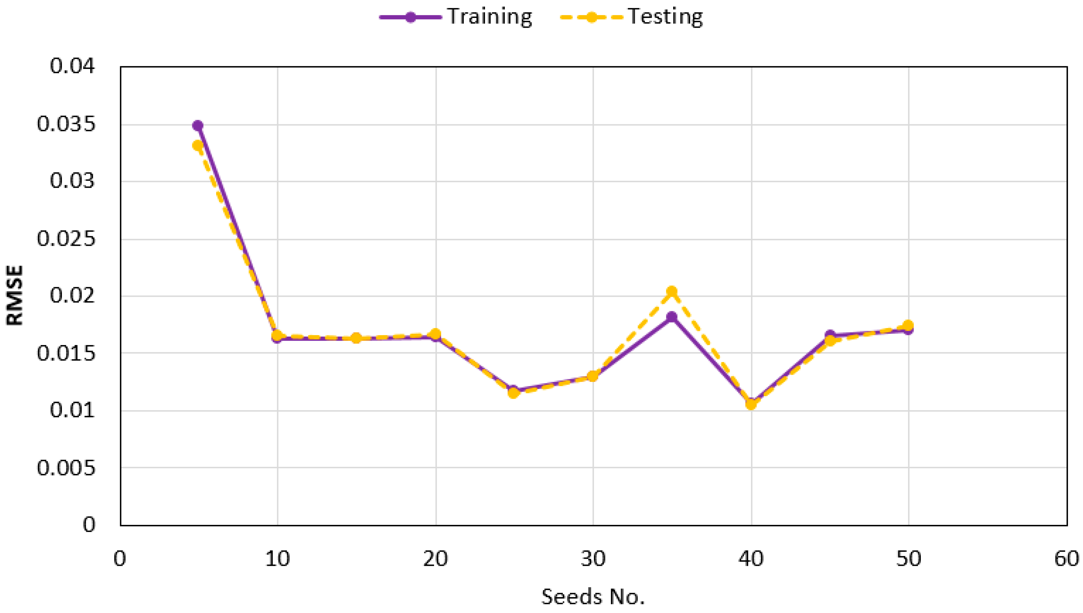
2.2.2. Invasive Weed Optimization (IWO)

The invasive weed optimization (IWO) is an optimization algorithm that works based on population. It is capable of satisfying the high quality performance of a mathematical equation through adapting and randomizing a weed colony. The rapid and wide growth of weeds is a significant threat to agricultural products. They show a great resistance to environmental and climate changes. As a result, a strong optimization algorithm can be designed by simulating the behaviors of this herb. In fact, IWO makes use of the weed community and their high level of resistance, compatibility, and randomness in order to find an effective solution to a given problem.

Researchers have developed IWO on the basis of agriculture phenomena inspired by the invasive weeds. As mentioned earlier, weeds have the capacity of growing unintentionally. However, scientists have noted numerous benefits for the presence of this herb in urban spaces. Only due to some damage that the unintentional growth of weeds may have for human activities and the planet’s life, is it recognized as a “weed” [92]. Though IWO is an algorithm of an acceptable simplicity regarding the concept, structure, and implementation, it is known as a robust optimization algorithm with a high capacity for solving nearly all optimization problems. In the following, the IWO operation is explained step by step:

(1)

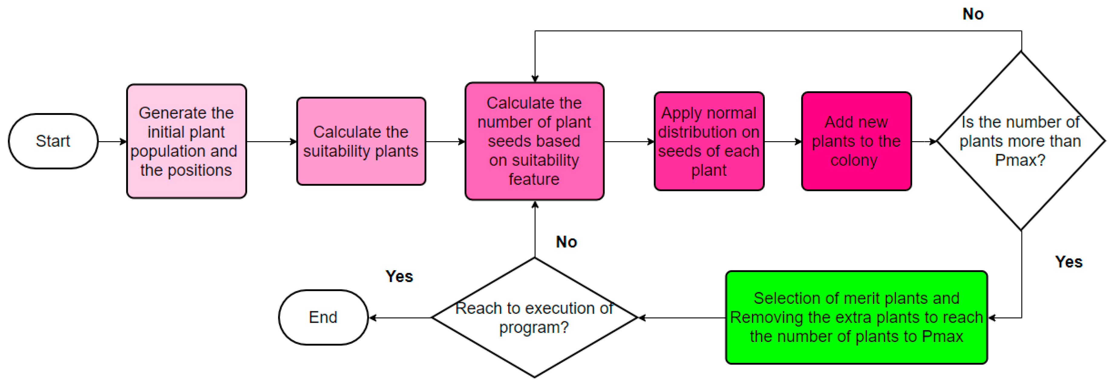
First, at the “population initialization” step, several seeds are randomly distributed within the search space.

(2)

At the “reproduction” step, every plant is poured into a flowering plant; after that, the system can produce seeds that are worth their proportion. Then, the quantity of the seeds is linearly reduced from Smax to Smin with the use of the following equation:

$$n(w_i)=\frac{S_{\max }(\max fit-fit(w_i))+S_{\min }(fit(w_i)-\min fit)}{\max fit-\min fit}$$

(16)

(3)

At the third step, a new position of the seeds within the search space is determined. At this step, the child’s seeds are positioned nearby their parents.

(4)

At the fourth step, which is referred to as the competitive elimination step, the best seeds are created based on their merit. It takes place in the case that a certain number (Pmax) of seeds have been created.

(5)

Finally, at the fifth step, if the termination criterion is not satisfied yet, the whole process is repeated from the second step to the end. It continues until the termination criterion is met, and the algorithm operation will then end. Figure 4 illustrates a general diagram showing the steps involved in an IWO operation.

2.2.3. Hybrid Algorithms

The literature contains numerous study conducted to improve ANN using optimization algorithms like PSO, GA, ICA, and ABC (see [38,93,94,95,96,97,98]). BP does not act strongly in exploring the accurate global minimum; as a result, the ANN model might obtain unwanted results [99]. However, there is a higher probability for ANN to be trapped in local minima. In this regard, optimization algorithms are able to address the above-noted problem effectively through setting the biases and weights of ANN. The present paper develops a new hybrid model: IWO-ANN, for the purpose of predicting seepage rate. In this hybrid model, IWO is responsible for exploring the global minimum; after that, ANN chooses it in a way to obtain the best results.

3. Simulation Models

Hybrid model processes are presented in this section. A new hybrid model that is based on the combination of the base model (ANN) with the algorithm of IWO is discussed. To design the best model to predict the seepage rate, each model is separately evaluated to identify the best performance of each.

3.1. Initial Model

This section explains the way an ANN model was designed and developed in order to predict the seepage rate. To design an effective intelligent system, an important step is the proper use of input data. The literature was reviewed to identify the parameters that can affect the seepage rate.

Table 2. Results of various artificial neural network (ANN) models with activation function Tanh.

Model No.	Structure	The Best R2
		Training	Testing
T1	6-1-1	0.7925	0.8050
T2	6-2-1	0.9126	0.9068
T3	6-3-1	0.8738	0.8633
T4	6-4-1	0.9018	0.9184
T5	6-5-1	0.9378	0.9333
T6	6-6-1	0.9140	0.9050
T7	6-7-1	0.8919	0.8998
T8	6-8-1	0.9071	0.9199
T9	6-9-1	0.9155	0.9143
T10	6-10-1	0.9241	0.9077

presents the input data applied to the proposed model. Every intelligent network consists of two basic parts: training and testing. The former creates a nonlinear relationship between independent and dependent variables, while the latter examines the first part. Therefore, out of the total 24,000 pieces of data accessible here, there is a need to determine a portion applicable to training processes and another to testing processes. As widely suggested in the literature by various researchers, [33,55,56,57,58], 80% of data was allocated to training and the remaining part was allocated to testing.

A variety of algorithms have been introduced in the literature for the purpose of training ANN, among which a key one is the Levenberg–Marquardt (LM) method [100,101,102,103,104]. It can be effectively applied to problems that may arise in the civil engineering and mining contexts [60,61,62]. Three layers exist in this model; the first and third layers are related to the input and output data, respectively. In studies carried out formerly, a hidden layer has been also utilized for solving many linear and nonlinear engineering problems [105,106,107,108]. For that reason, in this study, a hidden layer is also used. Figure 5 presents the ANN structure implemented in this paper.

The principal objective of the ANN model is the exploration of a proper way through which the intelligent systems could perform their defined predictive tasks. Typically, two parameters have impact on performance of the ANN models: the number of neurons and the number of iterations. More specifically, the number of neurons existing in the hidden layer meaningfully contributes to determination of the minimum limits of computational space. This study continues toward the phases that are set on the basis of the initial conditions of the under-consideration problem. If the initial conditions cannot be met, the system then continues working on the basis of a predefined number of iterations. The literature consists of various approaches to determining the optimum number of neurons that can exist in the hidden layer. To this end, different researchers have suggested different formulas [104,109,110]. Nevertheless, in the engineering field, numerous studies have implemented various numbers of data, which shows that the intelligent models demonstrate their best performance in every computational space with a certain number of neurons [105,111]. Moreover, a complete analysis of 10 to 100 iterations was done in order to specify the number of iterations. The value of 80 iterations was selected by sensitivity analysis as the value that requires the best results. Additionally, R² and RMSE were employed as statistical indices in order to evaluate the developed model’s performance quality. In this study, in addition to the number of neurons, activation functions were also investigated as affecting parameters. In the neural models, the famous function was used for this research: Tanh, Exponential, Sine and Logistic.

Finally, 5 groups of different neural network structures were developed for seepage rate. The results of these groups are presented in Table 2,

Table 3. Results of various ANN models with activation function Exponential.

Model No.	Structure	The Best R2
		Training	Testing
E1	6-1-1	0.8460	0.8391
E2	6-2-1	0.9025	0.8954
E3	6-3-1	0.9257	0.9261
E4	6-4-1	0.9059	0.9064
E5	6-5-1	0.8648	0.8660
E6	6-6-1	0.8813	0.8956
E7	6-7-1	0.9103	0.9213
E8	6-8-1	0.9052	0.9149
E9	6-9-1	0.8666	0.8926
E10	6-10-1	0.8860	0.8722

,

Table 4. Results of various ANN models with activation function Sine.

Model No.	Structure	The Best R2
		Training	Testing
S1	6-1-1	0.8571	0.8600
S2	6-2-1	0.8708	0.8924
S3	6-3-1	0.9231	0.8874
S4	6-4-1	0.8962	0.9053
S5	6-5-1	0.8862	0.9113
S6	6-6-1	0.9055	0.8813
S7	6-7-1	0.8834	0.9075
S8	6-8-1	0.9017	0.8825
S9	6-9-1	0.8876	0.9175
S10	6-10-1	0.8668	0.8925

and

Table 5. Results of various ANN models with activation function Logistic.

Model No.	Structure	The Best R2
		Training	Testing
L1	6-1-1	0.8513	0.8643
L2	6-2-1	0.8757	0.8875
L3	6-3-1	0.8521	0.8432
L4	6-4-1	0.8852	0.8946
L5	6-5-1	0.9023	0.8904
L6	6-6-1	0.8938	0.8849
L7	6-7-1	0.8759	0.9009
L8	6-8-1	0.9052	0.8944
L9	6-9-1	0.8707	0.8712
L10	6-10-1	0.8802	0.8934

, respectively. As can be seen, the prediction of seepage rate generally performs well. However, these tables show that each different activation function and structure of the hidden layer neurons have different functions. In designing intelligent networks, the system needs to be carefully evaluated for under-fitting and over-fitting. According to the system trends, the results do not have the first problem (under-fitting), but do have the second problem (over-fitting), which is more common and must be carefully considered. According to the results, models T5, E3, S3, and L8 are the best-designated screens. With regard to the over-fitting problem, it can be seen that structures of S3 and L8 have lower prediction accuracy of the testing section against the high accuracy of the training section. This indicates that the system has not been able to properly accommodate all conditions. This suggests that models are more trained and less flexible with new data. Finally, among all models, Model T5 with accuracy of 0.9378 and 0.9333 for both training and testing sections, respectively, is presented as the best structure for seepage rate prediction. This structure is then combined with an IWO algorithm and a new structure (IWO-ANN) is introduced to increase its performance.

3.2. Hybrid Model Development

This section describes the implementation of the new IWO-ANN model. A review of the literature revealed that no study has been already conducted integrating ANN and IWO, though this new model is implemented in the same way as the parallel models. The above-mentioned IWO algorithm is indeed an innovative optimization algorithm applicable to different problems. This algorithm involves different parameters among which the key ones include the seeds’ initial population and the number of iterations. A number of parameters in this regard exert less effect upon the finally obtained results and they can be achieved through a trial-and-error approach. As a result, such parameters are determined at the beginning of the algorithm operation. For instance, the minimum (Smin) and maximum (Smax) number of seeds were examined in a range between 0 and 30. It was found that the Smin value is zero and the optimal value of Smax is 25. The initial and final values of the standard deviation parameter, which provides a great help to knock off the selection, can be obtained with the use of the variance reduction exponent parameter. The three parameters of the initial and final values of the standard deviation and the variance reduction exponent were set to 5.0, 0.001, and 2, respectively. Finally, the main parameters such as the number of iterations and the number of seeds were determined according to Figure 6, Figure 7, Figure 8 and Figure 9.

Figure 6 shows the iteration changes for different models. As can be seen, the two models with the repetition of 300 and 400 provide the best case for seepage rate prediction. Here, by examining the testing section, it can be seen that the performance of the model is reduced by 400 iterations. This indicates that the model is over-fitting, indicating that the model does not have the capability to handle new data. For this reason, the model with 300 iterations provides greater flexibility due to the close proximity of both training and testing sections. As a result, this model is chosen. The RMSE results of the models are also shown in Figure 7. As can be seen, the RMSE of model with 300 and 400 iterations is less than other models, but since the system with 400 iterations has increased errors against new data (testing dataset), it excludes the selected options. Finally, by examining Figure 9 and Figure 10 and considering the different operating conditions of the models, the model with the repetition of 300 is chosen as the main model. In the following, the study is performed for the number of seepage rate with 300 iterations (Figure 8 and Figure 9). As the number of seeds increases, the R² of system first increases and then slightly decreases. Figure 8 shows the changes of R². As can be seen, the 30-seed model offers the best performance. By examining the testing section of the model, it can be concluded that the model has high ability to deal with new data. Figure 9 shows the model RMSE variations, which generally reduce the error and the best model, with the number of 30 seeds. Finally, the model with the number of 300 iterations and 30 seeds was obtained as the best predictive model for seepage rate. As can be seen, the best IWO-ANN model performs better than the basic neural network models developed in the previous section. This indicates a successful improvement for the new IWO-ANN method. The various applications of the model are discussed below.

4. Results and Discussion

This section discusses the models developed in the previous section. As mentioned earlier, the seepage equations in earth dams and embankments were first implemented and then coded, then the different conditions of these equations were investigated. Finally, a dataset containing 24,000 datasets evaluating different aspects was created. Then, neural and hybrid models were developed to provide a new solution for seepage rate estimation. Different models of the neural network were developed and finally the best model was improved by the IWO algorithm in order to increase its capacities in the simulation. This final model was used to evaluate the seepage rate as a new solution for all data. The results of the two sections of training and testing are presented in Figure 10 and Figure 11. As can be seen, the new solution has been able to offer high potential as an alternative to the equations governing for seepage rates in the defined condition.

By examining the equations and the new hybrid model, it is determined that the soil permeability coefficient (K) parameter is the most effective reason for the seepage rate. Therefore, for conditions where the soil permeability coefficient (K) parameter is constant for the environment, the influence of other parameters is evaluated. It should be noted that in reality, simplification conditions are also used for the same permeability to the environment. However, the new hybrid system will be able to simplify the equations that exist between each parameter and the seepage rate. For the water height, freeboard, upstream slope, downstream slope, and width crest parameters in Figure 12, Figure 13, Figure 14, Figure 15 and Figure 16, the influence of each parameter is presented. As can be seen, due to the high accuracy of the hybrid model, the evaluation of each parameter is also very accurate. This demonstrates the generalization power of these new hybrid systems. The influence of each parameter shows what optimal solutions can be used to design specific conditions for the seepage rate. In addition, this new methodology helps engineers deliver the best design at a lower cost. Finally, the new equations obtained by the hybrid model analyses are presented in

Table 6. The equations between the parameters and seepage rate (x and y indicate the parameters and seepage rate in the equations).

The Parameters	Equation	R2
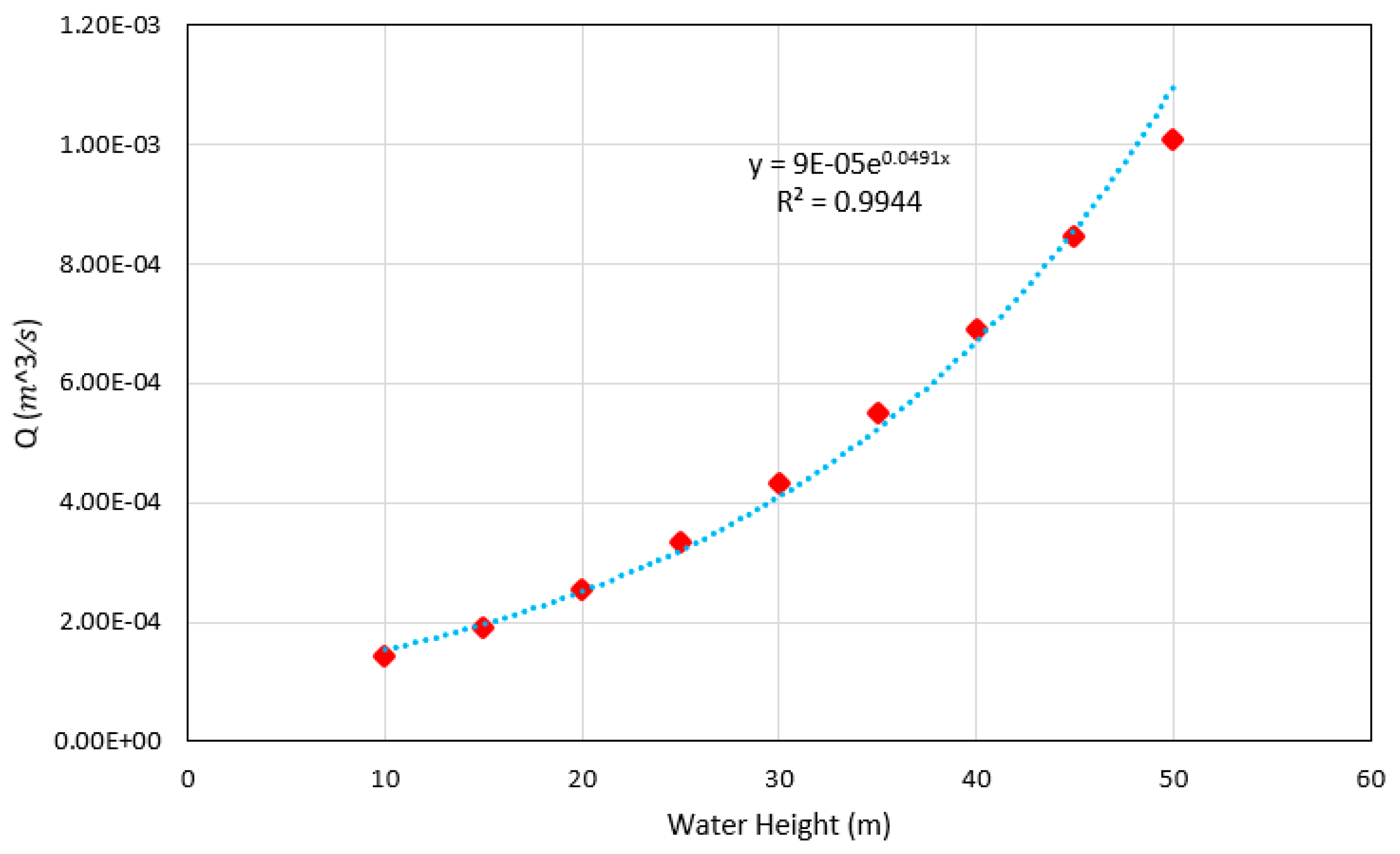
Water height	Y = 9 × 10−5 ${\mathrm{e}}^{0.0491\mathrm{x}}$	0.9944
Freeboard	Y = −8 × 10−6 x + 0.0002	0.9994
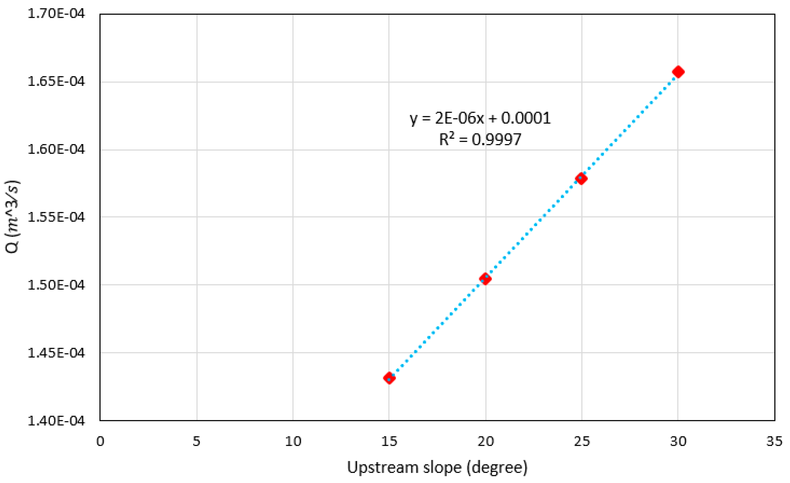
Upstream slope	Y = 2 × 10−6 x + 0.0001	0.9997
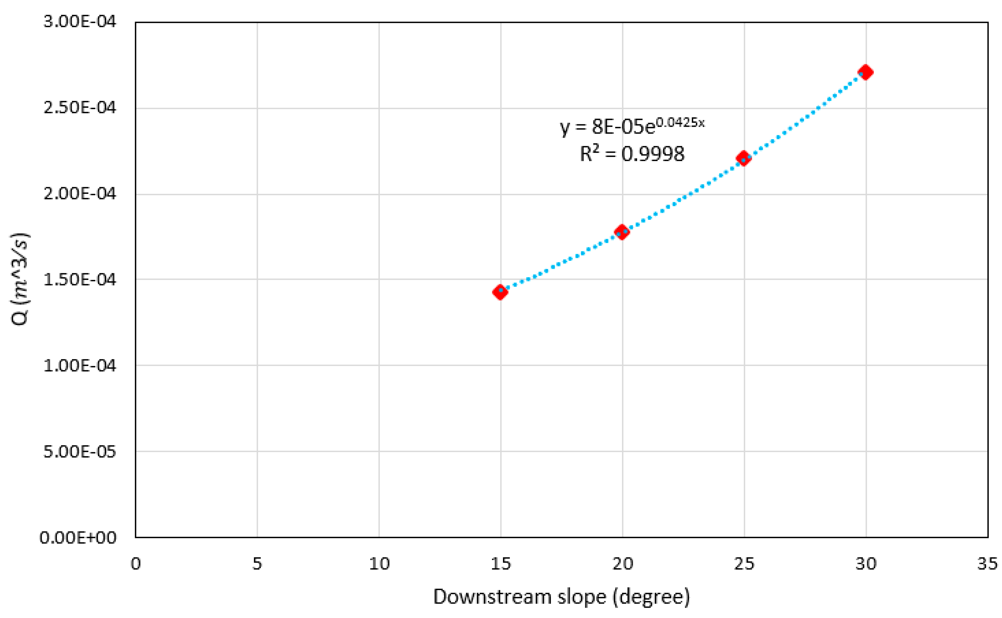
Downstream slope	Y = 8 × 10−6 ${\mathrm{e}}^{0.0425\mathrm{x}}$	0.9998
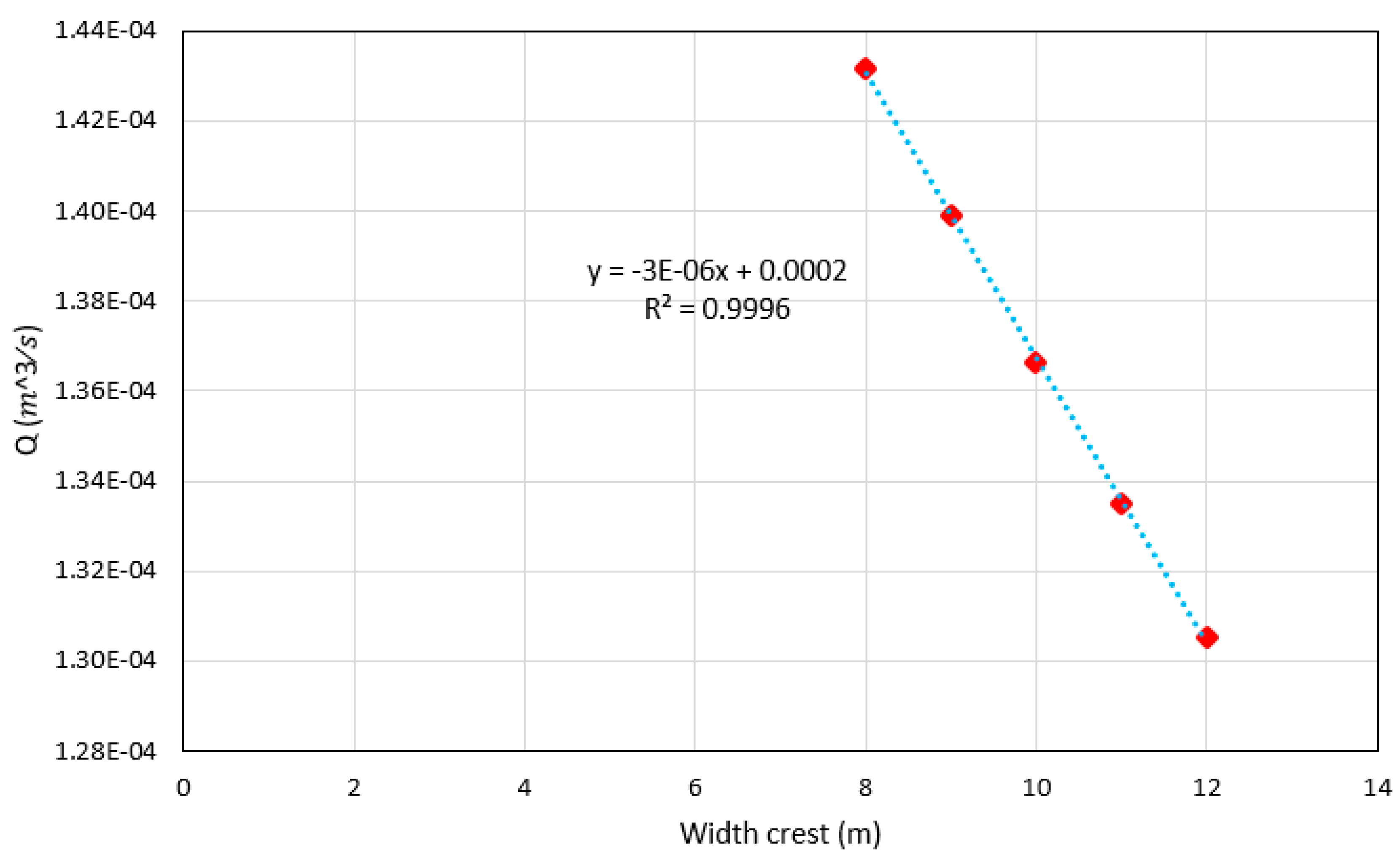
Width crest	Y = −3 × 10−6 x + 0.0002	0.9996

. These new equations presented under the new solution can find many applications due to their simplicity.

5. Conclusions

In this research, we developed new methods for modeling seepage rate in earth dams and embankments. The purpose of this research was to use alternative techniques to mathematical models to gain more capabilities. Therefore, mathematical models for seepage rate within different environments were discussed and then different design conditions were considered. More than 24,000 different models were defined. The dataset contained 6 parameters: soil permeability coefficient (K), water height (WH), freeboard (FB), upstream slopes (β), downstream slopes (α), and width crest (WC). Due to their importance, artificial neural networks (ANN) were implemented. The accuracy of this problem was discussed due to finding alternative mathematical solutions. Therefore, early neural models were designed with different conditions. Finally, the best one was combined with the invasive weed optimization (IWO) algorithm. The combination of the two models created a new model called the IWO-ANN. This model offers a more generalized power to evaluate seepage rate. Finally, using this model, new and simpler relationships for each parameter were presented. These new formulas offer simpler solutions, greater generalization power, and the flexibility to evaluate different seepage rate engineering requirements. This research can be extended to other areas of engineering as a new methodology.

References

- Cryer, C.W. On the approximate solution of free boundary problems using finite differences. J. ACM 1970, 17, 397–411. [Google Scholar] [CrossRef]
- Taylor, R.L.; Brown, C.B. Darcy flow solutions with a free surface. J. Hydraul. Div. 1967, 93, 25–33. [Google Scholar]
- Finn, W.D. Finite-element analysis of seepage through dams. J. Soil Mech. Found. Div. 1967, 93, 41–48. [Google Scholar]
- Neuman, S.P.; Witherspoon, P.A. Finite element method of analyzing steady seepage with a free surface. Water Resour. Res. 1970, 6, 889–897. [Google Scholar] [CrossRef] [Green Version]
- Westbrook, D.R. Analysis of inequality and residual flow procedures and an iterative scheme for free surface seepage. Int. J. Numer. Methods Eng. 1985, 21, 1791–1802. [Google Scholar] [CrossRef]
- Baiocchi, C. Su un problema di frontiera libera connesso a questioni di idraulica. Ann. Mat. Pura Appl. 1972, 92, 107–127. [Google Scholar] [CrossRef]
- Bathe, K.; Khoshgoftaar, M.R. Finite element free surface seepage analysis without mesh iteration. Int. J. Numer. Anal. Methods Geomech. 1979, 3, 13–22. [Google Scholar] [CrossRef] [Green Version]
- Alt, H.W. Numerical solution of steady-state porous flow free boundary problems. Numer. Math. 1980, 36, 73–98. [Google Scholar] [CrossRef]
- Kikuchi, N. An analysis of the variational inequalities of seepage flow by finite-element methods. Q. Appl. Math. 1977, 35, 149–163. [Google Scholar] [CrossRef] [Green Version]
- Oden, J.T.; Kikuchi, N. Theory of variational inequalities with applications to problems of flow through porous media. Int. J. Eng. Sci. 1980, 18, 1173–1284. [Google Scholar] [CrossRef]
- Friedman, A.; Spruck, J. Variational and Free Boundary Problems; Springer Science & Business Media: Heidelberg, Germany, 2012; Volume 53, ISBN 1461383579. [Google Scholar]
- Baiocchi, C. Variational and quasivariational inequalities. In Applications to Free-Boundary Problems; Wiley: New York, NY, USA, 1984. [Google Scholar]
- Desai, C.S.; Li, G.C. A residual flow procedure and application for free surface flow in porous media. Adv. Water Resour. 1983, 6, 27–35. [Google Scholar] [CrossRef]
- Brezis, H. Sur une nouvelle formulation du problème de l’écoulement à travers une digue. CR Acad. Sci. Paris 1978, 287, 711–714. [Google Scholar]
- Borja, R.I.; Kishnani, S.S. On the solution of elliptic free-boundary problems via Newton’s method. Comput. Methods Appl. Mech. Eng. 1991, 88, 341–361. [Google Scholar] [CrossRef]
- Lacy, S.J.; Prevost, J.H. Flow through porous media: A procedure for locating the free surface. Int. J. Numer. Anal. Methods Geomech. 1987, 11, 585–601. [Google Scholar] [CrossRef]
- Bardet, J.P. Experimental Soil Mechanics; Prentice-Hall: Upper Saddle River, NJ, USA, 1997. [Google Scholar]
- Johansson, S. Seepage Monitoring in an Earth Embankment Dams. TRITA-AMI PHD 1014. Ph.D. Thesis, Royal Institute of Technology, Stockholm, Sweden.
- Bardet, J.-P.; Tobita, T. A practical method for solving free-surface seepage problems. Comput. Geotech. 2002, 29, 451–475. [Google Scholar] [CrossRef]
- Nourani, V.; Aminfar, M.H.; Alami, M.T.; Sharghi, E.; Singh, V.P. Unsteady 2-D seepage simulation using physical analog, case of Sattarkhan embankment dam. J. Hydrol. 2014, 519, 177–189. [Google Scholar] [CrossRef]
- Nourani, V. An emotional ANN (EANN) approach to modeling rainfall-runoff process. J. Hydrol. 2017, 544, 267–277. [Google Scholar] [CrossRef]
- Jianhua, Y. FE modelling of seepage in embankment soils with piping zone. Chin. J. Rock Mech. Eng. 1998, 17, 679–686. [Google Scholar]
- PS, M.A.; Balan, T.G.A. Numerical analysis of seepage in Embankment dams. IOSR J. Mech. Civ. Eng. 2014, 4, 13–23. [Google Scholar]
- Cho, S.E. Probabilistic analysis of seepage that considers the spatial variability of permeability for an embankment on soil foundation. Eng. Geol. 2012, 133, 30–39. [Google Scholar] [CrossRef]
- Le, T.M.H.; Gallipoli, D.; Sanchez, M.; Wheeler, S.J. Stochastic analysis of unsaturated seepage through randomly heterogeneous earth embankments. Int. J. Numer. Anal. Methods Geomech. 2012, 36, 1056–1076. [Google Scholar] [CrossRef]
- Calamak, M.; Yanmaz, A.M. Probabilistic assessment of slope stability for earth-fill dams having random soil parameters. In Proceedings of the 11th National Conference on Hydraulics in Civil Engineering & 5th International Symposium on Hydraulic Structures: Hydraulic Structures and Society-Engineering Challenges and Extremes, Brisbane, Australia, 5–7 November 2014; p. 34. [Google Scholar]
- Salas, J.D. Applied Modeling of Hydrologic Time Series; Water Resources Publication: Chelsea, MI, USA, 1980; ISBN 0918334373. [Google Scholar]
- Hajihassani, M.; Abdullah, S.S.; Asteris, P.G.; Armaghani, D.J. A Gene Expression Programming Model for Predicting Tunnel Convergence. Appl. Sci. 2019, 9, 4650. [Google Scholar] [CrossRef] [Green Version]
- Apostolopoulou, M.; Armaghani, D.J.; Bakolas, A.; Douvika, M.G.; Moropoulou, A.; Asteris, P.G. Compressive strength of natural hydraulic lime mortars using soft computing techniques. Procedia Struct. Integr. 2019, 17, 914–923. [Google Scholar] [CrossRef]
- Koopialipoor, M.; Ghaleini, E.N.; Tootoonchi, H.; Jahed Armaghani, D.; Haghighi, M.; Hedayat, A. Developing a new intelligent technique to predict overbreak in tunnels using an artificial bee colony-based ANN. Environ. Earth Sci. 2019, 78, 165. [Google Scholar] [CrossRef]
- Yang, H.; Koopialipoor, M.; Armaghani, D.J.; Gordan, B.; Khorami, M.; Tahir, M.M. Intelligent design of retaining wall structures under dynamic conditions. STEEL Compos. Struct. 2019, 31, 629–640. [Google Scholar]
- Chahnasir, E.S.; Zandi, Y.; Shariati, M.; Dehghani, E.; Toghroli, A.; Mohamed, E.T.; Shariati, A.; Safa, M.; Wakil, K.; Khorami, M. Application of support vector machine with firefly algorithm for investigation of the factors affecting the shear strength of angle shear connectors. SMART Struct. Syst. 2018, 22, 413–424. [Google Scholar]
- Katebi, J.; Shoaei-parchin, M.; Shariati, M.; Trung, N.T.; Khorami, M. Developed comparative analysis of metaheuristic optimization algorithms for optimal active control of structures. Eng. Comput. 2019, 1–20. [Google Scholar] [CrossRef]
- Zhou, J.; Li, X.; Shi, X. Long-term prediction model of rockburst in underground openings using heuristic algorithms and support vector machines. Saf. Sci. 2012, 50, 629–644. [Google Scholar] [CrossRef]
- Zhou, J.; Li, E.; Wang, M.; Chen, X.; Shi, X.; Jiang, L. Feasibility of Stochastic Gradient Boosting Approach for Evaluating Seismic Liquefaction Potential Based on SPT and CPT Case Histories. J. Perform. Constr. Facil. 2019, 33, 4019024. [Google Scholar] [CrossRef]
- Zhou, J.; Li, E.; Yang, S.; Wang, M.; Shi, X.; Yao, S.; Mitri, H.S. Slope stability prediction for circular mode failure using gradient boosting machine approach based on an updated database of case histories. Saf. Sci. 2019, 118, 505–518. [Google Scholar] [CrossRef]
- Zhou, J.; Li, X.; Mitri, H.S. Evaluation method of rockburst: State-of-the-art literature review. Tunn. Undergr. Space Technol. 2018, 81, 632–659. [Google Scholar] [CrossRef]
- Khandelwal, M.; Singh, T.N. Prediction of blast-induced ground vibration using artificial neural network. Int. J. Rock Mech. Min. Sci. 2009, 46, 1214–1222. [Google Scholar] [CrossRef]
- Zhou, J.; Guo, H.; Koopialipoor, M.; Armaghani, D.J.; Tahir, M.M. Investigating the effective parameters on the risk levels of rockburst phenomena by developing a hybrid heuristic algorithm. Eng. Comput. 2020, 1–16. [Google Scholar] [CrossRef]
- Asteris, P.; Roussis, P.; Douvika, M. Feed-forward neural network prediction of the mechanical properties of sandcrete materials. Sensors 2017, 17, 1344. [Google Scholar] [CrossRef] [Green Version]
- Monjezi, M.; Rizi, S.M.H.; Majd, V.J.; Khandelwal, M. Artificial neural network as a tool for backbreak prediction. Geotech. Geol. Eng. 2014, 32, 21–30. [Google Scholar] [CrossRef]
- Mahdiyar, A.; Jahed Armaghani, D.; Koopialipoor, M.; Hedayat, A.; Abdullah, A.; Yahya, K. Practical Risk Assessment of Ground Vibrations Resulting from Blasting, Using Gene Expression Programming and Monte Carlo Simulation Techniques. Appl. Sci. 2020, 10, 472. [Google Scholar] [CrossRef] [Green Version]
- Sayadi, A.; Monjezi, M.; Talebi, N.; Khandelwal, M. A comparative study on the application of various artificial neural networks to simultaneous prediction of rock fragmentation and backbreak. J. Rock Mech. Geotech. Eng. 2013, 5, 318–324. [Google Scholar] [CrossRef] [Green Version]
- Koopialipoor, M.; Fahimifar, A.; Ghaleini, E.N.; Momenzadeh, M.; Armaghani, D.J. Development of a new hybrid ANN for solving a geotechnical problem related to tunnel boring machine performance. Eng. Comput. 2020, 36, 345–357. [Google Scholar] [CrossRef]
- Al-Juboori, M.; Datta, B. Improved optimal design of concrete gravity dams founded on anisotropic soils utilizing simulation-optimization model and hybrid genetic algorithm. ISH J. Hydraul. Eng. 2019, 1–18. [Google Scholar] [CrossRef]
- Al-Juboori, M.; Datta, B. An Overview of Recently Developed Coupled Simulation Optimization Approaches for Reliability Based Minimum Cost Design of Water Retaining Structures. Open J. Optim. 2018, 7, 79–112. [Google Scholar] [CrossRef] [Green Version]
- Al-Juboori, M.; Datta, B. Optimum design of hydraulic water retaining structures incorporating uncertainty in estimating heterogeneous hydraulic conductivity utilizing stochastic ensemble surrogate models within a multi-objective multi-realisation optimisation model. J. Comput. Des. Eng. 2019, 6, 296–315. [Google Scholar] [CrossRef]
- Zhou, J.; Li, X.; Mitri, H.S. Comparative performance of six supervised learning methods for the development of models of hard rock pillar stability prediction. Nat. Hazards 2015, 79, 291–316. [Google Scholar] [CrossRef]
- Plevris, V.; Asteris, P.G. Modeling of masonry failure surface under biaxial compressive stress using Neural Networks. Constr. Build. Mater. 2014, 55, 447–461. [Google Scholar] [CrossRef]
- Liu, B.; Yang, H.; Karekal, S. Effect of Water Content on Argillization of Mudstone During the Tunnelling process. Rock Mech. Rock Eng. 2020, 53, 799–813. [Google Scholar] [CrossRef]
- Huang, L.; Asteris, P.G.; Koopialipoor, M.; Armaghani, D.J.; Tahir, M.M. Invasive Weed Optimization Technique-Based ANN to the Prediction of Rock Tensile Strength. Appl. Sci. 2019, 9, 5372. [Google Scholar] [CrossRef] [Green Version]
- Yang, H.Q.; Xing, S.G.; Wang, Q.; Li, Z. Model test on the entrainment phenomenon and energy conversion mechanism of flow-like landslides. Eng. Geol. 2018, 239, 119–125. [Google Scholar] [CrossRef]
- Yang, H.; Liu, J.; Liu, B. Investigation on the cracking character of jointed rock mass beneath TBM disc cutter. Rock Mech. Rock Eng. 2018, 51, 1263–1277. [Google Scholar] [CrossRef]
- Yang, H.Q.; Li, Z.; Jie, T.Q.; Zhang, Z.Q. Effects of joints on the cutting behavior of disc cutter running on the jointed rock mass. Tunn. Undergr. Space Technol. 2018, 81, 112–120. [Google Scholar] [CrossRef]
- Yang, H.Q.; Zeng, Y.Y.; Lan, Y.F.; Zhou, X.P. Analysis of the excavation damaged zone around a tunnel accounting for geostress and unloading. Int. J. Rock Mech. Min. Sci. 2014, 69, 59–66. [Google Scholar] [CrossRef]
- Asteris, P.G.; Kolovos, K.G.; Douvika, M.G.; Roinos, K. Prediction of self-compacting concrete strength using artificial neural networks. Eur. J. Environ. Civ. Eng. 2016, 20, s102–s122. [Google Scholar] [CrossRef]
- Armaghani, D.J.; Mohamad, E.T.; Narayanasamy, M.S.; Narita, N.; Yagiz, S. Development of hybrid intelligent models for predicting TBM penetration rate in hard rock condition. Tunn. Undergr. Space Technol. 2017, 63, 29–43. [Google Scholar] [CrossRef]
- Asteris, P.G.; Apostolopoulou, M.; Skentou, A.D.; Moropoulou, A. Application of artificial neural networks for the prediction of the compressive strength of cement-based mortars. Comput. Concr. 2019, 24, 329–345. [Google Scholar]
- Asteris, P.G.; Tsaris, A.K.; Cavaleri, L.; Repapis, C.C.; Papalou, A.; Di Trapani, F.; Karypidis, D.F. Prediction of the fundamental period of infilled RC frame structures using artificial neural networks. Comput. Intell. Neurosci. 2016, 2016, 20. [Google Scholar] [CrossRef] [PubMed] [Green Version]
- Chen, H.; Asteris, P.G.; Jahed Armaghani, D.; Gordan, B.; Pham, B.T. Assessing Dynamic Conditions of the Retaining Wall: Developing Two Hybrid Intelligent Models. Appl. Sci. 2019, 9, 1042. [Google Scholar] [CrossRef] [Green Version]
- Xu, H.; Zhou, J.; G Asteris, P.; Jahed Armaghani, D.; Tahir, M.M. Supervised Machine Learning Techniques to the Prediction of Tunnel Boring Machine Penetration Rate. Appl. Sci. 2019, 9, 3715. [Google Scholar] [CrossRef] [Green Version]
- Asteris, P.G.; Armaghani, D.J.; Hatzigeorgiou, G.D.; Karayannis, C.G.; Pilakoutas, K. Predicting the shear strength of reinforced concrete beams using Artificial Neural Networks. Comput. Concr. 2019, 24, 469–488. [Google Scholar]
- Koopialipoor, M.; Nikouei, S.S.; Marto, A.; Fahimifar, A.; Armaghani, D.J.; Mohamad, E.T. Predicting tunnel boring machine performance through a new model based on the group method of data handling. Bull. Eng. Geol. Environ. 2018, 78, 3799–3813. [Google Scholar] [CrossRef]
- Shahin, M.A.; Jaksa, M.B.; Maier, H.R. Artificial neural network applications in geotechnical engineering. Aust. Geomech. 2001, 36, 49–62. [Google Scholar]
- ASCE Task Committee on Application of Artificial Neural Networks in Hydrology. Artificial neural networks in hydrology. II: Hydrologic applications. J. Hydrol. Eng. 2000, 5, 124–137. [Google Scholar] [CrossRef]
- Al-Juboori, M.; Datta, B. Minimum Cost Design of Hydraulic Water Retaining Structure by using Coupled Simulation Optimization Approach. KSCE J. Civ. Eng. 2019, 23, 1095–1107. [Google Scholar] [CrossRef]
- Muqdad Al-Juboori, B.D. Predicting Exit Gradient of Water Retaining Structures: A Comparative Study of Five Machine Learning Techniques. Int. J. Adv. Mech. Civ. Eng. 2018, 5, 7–15. [Google Scholar]
- Tayfur, G.; Swiatek, D.; Wita, A.; Singh, V.P. Case study: Finite element method and artificial neural network models for flow through Jeziorsko earthfill dam in Poland. J. Hydraul. Eng. 2005, 131, 431–440. [Google Scholar] [CrossRef]
- Nourani, V.; Babakhani, A. Integration of artificial neural networks with radial basis function interpolation in earthfill dam seepage modeling. J. Comput. Civ. Eng. 2012, 27, 183–195. [Google Scholar] [CrossRef]
- Nourani, V.; Sharghi, E.; Aminfar, M.H. Integrated ANN model for earthfill dams seepage analysis: Sattarkhan Dam in Iran. Artif. Intell. Res. 2012, 1, 22–37. [Google Scholar] [CrossRef] [Green Version]
- Novakovic, A.; Rankovic, V.; Grujovic, N.; Divac, D.; Milivojevic, N. Development of neuro-fuzzy model for dam seepage analysis. Ann. Fac. Eng. Hunedoara 2014, 12, 133. [Google Scholar]
- Yongbiao, L. Prediction methods to determine stability of dam if there is piping. Leri Procedia 2012, 1, 131–137. [Google Scholar] [CrossRef] [Green Version]
- Zhang, G.P. Time series forecasting using a hybrid ARIMA and neural network model. Neurocomputing 2003, 50, 159–175. [Google Scholar] [CrossRef]
- Shamseldin, A.Y.; O’Connor, K.M.; Liang, G.C. Methods for combining the outputs of different rainfall–runoff models. J. Hydrol. 1997, 197, 203–229. [Google Scholar] [CrossRef]
- Krogh, A.; Vedelsby, J. Neural network ensembles, cross validation, and active learning. In Proceedings of the Advances in Neural Information Processing Systems, Denver, CO, USA, 27–30 November 1995; pp. 231–238. [Google Scholar]
- Koopialipoor, M.; Ghaleini, E.N.; Haghighi, M.; Kanagarajan, S.; Maarefvand, P.; Mohamad, E.T. Overbreak prediction and optimization in tunnel using neural network and bee colony techniques. Eng. Comput. 2019, 35, 1191–1202. [Google Scholar] [CrossRef]
- Zhao, Y.; Noorbakhsh, A.; Koopialipoor, M.; Azizi, A.; Tahir, M.M. A new methodology for optimization and prediction of rate of penetration during drilling operations. Eng. Comput. 2019, 1–9. [Google Scholar] [CrossRef]
- Koopialipoor, M.; Fallah, A.; Armaghani, D.J.; Azizi, A.; Mohamad, E.T. Three hybrid intelligent models in estimating flyrock distance resulting from blasting. Eng. Comput. 2019, 35, 243–256. [Google Scholar] [CrossRef] [Green Version]
- Ghaleini, E.N.; Koopialipoor, M.; Momenzadeh, M.; Sarafraz, M.E.; Mohamad, E.T.; Gordan, B. A combination of artificial bee colony and neural network for approximating the safety factor of retaining walls. Eng. Comput. 2018, 35, 647–658. [Google Scholar] [CrossRef]
- Koopialipoor, M.; Armaghani, D.J.; Hedayat, A.; Marto, A.; Gordan, B. Applying various hybrid intelligent systems to evaluate and predict slope stability under static and dynamic conditions. Soft Comput. 2019, 23, 5913–5929. [Google Scholar] [CrossRef]
- Murty, V.V.N. Land and Water Management Engineering; Kalyani Publishers: Delhi, India, 2015. [Google Scholar]
- McCulloch, W.S.; Pitts, W. A logical calculus of the ideas immanent in nervous activity. Bull. Math. Biophys. 1943, 5, 115–133. [Google Scholar] [CrossRef]
- Mandal, S.K.; Singh, M.M. Evaluating extent and causes of overbreak in tunnels. Tunn. Undergr. Space Technol. 2009, 24, 22–36. [Google Scholar] [CrossRef]
- Zhou, J.; Koopialipoor, M.; Murlidhar, B.R.; Fatemi, S.A.; Tahir, M.M.; Armaghani, D.J.; Li, C. Use of Intelligent Methods to Design Effective Pattern Parameters of Mine Blasting to Minimize Flyrock Distance. Nat. Resour. Res. 2019, 1–15. [Google Scholar] [CrossRef]
- Engelbrecht, A.P. Computational Intelligence: An Introduction; John Wiley & Sons: Hoboken, NJ, USA, 2007; ISBN 0470512504. [Google Scholar]
- Armaghani, D.J.; Koopialipoor, M.; Marto, A.; Yagiz, S. Application of several optimization techniques for estimating TBM advance rate in granitic rocks. J. Rock Mech. Geotech. Eng. 2019, 11, 779–789. [Google Scholar] [CrossRef]
- Al-Juboori, M.; Datta, B. Performance evaluation of a genetic algorithm-based linked simulation-optimization model for optimal hydraulic seepage-related design of concrete gravity dams. J. Appl. Water Eng. Res. 2019, 7, 173–197. [Google Scholar] [CrossRef]
- Haykin, S.; Network, N. A comprehensive foundation. Neural Netw. 2004, 2, 41. [Google Scholar]
- Mohamad, E.T.; Koopialipoor, M.; Murlidhar, B.R.; Rashiddel, A.; Hedayat, A.; Armaghani, D.J. A new hybrid method for predicting ripping production in different weathering zones through in-situ tests. Measurement 2019, 147, 106826. [Google Scholar] [CrossRef]
- Koopialipoor, M.; Murlidhar, B.R.; Hedayat, A.; Armaghani, D.J.; Gordan, B.; Mohamad, E.T. The use of new intelligent techniques in designing retaining walls. Eng. Comput. 2020, 36, 283–294. [Google Scholar] [CrossRef]
- Xu, C.; Gordan, B.; Koopialipoor, M.; Armaghani, D.J.; Tahir, M.M.; Zhang, X. Improving Performance of Retaining Walls Under Dynamic Conditions Developing an Optimized ANN Based on Ant Colony Optimization Technique. IEEE Access 2019, 7, 94692–94700. [Google Scholar] [CrossRef]
- Mehrabian, A.R.; Lucas, C. A novel numerical optimization algorithm inspired from weed colonization. Ecol. Inform. 2006, 1, 355–366. [Google Scholar] [CrossRef]
- Bashir, Z.A.; El-Hawary, M.E. Applying wavelets to short-term load forecasting using PSO-based neural networks. IEEE Trans. Power Syst. 2009, 24, 20–27. [Google Scholar] [CrossRef]
- Lin, C.-J.; Hsieh, M.-H. Classification of mental task from EEG data using neural networks based on particle swarm optimization. Neurocomputing 2009, 72, 1121–1130. [Google Scholar] [CrossRef]
- Taghavifar, H.; Mardani, A.; Taghavifar, L. A hybridized artificial neural network and imperialist competitive algorithm optimization approach for prediction of soil compaction in soil bin facility. Measurement 2013, 46, 2288–2299. [Google Scholar] [CrossRef]
- Yagiz, S.; Karahan, H. Prediction of hard rock TBM penetration rate using particle swarm optimization. Int. J. Rock Mech. Min. Sci. 2011, 48, 427–433. [Google Scholar] [CrossRef]
- Jahed Armaghani, D.; Hasanipanah, M.; Mahdiyar, A.; Abd Majid, M.Z.; Bakhshandeh Amnieh, H.; Tahir, M.M.D. Airblast prediction through a hybrid genetic algorithm-ANN model. Neural Comput. Appl. 2018, 29, 619–629. [Google Scholar] [CrossRef]
- Momeni, E.; Nazir, R.; Armaghani, D.J.; Maizir, H. Prediction of pile bearing capacity using a hybrid genetic algorithm-based ANN. Measurement 2014, 57, 122–131. [Google Scholar] [CrossRef]
- Liou, S.-W.; Wang, C.-M.; Huang, Y.-F. Integrative Discovery of Multifaceted Sequence Patterns by Frame-Relayed Search and Hybrid PSO-ANN. J. UCS 2009, 15, 742–764. [Google Scholar]
- Guo, H.; Zhou, J.; Koopialipoor, M.; Armaghani, D.J.; Tahir, M.M. Deep neural network and whale optimization algorithm to assess flyrock induced by blasting. Eng. Comput. 2019, 1–14. [Google Scholar] [CrossRef]
- Koopialipoor, M.; Tootoonchi, H.; Jahed Armaghani, D.; Tonnizam Mohamad, E.; Hedayat, A. Application of deep neural networks in predicting the penetration rate of tunnel boring machines. Bull. Eng. Geol. Environ. 2019, 78, 6347–6360. [Google Scholar] [CrossRef]
- Hasanipanah, M.; Armaghani, D.J.; Amnieh, H.B.; Majid, M.Z.A.; Tahir, M.M.D. Application of PSO to develop a powerful equation for prediction of flyrock due to blasting. Neural Comput. Appl. 2017, 28, 1043–1050. [Google Scholar] [CrossRef]
- Khandelwal, M.; Singh, T.N. Correlating static properties of coal measures rocks with P-wave velocity. Int. J. Coal Geol. 2009, 79, 55–60. [Google Scholar] [CrossRef]
- Jahed Armaghani, D.; Hajihassani, M.; Monjezi, M.; Mohamad, E.T.; Marto, A.; Moghaddam, M.R. Application of two intelligent systems in predicting environmental impacts of quarry blasting. Arab. J. Geosci. 2015, 8, 9647–9665. [Google Scholar] [CrossRef]
- Gordan, B.; Koopialipoor, M.; Clementking, A.; Tootoonchi, H.; Mohamad, E.T. Estimating and optimizing safety factors of retaining wall through neural network and bee colony techniques. Eng. Comput. 2019, 35, 945–954. [Google Scholar] [CrossRef]
- Zhou, J.; Aghili, N.; Ghaleini, E.N.; Bui, D.T.; Tahir, M.M.; Koopialipoor, M. A Monte Carlo simulation approach for effective assessment of flyrock based on intelligent system of neural network. Eng. Comput. 2019, 1–11. [Google Scholar] [CrossRef]
- Hasanipanah, M.; Armaghani, D.J.; Amnieh, H.B.; Koopialipoor, M.; Arab, H. A Risk-Based Technique to Analyze Flyrock Results Through Rock Engineering System. Geotech. Geol. Eng. 2018, 36, 2247–2260. [Google Scholar] [CrossRef]
- Liao, X.; Khandelwal, M.; Yang, H.; Koopialipoor, M.; Murlidhar, B.R. Effects of a proper feature selection on prediction and optimization of drilling rate using intelligent techniques. Eng. Comput. 2019, 1–12. [Google Scholar] [CrossRef]
- Koopialipoor, M.; Jahed Armaghani, D.; Haghighi, M.; Ghaleini, E.N. A neuro-genetic predictive model to approximate overbreak induced by drilling and blasting operation in tunnels. Bull. Eng. Geol. Environ. 2019, 78, 981–990. [Google Scholar] [CrossRef]
- Sun, L.; Koopialipoor, M.; Armaghani, D.J.; Tarinejad, R.; Tahir, M.M. Applying a meta-heuristic algorithm to predict and optimize compressive strength of concrete samples. Eng. Comput. 2019, 1–13. [Google Scholar] [CrossRef]
- Momeni, E.; Nazir, R.; Armaghani, D.J.; Maizir, H. Application of artificial neural network for predicting shaft and tip resistances of concrete piles. Earth Sci. Res. J. 2015, 19, 85–93. [Google Scholar] [CrossRef]