Article

Hessian with Mini-Batches for Electrical Demand Prediction

Sección de Estudios de Posgrado e Investigación, ESIME Azcapotzalco, Instituto Politécnico Nacional, Av. de las Granjas no. 682, Col. Santa Catarina, Ciudad de México 02250, Mexico
*
Author to whom correspondence should be addressed.
Appl. Sci. 2020, 10(6), 2036; https://doi.org/10.3390/app10062036
Submission received: 21 February 2020 / Revised: 11 March 2020 / Accepted: 11 March 2020 / Published: 17 March 2020

Abstract

:
The steepest descent method is frequently used for neural network tuning. Mini-batches are commonly used to get better tuning of the steepest descent in the neural network. Nevertheless, steepest descent with mini-batches could be delayed in reaching a minimum. The Hessian could be quicker than the steepest descent in reaching a minimum, and it is easier to achieve this goal by using the Hessian with mini-batches. In this article, the Hessian is combined with mini-batches for neural network tuning. The discussed algorithm is applied for electrical demand prediction.

1. Introduction

Networks have many applications like detection [1,2], recognition [3,4], classification [5,6], and prediction [7,8]. Steepest descent is a supervised algorithm that is frequently used for neural network tuning, wherein the value of the scale parameters is adjusted according to the cost map. Steepest descent evaluates the first-order partial derivatives of the cost map with respect to the scale parameters in the neural network.
Mini-batches are commonly used to get better tuning of the steepest descent in a neural network; the training data are divided in mini-batches, and the training of the steepest descent is applied to all the mini-batches taking into account one tuning of the scale parameters for each mini-batch. One tuning of all the mini-batches is one epoch.
There are several applications for mini-batches. In [9,10,11,12], mini-batches were employed for tuning. In [13,14], mini-batches were used for clustering. In [15,16], mini-batches were utilized for optimization. Since mini-batches have been used in several applications, they could be a good alternative to get better tuning using steepest descent.
Steepest descent with mini-batches is used during tuning with a search for each mini-batch. Nevertheless, steepest descent with mini-batches could be delayed in reaching a minimum. The Hessian has been used as an alternative for neural network tuning, wherein the Hessian evaluates the second-order partial derivatives of the cost map with respect to the scale parameters.
The Hessian has the same form as the steepest descent. However, steepest descent takes into account constant values in its tuning rate and momentum, while the Hessian takes into account the second-order partial derivatives of the cost map with respect to the scale parameters in its tuning rate and momentum. This is the main reason why the steepest descent method may be delayed in reaching a minimum, while the Hessian could be quicker in reaching a minimum, and it is easier to reach this minimum by using the Hessian with mini-batches.
There have been several applications of the Hessian. In [17,18,19,20], the Hessian was used for tuning. In [21,22,23,24], the Hessian was employed for segmentation. In [25,26,27,28], the Hessian was utilized for optimization. In [29,30,31,32], the Hessian was used for pattern recognition. In [33,34], the Hessian was utilized for modeling. In [35,36], the Hessian was employed for identification. In [37,38], the Hessian was used for control. Since the Hessian has been used in several applications, it could be a good alternative for neural network tuning.
In this article, the Hessian is combined with mini-batches for neural network tuning. The full training data are divided in mini-batches, and we take into account each mini-batch to get better tuning of the Hessian in a neural network. One tuning of the mini-batches is known as one epoch.
Finally, we compare the tuning of the neural network using steepest descent, steepest descent with mini-batches, the Hessian, and the Hessian with mini-batches for electrical demand prediction, based on data provided by the International Organization for Standardization (ISO) of Great Britain.
The remainder of this article is organized as follows: Section 2 presents neural network tuning via the Hessian. Better tuning of the Hessian using mini-batches is explained in Section 3. Section 4 shows the comparison results of steepest descent, steepest descent with mini-batches, Hessian, and Hessian with mini-batches for electrical demand prediction. Conclusions and future work are presented in Section 5.

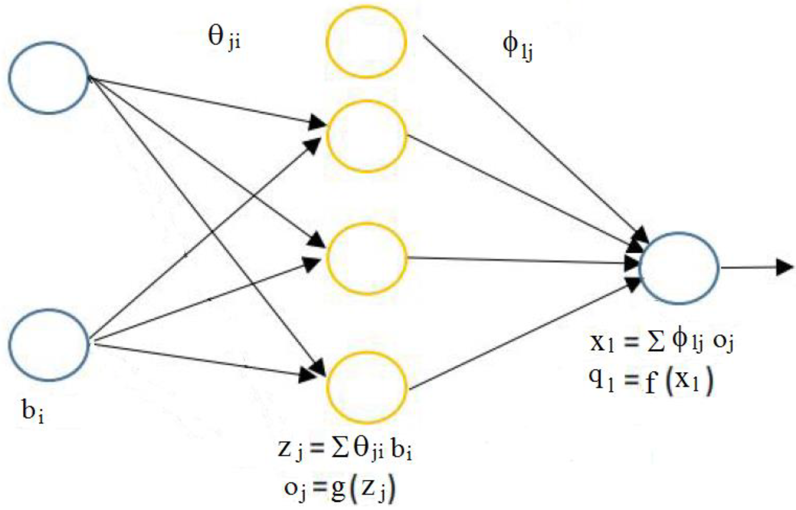
2. The Hessian for Neural Network Tuning

The algorithms for neural network tuning frequently evaluate the first derivatives of the cost map with respect to the scale parameters. Nevertheless, there are several cases where it is interesting to get the second derivatives of the cost map with respect to the scale parameters. The second derivatives of the cost map with respect to the scale parameters are known as the Hessian.

2.1. Design of the Hessian

In this article, we utilize a neural network with only one hidden layer. It could be expanded to a multilayer neural network, but in this article, we utilize a small neural network. This neural network utilizes sigmoid maps in the hidden layer and a linear map in the output layer. We express the neural network as
q l = j φ l j g ( i θ j i b i )
where θ j i is the scale parameter of the hidden layer, φ l j is the scale parameter of the output layer, g is the activation map, b i are the inputs, and q l are the outputs.
We take into account the neural network in Figure 1 where n is the input layer, l is the hidden layer, and m is the output layer. We express the scale parameters from the input layer to the hidden layer as θ j i and the scale parameters from the hidden layer to the output layer as θ l m .
We express the cost map as
E = 1 2 l = 1 L T ( q l t l ) 2
where q l is the output of the neural network and t l is the target, L T is the total output number. We express the forward propagation as
z j = i θ j i b i o j = g ( z j ) x l = j φ l j o j q l = f ( x l ) = x l
where b i is the input, q l is the output of the neural network, θ j i are hidden layer scale parameters, and φ l j are output layer scale parameters.
We take into account the activation map in the hidden layer as
g ( z j ) = 1 1 + e z j .
The first and second derivatives of the sigmoid map (4) are
g / ( z j ) = g ( z j ) ( 1 g ( z j ) ) , g / / ( z j ) = g ( z j ) ( 1 g ( z j ) ) ( 1 2 g ( z j ) ) .
We take into account the activation map of the output layer as the linear form
f ( x l ) = x l .
The first and second derivatives of the linear map (6) are
f / ( x l ) = 1 , f / / ( x l ) = 0 .
The first and second derivatives of the cost map (2) are
E q l = ( q l t l ) , 2 E q l 2 = 1 .
Using the cost map (2) and f ( x l ) = x l (6), we express the propagation of the output layer as
E φ l j = E q l q l x l x l φ l j = ( q l t l ) f ( x l ) x l o j = ( q l t l ) x l x l o j = ( q l t l ) ( 1 ) g ( z j ) , E φ l j = ( q l t l ) g ( z j ) .
Using the cost map (2) and g / ( z j ) = o j z j = g ( z j ) z j = g ( z j ) ( 1 g ( z j ) ) (5), we express the propagation of the hidden layer as
E θ j i = E q l q l x l x l o j o j z j z j θ j i = ( q l t l ) ( 1 ) φ l j g / ( z j ) b i , E θ j i = ( q l t l ) φ l j g ( z j ) ( 1 g ( z j ) ) b i .
We express the second derivative of E as the Hessian H :
H = E = 2 E θ 2 = [ 2 E θ j i 2 2 E θ j i φ l j 2 E θ j i φ l j 2 E θ φ l j 2 ]
and the Hessian is symmetrical:
2 E θ j i φ j l = 2 E φ j l θ j i .
The Hessian terms are
2 E θ j i 2 = b i b i T φ l j [ g / / ( z j ) σ i + g / ( z j ) 2 φ l j S i ] 2 E θ j i φ l j = b i g / ( z j ) [ σ i + o j φ l j S i ] 2 E φ l j 2 = o j o j T [ f / / ( x l ) σ i + f / ( x l ) 2 S i ]
and
S i = 2 E q l 2 = 1 , g / ( z j ) = g ( z j ) ( 1 g ( z j ) ) ,   f / ( x l ) = 1 , g / / ( z j ) = g ( z j ) ( 1 g ( z j ) ) ( 1 2 g ( z j ) ) ,   f / / ( x l ) = 0 , o j = x l φ l j = g ( z j ) ,   b i = z j θ j i = inputs , g ( z j ) = 1 1 + e z j ,   f ( x l ) = x l , σ i = ( q l t l ) .
We substitute (13) and (11); then the Hessian is
H = E = 2 E θ 2 = [ 2 E θ j i 2 2 E θ j i φ l j 2 E θ j i φ l j 2 E φ l j 2 ] 2 E θ j i 2 = b i b i T φ l j [ g ( z j ) ( 1 g ( z j ) ) ( 1 2 g ( z j ) ) ( q l t l ) + g ( z j ) 2 ( 1 g ( z j ) ) 2 φ l j ] 2 E θ j i φ l j = b i g ( z j ) ( 1 g ( z j ) ) [ ( q l t l ) + g ( z j ) φ l j ] 2 E φ l j 2 = g ( z j ) g ( z j ) T
where b i are the inputs, q l are the outputs, g ( z j ) = 1 1 + e z j are the activation maps, t l are the targets, z j = θ j i b i are the hidden layer outputs, and φ l j are the scale parameters of the hidden layer.
In the next step, we evaluate the Hessian using the Newton method.

2.2. Design of the Newton Method

It is necessary to express a method to tune the scale parameters of the Hessian. The Newton method is one alternative to tune the scale parameters of the Hessian. We express the basic tuning of the Newton method as follows:
[ θ j i , k + 1 φ l j , k + 1 ] = [ θ j i , k φ l j , k ] α H k 1 [ E k θ j i , k E k φ l j , k ] H k = [ 2 E k θ j i , k 2 2 E k θ j i , k φ l j , k 2 E k θ j i , k φ l j , k 2 E k φ l j , k 2 ]
where 2 E k θ j i , k 2 , 2 E k φ l j , k 2 , 2 E k θ j i , k φ l j , k are as in (14) for each k ; E k φ l j , k , E k θ j i , k are as in (9), (10); θ j i , k , φ l j , k are the scale parameters; and α is the tuning factor. The Newton method can quickly reach a minimum. The Newton method requires the existence of the inverse of the Hessian ( H k 1 ).
Now, we express the Newton method of (15) by terms. First, from (15), we obtain the inverse of H k as
H k 1 = [ 2 E k θ j i , k 2 2 E k θ j , k φ l j , k 2 E k θ j i , k φ l j , k 2 E k φ l j , k 2 ] 1 = { 1 ( 2 E k θ j i , k 2 ) ( 2 E k φ l j , k 2 ) ( 2 E k θ j i , k φ l j , k ) 2 * [ 2 E k φ l j , k 2 2 E k θ j i , k φ l j , k 2 E k θ j i , k φ l j , k 2 E k θ j i , k 2 ] } .
We substitute H k 1 of (16) and θ k , E k θ k of (16) into θ k + 1 of (16) as follows:
[ θ j i , k + 1 φ l j , k + 1 ] = [ θ j i , k φ l j , k ] { α 1 ( 2 E k θ j i , k 2 ) ( 2 E k φ l j , k 2 ) ( 2 E k θ j i , k φ l j , k ) 2 * [ 2 E k φ l j , k 2 2 E k θ j i , k φ l j , k 2 E k θ j i , k φ l j , k 2 E k θ j i , k 2 ] [ E k θ j i , k E k φ l j , k ] } .
We express (17) by terms as
θ j i , k + 1 = θ j i , k β H j i , k E k θ j i , k + γ H , k E k φ l j , k φ l j , k + 1 = φ l j , k β H l j , k E k φ l j , k + γ H , k E k θ j i , k β H j i , k = α 2 E k φ l j , k 2 ( 2 E k θ j i , k 2 ) ( 2 E k φ l j , k 2 ) ( 2 E k θ j i , k φ l j , k ) 2 β H l j , k = α 2 E k θ j i , k 2 ( 2 E k θ j i , k 2 ) ( 2 E k φ l j , k 2 ) ( 2 E k θ j i , k φ l j , k ) 2 γ H , k = α 2 E k θ j i , k φ l j , k ( 2 E k θ j i , k 2 ) ( 2 E k φ l j , k 2 ) ( 2 E k θ j i , k φ l j , k ) 2
where 2 E k θ j i , k 2 , 2 E k φ l j , k 2 , 2 E k θ j i , k φ l j , k are as in (14) for each k ; E k φ l j , k , E k θ j i , k are as in (9), (10) for each k ; θ j i , k , φ l j , k are the scale parameters for each k ; and α is the tuning factor. Thus, (18) is the Newton method by terms.
For comparison, we express the steepest descent method as
θ j i , k + 1 = θ j i , k β G j i , k E k θ j i , k + γ G , k E k φ l j , k φ l j , k + 1 = φ l j , k β G l j , k E k φ l j , k + γ G , k E k θ j i , k β G j i , k = α β G l j , k = α γ G , k = 0
where E k φ l j , k , E k θ j i , k are as in (9), (10) for each k ; θ j i , k , φ l j , k are the scale parameters for each k ; and α is the tuning factor. Thus, (19) is the steepest descent method.
It can be seen that the Newton method by terms (Hessian) (18) has the same form as the steepest descent (19). However, the steepest descent (19) takes into account constant values in its tuning rate β G i j , k , β G j i , k and momentum γ G , k , while the Hessian (18) takes into account the second-order partial derivatives of the cost map with respect to the scale parameters in its tuning rate β H i j , k , β H j i , k and momentum γ H , k .
We express the mini-batches in the next section to get better tuning of the Hessian.

3. Mini-Batches to Get Better Tuning of the Hessian

The form to update the scale parameters of the neural networks is that each neuron assigns information to the next neuron and it receives information from the previous neuron. We need training for successful neural network tuning. The training is developed from one epoch to the next until the scale parameters reach constant values and the cost map reaches a minimum. In addition, we need the training data to be tuned in a random form with the goal to quickly reach a minimum.
In the training stage, the neural network computes its outputs each time to obtain a result, and we compare the outputs with targets; in this way, the cost map of the neural network decreases. The scale parameters take random initial values, and these scale parameters are tuned through time.
We use other testing data as the basic method to evaluate the neural network efficacy. This consists of taking 80 % of the data for training and taking 20 % of the data for testing. The first stage is the training, and the second stage is the testing.
In the tuning, the training and testing stages are important.

Design of the Mini-Batches

We take into account training data v and u characteristics:
B u v = [ b 1 , b 2 , b 3 , , b v ] b 1 , u v ,
Q v = [ q 1 , q 2 , q 3 , , q v ] q 1 , v .
In the mini-batches, we divide the training data v into w -many mini-batches of size y , with the goal to quickly reach a minimum.
B u v = [ | b u 1 , , b u y b 1 , u y | b u y + 1 , , b u 2 y b 2 , u y | , b u w y | b w , u y ]
Q v = [ | q 1 , , q y q 1 , y | q y + 1 , , q 2 y | q 2 , y , , q w y | q w , y ]
We express the Hessian with mini-batches as (we divide the training data v in w-many mini-batches of size y ):
(1)
For each epoch.
(2)
Evaluate the mini-batches and tune each of the mini-batches c = 1 , 2 , , w with (24). These values are expressed in (15), (18).
(3)
Repeat for the next epoch.
θ k + 1 = θ k α d = 1 y H k , d 1 E k , d θ k
We express the properties of the mini-batches below:
  • Most of the time, we do not need to utilize all data to reach an acceptable descent direction. A small number of mini-batches could be sufficient to estimate the target.
  • Obtaining the Hessian using all the training data could have high computational cost.
The neural network tuning is performed using the Hessian with mini-batches (15), (18) where 2 E k θ j i , k 2 , 2 E k φ l j , k 2 , 2 E k θ j i , k φ l j , k are as in (14); E k φ l j , k , E k θ j i , k are as in (9), (10); and θ j i , k , φ l j , k are the scale parameters. We tune the neural network with a tuning factor of α and l neurons in the hidden layer, and we use e epochs. In this kind of tuning, we divide the training data into mini-batches as in (22,23).

4. Comparisons

In this section, we compare steepest descent (SD), steepest descent with mini-batches (SDMB) from [9,10,11,12], the Hessian (H) from [17,18,19,20], and the Hessian with mini-batches (HMB) from this investigation for electrical demand prediction. The goal of these algorithms is that the neural network output q l must reach the target t l as soon as possible.
Efficient electrical demand prediction is critical for acceptable operations and planning with the intention of achieving profits. The load forecast influences a series of decisions, including the generators to be used for a given period, and influences the wholesale prices and the market prices in the electrical sector.
The training data used were a table with the history of electrical demand for each hour and temperature observations provided by the International Organization for Standardization (ISO) of Great Britain. The meteorological information includes the dry bulb temperature and the dew point. We took into account the data of the hourly electrical demand.
For the electrical demand prediction, we took into account eight characteristics to tune the neural network:
  • The dry bulb temperature;
  • The dew point;
  • Hour of the day;
  • Day of the week;
  • A mark indicating if this is a free or a weekend day;
  • Medium load of the past day;
  • The load of the same hour, in the past day;
  • Load of the same hour, the same day of the past week.
Further, we utilized the load of the same day as the target.
  • Using the training data ( 34800 × 8 ), we trained the neural network for electrical demand prediction. After the training stage of the neural network, we used 8770 datapoints for the testing for each characteristic, yielding a matrix with dimensions ( 8770 × 8 )
  • The neural network had three layers—one input layer, one hidden layer, and one output layer. The input layer had eight neurons, the hidden layer had six neurons, and the output layer had one neuron.
We obtained neural network tuning by using the Hessian with the following steps:
  • We initialized the scale parameters with random values between 0 and 1 ;
  • We obtained the forward propagation;
  • We obtained the cost map;
  • We obtained the back propagation;
  • We utilized the Hessian tuning.
To evaluate the tuning of the neural network, we employed the determination coefficient ( R 2 ), the mean absolute error ( M A E ), and the mean absolute percent error ( M A P E ), determined as follows:
R 2 = 1 l = 1 L T ( q l t l ¯ ) 2 l = 1 L T ( t l t l ¯ ) 2 M A E = l = 1 L T | q l t l | M A P E = 100 L T l = 1 L T | q l t l |
where q l is the neural network output, t l is the target, and t l ¯ is the mean of the target. R 2 generates values from 0 to 1 ; L T is the total output number. If a method provides good tuning, it has R 2 values near to 1 , and if a method provides bad tuning, it has R 2 values near to 0 . If a method provides good tuning, it has M A E values near to 0 MWh, and if a method provides good tuning, it has M A P E values near to 0 % . We also used the cost map E (2) to evaluate the tuning of the neural network. If a method provides good tuning, it has E values near to 0 .

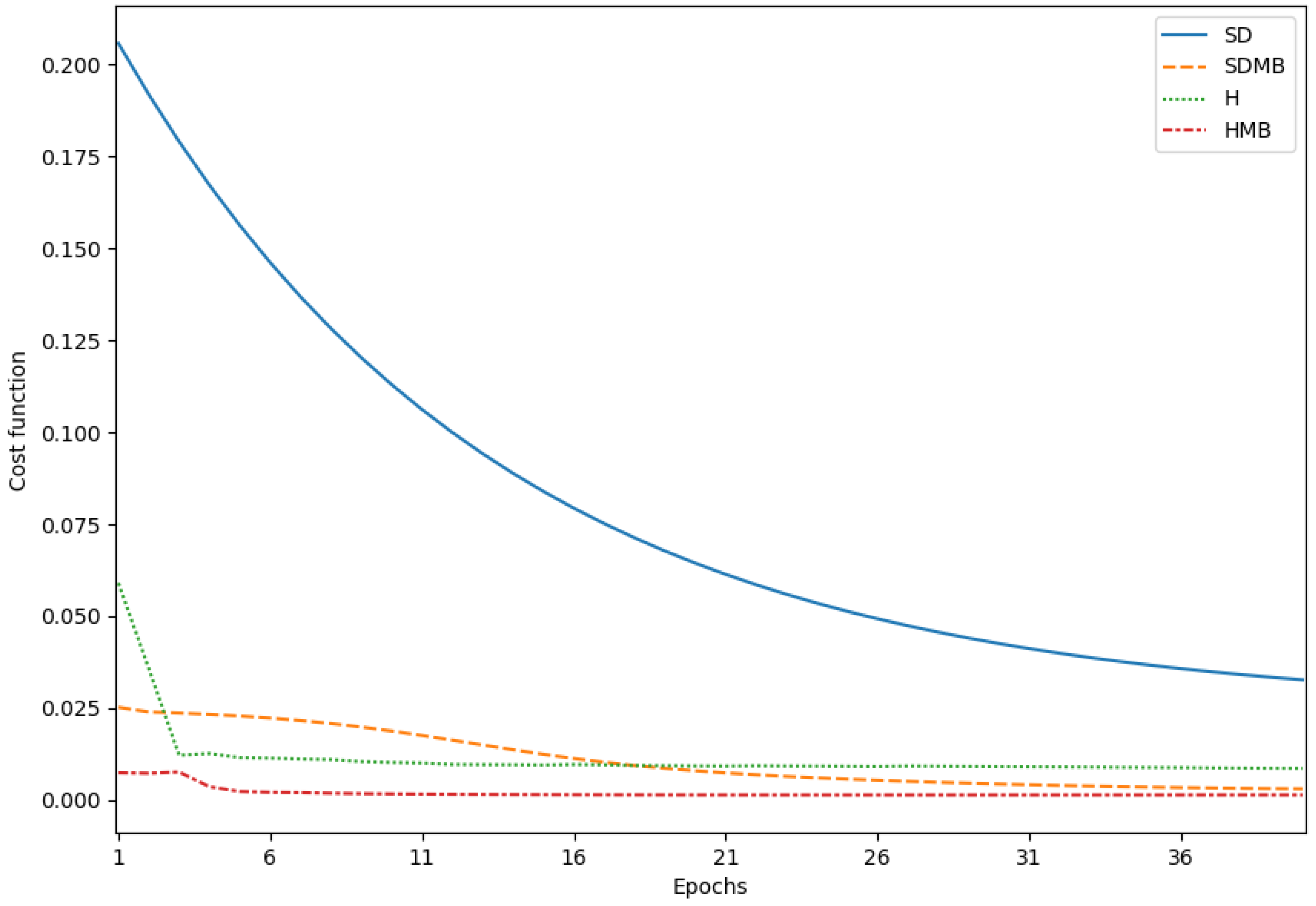
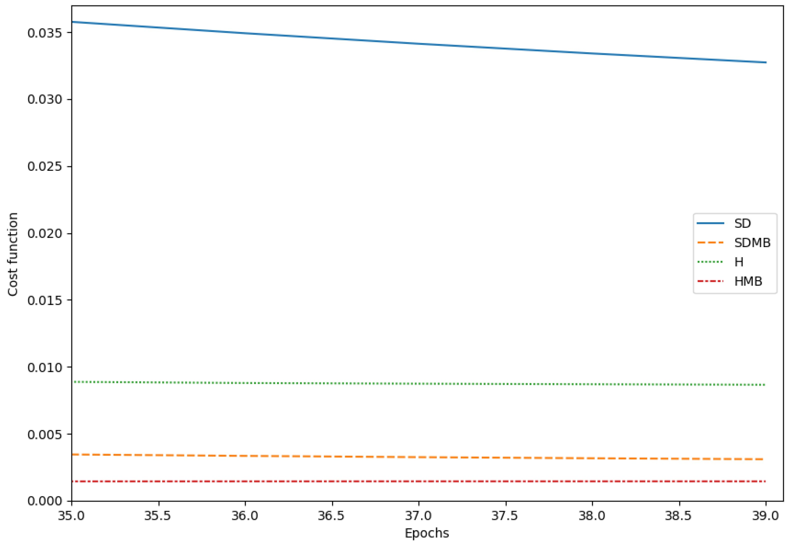
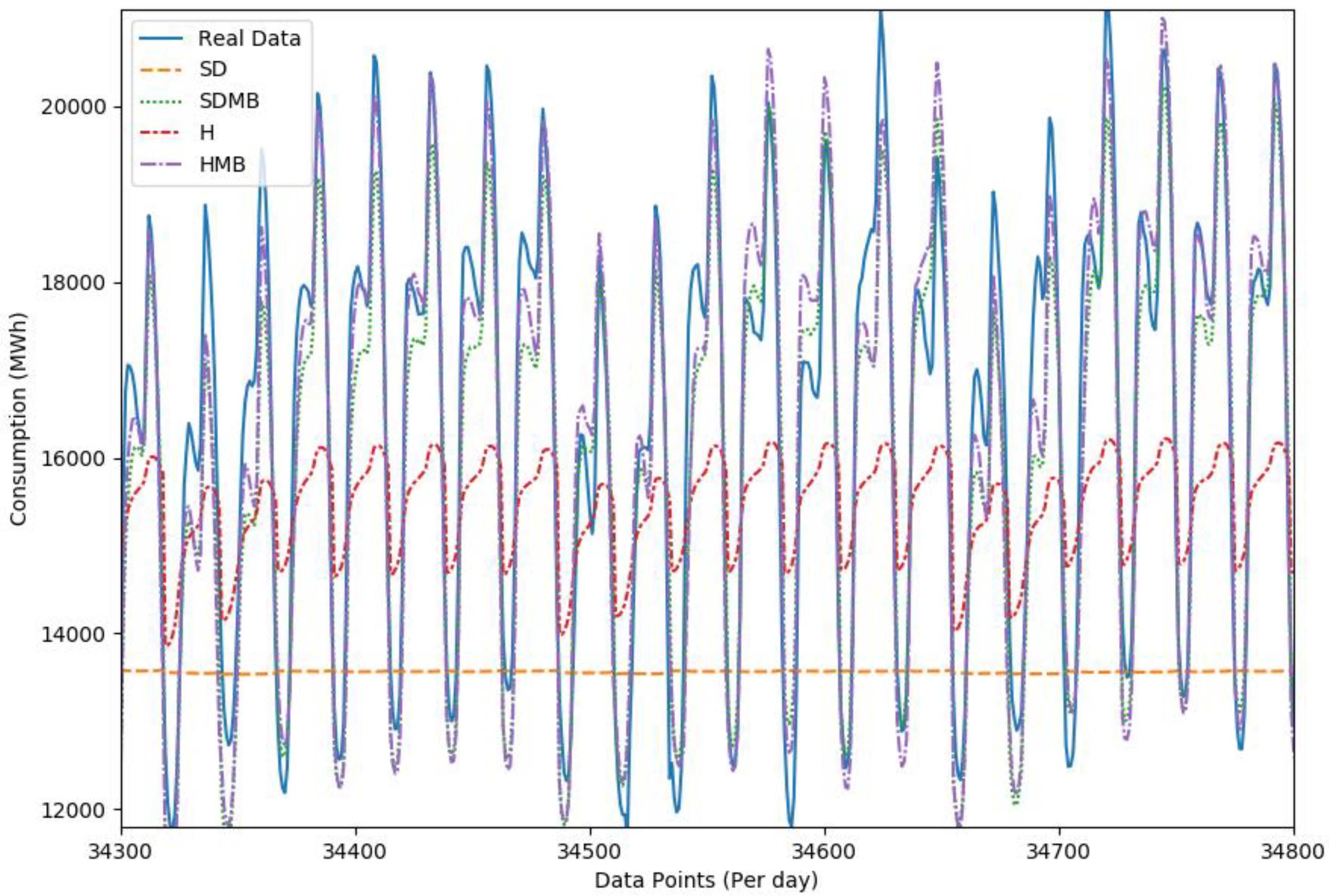
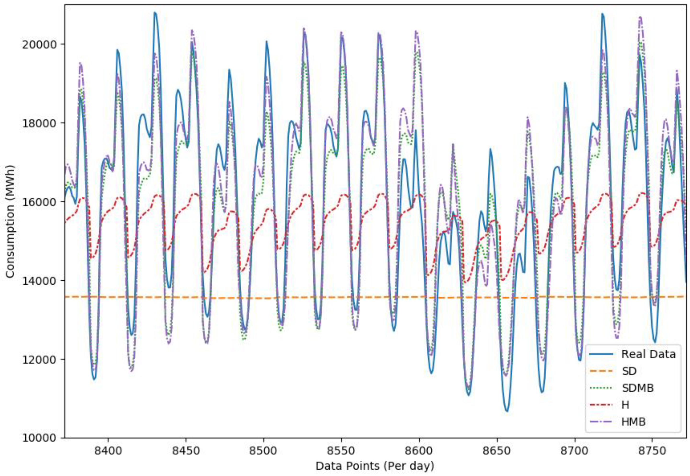
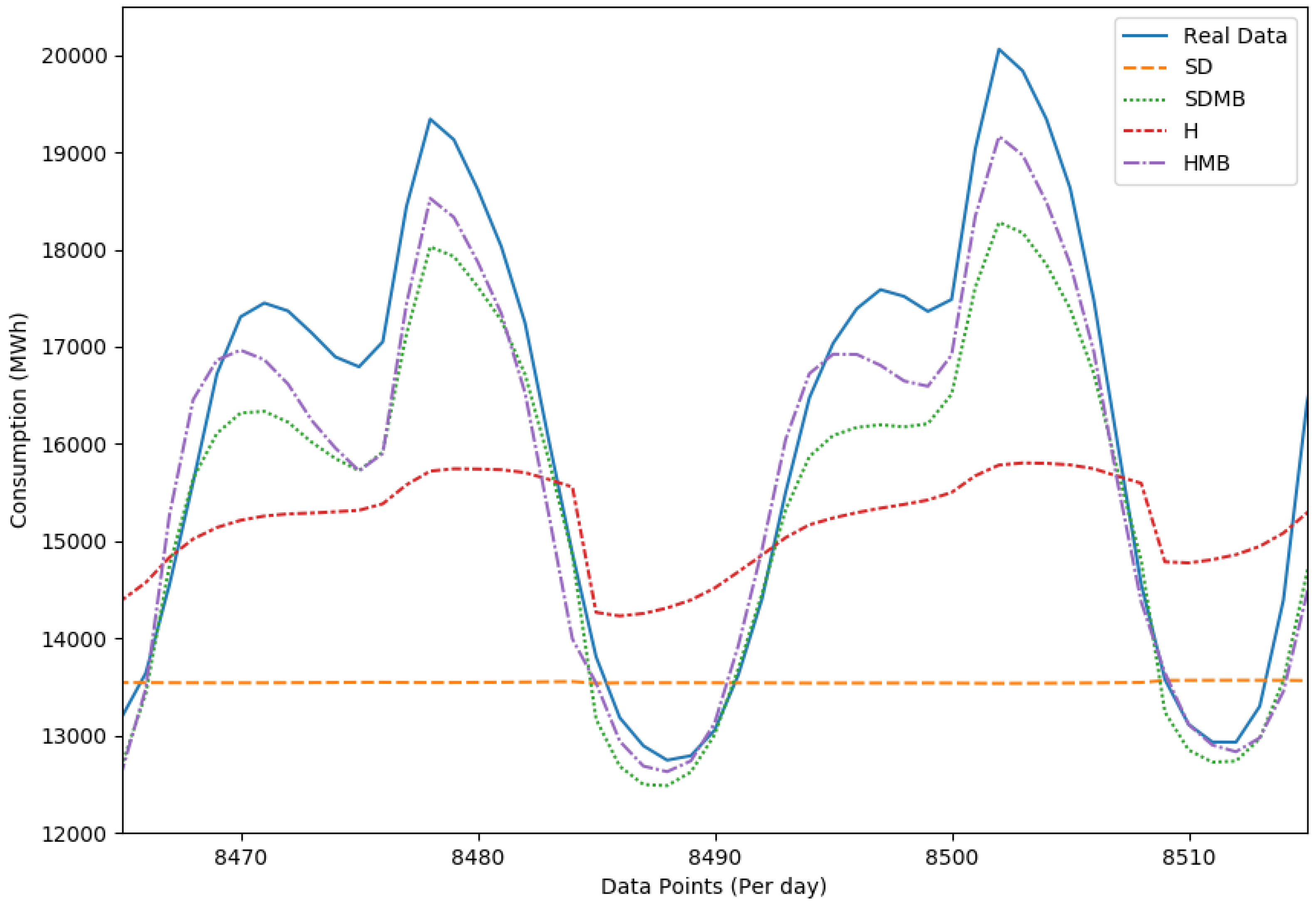
Results of the Comparison

It should be noted that the neural network trained by steepest descent (SD) (19) had l = 6 neurons in its hidden layer, a tuning factor of α = 0.0004 , and a number of epochs of e = 40 .
It should be noted that the neural network trained by steepest descent with mini-batches (SDMB) in [9,10,11,12] and using (19), (22), (23) had l = 6 neurons in its hidden layer, mini-batches with a size of y = 32 , a tuning factor of α = 0.0004 , and a number of epochs of e = 40 .
It should be noted that the neural network trained by the Hessian (H) in [17,18,19,20] and using (15), (18), (14), (9), (10) had l = 6 neurons in its hidden layer, a tuning factor of α = 0.0004 , and a number of epochs of e = 40 .
It should be noted that the neural network trained by the Hessian with mini-batches (HMB) in this investigation and using (15), (18), (14), (9), (10), (22), (23) had l = 6 neurons in its hidden layer, mini-batches with a size of y = 32 , a tuning factor of α = 0.0004 , and a number of epochs of e = 40 .
Figure 2 shows the cost maps during the training of the neural network with steepest descent (SD), steepest descent with mini-batches (SDMB), Hessian (H), and Hessian with mini-batches (HMB). As we can see, the Hessian with mini-batches provides better tuning when it comes to training the neural network and tends to converge more directly (with the help of the information provided from the second derivative) than with the use of the steepest descent. The issue with the normal downward steepest descent is that often a minimum cannot be quickly found. The use of mini-batches helps to quickly reach a minimum.
Figure 3 shows a zoom of the cost maps after 40 epochs during neural network training using SD, SDMB, H, and HMB. The Hessian provides better tuning in comparison with steepest descent, and the Hessian with mini-batches provides better tuning in comparison with steepest descent with mini-batches.
The tuning of the neural network with SD, SDMB, H, and HMB during training is shown in Figure 4. During 40 epochs, the neural network trained with steepest descent failed to tune, and its tuning was very slow when compared to the neural network trained with Hessian and mini-batches, which provided better tuning. The Hessian provided better tuning than steepest descent.
The neural network tuning using SD, SDMB, H, and HMB during testing is shown in Figure 5. Similar to the training results, the neural network trained using steepest descent did not have the ability to predict. The neural network prediction using the Hessian with mini-batches was better than that using the other methods, as can be seen in Figure 6, which is a zoom of the neural network prediction with SD, SDMB, H, and HMB during testing.
Table 1 compares the results of SD, SDMB, H, and HMB during training and testing with 40 epochs in terms of the determination coefficient ( R 2 ) and cost ( E ). It should be noted that the neural network had 6 neurons in its hidden layer and each mini-batch had a size of y = 32 .
R 2 has values between 0 and 1 , where values close to 1 correspond to algorithms with better tuning. Since HMB obtained the biggest value of R 2 during training and testing and obtained the smallest value of E during training, HMB provides the best tuning in comparison with H, SDMB, and SD.
Table 2 compares the results of SD, SDMB, H, and HMB during training and testing for 40 epochs in terms of the mean absolute error ( M A E ) and the mean absolute percent error ( M A P E ).
Smaller values of M A E and M A P E correspond to algorithms with better tuning. Since HMB obtained the smallest values of the M A E and M A P E during testing, HMB provides the best tuning in comparison with H, SDMB, and SD.
As we decrease the mini-batch size, we speed up the training of the algorithm, but we also increase the computation cost. This means a trade-off between computation cost and training speed.

5. Conclusions

Our goal in this article was to design the Hessian with mini-batches to get better tuning than steepest descent for a neural network. The Hessian with mini-batches was compared with steepest descent, steepest descent with mini-batches, and the Hessian for electrical demand prediction; since we reached the nearest approximation between the neural network output and the target and reached the smallest value of the cost map using the proposed algorithm, we got the best tuning with our proposed algorithm. In future work, we will find the convergence of the Hessian with mini-batches, we will propose other algorithms different to the Hessian to compare our results, and we will apply our algorithm for the prediction of other processes.

Author Contributions

Investigation and formal analysis I.E., J.d.J.R., D.R.C., and G.O.; software and validation J.F.N., D.I.M., and S.M.; writing—original draft, review and editing R.B., E.G., and C.F.J. All authors have read and agreed to the published version of the manuscript.

Funding

This research received no external funding.

Acknowledgments

The authors are grateful to the Guest Editors and reviewers for their valuable comments and insightful suggestions, which helped to improve this research significantly. The authors thank the Instituto Politécnico Nacional, Secretaría de Investigación y Posgrado, Comisión de Operación y Fomento de Actividades Académicas, and Consejo Nacional de Ciencia y Tecnología for their help in this research.

Conflicts of Interest

The authors declare no conflict of interest.

References

  1. Sadiq, M.; Shi, D.; Guo, M.; Cheng, X. Facial Landmark Detection via Attention-Adaptive Deep Network. IEEE Access 2019, 7, 181041–181050. [Google Scholar] [CrossRef]
  2. Wang, C.; Yao, H.; Liu, Z. An efficient DDoS detection based on SU-Genetic feature selection. Clust. Comput. 2019, 22, S2505–S2515. [Google Scholar] [CrossRef]
  3. Dinculeana, D.; Cheng, X. Vulnerabilities and Limitations of MQTT Protocol Used between IoT Devices. Appl. Sci. 2019, 9, 848. [Google Scholar] [CrossRef] [Green Version]
  4. Shi, F.; Chen, Z.; Cheng, X. Behavior Modeling and Individual Recognition of Sonar Transmitter for Secure Communication in UASNs. IEEE Access 2020, 8, 2447–2454. [Google Scholar] [CrossRef]
  5. Jia, B.; Hao, L.; Zhang, C.; Chen, D. A Dynamic Estimation of Service Level Based on Fuzzy Logic for Robustness in the Internet of Things. Sensors 2018, 18, 2190. [Google Scholar] [CrossRef] [PubMed] [Green Version]
  6. Wang, C.; Yang, L.; Wu, Y.; Wu, Y.; Cheng, X.; Li, Z.; Liu, Z. Behavior Data Provenance with Retention of Reference Relations. IEEE Access 2018, 6, 77033–77042. [Google Scholar] [CrossRef]
  7. Chen, Y.; Luo, F.; Li, T.; Xiang, T.; Liu, Z.; Li, J. A Training-integrity Privacy-preserving Federated Learning Scheme with Trusted Execution Environment. Inf. Sci. 2020, 522, 69–79. [Google Scholar] [CrossRef]
  8. Jia, B.; Xu, H.; Liu, S.; Li, W. A High Quality Task Assignment Mechanism in Vehicle-Based Crowdsourcing Using Predictable Mobility Based on Markov. IEEE Access 2018, 6, 64920–64926. [Google Scholar] [CrossRef]
  9. Cheng, F.; Zhang, X.; Zhang, C.; Qiu, J.; Zhang, L. An adaptive mini-batch stochastic gradient method for AUC maximization. Neurocomputing 2018, 318, 137–150. [Google Scholar] [CrossRef]
  10. Konecny, J.; Liu, J.; Richtarik, P.; Takac, M. Mini-Batch Semi-Stochastic Gradient Descent in the Proximal Setting. IEEE J. Sel. Top. Signal Process. 2016, 10, 242–255. [Google Scholar] [CrossRef]
  11. Vakhitov, A.; Lempitsky, V. Learnable Line Segment Descriptor for Visual SLAM. IEEE Access 2019, 7, 39923–39934. [Google Scholar] [CrossRef]
  12. Yang, H.; Jia, J.; Wu, B.; Gao, J. Mini-batch optimized full waveform inversion with geological constrained gradient filtering. J. Appl. Geophys. 2018, 152, 9–16. [Google Scholar] [CrossRef]
  13. Peng, K.; Leung, V.C.M.; Huang, Q. Clustering Approach Based on Mini Batch Kmeans for Intrusion Detection System Over Big Data. IEEE Access 2018, 6, 11897–11906. [Google Scholar] [CrossRef]
  14. Tang, R.; Fong, S. Clustering big IoT data by metaheuristic optimized mini-batch and parallel partition-based DGC in Hadoop. Future Gener. Comput. Syst. 2018, 86, 1395–1412. [Google Scholar] [CrossRef]
  15. Yang, Z.; Wang, C.; Zang, Y.; Li, J. Mini-batch algorithms with Barzilai-Borwein update step. Neurocomputing 2018, 314, 177–185. [Google Scholar] [CrossRef]
  16. Yang, Z.; Wang, C.; Zhang, Z.; Li, J. Random Barzilai-Borwein step size for mini-batch algorithms. Eng. Appl. Artif. Intell. 2018, 72, 124–135. [Google Scholar] [CrossRef]
  17. Krishnasamy, G.; Paramesran, R. Hessian semi-supervised extreme learning machine. Neurocomputing 2016, 207, 560–567. [Google Scholar] [CrossRef]
  18. Liu, W.; Ma, T.; Tao, D.; You, J. HSAE: A Hessian regularized sparse auto-encoders. Neurocomputing 2016, 187, 59–65. [Google Scholar] [CrossRef]
  19. Liu, W.; Liu, H.; Tao, D. Hessian regularization by patch alignment framework. Neurocomputing 2016, 204, 183–188. [Google Scholar] [CrossRef]
  20. Xu, D.; Xia, Y.; Mandic, D.P. Optimization in Quaternion Dynamic Systems: Gradient, Hessian, and Learning Algorithms. IEEE Trans. Neural Netw. Learn. Syst. 2016, 27, 249–261. [Google Scholar] [CrossRef] [Green Version]
  21. Annunziata, R.; Garzelli, A.; Ballerini, L.; Mecocci, A.; Trucco, E. Leveraging Multiscale Hessian-Based Enhancement with a Novel Exudate Inpainting Technique for Retinal Vessel Segmentation. IEEE J. Biomed. Health Inform. 2016, 20, 1129–1138. [Google Scholar] [CrossRef] [PubMed]
  22. Goncalves, L.; Novo, J.; Campilho, A. Hessian based approaches for 3D lung nodule segmentation. Expert Syst. Appl. 2016, 61, 1–15. [Google Scholar] [CrossRef]
  23. Rodrigues, L.C.; Marengoni, M. Segmentation of optic disc and blood vessels in retinal images using wavelets, mathematical morphology and Hessian-based multi-scalefiltering. Biomed. Signal Process. Control 2017, 36, 39–49. [Google Scholar] [CrossRef]
  24. Zhang, J.; Wan, Y.; Chen, Z.; Meng, X. Non-negative and local sparse coding based on l 2 -norm and Hessian regularization. Inf. Sci. 2019, 486, 88–100. [Google Scholar] [CrossRef]
  25. Attouch, H.; Peypouquet, J.; Redont, P. Fast convex optimization via inertial dynamics with Hessian driven damping. J. Differ. Equ. 2016, 261, 5734–5783. [Google Scholar] [CrossRef] [Green Version]
  26. Mesri, Y.; Khalloufi, M.; Hachem, E. On optimal simplicial 3D meshes for minimizing the Hessian-based errors. Appl. Numer. Math. 2016, 109, 235–249. [Google Scholar] [CrossRef]
  27. Petra, C.G.; Qiang, F.; Lubin, M.; Huchette, J. On efficient Hessian computation using the edge pushing algorithm in Julia. Optim. Methods Softw. 2018, 33, 1010–1029. [Google Scholar] [CrossRef]
  28. Xu, P.; Roosta, F.; Mahoney, M.W. Newton-typemethods for non-convex optimization under inexact Hessian information. Math. Program. 2019. [Google Scholar] [CrossRef] [Green Version]
  29. Feng, G.; Liu, W.; Li, S.; Tao, D.; Zhou, Y. Hessian-Regularized Multitask Dictionary Learning for Remote Sensing Image Recognition. IEEE Geosci. Remote Sens. Lett. 2019, 16, 821–825. [Google Scholar] [CrossRef]
  30. Liu, W.; Liu, H.; Tao, D.; Wang, Y.; Lu, K. Multiview Hessian regularized logistic regression for action recognition. Signal Process. 2015, 110, 101–107. [Google Scholar] [CrossRef] [Green Version]
  31. Ng, C.C.; Yap, M.H.; Costen, N.; Li, B. Wrinkle Detection Using Hessian Line Tracking. IEEE Access 2015, 3, 1079–1088. [Google Scholar] [CrossRef] [Green Version]
  32. Shi, C.; An, G.; Zhao, R.; Ruan, Q.; Tian, Q. Multiview Hessian Semisupervised Sparse Feature Selection for Multimedia Analysis. IEEE Trans. Circuits Syst. Video Technol. 2017, 27, 1947–1961. [Google Scholar] [CrossRef]
  33. Liu, P.; Xiao, L. A Novel Generalized Intensity-Hue-Saturation (GIHS) Based Pan-Sharpening Method with Variational Hessian Transferring. IEEE Access 2019, 7, 39923–39934. [Google Scholar] [CrossRef]
  34. Zhang, Y.; Zhang, N.; Sun, D.; Toh, K.C. An efficient Hessian based algorithm for solving large-scale sparse group Lasso problems. Math. Program. 2018, 179, 223–263. [Google Scholar] [CrossRef] [Green Version]
  35. Feng, G.; Liu, W.; Tao, D.; Zhou, Y. Hessian Regularized Distance Metric Learning for People Re-Identification. Neural Process. Lett. 2019, 50, 2087–2100. [Google Scholar] [CrossRef]
  36. Zhu, C.; Gates, D.A.; Hudson, S.R.; Liu, H.; Xu, Y.; Shimizu, A.; Okamura, S. Identification of important error fields in stellarators using the Hessian matrix method. Nucl. Fusion 2019, 59, 1–13. [Google Scholar] [CrossRef] [Green Version]
  37. Quirynena, R.; Houska, B.; Diehl, M. Efficient symmetric Hessian propagation for direct optimal control. J. Process Control 2017, 50, 19–28. [Google Scholar] [CrossRef] [Green Version]
  38. Sun, T.; Yang, S. An Approach to Formulate the Hessian Matrix for Dynamic Control of Parallel Robots. IEEE/ASME Trans. Mechatron. 2019, 24, 271–281. [Google Scholar] [CrossRef]
Figure 1. The neural network.
Applsci 10 02036 g001
Figure 2. The cost maps during training, steepest descent (SD), steepest descent with mini-batches (SDMB), Hessian (H), Hessian with mini-batches (HMB).
Applsci 10 02036 g002
Figure 3. A zoom of the cost maps after 40 epochs during training.
Applsci 10 02036 g003
Figure 4. The neural network with the algorithms during training.
Applsci 10 02036 g004
Figure 5. The neural network with the algorithms during testing.
Applsci 10 02036 g005
Figure 6. A zoom of the neural network with the algorithms during testing.
Applsci 10 02036 g006
Table 1. Comparison results in terms of R 2 and cost ( E ).
R 2 (Training) R 2 (Testing) E (Training)
SD0.3060.1070.032
SDMB0.8750.8910.0031
H0.2980.2570.0086
HMB0.8820.8970.0014
Table 2. Comparison results in terms of mean absolute error ( M A E ) and mean absolute percent error ( M A P E ).
M A E (Testing) M A P E (Testing)
SD2396.78 MWh16.54%
SDMB699.39 MWh4.85%
H1888.61 MWh14.50%
HMB681.42 MWh4.77%

