Voting-Based Document Image Skew Detection
by
 , ,
, ,
Costin-Anton Boiangiu
1,* ,
,
Ovidiu-Alexandru Dinu
1,
Cornel Popescu
1 ,
,
Nicolae Constantin
2 and
Cătălin Petrescu
2 1
Computer Science and Engineering Department, Faculty of Automatic Control and Computers, Politehnica University of Bucharest, Splaiul Independenței 313, 060042 Bucharest, Romania
2
Automatic Control and Systems Engineering Department, Faculty of Automatic Control and Computers, Politehnica University of Bucharest, Splaiul Independenței 313, 060042 Bucharest, Romania
*
Author to whom correspondence should be addressed.
Appl. Sci. 2020, 10(7), 2236; https://doi.org/10.3390/app10072236
Submission received: 20 February 2020
/
Revised: 16 March 2020
/
Accepted: 24 March 2020
/
Published: 25 March 2020
(This article belongs to the Section Computing and Artificial Intelligence)
Abstract
:Optical Character Recognition (OCR) is an indispensable tool for technology users nowadays, as our natural language is presented through text. We live under the need of having information at hand in every circumstance and, at the same time, having machines understand visual content and thus enable the user to be able to search through large quantities of text. To detect textual information and page layout in an image page, the latter must be properly oriented. This is the problem of the so-called document deskew, i.e., finding the skew angle and rotating by its opposite. This paper presents an original approach which combines various algorithms that solve the skew detection problem, with the purpose of always having at least one to compensate for the others’ shortcomings, so that any type of input document can be processed with good precision and solid confidence in the output result. The tests performed proved that the proposed solution is very robust and accurate, thus being suitable for large scale digitization projects.
1. Introduction
Whenever documents are manually scanned, a human-made orientation error almost always occurs, preventing the Optical Character Recognition (OCR) engine from properly detecting the scanned content. Thus, we can say that almost all documents that are manually scanned are also skewed.
The problem of skew detection and correction is not a new one [1]. In order to ensure a correct layout analysis of image documents, or to have a high accuracy in the OCR process output, the input images must be skew free, otherwise the rows and columns (in the case of multi-column documents) might not be detected properly [2].
There have been numerous attempts to solve the deskew [3] problem, occasionally accompanied by text orientation detection [4,5]. The proposed approaches range from projection profiling [6], neighborhood clustering [7,8], Hough transform applied on different selected key-points [9,10,11], Fast Fourier Transform (FFT) [12], Principal Component Analysis (PCA) [13], Radon transform [14], vertical projections [15], morphology [16], machine learning approaches [17], etc. They obtain robust and accurate results in most cases considering that the elements and properties they try to detect and measure are present in the input image. However, this is not always the case. Projection profiling and neighborhood clustering need consistent lines of paragraph-like text, the former working best in single-column layouts. They do not work well if significant chunks of text are not available. Hough transform may well detect table-like structures and baseline dominant text orientation. If tables or line-like separators are not present and the available text is not bottom-aligned, this method will fail or, even worse, will return erroneous results. FFT may assist in obtaining a dominant alignment angle in the input image, no matter what the content of the image is, but its uptime is no better than the aforementioned methods. The main idea that derives from here is that one can develop a voting scheme using multiple experts’ decisions and confidence values [18,19,20], thus compensating the shortcomings or erroneous decisions of one approach with the benefits of another.
The current paper aims to offer an application-oriented, practical solution with a robust real-world behavior and not just a general framework, theoretically-oriented, based on multiple experts’ decision, alternative for classical approaches. Three skew detection algorithms were chosen to cover all the facets of the skew-related problems: the difficulty of finding the text orientation due to the shortage of aligned texts, the difficulty in finding lines and tables which may guide in finding the correct skew, the difficulty in understanding the image at all (thus the need to analyze it in the frequency domain instead of the value domain) and not just to exemplify the superiority of a voting-based decision mechanism over an independent decision.
This paper presents an approach to deskewing documents, designed for general purpose use, for generic documents that contain different text or geometrical features that may be used in finding a correct orientation. We combine the outputs of three different algorithms, each one also outputting a confidence measure in its work. The confidence is used to characterize the candidate for the voting, the skew angle result computed by each algorithm. The effect of having algorithms of various classes which operate on different aspects of the input image is that the winner algorithm compensates for the shortcomings of the other two. An aggregate confidence of the entire solution is also provided, so that it may be fully integrated into a real-world, mass production digital content producer application.
We will consider that the absolute value of the skew angle will never exceed 10°, or else the document is skewed on purpose. It can be any value, as we do not need this limitation in order for the algorithms to work, but doing this considerably saves execution time. So, we will refer the Skew Angle Search Space (SASS) to be the interval [−10°, 10°].
2. Skew Detection Algorithms
We present three approaches to detect skew, first making use of the frequency domain, and the other two using spatial domain exclusively.
2.1. Frequency Domain
2.1.1. Mechanism
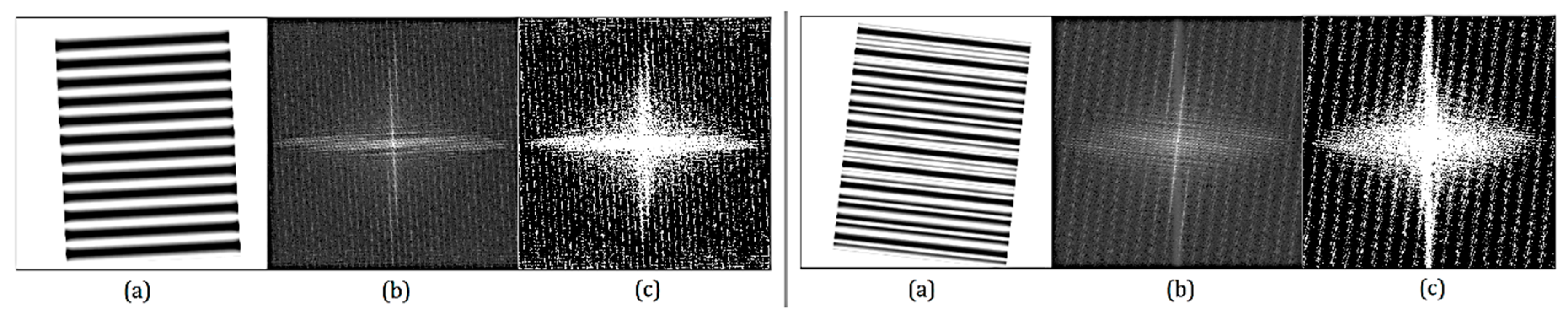
For tilted pages, near-vertical and near-horizontal lines occur in the frequency domain, due to the definition of the Fourier Transform and because text documents are composed of mostly vertical and horizontal sinusoids.
For an image which contains stripes, the Fast Fourier Transform (FFT) [21] yields points which align in a straight line, passing through the center of the FFT image and perpendicular to the stripes, as shown in Figure 1.
Lines in the frequency domain emerge from the patterns of parallel lines of text and horizontal/vertical separators, including whitespace. The angles of these lines lead to the document skew angle.
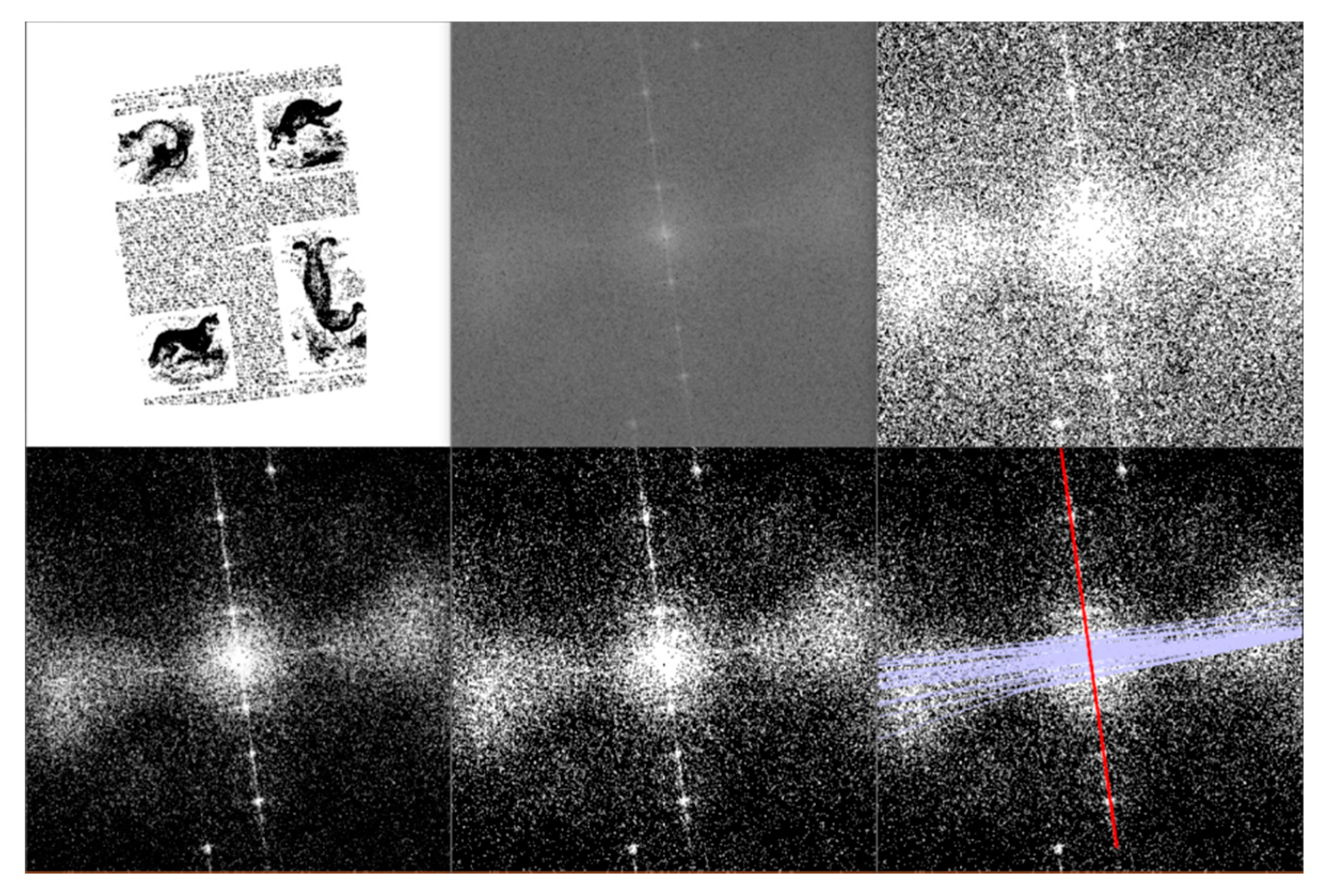
The FFT image is binarized with Otsu [22] and then the Hough transform [23] is applied to detect the dominant lines. Only lines that pass through the center of the FFT image are of interest. The skew angle is calculated as the angle between each dominant line and the closest axis. A weighted sum of these lines is then returned. The vertical line represents horizontal stripes in the input image, which is the information of the text rows, and the horizontal line represents vertical separators, including whitespace.
2.1.2. Improvements
The FFT image presents the challenge of detecting the dominant lines which represent the document orientation. It is noisy because of the high-frequency signals generated by text, small symbols spread across the whole document, images, etc. The FFT image also lacks contrast. These two shortcomings make it difficult for the Hough transform to identify the dominant lines which give the document orientation.
We solved these issues by stretching the contrast of the FFT image and then equalizing its histogram, before Otsu binarization and then feeding it to the Hough transform procedure. These operations help the binarization to emphasize dominant lines.
We have experimented with various methods of emphasizing the correct dominant lines by processing both the input image and the FFT image. Empirically, we have come to the conclusion that there is no need to process the input image in the spatial domain, as its FFT already contains all the orientation information, visually. Altering it only decays the dominant lines in the frequency domain. So, we only processed the FFT image.
Due to the noise in the FFT image, despite losing information in the input image, we initially tried blurring in the spatial domain in order to filter out high frequencies, but quickly discarded it as it produces fainter dominant lines in the frequency domain. Dilation [24] of the page content also produces incomplete lines on the FFT. These make the binarization produce gaps in the dominant lines and make it impossible to detect them using Hough transform.
Then we experimented with blurs in the frequency domain (namely Gaussian blur, box blur, bilateral filter, and median filter [25]), before binarization, and they partially worked, but none turned out to be nearly as feasible as contrast stretching followed by histogram equalization, and even when used together with these two, blurs do not improve accuracy.
In Figure 2, we present the result of contrast stretching and histogram equalization.
2.1.3. Confidence
We define a confidence metric (Equation (1)), which depends on the detected dominant lines’ strength in an FFT image I. The absolute value of the difference between two parameters: the mean color of all pixels L within some fixed distance range from the dominant line, and the mean color of the rest of the image, I\L, the complement of L. We consider black to be zero and white to be one, so the confidence is also between zero and one. The obtained measure is fine-tuned by being raised to some positive exponent , since a balance between all algorithms’ confidences will be enforced by employing a power–law relation, and their corresponding will be chosen to ensure equal average success confidence (i.e., excluding confidence in failure cases).
2.1.4. Projection Profiling Variant
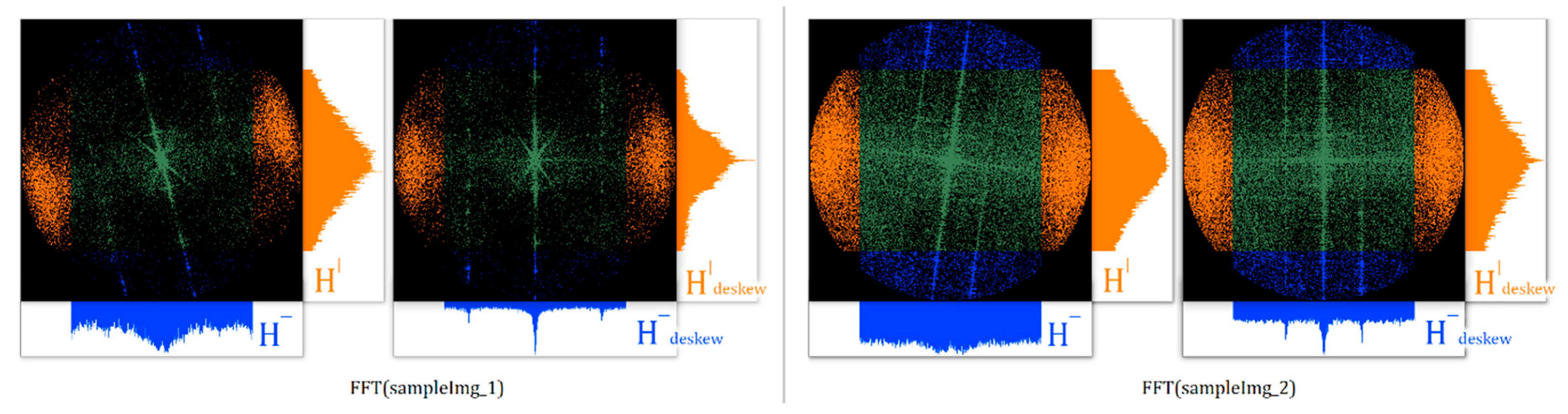
Instead of doing line detection with the Hough transform on the FFT image, we found the skew angle via the maximization of the variance in the projection space, as described in Section 2.2. We are interested in the variance with respect to both axes, centered in the middle of the FFT image. This is shown in Figure 3 with blue.
This alternative to the Hough line detection proves to be more stable, though the accuracy is approximately the same. Therefore, for both benchmarks and the fine-tuning exponent search, we used projection profiling in the frequency domain.
2.2. Projection Profiling Row Align
2.2.1. Mechanism
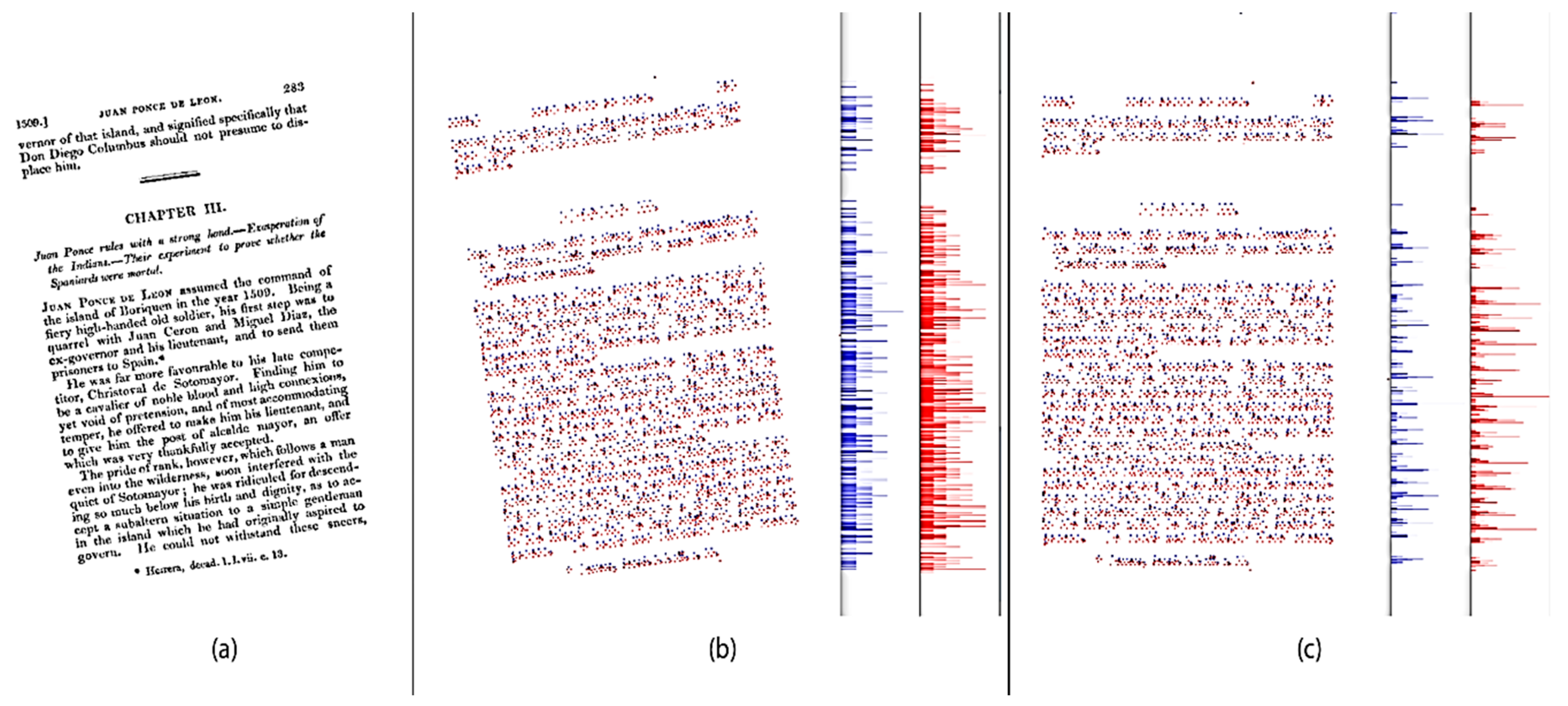
The projection profiling method [26] computes histograms on the vertical axis of the document, accumulating horizontal scanline black pixel count, assuming the text is black on white background. The algorithm swipes a scanline from the top to the bottom of the document, which writes the number of black pixels it contains in a buffer, at an index proportional to its current vertical position in the document.
We refer to this buffer as the histogram or the scanline pixel count buffer. Its size is fixed, is set by the user and is referred to as the histogram resolution.
The histogram will present the maximum variance when the text is skew-free, because of scanlines containing complete horizontal slices of lines of text (above the mean), and scanlines completely containing whitespace (completely below the mean). In other words, the skew angle is computed as the angle in the SASS which produces maximal scanline variance. The process is illustrated in Figure 4.
Variance of the histogram H of size N is given by the equation:
where is cycling through all connected components axis-aligned bounding boxes (AABBs), the number of top or bottom points that lie on the same horizontal scanline at a document height correspondent to position k in the histogram. As the resolution of H is fixed, k is not equal to the y coordinate of the points in document space. is the mean of H and is the angle by which the points are rotated.
2.2.2. Improvements
First, the image is binarized via standard bimodal Otsu thresholding.
Then, we find the connected components in the image and compute their axis-aligned bounding boxes (AABBs) [27]. The purpose is that we only try to align points of interest into horizontal rows, landmarks of connected components which represent text symbols.
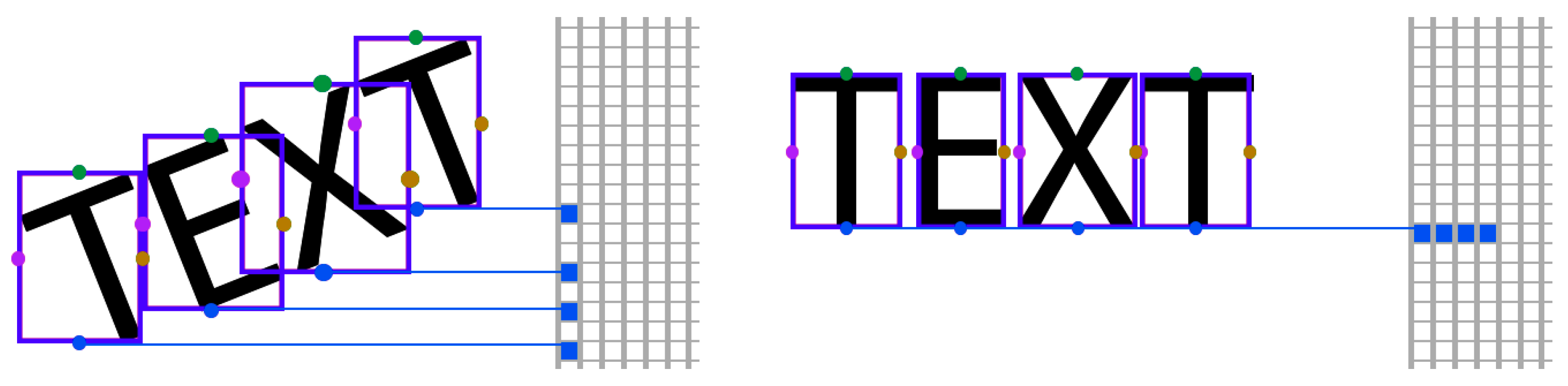
The top and bottom midpoints of the AABBs’ sides are the only points we need to rotate in order to find the skew angle. We illustrate the mechanism in Figure 5.
To avoid computation with elements that are not text symbols, we compute the average width and height of the AABBs. If an AABB of a connected component is considerably larger than this average, we discard it from the rotation phase, as it does not represent a text symbol, or does not belong to a block of text.
With a small step, such as a tenth of a degree, we compute the variance of the document’s bottom and top histograms for all angles in the SASS and pick the winner skew angle as the one which gives the greatest sum of the aforementioned variances.
It is unknown where the global maximum is for the document’s scanline variance as a function of an angle, so it is safest to search the whole SASS, rather than using some fast convergence heuristic like a binary search or gradient descent. Unlike them, the brute force search guarantees to find the global maximum. The search space contains 200 or 300 angle candidates, and the scanline variance for one angle is computed in less than 100 microseconds, which is due to the fact that we only rotate at most a couple of thousand points per iteration. Therefore, the brute force search is the most recommended approach here.
However, by sampling the variance for all angles in SASS, we are able to define a confidence metric, as described in Section 2.2.3.
2.2.3. Confidence
Let be the standard deviation of the variance function as discussed in Section 2.2.1. Let be the mean of the histogram variances for all . If is the angle which produces the maximum value of , namely , then we can define the confidence measure as follows:
As the denominator term represents the variance deviation for the found skew angle, we can see that as it increases, the confidence also increases. This is measuring how much of a difference the shift in the angle space has made for the variance when maximized it. is a positive exponent used for fine-tuning the confidence in the voting process to match the capabilities of the other algorithms.
2.3. Spatial Domain Lines
2.3.1. Mechanism
This method uses horizontal and vertical lines in the document detected via the Hough transform [28] to compute the skew angle. We look for both vertical and especially for horizontal lines, which are most likely to be detected within lines of text. The skew angle is computed as a weighted sum of angles given by the detected lines. For the summation, these angles are weighted by properties of the lines. The algorithm performs best when there are long lines in the document, such as tables and separators.
First, the Sobel [29] edge detection filter is applied, in order to empty the interior of the connected components. This prepares the image for the line detection procedure, eliminating shape filling pixels from being accounted in the line search procedure.
After we apply the probabilistic Hough transform, we are left with a set of line segments, each one representing some vertical or horizontal separator, some line of a table, some line in an image, a line of text, or some line emerging at a random angle from within the placement of the symbols, randomly cutting through a block of text. The former must have discarded, as it does not represent the orientation of the document. Thus, we must sort the obtained segments by some criteria. Lines outside SASS are discarded.
We take all pairs of segments and build an adjacency matrix which contains one in the cell [i,j] if line i and line j may be considered parallel and zero otherwise. Two lines are considered parallel if the absolute value of the dot product of their support unit vectors is greater than one minus some small threshold ε. The computed dot products are also saved in a matrix for later use.
We partition all segments into disjoint sets, each set containing lines claimed to be parallel, i.e., for any pair of lines within a set, the adjacency matrix has a value of 1. For this step, an optimized disjoint sets union-find data structure is used, with path compression for the find operation and union by size heuristics. For every resulting set of parallels, we compute an average line, referred to as the set representative, which gives the orientation of the set.
If all line segments are in one set, then the returned skew angle is equal to the angle between the representative line of the set and the closest primary axis.
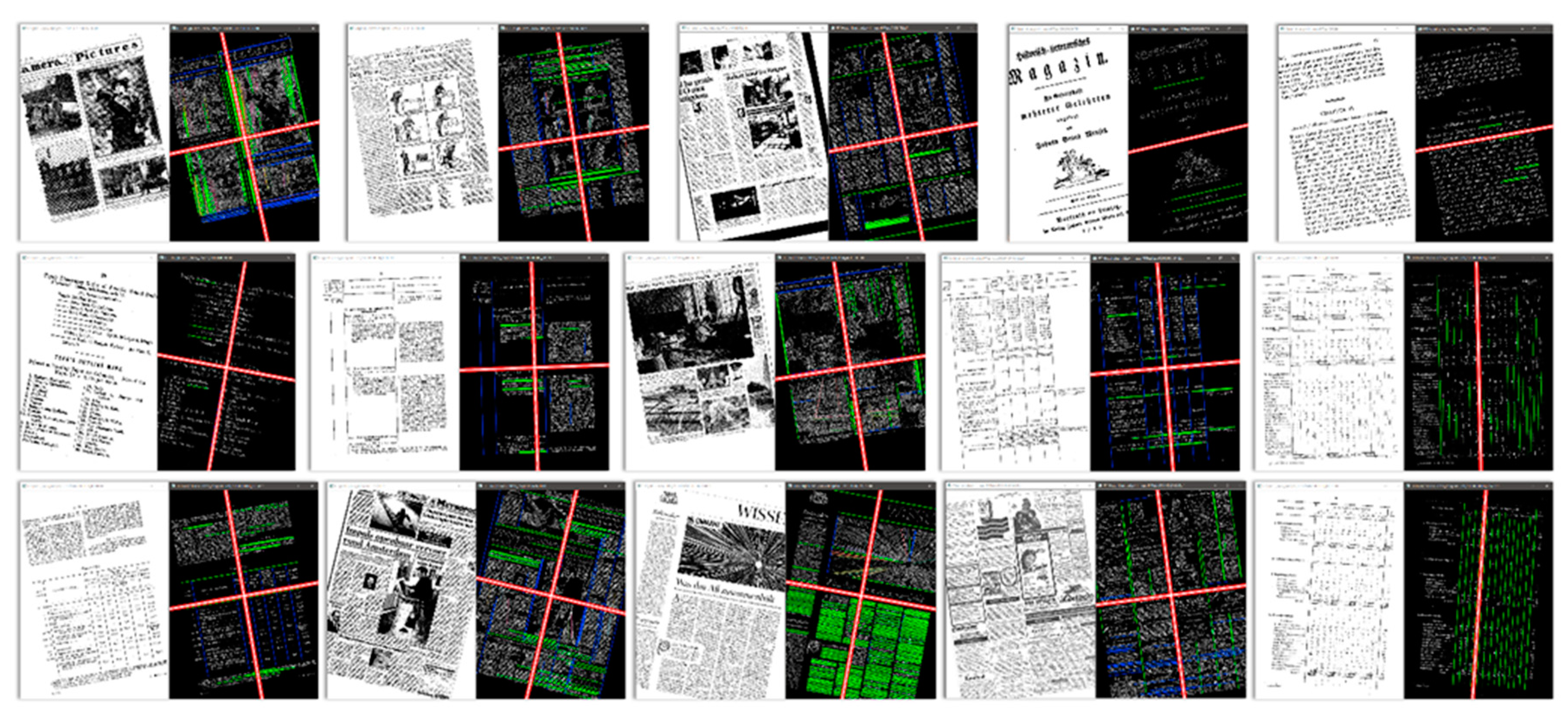
If there is more than one set, we sort the sets descending by the sum of their segments’ length and pick the first three or four sets (or two, if there are only two sets) as candidates for the horizontal and vertical axes of the document. If two of the sets have representatives that can be considered perpendicular, then the representatives will be picked as the document’s horizontal and vertical axes and the skew angle is computed as a weighted sum of the angles each representative makes with the closest primary axis. If there are no perpendicular representatives, then the first set in the sorted candidates is picked as the horizontal or vertical axis of the document, depending on the angle it makes with the primary axes.
In Figure 6, document orientation axes are shown passing through the center of processed images (black background), and for some images (e.g., the three rightmost images) only one axis was detected.
2.3.2. Confidence
The confidence for this algorithm, Equation (4), is computed as a product of one or multiple accuracy indicators, depending on which case we are in.
For any set of parallel lines, we can compute the average absolute dot-product , of the support vectors for all possible line pairs within the set. The closer this average is to one, the more parallel we can consider the lines, so the greater the algorithm’s confidence should be.
If we only have one set A, whose representative is pronounced as one of the document’s axes, then only the first factor ( is returned as the method’s confidence.
For two sets of segments, A and B, whose representatives and are pronounced as the document’s vertical and horizontal axes, then we can account on how close to perpendicular is to for computing confidence, by computing their dot product. The second factor in the confidence formula increases the measure when and tend to be perpendicular and decreases it when and tend to be parallel.
The third factor is responsible for a contribution equal to the ratio between the sum of lengths of all segments in A and B, which we write as and , respectively, and the sum of lengths of all segments in all sets, including A and B. This is performed in order to encourage the contribution of the longer segments in the final confidence formula because longer segments are both more reliably detected and their support angle is also more accurate.
Again, is a positive exponent used for fine-tuning the confidence to achieve balance and accuracy in the voting process.
3. Voting
In Section 2, we described three algorithms to compute the skew angle of a document and an expression for each algorithm to define a confidence level in the work it has done, as a number ranging between zero and one. In this section, we describe mechanisms that use the result and confidence of each algorithm to accurately determine the skew angle.
Besides the skew angle, is also offered in the end an aggregate confidence measure of the entire system. A user of a real-world document image processing application may use this measure to select only low-confidence (if any) image candidates and inspect them visually. The aggregate confidence is obtained as analogous to the skew angle for each of the following three voting methods and, as a result, it will not be further detailed.
3.1. Best First Voting
This method is the most basic, as it picks the result of the algorithm which returned the greatest confidence measure, completely discarding the others. It performs as expected, masking faults of algorithms in various situations, but not combining any results if confidences are close.
Another version of this policy is returning a weighted (by confidence) sum (or simply a mean) of the first two candidates, descending by confidence, while completely discarding the third.
3.2. Weighted Voting
This policy returns a weighted sum of the results returned by the algorithms, where the weights employed in the voting process are exactly the confidences returned by every skew detection method. This has the advantage of combining the results to increase the tolerance to errors. However, there must be a confidence threshold, below which a candidate is discarded. Otherwise, candidates with low confidence, i.e., an inaccurate result, would hijack the candidates who performed successfully. The low/high-confidence threshold is empirically set at 50%.
3.3. Unanimous Voting
All candidates are associated with equal weights for the voting process, except the low-confidence ones (those below a threshold empirically set at 50%), in which case their weight in the voting process becomes null, as described in Section 3.2.
4. Tests and Results
Our test dataset contains over 300 images representing both documents scanned by hand and digital documents converted into images. By introducing a random skew angle on each, we were able to correctly determine the accuracy of the system, knowing a priori what it should return.
In Table 1, we show a benchmark performed on our digital dataset with introduced skew. The test dataset contains a large diversity of document formats: from illustrated textbooks to scientific papers, poetry books, working sheets, art magazines, newspapers, CAD parts and more. It has been carefully selected such that there is diversity in structure, fonts, content (images/text) and abundance of orientation information. This dataset has been processed by applying random skew angles to each image and repeatedly fed to all three algorithms and the voting process while measuring accuracy and performance for each step. The results shown in Table 1 contain the following:
- execution time on a 64-bit Windows 7 system, i7-8550U CPU, using CPU-only OpenCV 4.01 routines, Microsoft Visual Studio 2017, with full compiler optimization for speed;
- average error, computed as the average absolute value of the difference between the known introduced skew angle and the skew angle detected by our system, for success cases, i.e., if the confidence is greater than some threshold (empirically chosen 50%);
- average confidence, taking into account both success and failure cases;
- uptime: the ratio between the number of success cases and the number of total cases.
For fine-tuning the exponent parameters of each algorithm’s confidence, we used the brute force search method, that is: for every triplet of exponents , discrete interval, we compute the average error for the entire dataset for every voting process. We picked φ = 0.8 and the step between elements in the interval ε = 0.025.
The brute-force search results in the space are presented in Table 2. Anyway, the system is not extremely sensitive regarding values, delivering robust results for most combinations as long as .
The Section Supplementary Materials contains a reference to the source code and the benchmarking dataset for this project.
5. Conclusions
The algorithms backed up for each other in failure cases, resulting in almost 100% uptime. The failure cases were, in fact, splash pages containing images, with almost no visual orientation information, such as lines aligned with the document’s primary axes.
The Best First voting method turned out to give the best results.
The average uptime for this voting policy is 99.5%, as only two images, which arguably do not contain any orientation information, were not deskewed correctly—both images contain organic paintings.
Having many algorithms attempting to solve the same problem, each performing on a different aspect of the problem, while being able to estimate a confidence measure of their work, is an optimal case for running all algorithms and returning a result determined by vote, which is closer to the ground truth than any of the candidate algorithms.
By fine-tuning the confidences of the candidate algorithms, we obtained a better uptime and overall accuracy.
The technology presented in this paper was developed and employed in the “Lib2Life- Revitalizing Libraries and Cultural Heritage through Advanced Technologies” project [31] aimed at both researching document image techniques suitable for automatic content creation and building of a large repository consisting from millions of pages of books, newspapers and journals with diverse content and spread across multiple time periods. Due to the large variations and unpredictability in the processing input, a strong need for algorithms that do not require user supervision emerged.
The voting-based deskew method was validated on a very demanding dataset, encompassing all kinds of complex layouts, tables, alignments and illustrations. Moreover, it was successfully used until now in the first part of the document image processing in the aforementioned project, on a little more than half a million pages and the results were visually examined by dense sampling. Very encouragingly, no erroneous rotations of the pages were reported, thus one can easily conclude that the proposed approach is indeed a very robust one, ideally suited for the mass production of digital content.
Supplementary Materials
The source code and the benchmarking dataset for this project may be found at the following link: https://gitlab.com/adix64/document-deskewer.
Author Contributions
Conceptualization, C.-A.B.; Data curation, O.-A.D.; Formal analysis, O.-A.D., C.P. (Cornel Popescu), N.C. and C.P. (Catalin Petrescu); Funding acquisition, C.-A.B., C.P. (Cornel Popescu), N.C. and C.P. (Catalin Petrescu); Methodology, C.-A.B.; Project administration, O.-A.D.; Resources, C.P. (Cornel Popescu), N.C. and C.P. (Catalin Petrescu); Software, O.-A.D.; Supervision, C.-A.B.; Validation, C.-A.B.; Visualization, C.-A.B. and O.-A.D.; Writing—original draft, C.-A.B.; Writing—review & editing, C.-A.B., O.-A.D., C.P. (Cornel Popescu), N.C. and C.P. (Catalin Petrescu). All authors have read and agreed to the published version of the manuscript.
Funding
This work was supported by a grant of the Romanian Ministry of Research and Innovation, CCCDI—UEFISCDI, project number PN-III-P1-1.2-PCCDI-2017-0689/„Lib2Life- Revitalizarea bibliotecilor si a patrimoniului cultural prin tehnologii avansate”/„Revitalizing Libraries and Cultural Heritage through Advanced Technologies”, within PNCDI III.
Conflicts of Interest
The authors declare no conflict of interest.
References
- Hull, J.J. Document image skew detection: Survey and annotated Bibliography. In Document Analysis Systems II; Hull, J.J., Taylor, S.S., Eds.; World Scientific: Singapore, 1998; pp. 40–64. [Google Scholar]
- Barekat Rezaei, S.; Sarrafzadeh, A.; Shanbezadeh, J. Skew Detection of Scanned Document Images. Lect. Notes Eng. Comput. Sci. 2013, 2202, 451–456. [Google Scholar]
- AL-Khatatneh, A.; Ali Pitchay, S.; Al-Qudah, M. A Review of Skew Detection Techniques for Documents. In Proceedings of the 17th UKSIM-AMSS International Conference on Modelling and Simulation, Cambridge, UK, 25–27 March 2015; pp. 316–321. [Google Scholar]
- Beusekom, J.; Shafait, F.; Breuel, T. Resolution Independent Skew and Orientation Detection for document images. Proc. SPIE Int. Soc. Opt. Eng. 2009, 7247, 1–10. [Google Scholar] [CrossRef] [Green Version]
- Lu, S.; Tan, C.L. Automatic document orientation detection and categorization through document vectorization. In Proceedings of the 14th Annual ACM International Conference on Multimedia, Santa Barbara, CA, USA, 23–27 October 2006; pp. 113–116. [Google Scholar] [CrossRef] [Green Version]
- Kanai, J.; Bagdanov, A.D. Projection profile based skew estimation algorithm for JBIG compressed images. Int. J. Doc. Anal. Recognit. (IJDAR) 1998, 1, 43–51. [Google Scholar]
- Hashizume, A.; Yeh, P.S.; Rosenfeld, A. A method for detecting the orientation of aligned components. Pattern Recognit. Lett. 1986, 4, 125–132. [Google Scholar] [CrossRef]
- Jiang, X.; Bunke, H.; Widmer-Kljajo, D. Skew detection of document images by focused nearest-neighbor clustering. In Proceedings of the Fifth International Conference on Document Analysis and Recognition (ICDAR-99), Bangalore, India, 20–22 September 1999; pp. 629–632. [Google Scholar]
- Zhang, Y.; Zhong, J.; Yu, H.; Kong, L. Research on Deskew Algorithm of Scanned Image. In Proceedings of the IEEE International Conference on Mechatronics and Automation (ICMA), Changchun, China, 5–8 August 2018; pp. 397–402. [Google Scholar]
- Shukla, B.K.; Kumar, G.; Kumar, A. An approach for Skew Detection using Hough Transform. Int. J. Comput. Appl. 2016, 136, 20–23. [Google Scholar]
- Ma, H.; Yu, Z. An enhanced skew angle estimation technique for binary document images. In Proceedings of the Fifth International Conference on Document Analysis and Recognition (ICDAR), IEEE, Bangalore, India, 20–22 September 1999; pp. 165–168. [Google Scholar]
- Mandip, K.; Simpel, J. An Integrated Skew Detection and Correction Using Fast Fourier Transform and DCT. Int. J. Sci. Technol. Res. 2013, 2, 164–169. [Google Scholar]
- Steinherz, T.; Intrator, N.; Rivlin, E. Skew detection via principal component analysis. In Proceedings of the Fifth International Conference on Document Analysis and Recognition (ICDAR-99), Bangalore, India, 20–22 September 1999; pp. 153–159. [Google Scholar]
- Aithal, P.K.; Rajesh, G.; Siddalingaswamy, P.C.; Acharya, D.U. A novel skew estimation approach using Radon transform. In Proceedings of the 11th International Conference on Hybrid. Intelligent Systems (HIS), Melacca, Malaysia, 5–8 December 2011; pp. 1–4. [Google Scholar]
- Papandreou, A.; Gatos, B. A Novel Skew Detection Technique Based on Vertical Projections. In Proceedings of the International Conference on Document Analysis and Recognition (ICDAR-2011), Beijing, China, 18–21 September 2011; pp. 384–388. [Google Scholar]
- Das, A.; Chanda, B. A fast algorithm for skew detection of document images using morphology. Int. J. Doc. Anal. Recognit. (IJDAR) 2001, 4, 109–114. [Google Scholar] [CrossRef]
- Geng, L.; Meng, Q.; Xiao, Z.; Liu, Y. Measurement of Period Length and Skew Angle Patterns of Textile Cutting Pieces Based on Faster R-CNN. Appl. Sci. 2019, 9, 3026. [Google Scholar] [CrossRef] [Green Version]
- Parhami, B. Voting algorithms. IEEE Trans. Reliab. 1995, 43, 617–629. [Google Scholar] [CrossRef] [Green Version]
- Wu, Z.; Fu, W.; Xue, R.; Wang, W. A Novel Line Space Voting Method for Vanishing-Point Detection of General Road Images. Sensors 2016, 16, 948. [Google Scholar] [CrossRef] [PubMed]
- Boiangiu, C.A.; Ioanitescu, R.; Dragomir, R.C. Voting-Based OCR System. Proc. J. ISOM (J. Inf. Syst. Oper. Manag.) 2016, 10, 470–486. [Google Scholar]
- Beaudoin, N.; Beauchemin, S. An Accurate Discrete Fourier Transform for Image Processing. In Object Recognition Supported by User Interaction for Service Robots, Proceedings of the 16th International Conference on Pattern Recognition (ICPR), Quebec, Canada, 11–15 August 2002; Institute of Electrical and Electronics Engineers: Piscataway, NJ, USA; Volume 3, pp. 935–939.
- Gupta, M.R.; Jacobson, N.P.; Garcia, E.K. OCR binarization and image pre-processing for searching historical documents. Pattern Recognit. 2007, 40, 389–397. [Google Scholar] [CrossRef]
- Hassanein, A.S.; Mohammad, S.; Sameer, M.; Ragab, M.E. A survey on Hough transform, theory, techniques and applications. Int. J. Comput. Sci. Issues (IJCSI) 2015, arXiv:1502.02160 [cs.CV]. [Google Scholar]
- Anuar, K.; Jambek, A.; Sulaiman, N. A study of image processing using morphological opening and closing processes. Int. J. Control Theory Appl. 2016, 9, 15–21. [Google Scholar]
- Varade, R.R.; Dhotre, M.R.; Pahurkar, A.B. A Survey on Various Median Filtering Techniques for Removal of Impulse Noise from Digital Images. Int. J. Adv. Res. Comput. Eng. Technol. (IJARCET) 2013, 2. Available online: http://ijarcet.org/wp-content/uploads/IJARCET-VOL-2-ISSUE-2-606-609.pdf (accessed on 10 March 2020).
- Rosner, D.; Boiangiu, C.A.; Zaharescu, M.; Bucur, I. Image Skew Detection: A Comprehensive Study. In Proceedings of the IWoCPS-3, The Third International Workshop On Cyber Physical Systems, Bucharest, Romania, 29–30 May 2014. Position 10. [Google Scholar]
- Cai, P.; Chandrasekaran, I.; Cai, Y.; Zheng, J.; Gong, I.; Lim, T.S.; Wong, P. Collision detection using axis aligned bounding boxes. In Simulations, Serious Games and Their Applications, Gaming Media and Social Effects; Cai, Y., Goei, S.L., Eds.; Springer Science+Business Media: Singapore, 2014; pp. 1–14. [Google Scholar]
- Liu, H.; Pang, L.; Li, F.; Guo, Z. Hough Transform and Clustering for a 3-D Building Reconstruction with Tomographic SAR Point Clouds. Sensors 2019, 19, 5378. [Google Scholar] [CrossRef] [PubMed] [Green Version]
- Kanopoulos, N.; Vasanthavada, N.; Baker, R.L. Design of an image edge detection filter using the Sobel operator. IEEE J. Solid-State Circuits 1988, 23, 358–367. [Google Scholar] [CrossRef]
- CCS’s DocWorks/Seamless Conversion/One Workflow. Zero Worries. Available online: https://content-conversion.com/wp-content/uploads/2020/02/CCS_docWorks_Folder.pdf (accessed on 10 March 2020).
- eLibraryBuilder—Lib2Life. Project Component of “Lib2Life- Revitalizing Libraries and Cultural Heritage through Advanced Technologies”, Grant PN-III-P1-1.2-PCCDI-2017-0689/PNCDI III. Available online: http://lib2life.ro/elibrary-builder/ (accessed on 10 March 2020).
Figure 1.
(a) Stripes image sample I; (b) Fast Fourier Transform (FFT)(I); (c) OTSU(FFT(I)).

Figure 2.
From left to right, top to down: Input, FFT of Input, Otsu on FFT of Input, processed FFT (with contrast stretching and histogram equalization), Otsu on the processed FFT, skew angle detection performed on the latter, using the Hough transform.
Figure 2.
From left to right, top to down: Input, FFT of Input, Otsu on FFT of Input, processed FFT (with contrast stretching and histogram equalization), Otsu on the processed FFT, skew angle detection performed on the latter, using the Hough transform.

Figure 3.
Two examples of frequency domain projection profiling, deskewing by variance maximization for each axis, i.e., finding the angle Θdeskew = argmaxΘ(σ2(H|(Θ)) + σ2(H─(Θ)).
Figure 3.
Two examples of frequency domain projection profiling, deskewing by variance maximization for each axis, i.e., finding the angle Θdeskew = argmaxΘ(σ2(H|(Θ)) + σ2(H─(Θ)).

Figure 4.
(a) Input: skewed document; (b) points of connected components’ axis-aligned bounding boxes (AABBs): top (blue) and bottom (red) sides and their associated scanline histograms; (c) same as ‘(b)’, but the histograms have maximum variance as the page is correctly oriented.
Figure 4.
(a) Input: skewed document; (b) points of connected components’ axis-aligned bounding boxes (AABBs): top (blue) and bottom (red) sides and their associated scanline histograms; (c) same as ‘(b)’, but the histograms have maximum variance as the page is correctly oriented.

Figure 5.
Projection profiling of AABBs’ edge midpoints, on the histogram.

Figure 6.
Document orientation detection using the detected lines in the spatial domain (black background), the algorithm performed on various documents (white background).
Figure 6.
Document orientation detection using the detected lines in the spatial domain (black background), the algorithm performed on various documents (white background).


Table 1.
Test results for the proposed skew detection system.
| Skew Detection Method | Execution Time | Average Error | Average Confidence | Uptime |
|---|---|---|---|---|
| Frequency Domain (FFT-based)* | 1451ms | 0.218° | 77% | 95% |
| Projection Profiling Row Align* | 1640ms | 0.553° | 77% | 94% |
| Spatial Domain Lines (Hough-based)* | 794ms | 0.128° | 82 % | 86% |
| PCA-based** | 2224ms | 0.396° | N/A | N/A |
| Radon Transform** | 800ms | 0.290° | N/A | N/A |
| Nearest-Neighbor Clustering** | 1822ms | 0.484° | N/A | N/A |
| Vertical Projections** | 3343ms | 0.272° | N/A | N/A |
| Morphology-based** | 2020ms | 0.402° | N/A | N/A |
| Best First Voting* | 3908ms | 0.111° | 94% | 99% |
| Weighted Voting* | 3908ms | 0.266° | 89% | 99% |
| Unanimous Voting* | 3908ms | 0.372° | 75% | 99% |
Notes: a) The execution times marked with * were obtained using the article’s demonstrator application. b) The execution times (and the subsequent deskewed images) marked with ** were obtained using the CCS’s DocWorks 6.8 commercial solution for creating digital libraries [30]. As a result, they should be used only qualitatively. Also, since the confidence measures are not defined in this case and they were also considered when measuring the uptime, in these cases no uptime can be provided for comparison.
Table 2.
Brute-force fine-tuning exponent search results.
| Voting Method | Frequency Domain (τ1) | Projection Profiling Row Align (τ2) | Spatial Domain Lines (τ3) |
|---|---|---|---|
| Best First | 0.25 | 1.05 | 1.21 |
| Weighted | 0.26 | 1.02 | 1.17 |
| Unanimous | 0.28 | 0.98 | 1.09 |
© 2020 by the authors. Licensee MDPI, Basel, Switzerland. This article is an open access article distributed under the terms and conditions of the Creative Commons Attribution (CC BY) license (http://creativecommons.org/licenses/by/4.0/).
Share and Cite
MDPI and ACS Style
Boiangiu, C.-A.; Dinu, O.-A.; Popescu, C.; Constantin, N.; Petrescu, C. Voting-Based Document Image Skew Detection. Appl. Sci. 2020, 10, 2236. https://doi.org/10.3390/app10072236
AMA Style
Boiangiu C-A, Dinu O-A, Popescu C, Constantin N, Petrescu C. Voting-Based Document Image Skew Detection. Applied Sciences. 2020; 10(7):2236. https://doi.org/10.3390/app10072236
Chicago/Turabian StyleBoiangiu, Costin-Anton, Ovidiu-Alexandru Dinu, Cornel Popescu, Nicolae Constantin, and Cătălin Petrescu. 2020. "Voting-Based Document Image Skew Detection" Applied Sciences 10, no. 7: 2236. https://doi.org/10.3390/app10072236
Note that from the first issue of 2016, this journal uses article numbers instead of page numbers. See further details here.