An Experimental Tuning Approach of Fractional Order Controllers in the Frequency Domain

Abstract

Fractional calculus has been used intensely in recent years in control engineering to extend the capabilities of the classical proportional–integral–derivative (PID) controller, but most tuning techniques are based on the model of the process. The paper presents an experimental tuning procedure for fractional-order proportional integral–proportional derivative (PI/PD) and PID-type controllers that eliminates the need of a mathematical model for the process. The tuning procedure consists in recreating the Bode magnitude plot using experimental tests and imposing the desired shape of the closed loop system magnitude. The proposed method is validated in the field of active vibration suppression by using an experimental set-up consisting of a smart beam.

1. Introduction

When subjected to the task of improving the performance of a physical process, classical control theory tackles the issue using two steps: mathematically modeling the dynamics of the process and tuning a suitable controller for the identified model.

Several alternatives have been developed for controller tuning based on information gained from the experimental response of the process. For most processes, transient and steady-state analysis of the process offers enough information to obtain a decent controller. However, there is no guarantee that the obtained controller is the ideal one. Experimental methods such as the well-known Ziegler Nichols, Kappa–Tau method, Cohen–Coon, Tyreus–Luyben, Ciancone, and Marlin tune classical proportional–integral–derivative (PID) controllers based on measurements of the different dynamics of the process response [1,2,3,4,5]. In most cases, the controllers tuned using experimental procedures lead to a closed loop system with poor robustness performance [6]. Robust autotuning has been proposed by [7] where the phase and magnitude margins are specified. The problem of autotuning robustness is also tackled in [8] by imposing the iso-damping property of the closed loop.

An increasing trend in controller design integrates the concept of fractional calculus. A rational order for the differentiation and integration extends the classical PID controller to a fractional-order PID. This type of controllers offer increased degrees of freedom and an increased stability as the number of tuned parameters increases [9,10]. One of the popular methods for tuning fractional-order controllers is by imposing frequency domain constraints such as the gain crossover frequency, phase margin, sensitivity, and complementary sensitivity [11]. Other frequency domain tuning procedures may also impose a flat phase around the gain crossover frequency guaranteeing a certain degree of robustness to gain variations [12,13]. Optimization techniques have also been used to successfully tune fractional-order controllers in the frequency domain [14,15]. Over the years, fractional calculus proved useful in both identification and control applications. Its numerous advantages have been successfully tested and validated on a manifold of real-life processes such as flexible transmission [16], active suspension [17], buck converters [18], hydraulic actuators [19], irrigation canals [20], pneumatic pressure [21], industrial distributed systems [22], robotic manipulators [23], etc.

The autotuning approach has also been applied in the fractional calculus controller design [24,25,26,27]. A fractional-order experimental tuning procedure based on a single experiment has been explored in [28]. The authors present the tuning of a fractional-order PD controller without using an identified model for the process [29]. The process is fed by a sinusoidal input and the amplitude and phase shifts of the output signal are measured. The output signal is then fed to a filter in order to determine the derivative of the signal. From the obtained information regarding the output amplitude, phase and the derivative slope, a fractional-order PD controller is determined. The Ziegler–Nichols method has been extended in order to tune a fractional-order PI controller in [30]. A fractional-order PID controller is tuned using a relay that takes the system at its stability margin in [31]. For the output signal, the amplitude and phase are measured and using the derivative of the phase the fractional-order PID controller is determined.

The presented work consists of joining the advantages of optimal controller tuning and experimental procedures. An optimal controller tuning in the frequency domain consists of determining the controller parameters such as the shape of the closed loop satisfies several constraints. A fractional-order controller is more suitable for the task, as in the frequency domain, the first-order integration/differentiation introduces a fixed slope of +20/−20 dB/decade and a fixed phase of +90/−90 degrees. A fractional-order integration/differentiation offers the flexibility of variable magnitude slope and a variable phase value. Therefore, a fractional controller is more suitable to honor closed loop frequency domain constraints. The tuning of the fractional-order controller is based on an optimization routine that considers the frequency response magnitude values obtained experimentally.

The main application to the developed method is vibration mitigation. This specific field has gained more popularity in recent years, especially in combination with fractional-order control. The complexity of control tasks associated to vibration suppression systems requires the usage of controllers based on more advanced mathematical tools, such as the fractional calculus branch. Many fractional-order controller tuning methodologies have been developed and tested with the sole purpose of vibration suppression. A fusion between a fractional-order disturbance observer and PI fuzzy controller is proposed in [32] to reduce vibration amplitude in an industrial servo system. Vibrations of an aeroplane wing modeled as a smart beam are suppressed using fractional-order PID-type controllers in [12,13,33,34,35]. Structural vibrations of uncertain systems are mitigated using a fractional-order sliding mode controller in [36]. Residual vibrations are tackled in [37] using adaptive-predictive fractional-order control strategies, whereas [38] uses optimal fractional-order controllers for AC motor vibrations.

The previously mentioned works use complex fractional-order tuning strategies, based on available models of vibration process’ dynamics. The control development is difficult and requires an advanced fractional-order background of the control engineer. In contrast, the experimental fractional-order tuning method presented throughout this study does not require any fractional order background, making the method ideal in industrial applications. From an engineer’s point of view, the presented fractional-order controller tuning procedure consists of two steps: The first one implies performing several experiments on the vibration platform, reading the vibration amplitude and experimental approximation of the resonant peak. The second step requires the choice of new magnitude values such as to ensure that the magnitude plot around the magnitude peak is flattened. The ease of application as well as the guaranteed vibration suppression results make the method ideal for industrial scenarios.

The novelty of the presented study is asserted in determining optimal fractional-order controller parameters based solely on the experimental response of the process. The method overcomes drawbacks encountered in classical auto-tuning practices by imposing the magnitude and phase of the closed loop system. A certain degree of robustness can also be assured is the phase margin constraints are imposed to satisfy the iso-damping property. The proposed strategy is appropriate to tune fractional-order proportional derivative (PD), proportional integral (PI), and PID controllers with similar tuning effort.

The developed methodology is validated experimentally on a vibration unit consisting of a smart beam. The movement of the beam is controlled using piezoelectric actuators placed near the fixed end, whereas the displacement is measured with a strain gauge sensor. The choice of the experimental platform lies in its versatility: the smart beam can be correlated to physical systems such as aeroplane wings, helicopter rotors, cantilever beams, suspended platforms, blades of various heavy-duty machinery, etc.

The paper presents the mathematical background of the proposed tuning procedure in Section 2. The method is viable to tune fractional-order PI-, PD-, and PID-type of controllers. Section 3 presents the experimental platform consisting of a smart beam used to prove the efficacy of the proposed method. A fractional-order PD controller is tuned in Section 4, whereas a fractional-order PID is tuned in Section 5. The obtained controllers are validated by analyzing disturbance rejection capabilities.

2. Proposed Tuning Method

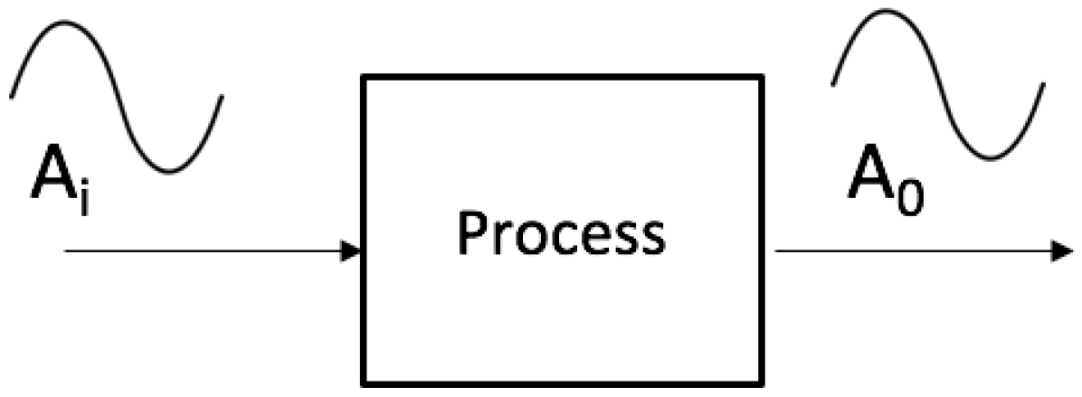
The proposed tuning procedure is based on experimental tests without the need of a model for the process. By excluding the model, one can also remove modeling errors and uncertainties, and it also eliminates the need of using a fractional-order model or a high order model in the case of more complex processes. The method has its basis in the Bode magnitude plot which can be created experimentally by feeding the process a series of sine wave signals of a given amplitude $A_i$ and a given frequency $\omega$. As can be seen in Figure 1, for a sinusoidal input, the output of the process will be a sinusoidal output of the same given frequency $\omega$, but with a different amplitude $A_o$ and a phase shift $\tau$.

Performing several sine wave tests recreates part of the magnitude frequency diagram through points. The method resides solely on measuring the amplitudes of the input and output signals and computing the corresponding frequency response magnitude values and does not include measurements regarding the time shift, facilitating its ease in real-life applications. The minimum number of points needed resides in the type of the desired controller. Every chosen point of the Bode diagram is part of a system of equations that needs to be solved in order to find the controller parameters, therefore the minimum number of tests needed is equal to the number of controller parameters.

After performing the experimental tests and determining several magnitude values at their corresponding frequencies, the process Bode magnitude plot can be recreated. Next, the shape of the closed loop can be imposed by analyzing the actual values of the open loop magnitude. Taking as an example the vibration phenomenon, which exhibits a resonant characteristic, the magnitude at the resonant frequency should be close to 0, as well as the magnitude at the frequencies near the resonance. In real-life situations, this results in a diminished amplitude of oscillation with less visible effects.

Starting from the following values of the process’ magnitude, obtained via the experimental sine tests as described above, for n different frequencies:

$$\left\{\begin{array}{c}|G\left({\omega }_1\right)|=mag{G}_{1}dB,\hfill \\ |G\left({\omega }_2\right)|=mag{G}_{2}dB,\hfill \\ \dots \hfill \\ |G\left({\omega }_n\right)|=mag{G}_{n}dB.\hfill \end{array}\right.$$

(1)

The desired magnitude and phase of the closed loop at the chosen frequencies are chosen such as

$$\left\{\begin{array}{c}|H_0\left({\omega }_1\right)|=mag{H}_{1}dB,\angle \left(H_0\left({\omega }_1\right)\right)=phaseH1deg,\hfill \\ |H_0\left({\omega }_2\right)|=mag{H}_{2}dB,\angle \left(H_0\left({\omega }_2\right)\right)=phaseH2deg,\hfill \\ \dots \hfill \\ |H_0\left({\omega }_n\right)|=mag{H}_{n}dB,\angle \left(H_0\left({\omega }_n\right)\right)=phaseHndeg.\hfill \end{array}\right.$$

(2)

Choosing the closed loop design specifications at specific frequencies results in shaping the closed loop magnitude and phase diagrams. The main focus of the specifications is to guarantee the disturbance rejection around the resonant frequency by imposing the magnitude value at the resonant frequency close to 0dB. The other magnitude values are chosen such that the slope of the magnitude graph is smoother than the uncompensated system implying an increased damping. The phase constraints are chosen such that the close loop system is stable and a certain degree of robustness is obtained through the iso-damping property.

The closed loop transfer function written depending on the process and the controller for a negative feedback system can be written as

$$H_0\left(s\right)=\frac{G\left(s\right)C\left(s\right)}{1+G\left(s\right)C\left(s\right)},$$

(3)

from which the open loop can be deduced as being

$$G\left(s\right)C\left(s\right)=\frac{H_0\left(s\right)}{1-H_0\left(s\right)}.$$

(4)

Mapping the Laplace domain to the frequency domain by replacing $s=j\omega$, the frequency domain open loop equation becomes

$$G\left(j\omega \right)C\left(j\omega \right)=\frac{H_0\left(j\omega \right)}{1-H_0\left(j\omega \right)}.$$

(5)

Expressing the magnitude of the closed loop in dB is done by

$${\left|G\left(j\omega \right)C\left(j\omega \right)\right|}^{dB}=20{log}_{10}\frac{|H_0\left(j\omega \right)|}{|1-H_{0.}\left(j\omega \right)|}.$$

(6)

The magnitude of the controller in dB is written as

$${\left|C\left(j\omega \right)\right|}^{dB}={\left|G\left(j\omega \right)C\left(j\omega \right)\right|}^{dB}-{\left|G\left(j\omega \right)\right|}^{dB}.$$

(7)

The magnitude of the open loop, denoted by $\left|G\right(j\omega \left)C\right(j\omega \left)\right|$, can be determined from Equation (5) if the magnitude of $1-H_0\left(j\omega \right)$ is determined. In order to do so, the closed loop is written as a sum of its real and imaginary parts, denoted by $A\left(\omega \right)$ and $B\left(\omega \right)$, respectively.

$$H_0\left(j\omega \right)=A\left(\omega \right)+jB\left(\omega \right).$$

(8)

The real and imaginary parts give the magnitude of the open loop

$$|H_0\left(j\omega \right)|=\sqrt{A{\left(\omega \right)}^2+B{\left(\omega \right)}^2}$$

(9)

and the phase

$$\angle H_0\left(j\omega \right)=arctan\frac{B\left(\omega \right)}{A\left(\omega \right)}.$$

(10)

Equation (2) imposes values for the closed loop magnitude and phase such that some design specifications are met. Equations (9) and (10) form a system of two equations with two unknowns, $A\left(\omega \right)$ and $B\left(\omega \right)$. By solving the system created, the values of the real and imaginary parts are obtained. Replacing the magnitudes of $|1-H_0\left(j\omega \right)|$ with the values of $A\left(\omega \right)$ and $B\left(\omega \right)$ allows the computation of the values for ${\left|G\left(j\omega \right)C\left(j\omega \right)\right|}^{dB}$ based on Equation (6) and further allows for the estimation of the values of the magnitude of the controller from Equation (7).

Repeating the steps for n test frequencies leads to a system of n equations where the known variable is the magnitude of the controller and the unknowns are the controller parameters.

$$\left\{\begin{array}{c}|C\left({\omega }_1\right)|=mag{C}_{1}dB,\hfill \\ |C\left({\omega }_2\right)|=mag{C}_{2}dB,\hfill \\ \dots \hfill \\ |C\left({\omega }_n\right)|=mag{C}_{n}dB.\hfill \end{array}\right.$$

(11)

Customizing the system of equations for the desired type of controller and solving the system should lead to the controller parameters. The system should be solved using numerical optimization routines, such that the best combination of parameters is found. It is highly recommended to take into consideration the following.

• The minimum number of equations needed, denoted by n, depends on the complexity of the chosen controller. The minimum n should be greater or equal than the number of parameters that need to be tuned.
• A constrained routine can be chosen to perform the optimization such that one of the equations from the system is minimized, while the other equations are regarded as constraints.
• As in any optimization algorithm, the developed solution depends on the chosen starting point and the initial points should be chosen realistically. For example, in the case of a fractional-order differentiation, the derivative order belongs to the interval $(0,1]$.

The proposed tuning method is suitable for tuning classical PID type controllers as well as their fractional-order extensions. A generalization of the PI/PD controller is characterized by the following equation,

$$C_{FO-PI/PD}=k_p+k_d{s}^{\mu },$$

(12)

where $k_p$ and $k_i$ are the proportional and derivative gains, whereas $\mu$ gives the type of the controller,

• $\mu =-1$ integer order PI controller
• $\mu =1$ integer order PD controller
• $\mu \in (-1,0)$ fractional-order PI controller
• $\mu \in (0,1)$ fractional-order PD controller

Choosing this type of controller for the process requires a minimum of three experimental frequency domain tests, as there are three parameters that need to be tuned. If the results obtained by the fractional-order PI/PD controller are not satisfactory, a more complex fractional-order PID may be required:

$$C_{FO-PID}=k_p+k_d{s}^{\mu }+\frac{k_i}{s^{\lambda }},$$

(13)

where $k_p$, $k_d$, and $k_i$ are the proportional, derivative, and integral gains, whereas $\mu \in (0,1]$ denotes the order of the differentiation and $\lambda \in [-1,0)$ expresses the order of the integration. The fractional PID requires a minimum number $n=5$ of experimental tests in order to develop the system needed for the controller optimization.

The focus of the method is mitigating vibration. The optimization approach is related to the frequency domain magnitude and phase. The method guarantees the computation of a viable fractional-order controller that efficiently suppresses vibration. It is important to emphasize that the efficiency of the obtained fractional-order controller lies in a stable, robust, closed-loop system that reduces the effect of the vibration on the process. The tuning methodology is focused on flattening the resonant peak that causes real-life vibration mitigation, without specific attention to the closed-loop system’s performance such as settling time.

As the method is an experimental one and does not require a mathematical model for the process, validating the method will be done on an experimental platform.

3. Experimental Platform

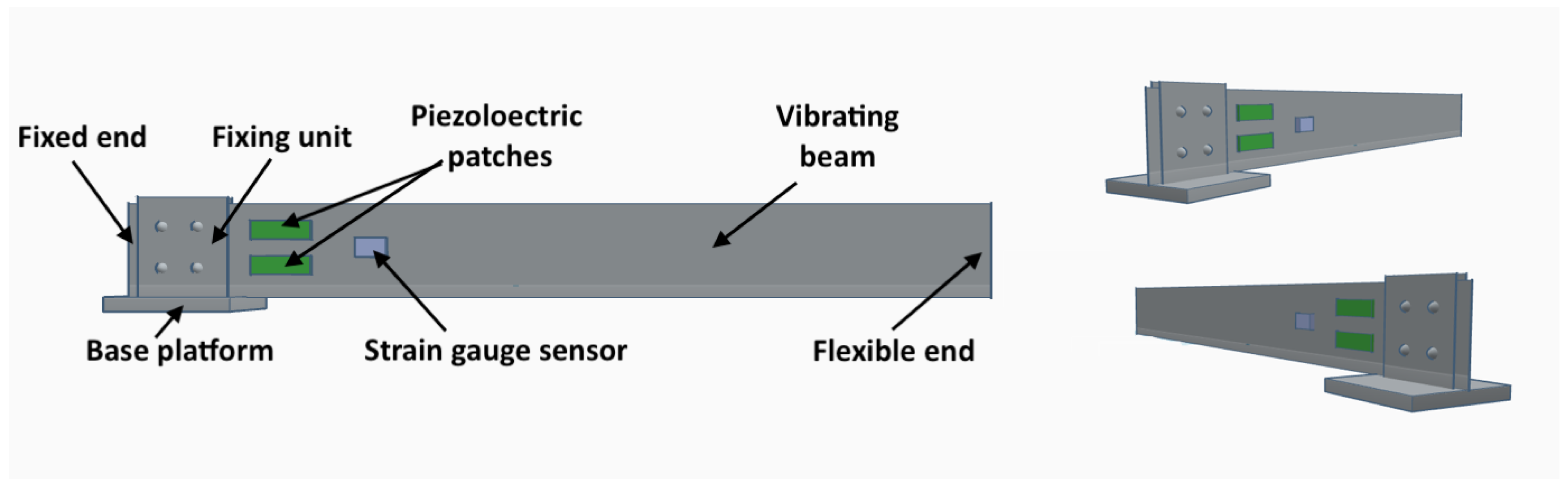
The experimental setup consists of a 250 mm long, 20 mm wide, and 1 mm thick aluminum beam whose vibration is being measured and controlled. The beam is equipped with 4 piezoelectric DuraAct P-878 Power Patch PZT patches, placed two on each side, near the fixed end. Figure 2 presents a 3D model of the set-up. The purpose of two patches from one side is to generate beam oscillations with a given frequency and amplitude, thus giving the possibility to generate a certain disturbance, whereas the other two are used for testing the developed controllers. The fractional controllers are evaluated based on disturbance rejection; the purpose of the controllers being to maintain the free end of the beam from vibrating.

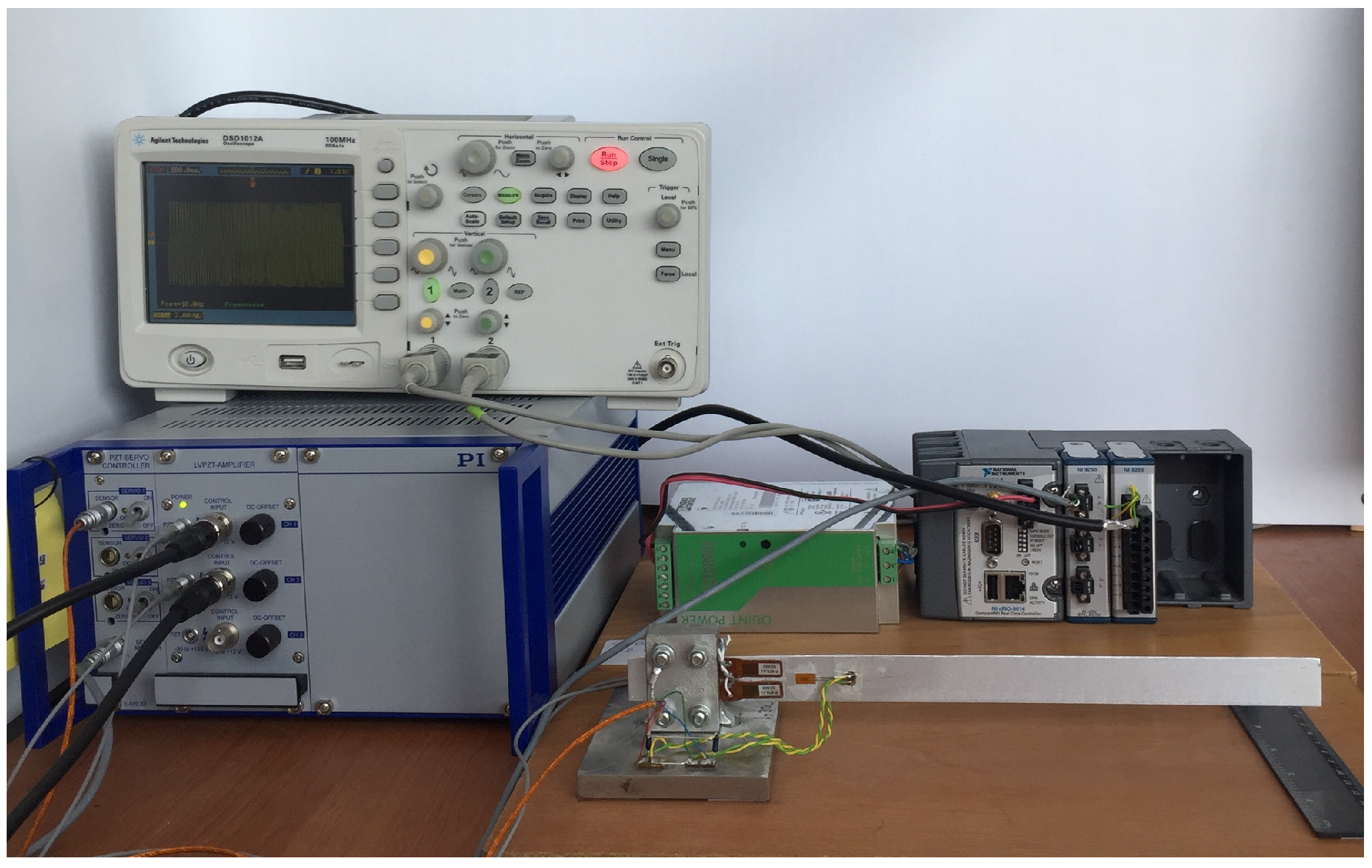
The control signal is computed in real-time using $LabVIE{W}^{\mathrm{TM}}$ and is sent to the beam using the CompactRIO${}^{\mathrm{TM}}$ 9014 controller. The NI 9263 output module excites the PZT patches on the beam, while the NI 9230 input module measures the displacement of the free end using the 120 ohm Omega Prewired KFG-5-120-C1-11L1M2R strain gauge sensors. An additional E-509.X3 module from Physik Instrumente amplifies the signal received from the strain gause sensors, while the E-503.00 amplifies the signal from the PZT patches. A block diagram of the set-up is presented in Figure 3.

The position of the patches on the beam and a more detailed view of the real workbench is provided in Figure 4.

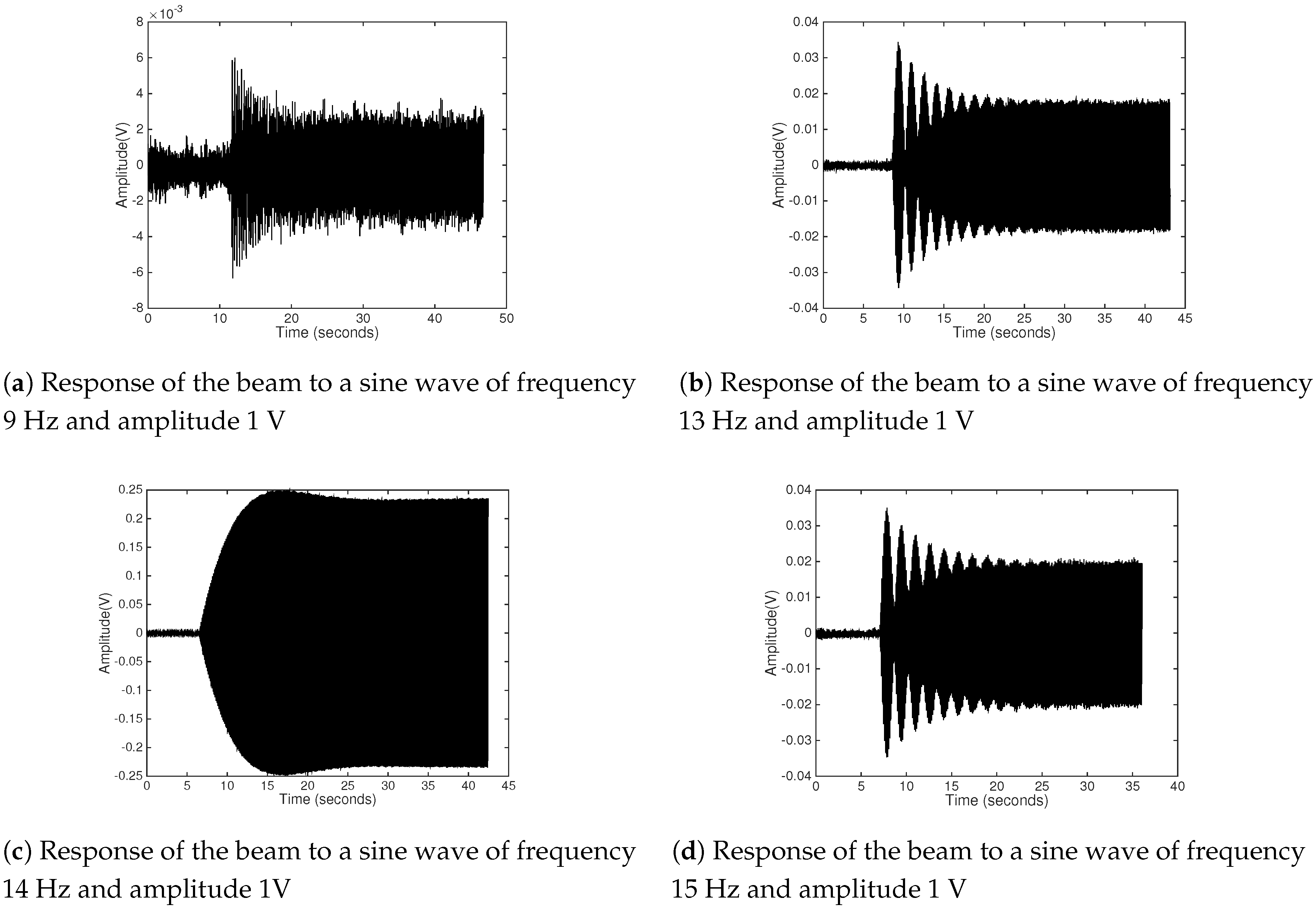
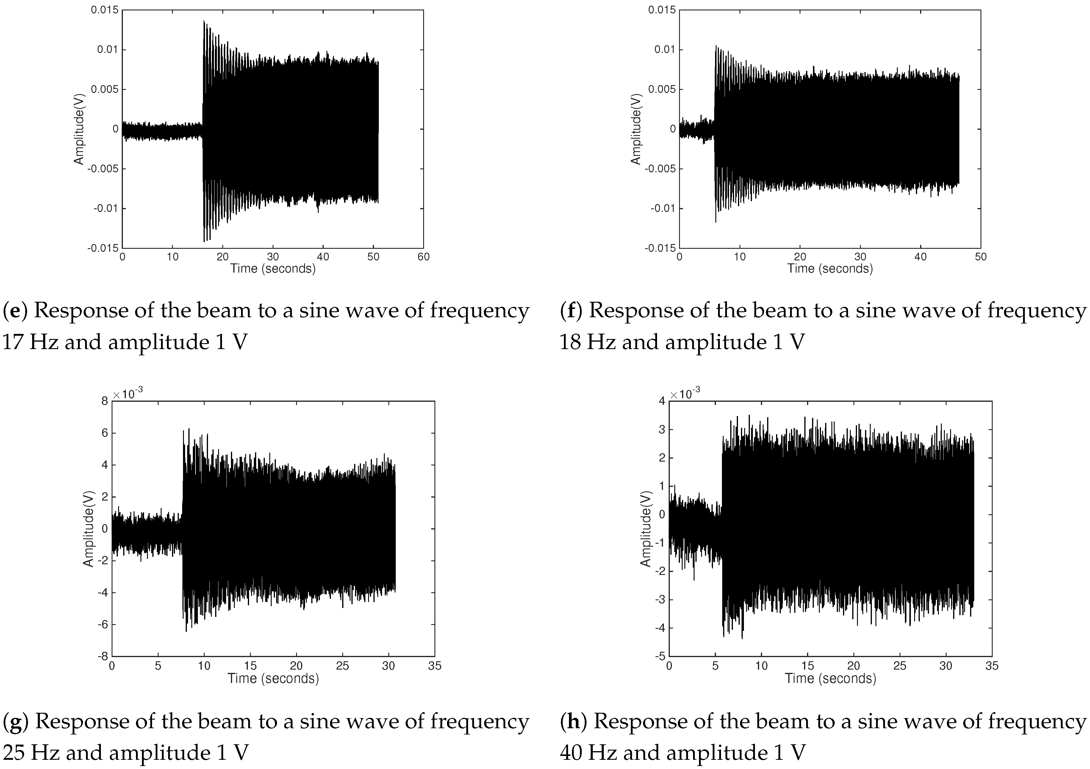
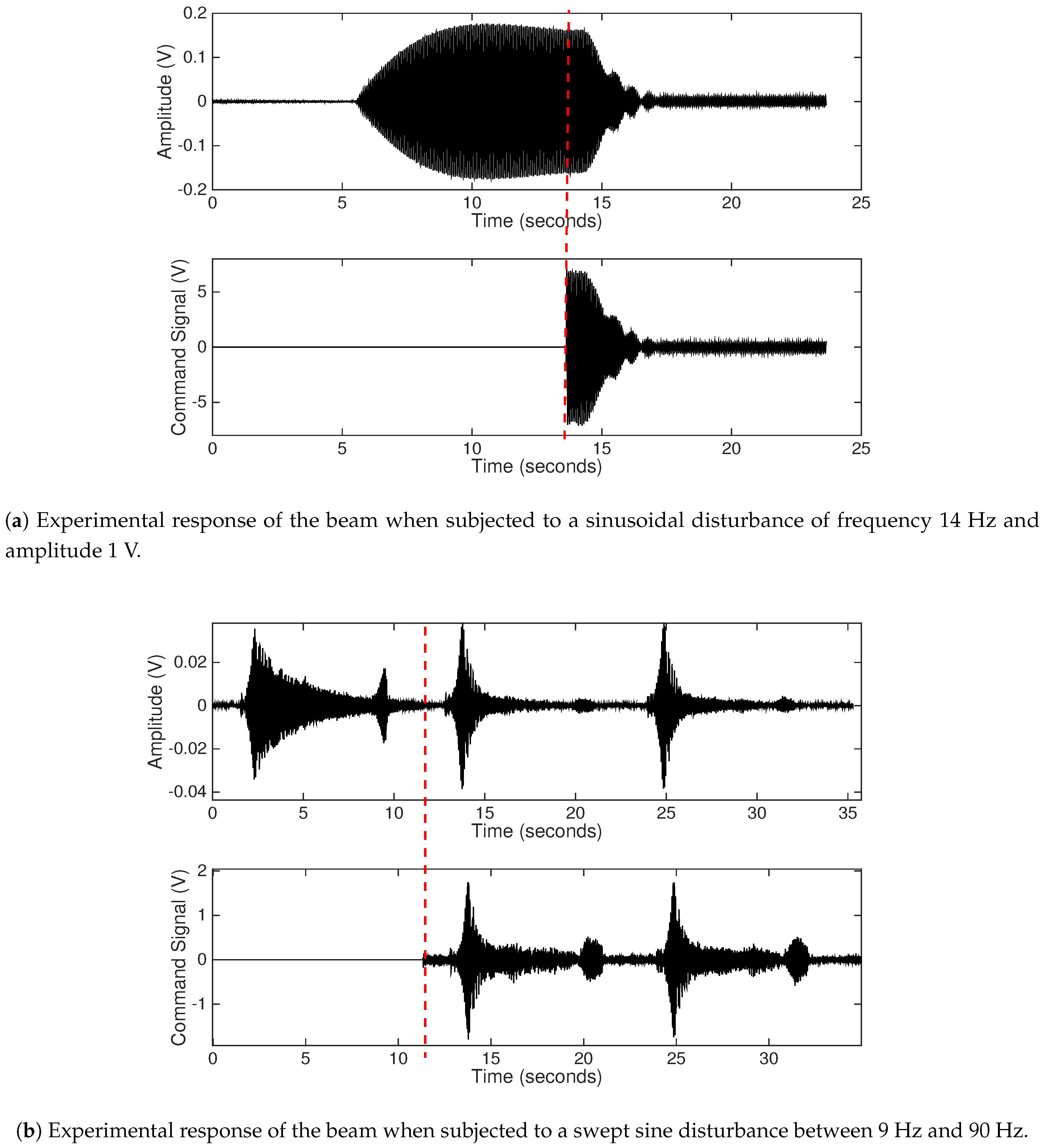
Several experimental tests were performed for different frequencies, and the response of the beam is presented in the figures below. The frequencies chosen are around the resonant frequency, as for this frequency the movement of the beam has the greatest amplitude. The first resonant frequency of the smart beam has been experimentally determined at 14 Hz, as can be seen in Figure 5c.

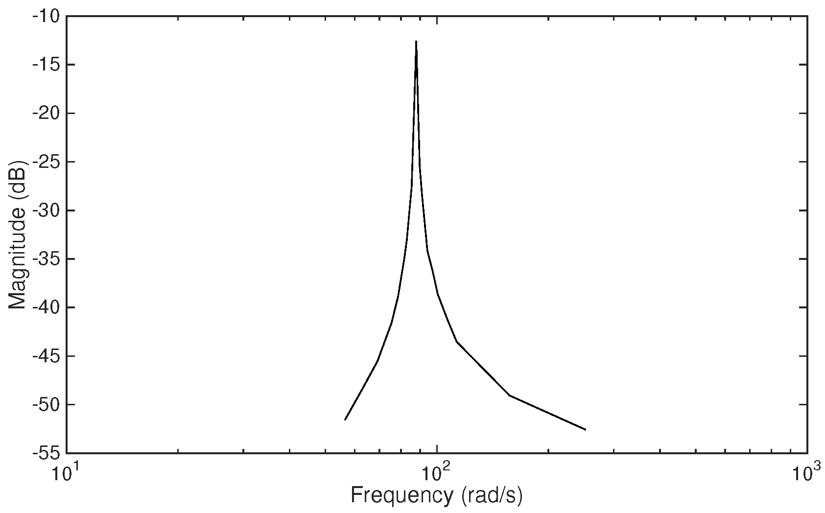
The Bode magnitude plot was created from data given in Figure 5. Taking as an example Figure 5c, where a sine wave of frequency 14 Hz is given as an input, the measured output amplitude is 0.2355 V. Transforming 14 Hz to rad/s with the formula $f_{rad/s}=f_{Hz}\ast 2\ast \pi$ gives 87.9645 rad/s, whereas 0.2355V to dB using $A_{dB}=20\ast {log}_{10}A$ gives −12.5602 dB, giving one point of the Bode diagram from Figure 6. Due to the physical limitations of the test, it is impossible to measure the amplitude for frequencies outside the measured domain because of the low ratio between the measured amplitude and noise sensitivity.

4. Controller Tuning

4.1. Optimization Guidelines

The tuning methodology presented in Section 2 is mainly focused on shaping the Bode magnitude plot. The controller tuning procedure is transformed into a system with multiple nonlinear equations composed of the magnitude of the system at various frequencies. The objective is to find an optimal shape of the magnitude plot that flattens the resonant peak of the system. The optimization can be realized in programs such as MATLAB using functions such as the fmincon function provided by the Optimization Toolbox. As in any optimization routine, the starting point for the parameters is paramount in obtaining a valid solution. The proper choice of the pivot point ensures that the provided solution avoids the local minima problem.

When dealing with a fractional-order PID controller, there are five parameters that need to be computed through the optimization procedure: A relevant starting point should be chosen such that the obtained controller is viable in a real life implementation. The fractional orders of differentiation and integration span in the $\left[01\right]$ interval. Therefore, any value inside the interval represents a correct choice for the initial condition in the optimization.

However, for the case of the proportional, integral, and derivative gains, the choice for the initial values is more difficult. Illustrating the basic principles on choosing relevant starting points, a fractional-order PD transfer function is considered:

$$H_c\left(s\right)=k_p\left(1+T_d{s}^{\mu }\right),$$

(14)

where $k_p$ is the proportional gain, $T_d$ is the derivative time constant, and $\mu$ is the fractional order of differentiation $\mu \in \left[01\right]$.

The effect of the fractional-order controller on the magnitude plot will be analyzed further. The magnitude of $H_c\left(s\right)$ can be written as $\left|H_c\left(j\omega \right)\right|=\left|k_p\right||1+T_d{\left(j\omega \right)}^{\mu }|$. The effects of the magnitude of $H_c\left(j\omega \right)$ will be analyzed further considering the individual contribution of $\left|k_p\right|$ and $|1+T_d{\left(j\omega \right)}^{\mu }|$.

In an open-loop system, $H_{ol}\left(j\omega \right)=H_p\left(j\omega \right)H_c\left(j\omega \right)$, the magnitude representation of $H_{ol}\left(j\omega \right)$ is realized through graphical addition between the magnitude of $H_p\left(j\omega \right)$ and $H_c\left(j\omega \right)$. The same applies for the individual terms of $H_c\left(j\omega \right)$. The proportional gain and derivative time constant are computed based on the assumption that the contribution of every term of the controller is maximum. Looking at the process magnitude plot in Figure 6, the resonant magnitude should be moved closed to 0 dB, according to the methodology presented in Section 2. Therefore, the controller should move the process’ magnitude upwards by approximately 15 dB. Assuming that the proportional gain causes the 15 dB movement, one may write that $\left|k_p\right|=15dB=5.62$. Therefore, any value close to 5.62 may be chosen as the optimization starting point of the proportional gain.

Furthermore, the starting point for the derivative time constant can be approximated using the assumption that $|1+T_d{\left(j\omega \right)}^{\mu }|$ introduces the 15dB magnitude shift. Using de Moivre’s formula, one may write $1+T_d{\left(j\omega \right)}^{\mu }=1+T_d{\omega }^{\mu }\left(cos\frac{\mu \pi }{2}+jsin\frac{\mu \pi }{2}\right)$. The magnitude of the derivative part can be written as

$$|1+T_d{\left(j\omega \right)}^{\mu }|=\sqrt{{\left(1+T_d{\omega }^{\mu }cos\frac{\mu \pi }{2}\right)}^2+{\left(T_d{\omega }^{\mu }sin\frac{\mu \pi }{2}\right)}^2}.$$

(15)

Opening the brackets and using the trigonometric property ${sin}^2\frac{\mu \pi }{2}+{cos}^2\frac{\mu \pi }{2}=1$ gives

$$|1+T_d{\left(j\omega \right)}^{\mu }|=\sqrt{1+2T_d{\omega }^{\mu }cos\frac{\mu \pi }{2}+T_d^2{\omega }^{2\mu }}=15dB.$$

(16)

Replacing $\omega$ = ${\omega }_r=14Hz=87.9rad/s$, based on Figure 6, leads to

$$|1+T_d{\left(j{\omega }_r\right)}^{\mu }|=\sqrt{1+2T_d{87.9}^{\mu }cos\frac{\mu \pi }{2}+T_d^2{87.9}^{2\mu }}=5.62.$$

(17)

Knowing that $\mu \in \left[01\right]$ and evaluating the solution of (17) for $\mu =0$ gives $T_{d1}=-175.37$ and $T_{d2}=0.1744$, whereas for $\mu =1$, $T_d=\pm 0.0629$. Note that $T_d$ should always be greater than 0. Therefore, the starting point of $T_d$ can be chosen any value around $\left[0.06290.1744\right]$.

The guidelines can be extended for the fractional-order PI or PID controller. Note that in the following subsections the PD controller transfer function is slightly different and the derivative gain $k_d=T_d{k}_p$ interval is $k_d\in \left[0.35350.9801\right]$.

4.2. Fractional Order PI/PD Tuning

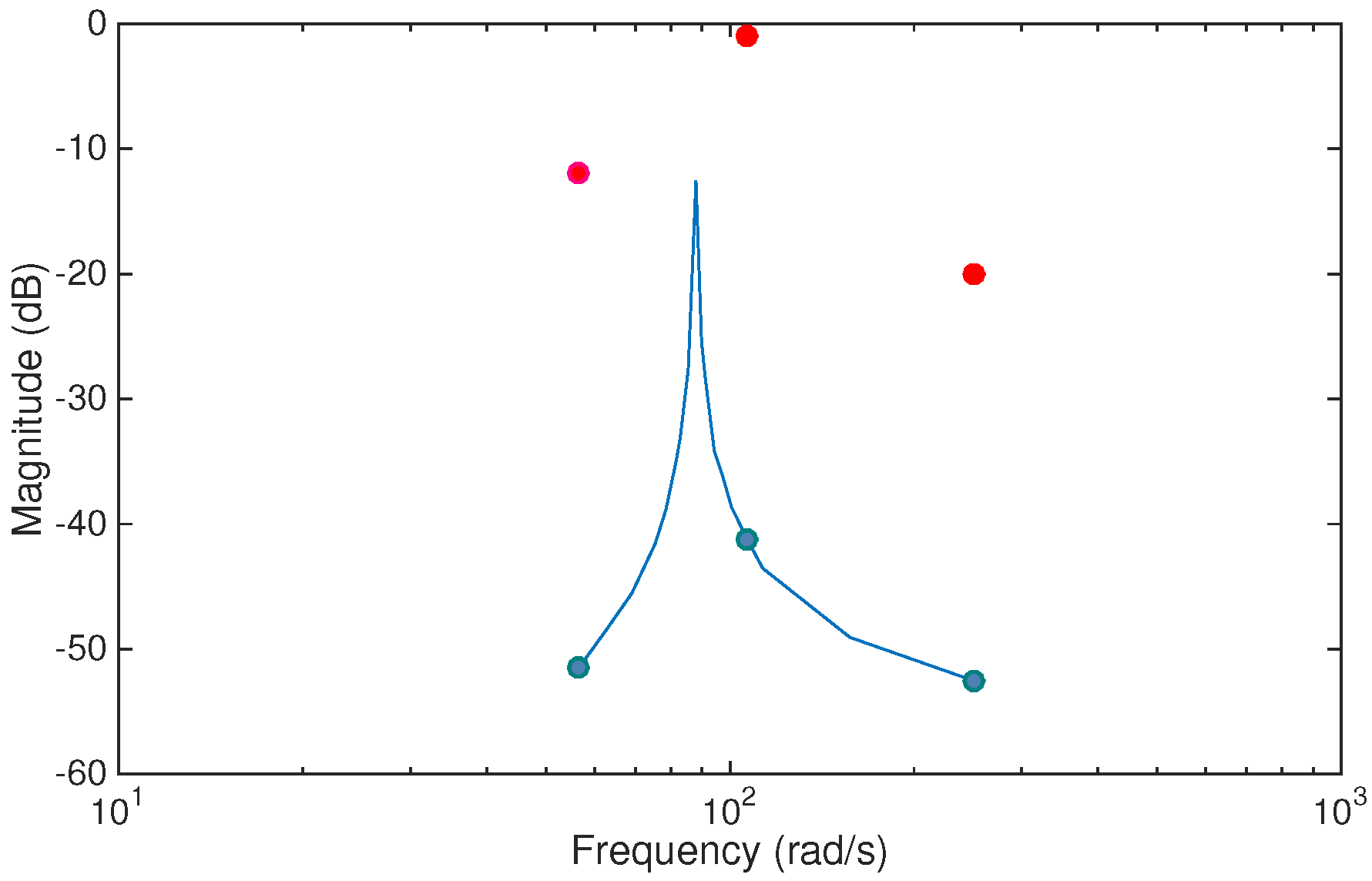
A fractional-order PD controller is first designed to suppress unwanted vibrations in the smart beam. As the controller’s transfer function has three parameters that have to be computed: $k_p$, $k_d$, and $\mu$, three points are computed on the magnitude diagram as follows,

$$\left\{\begin{array}{c}|G\left({\omega }_1\right)|=-51.52dB,{\omega }_1=56.55rad/s,\hfill \\ |G\left({\omega }_2\right)|=-41.25dB,{\omega }_2=107rad/s,\hfill \\ |G\left({\omega }_3\right)|=-52.55dB,{\omega }_3=251.3rad/s.\hfill \end{array}\right.$$

(18)

The three frequencies are chosen as follows; ${\omega }_2$ is close to the resonant frequency of the beam; and ${\omega }_1$ and ${\omega }_3$ are chosen to enclose the resonant frequency, and for the beam case they are chosen as the smallest/greatest frequency for which the magnitude of the process can be computed due to the physical limitations of the experimental set-up. The imposed magnitude and phase closed loop values for the chosen points are

$$\left\{\begin{array}{c}|H_0\left({\omega }_1\right)|=-12dB,\angle \left(H_0\left({\omega }_1\right)\right)=-0.1deg,\hfill \\ |H_0\left({\omega }_2\right)|=-1dB,\angle \left(H_0\left({\omega }_2\right)\right)=-60deg,\hfill \\ |H_0\left({\omega }_3\right)|=-20dB,\angle \left(H_0\left({\omega }_3\right)\right)=-120deg.\hfill \end{array}\right.$$

(19)

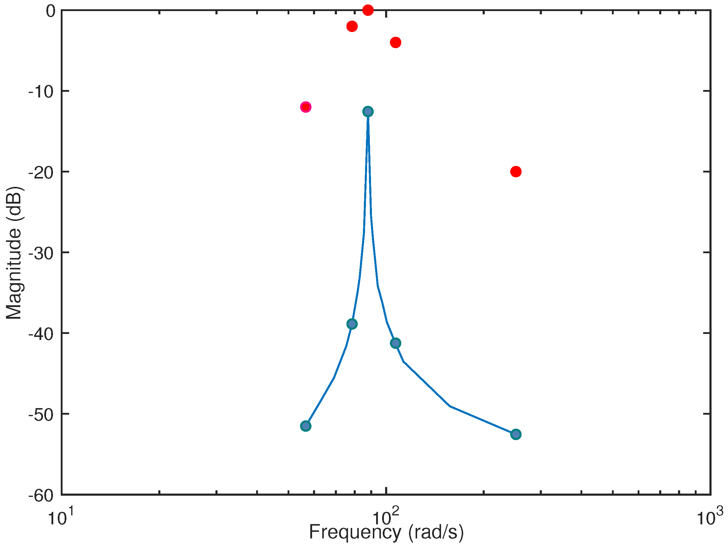
The constraints are imposed to ensure a lower resonant peak, larger damping, and a stable closed loop system. The graphical representation of the chosen constraints can be seen in Figure 7.

The optimization routine searches the solution of the minimization problem for $k_p\in \left(0100\right)$, $k_d\in \left(0100\right)$, and $\mu \in [-11]$. The initial points chosen for the parameters are $k_p=15$, $k_d=0.5$, and $\mu =0.85$. The controller determined that honors the imposed constraints for the closed loop magnitude and phase is a fractional-order PD controller:

$$C_{FO-PI/PD}=8+0.8888s^{0.7683}.$$

(20)

The obtained fractional-order PD controller is approximated to a 6th-order discrete transfer function using the method in [39], which is based on mapping the time Laplace operator directly into discrete time. The controller is validated in terms of disturbance rejection.

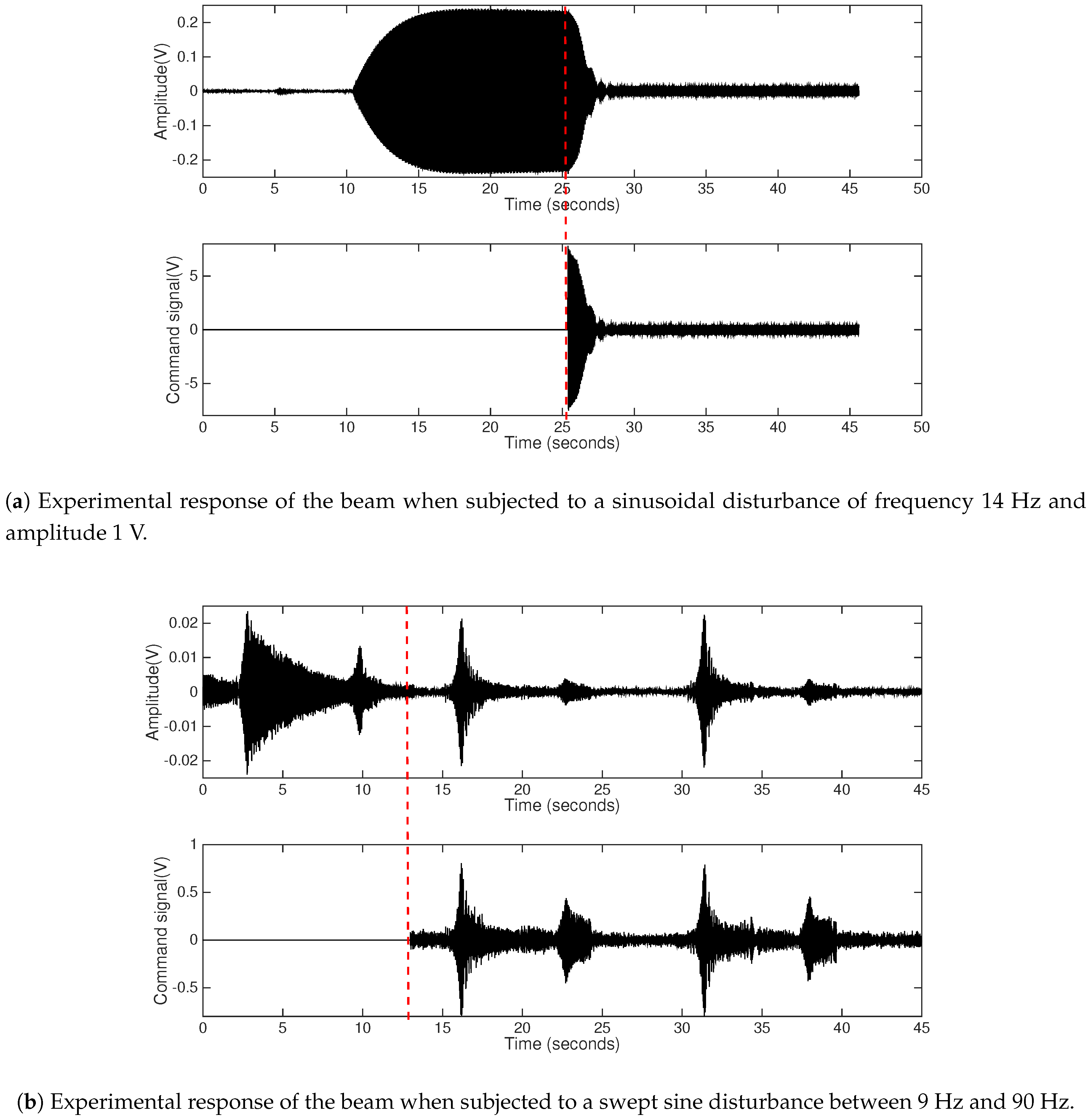
First, a sinusoidal input of the resonant frequency, 14 Hz, and an amplitude of 1V is given as a disturbance and the response of the beam is presented in Figure 8a. The uncompensated response of the beam leads to an amplitude of 0.25 V. The action of the controller is included at t = 25 s, and the fractional PD controller reduces the oscillation amplitude by 80% with a settling time of 2.5 s. The obtained controller is validated on a larger interval by giving a swept sine input with frequencies between 9 and 90Hz. Two resonant frequencies, representing the first and second flexural modes of the beam, can be visible at 14 Hz and 83 Hz. Figure 8b presents a test performed with the swept sine input for the uncompensated system and two more tests with the control action turned on. It can be seen that the amplitude of the beam is lowered for the entire frequency range.

4.3. Fractional-Order PID Tuning

In the previous section, the experimental method was successfully used to tune a fractional-order PD controller. The obtained controller proved useful in the case of disturbance rejection making the controller suitable for the chosen process. However, to prove the efficacy of the proposed method, a more complex fractional-order PID controller is tuned. The transfer function of the fractional PID from (13) has five parameters: $k_p$, $k_i$, $k_d$, $\lambda$, and $\mu$. Therefore, a minimum number of five points must be chosen from the magnitude plot.

$$\left\{\begin{array}{c}|G\left({\omega }_1\right)|=-51.52dB,{\omega }_1=56.55rad/s,\hfill \\ |G\left({\omega }_2\right)|=-38.87dB,{\omega }_2=78.54rad/s,\hfill \\ |G\left({\omega }_3\right)|=-12.56dB,{\omega }_3=87.96rad/s,\hfill \\ |G\left({\omega }_4\right)|=-41.25dB,{\omega }_4=107rad/s,\hfill \\ |G\left({\omega }_5\right)|=-52.55dB,{\omega }_5=251.3rad/s.\hfill \end{array}\right.$$

(21)

The frequencies from Equation (17) are chosen as follows; ${\omega }_3$ is the resonant frequency of the beam as can be seen in Figure 6; ${\omega }_1$ and ${\omega }_5$ are lower and upper bounds of the measured frequencies interval, respectively; and ${\omega }_2$ and ${\omega }_4$ are evenly distributed frequencies between the resonant peak frequency and the upper and lower bounds, respectively.

The closed loop magnitude and phase are imposed as

$$\left\{\begin{array}{c}|H_0\left({\omega }_1\right)|=-12dB,\angle \left(H_0\left({\omega }_1\right)\right)=-0.1deg,\hfill \\ |H_0\left({\omega }_2\right)|=-2dB,\angle \left(H_0\left({\omega }_2\right)\right)=-60deg,\hfill \\ |H_0\left({\omega }_3\right)|=-1dB,\angle \left(H_0\left({\omega }_3\right)\right)=-120deg,\hfill \\ |H_0\left({\omega }_4\right)|=-4dB,\angle \left(H_0\left({\omega }_4\right)\right)=-120deg,\hfill \\ |H_0\left({\omega }_5\right)|=-20dB,\angle \left(H_0\left({\omega }_5\right)\right)=-120deg.\hfill \end{array}\right.$$

(22)

Figure 9 presents the chosen values for the magnitude. The magnitude values are chosen in order to reduce the amplitude of the closed loop system at the resonant frequency, therefore ensuring a lower damping. The phase values are chosen such that the closed loop system is stable. The advantage of using a fractional-order PID controller over a fractional-order PD is that robustness can also be a design specification through the iso-damping property. The phase constraints are imposed to be $\angle H_0\left({\omega }_3\right)=\angle H_0\left({\omega }_4\right)=\angle H_0\left({\omega }_5\right)=-120deg$, resulting in a constant phase margin ${\varphi }_m=60deg$ between the frequencies belonging to the interval $[{\omega }_3,{\omega }_5]$, ensuring a certain robustness to small gain variations.

Initial points have been given for the optimization routine consisting of $k_p=15$, $k_d=0.05$, $k_i=0.05$, $\mu =0.85$ and $\lambda =0.15$. The obtained fractional-order PID controller by performing the minimization for $k_p\in (0,100)$, $k_d\in (0,100)$, $k_i\in (0,100)$, $\mu \in [0,1]$, and $\lambda \in [0,1]$ is given by

$$C_{FO-PID}=15.4506+0.8278s^{0.8220}+\frac{0.1}{s^{0.1049}}.$$

(23)

The obtained fractional-order PID controller has been approximated using the same complexity, 6^th order, and the same settling time, $T_s=0.005s$, as the fractional-order PD controller. Implementing the PID controller on the experimental unit successfully diminishes the effect of the disturbance, as can be seen in Figure 10a,b. For a sinusoidal disturbance of 14 Hz and 1V the oscillation amplitude is reduced by 80% and the settling time is around 3 s. The same tests are performed as in the case of the fractional-order PD controller, but the results are different because the two controllers were tuned with different closed loop magnitude and phase constraints. The purpose of tuning the PID controller is not to outperform the fractional PD, but to prove that the method is applicable to different controllers. The fractional-order PD and PID are different controllers tuned using the same method and validated on the same equipment, under the same conditions.

4.4. Robustness Analysis

Robustness to gain variations is indirectly imposed by the constraints for the phase in the interval comprising the resonant frequency. A straight line for the phase in an interval of frequencies ensure that, for small gain variations, the phase margin remains unchanged.

The tuning of the fractional-order PID controller ensures robustness by specifying closed loop phase values in order to honor the iso-damping property. The closed loop phase constraints from Equation (18) strive to achieve a flat phase between ${\omega }_3=87.96rad/s$ and ${\omega }_5=251.3rad/s$, attaining robustness to small gain variations.

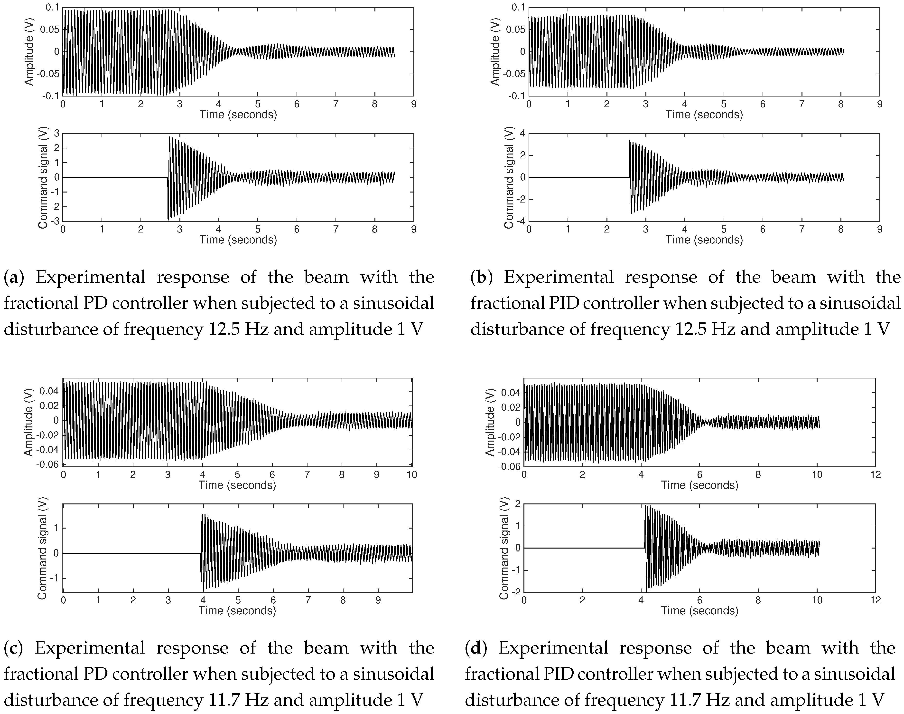
In order to experimentally test the robustness of the obtained controllers from Equations (16) and (19), weights have been added to the free end of the beam such that the resonant frequency is moved from 14 Hz to 12.5 Hz and 11.7 Hz, respectively. Two Neodymium–Iron–Boron permanent magnetic disks with 10mm diameter, 5 mm height, 30 g weight, and 1kg strength were placed on each side of the free end of the beam. The magnets were attached at a 3 cm distance to the moving end, centered with respect to the upper and lower margins of the beam. The tuned fractional-order PD and PID controllers were tested for sinusoidal disturbances of the new resonant frequency.

Figure 11a,b presents the data obtained using the fractional controllers when the resonant frequency of the beam is 12.5 Hz. For the fractional-order PD controller, the settling time is 1.5 s, whereas the PID attenuates and the vibration in approximately 1 s. The oscillation amplitude is reduced by 75% with the fractional-order PD and by 80% with the fractional-order PID controller.

Another test is performed when the resonant frequency of the beam is 11.7 Hz and the experimental data obtained with the two controllers is represented in Figure 11c,d. The settling time offered by the fractional-order PD is 2.5 s and the amplitude is reduced by 60%. The fractional-order PID controller reduces the amplitude by 78% in a settling time less than 2 s.

The fractional-order PID overall performance in terms of oscillation amplitude and settling time attenuation is better than the fractional-order PD performance, proving experimentally that the PID controller is more robust. The theoretical explanation is that in the case of the fractional-order PD controller, as there were three constraints imposed, only one constraint was imposed for the phase near the resonant frequency being impossible to impose a robustness condition. However, for the fractional-order PID, three equal phase margin constraints are imposed, leading to a closed loop flat phase around the resonant frequency making the controller robust.

5. Conclusions

The paper presents a tuning procedure for optimal fractional-order controllers based on the frequency domain response. The need of a process model is completely eliminated, making the method easily applicable to complex processes where a higher order model is needed. By eliminating the need of knowing the mathematical representation of the process’ dynamics, the tuning procedure eliminates modeling errors.

Most experimental methods are based on measuring both the amplitude and the time shift of the output signal. However, for the chosen process, the presented work has the major advantage of measuring only the output magnitude, completely excluding time shift measurements.

The chosen process for the method validation is a smart beam equipped with piezoelectric actuators. Two fractional-order controllers are tuned with the purpose of diminishing the effect of disturbances on the beam. A fractional-order PD controller and a more complex, fractional-order PID are determined through constrained optimization routines. The tuning process consists first in determining the process frequency response magnitude as some key frequencies based on experimental tests. Next, the closed loop frequency response magnitude and phase values are imposed at these key frequencies, according to some performance specifications. Using these closed loop frequency response magnitude and phase values, the constrained optimization routine is used to estimate the fractional-order controller parameters. The tuning effort is the same for any type of fractional-order controller chosen. The difference between tuning different controllers is the number of chosen points from the frequency diagram as optimization constraints.

The experimental results prove that the proposed method can be successfully used to tune fractional-order controllers in the absence of a process model.

References

- Aström, K.J.; Hägglund, T. PID Controllers: Theory, Design, and Tuning, 2nd ed.; Instrument Society of America: Research Triangle Park, NC, USA, 1995. [Google Scholar]
- de Souza, M.R.S.B.; Murofushi, R.H.; Tavares, J.P.Z.d.S.; Ribeiro, J. Comparison Among Experimental PID Auto Tuning Methods for a Self-balancing Robot. In Robotics: 12th Latin American Robotics Symposium and Third Brazilian Symposium on Robotics, LARS 2015/SBR 2015, Uberlândia, Brazil, 28 October–1 November 2015; Revised Selected Papers; Springer International Publishing: Cham, Switzerland, 2016; pp. 72–86. [Google Scholar] [CrossRef]
- Keyser, R.D.; Maxim, A.; Copot, C.; Ionescu, C.M. Validation of a multivariable relay-based PID autotuner with specified robustness. In Proceedings of the 2013 IEEE 18th Conference on Emerging Technologies Factory Automation (ETFA), Cagliari, Italy, 10–13 September 2013; pp. 1–6. [Google Scholar] [CrossRef] [Green Version]
- Nishikawa, Y.; Sannomiya, N.; Ohta, T.; Tanaka, H. A method for auto-tuning of PID control parameters. Automatica 1984, 20, 321–332. [Google Scholar] [CrossRef]
- Jahanshahi, E.; Sivalingam, S.; Schofield, J.B. Industrial test setup for autotuning of PID controllers in large-scale processes: Applied to Tennessee Eastman process. IFAC-PapersOnLine 2015, 48, 469–476. [Google Scholar] [CrossRef]
- Åström, K.; Hägglund, T. Revisiting the Ziegler–Nichols step response method for PID control. J. Process Control 2004, 14, 635–650. [Google Scholar] [CrossRef]
- Åström, K.J.; Hägglund, T. Automatic tuning of simple regulators with specifications on phase and amplitude margins. Automatica 1984, 20, 645–651. [Google Scholar] [CrossRef] [Green Version]
- Chen, Y.; Moore, K.L. Relay Feedback Tuning of Robust PID Controllers with Iso-damping Property. Trans. Syst. Man Cyber. Part B 2005, 35, 23–31. [Google Scholar] [CrossRef] [PubMed]
- Vilanova, R.; Visioli, A. PID Control in the Third Millennium: Lessons Learned and New Approaches; Springer: Berlin, Germany, 2012. [Google Scholar]
- Chen, Y.; Petras, I.; Xue, D. Fractional order control—A tutorial. In Proceedings of the 2009 American Control Conference, St. Louis, MO, USA, 10–12 June 2009; pp. 1397–1411. [Google Scholar] [CrossRef]
- Monje, C.A. Fractional-Order Systems and Controls: Fundamentals and Applications; Springer: London, UK, 2010. [Google Scholar]
- Muresan, C.I.; Birs, I.R.; Folea, S.; Dulf, E.H.; Prodan, O. Experimental results of a fractional order PDμ controller for vibration suppresion. In Proceedings of the 2016 14th International Conference on Control, Automation, Robotics and Vision (ICARCV), Phuket, Thailand, 13–15 November 2016; pp. 1–6. [Google Scholar] [CrossRef]
- Birs, I.R.; Folea, S.; Copot, D.; Prodan, O.; Muresan, C.I. Comparative analysis and experimental results of advanced control strategies for vibration suppression in aircraft wings. In Proceedings of the 2016 13th European Workshop on advanced Control and Diagnosis, Lille, France, 17–18 November 2016. [Google Scholar]
- Birs, I.R.; Muresan, C.I.; Folea, S.; Prodan, O.; Kovacs, L. Vibration suppression with fractional-order PIλDμ controller. In Proceedings of the 2016 IEEE International Conference on Automation, Quality and Testing, Robotics (AQTR), Cluj-Napoca, Romania, 19–21 May 2016; pp. 1–6. [Google Scholar] [CrossRef] [Green Version]
- Birs, I.R.; Folea, S.; Muresan, C.I. An optimal fractional-order controller for vibration attenuation. In Proceedings of the 2017 25th Mediterranean Conference on Control and Automation (MED), Valletta, Malta, 3–6 July 2017; pp. 828–832. [Google Scholar] [CrossRef]
- Oustaloup, A.; Mathieu, B.; Lanusse, P. The CRONE Control of Resonant Plants: Application to a Flexible Transmission. Eur. J. Control 1995, 1, 113–121. [Google Scholar] [CrossRef]
- Tseng, H.E.; Hrovat, D. State of the art survey: Active and semi-active suspension control. Veh. Syst. Dyn. 2015, 53, 1034–1062. [Google Scholar] [CrossRef]
- Calderón, A.J.; Vinagre, B.M.; Feliu, V. Fractional order control strategies for power electronic buck converters. Signal Process. 2006, 86, 2803–2819. [Google Scholar] [CrossRef]
- Maddahi, A.; Sepehri, N.; Kinsner, W. Fractional-Order Control of Hydraulically Powered Actuators: Controller Design and Experimental Validation. IEEE/ASME Trans. Mechatron. 2019, 24, 796–807. [Google Scholar] [CrossRef]
- Feliu-Batlle, V.; Rivas-Perez, R.; Castillo-Garcia, F.J.; Sanchez-Rodriguez, L.; Linarez-Saez, A. Robust fractional-order controller for irrigation main canal pools with time-varying dynamical parameters. Comput. Electron. Agric. 2011, 76, 205–217. [Google Scholar] [CrossRef]
- Al-Dhaifallah, M.; Kanagaraj, N.; Nisar, K.S. Fuzzy Fractional-Order PID Controller for Fractional Model of Pneumatic Pressure System. Math. Probl. Eng. 2018, 2018. [Google Scholar] [CrossRef] [Green Version]
- Abdelbaky, M.; El-Hawwary, M.; Emara, H. Implementation of fractional-order PID controller in an industrial distributed control system. In Proceedings of the 2017 14th International Multi-Conference on Systems, Signals & Devices (SSD), Marrakech, Morocco, 28–31 March 2017; pp. 713–718. [Google Scholar] [CrossRef]
- Sharma, R.; Rana, K.P.; Kumar, V. Performance analysis of fractional order fuzzy PID controllers applied to a robotic manipulator. Expert Syst. Appl. 2014, 41, 4274–4289. [Google Scholar] [CrossRef]
- Monje, C.A.; Vinagre, B.M.; Feliu, V.; Chen, Y. On auto-tuning of fractional order PIλDμ controllers. IFAC Proc. Vol. 2006, 39, 34–39. [Google Scholar] [CrossRef]
- Monje, C.; Vinagre, B.; Calderón, A.; Feliu, V.; Chen, Y. Auto-tuning of fractional lead-lag compensators. IFAC Proc. Vol. 2005, 38, 319–324. [Google Scholar] [CrossRef]
- Alagoz, B.B.; Ates, A.; Yeroglu, C. Auto-tuning of PID controller according to fractional-order reference model approximation for DC rotor control. Mechatronics 2013, 23, 789–797. [Google Scholar] [CrossRef]
- Jin, C.Y.; Ryu, K.H.; Sung, S.W.; Lee, J.; Lee, I.B. PID auto-tuning using new model reduction method and explicit PID tuning rule for a fractional order plus time delay model. J. Process Control 2014, 24, 113–128. [Google Scholar] [CrossRef]
- Muresan, C.; Keyser, R.D.; Birs, I.; Folea, S.; Prodan, O. An Autotuning Method for a Fractional Order PD Controller for Vibration Suppression. In Proceedings of the 2017 International Workshop Mathematical Methods in Engineering (MME 2017), Ankara, Turkey, 27–29 April 2017. [Google Scholar]
- Keyser, R.D.; Muresan, C.I.; Ionescu, C.M. A novel auto-tuning method for fractional order PI/PD controllers. ISA Trans. 2016, 62, 268–275. [Google Scholar] [CrossRef]
- Gude, J.J.; Kahoraho, E. Modified Ziegler-Nichols method for fractional PI controllers. In Proceedings of the 2010 IEEE 15th Conference on Emerging Technologies Factory Automation (ETFA 2010), Bilbao, Spain, 13–16 September 2010; pp. 1–5. [Google Scholar] [CrossRef]
- Monje, C.A.; Vinagre, B.M.; Feliu, V.; Chen, Y. Tuning and auto-tuning of fractional-order controllers for industry applications. Control Eng. Pract. 2008, 16, 798–812. [Google Scholar] [CrossRef] [Green Version]
- Li, W.; Hori, Y. Vibration suppression using single neuron-based PI fuzzy controller and fractional-order disturbance observer. IEEE Trans. Ind. Electron. 2007, 54, 117–126. [Google Scholar] [CrossRef]
- Onat, C.; Şahin, M.; Yaman, Y. Fractional controller design for suppressing smart beam vibrations. Aircr. Eng. Aerosp. Technol. 2012. [Google Scholar] [CrossRef]
- Muresan, C.I.; Folea, S.; Birs, I.R.; Ionescu, C. A novel fractional-order model and controller for vibration suppression in flexible smart beam. Nonlinear Dyn. 2018, 93, 525–541. [Google Scholar] [CrossRef]
- Birs, I.R.; Muresan, C.I.; Folea, S.; Prodan, O. A Comparison between Integer and Fractional Order PDμ Controllers for Vibration Suppression. Appl. Math. Nonlinear Sci. 2016, 1, 273–282. [Google Scholar] [CrossRef] [Green Version]
- Aghababa, M.P. A fractional-order controller for vibration suppression of uncertain structures. ISA Trans. 2013, 52, 881–887. [Google Scholar] [CrossRef] [PubMed]
- Lu, J.; Xie, W.; Zhou, H.; Zhang, A. Vibration suppression using fractional-order disturbance observer based adaptive grey predictive controller. J. Vibroeng. 2014, 16, 2205–2215. [Google Scholar]
- Zhao, H.; Deng, W.; Yang, X.; Li, X.; Dong, C. An optimized fractional order PID controller for suppressing vibration of AC motor. J. Vibroeng. 2016, 18, 2205–2220. [Google Scholar] [CrossRef]
- De Keyser, R.; Muresan, C.I.; Ionescu, C.M. An efficient algorithm for low-order direct discrete-time implementation of fractional order transfer functions. ISA Trans. 2018, 74, 229–238. [Google Scholar] [CrossRef] [PubMed]
Figure 1.
Sinusoidal input and output.
Figure 2.
3D model of the experimental set-up.
Figure 3.
Block diagram of the experimental set-up.
Figure 4.
Snapshot of the experimental set-up.
Figure 5.
Experimental response of the beam to sinusoidal inputs of different frequencies.
Figure 6.
Experimental Bode magnitude plot.
Figure 7.
Frequency domain magnitude constraints for fractional-order proportional integral–proportional derivative (PI/PD) tuning (blue—computed magnitude of the open loop system; red—imposed magnitude for the closed loop system).
Figure 8.
Experimental disturbance rejection of the closed loop system with the fractional-order PD controller.
Figure 9.
Frequency domain magnitude constraints for fractional-order proportional–integral– derivative (PID) tuning (blue—experimental magnitude values; red—imposed magnitude values for the closed loop system).
Figure 10.
Experimental disturbance rejection of the closed loop system with the fractional-order PID controller.
Figure 11.
Experimental robustness validation when altering the resonant frequency of the beam.
© 2020 by the authors. Licensee MDPI, Basel, Switzerland. This article is an open access article distributed under the terms and conditions of the Creative Commons Attribution (CC BY) license (http://creativecommons.org/licenses/by/4.0/).
Share and Cite
MDPI and ACS Style
Birs, I.; Folea, S.; Prodan, O.; Dulf, E.; Muresan, C. An Experimental Tuning Approach of Fractional Order Controllers in the Frequency Domain. Appl. Sci. 2020, 10, 2379. https://doi.org/10.3390/app10072379
AMA Style
Birs I, Folea S, Prodan O, Dulf E, Muresan C. An Experimental Tuning Approach of Fractional Order Controllers in the Frequency Domain. Applied Sciences. 2020; 10(7):2379. https://doi.org/10.3390/app10072379
Chicago/Turabian StyleBirs, Isabela, Silviu Folea, Ovidiu Prodan, Eva Dulf, and Cristina Muresan. 2020. "An Experimental Tuning Approach of Fractional Order Controllers in the Frequency Domain" Applied Sciences 10, no. 7: 2379. https://doi.org/10.3390/app10072379
Note that from the first issue of 2016, this journal uses article numbers instead of page numbers. See further details here.