Feature Selection for Facial Emotion Recognition Using Cosine Similarity-Based Harmony Search Algorithm

 ,
,  ,
,  , and
, and
Abstract
:1. Introduction
2. Motivation and Related Work
3. Dataset and Feature Description
3.1. Dataset Description
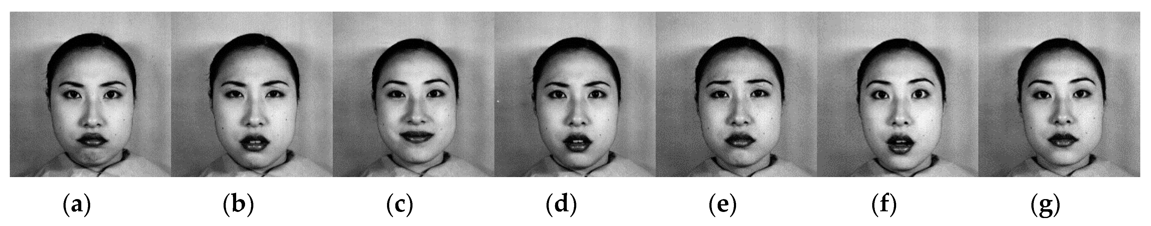
3.1.1. JAFFE
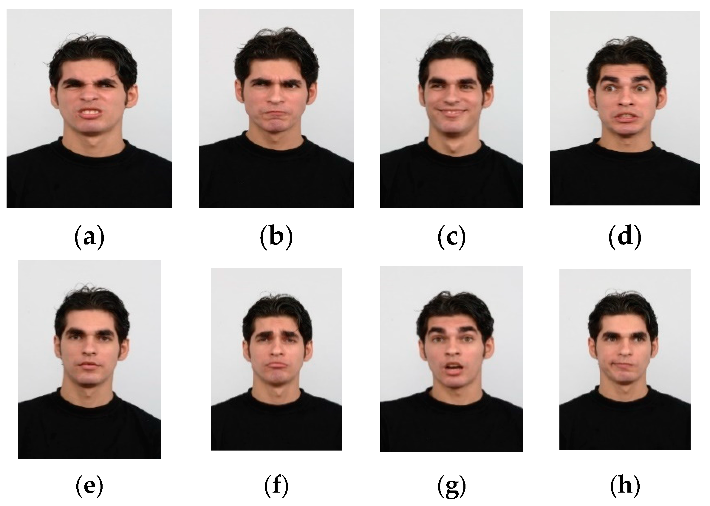
3.1.2. RaFD
3.1.3. Preprocessing
3.2. Feature Description
3.2.1. Histogram of Oriented Gradients
3.2.2. Pyramidal HOG
3.2.3. Gabor Filter
3.2.4. Uniform Local Binary Pattern
3.2.5. Horizontal vertical Neighborhood Local Binary Pattern
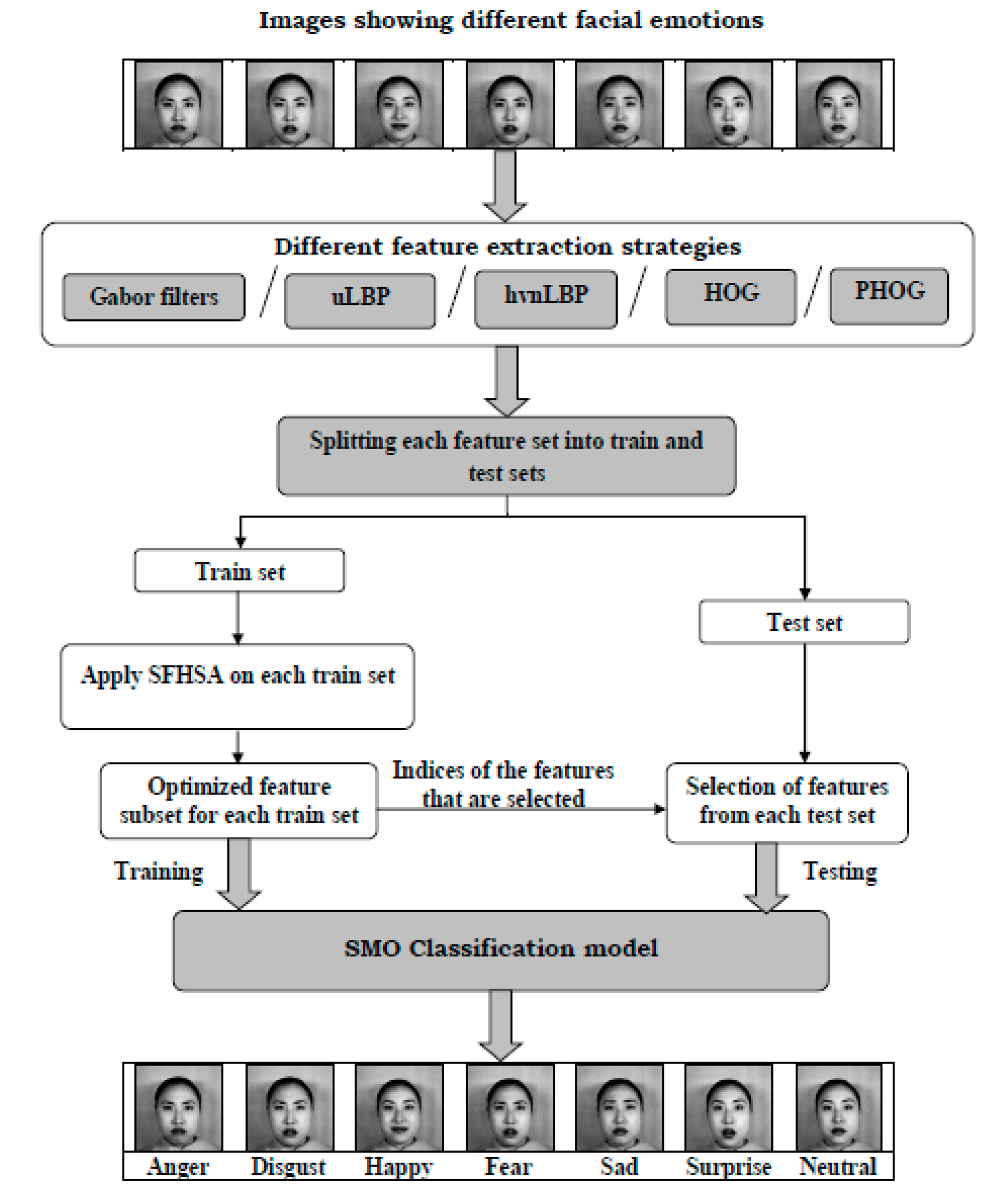
4. Proposed Work
| Algorithm 1 Selection of Optimal Feature Subset using SFHSA |
| 1: Input: Original-feature set 2: Output: Reduced-feature subset 3: User defined parameters: HMS = 15, HMCR = 0.8 and PAR = 0.5 4: Determine the worst feature subset from HM 5: while() { 6: while() { 7: while() { 8: Generate random value for P1 in 9: if() { 10: Choose a feature from the subset 11: Generate a random value for P2 in 12: if() { 13: Generate a random value for in 14: Randomly choose a feature from subset such that cosine similarity is in 15: } 16: } 17: else { 18: Select any feature randomly from the original-feature set 19: } 20: 21: } 22: if( mRMR value of new subset >mRMR value of worst subset) { 23: Replace worst subset with new 24: Find the worst feature subset in the updated HM 25: } 26: 27: } 28: 29: } |
- Harmony Memory Size(HMS)
- Harmony Memory Consideration Rate (HMCR)
- Pitch Adjustment Rate (PAR)
- Number of Iterations
5. Results and Discussion
6. Conclusions
Author Contributions
Funding
Acknowledgments
Conflicts of Interest
References
- Shan, C.; Gong, S.; Mcowan, P.W. Facial expression recognition based on Local Binary Patterns: A comprehensive study. Image Vis. Comput. 2009, 27, 803–816. [Google Scholar] [CrossRef] [Green Version]
- Ekman, P.; Rosenberg, E. What The Face Reveals: Basic and Applied Studies of Spontaneous Expression Using The Facial Action Coding Systems (FACS); Oxford University Press: New York, NY, USA, 1997. [Google Scholar]
- Pantic, M.; Rothkrantz, L.J.M. Automatic analysis of facial expressions: The state of the art. IEEE Trans. Pattern Anal. Mach. Intell. 2000, 22, 1424–1445. [Google Scholar] [CrossRef] [Green Version]
- Happy, S.L.; George, A.; Routray, A. A real time facial expression classification system using Local Binary Patterns. In Proceedings of the 4th International Conference on Intelligent Human Computer Interaction: Advancing Technology for Humanity, IHCI, Kharagpur, India, 27–29 December 2012. [Google Scholar] [CrossRef] [Green Version]
- Silva, L.C.D.E.; Miyasato, I.T. Facial Emotion Recognition Using Multi-modal Information. Electr. Eng. 1997, 1, 9–12. [Google Scholar]
- Zhang, S.; Zhao, X.; Lei, B. Facial Expression Recognition Based on Local Binary Patterns and Local Fisher Discriminant Analysis 2 Local Binary Patterns. Wseas Trans. Signal Process. 2012, 8, 21–31. [Google Scholar]
- Ghosh, M.; Guha, R.; Mondal, R.; Singh, P.K.; Sarkar, R.; Nasipuri, M. Feature selection using histogram-based multi-objective GA for handwritten Devanagari numeral recognition. Adv. Intell. Syst. Comput. 2018, 695, 471–479. [Google Scholar] [CrossRef]
- Malakar, S.; Ghosh, M.; Bhowmik, S.; Sarkar, R.; Nasipuri, M. A GA based hierarchical feature selection approach for handwritten word recognition. Neural Comput. Appl. 2019. [Google Scholar] [CrossRef]
- Belanche, L.A.; González, F.F. Review and Evaluation of Feature Selection Algorithms in Synthetic Problems. arXiv 2011, arXiv:1101.2320. [Google Scholar]
- Dash, M.; Liu, H. Feature selection for classification. Intell. Data Anal. 1997, 1, 131–156. [Google Scholar] [CrossRef]
- Mitra, P.; Murthy, C.A.; Pal, S.K. Unsupervised feature selection using feature similarity. IEEE Trans. Pattern Anal. Mach. Intell. 2002, 24, 301–312. [Google Scholar] [CrossRef]
- Pudil, P.; Novovičová, J.; Kittler, J. Floating search methods in feature selection. Pattern Recognit. Lett. 1994, 15, 1119–1125. [Google Scholar] [CrossRef]
- Sen, S.; Mitra, M.; Bhattacharyya, A.; Sarkar, R.; Schwenker, F.; Roy, K. Feature Selection for Recognition of Online Handwritten Bangla Characters. Neural Process. Lett. 2019. [Google Scholar] [CrossRef]
- Liwicki, M.; Bunke, H. Feature Selection for HMM and BLSTM Based Handwriting Recognition of Whiteboard Notes. Int. J. Pattern Recognit. Artif. Intell. 2009, 23, 907–923. [Google Scholar] [CrossRef]
- Blum, L.; Langley, P. Artificial Intelligence Selection of relevant features and examples in machine. Artif. Intell. 1997, 97, 245–271. [Google Scholar] [CrossRef] [Green Version]
- Guha, R.; Ghosh, M.; Singh, P.K.; Sarkar, R.; Nasipuri, M. M-HMOGA: A new multi-objective feature selection algorithm for handwritten numeral classification. J. Intell. Syst. 2020, 29, 1453–1467. [Google Scholar] [CrossRef]
- Kundu, S.; Paul, S.; Singh, P.K.; Sarkar, R.; Nasipuri, M. Understanding NFC-Net: A deep learning approach to word-level handwritten Indic script recognition. Neural Comput. Appl. 2019, 4. [Google Scholar] [CrossRef]
- Ghosh, M.; Guha, R.; Singh, P.K.; Bhateja, V.; Sarkar, R. A histogram based fuzzy ensemble technique for feature selection. EIntell 2019, 12, 713–724. [Google Scholar] [CrossRef]
- Das, S. Filters, wrappers and a boosting-based hybrid for feature selection. Engineering 2001, 1, 74–81. [Google Scholar]
- Chatterjee, I.; Ghosh, M.; Singh, P.K.; Nasipuri, M. A clustering-based feature selection framework for handwritten Indic script classification. Expert Syst. 2019, 36, e12459. [Google Scholar] [CrossRef]
- Hall, M.A. Correlation-Based Feature Selection for Machine Learning. Ph.D. Thesis, The University of Waikato, Hamilton, New Zeland, 1999. [Google Scholar]
- Ding, C.; Peng, H. Minimum redundancy feature selection from microarray gene expression data. In Proceedings of the 2003 IEEE Bioinformatics Conference. CSB2003, Stanford, CA, USA, 11–14 August 2003. [Google Scholar]
- Diao, R.; Shen, Q. Feature selection with harmony search. IEEE Trans. Syst. ManCybern. Part B Cybern. 2012, 42, 1509–1523. [Google Scholar] [CrossRef]
- Awada, W.; Khoshgoftaar, T.M.; Dittman, D.; Wald, R.; Napolitano, A. A review of the stability of feature selection techniques for bioinformatics data. In Proceedings of the 2012 IEEE 13th International Conference on Information Reuse & Integration (IRI), Las Vegas, NV, USA, 8–10 August 2012. [Google Scholar]
- Lajevardi, S.M.; Hussain, Z.M. Feature selection for facial expression recognition based on optimization algorithm. In Proceedings of the INDS 2009: 2nd International Workshop on Nonlinear Dynamics and Synchronization, Klagenfurt, Austria, 20–21 July 2009; pp. 182–185. [Google Scholar] [CrossRef]
- Guo, G.; Dyer, C.R. Simultaneous feature selection and classifier training via linear programming: A case study for face expression recognition. In Proceedings of the 2003 IEEE Computer Society Conference on Computer Vision and Pattern Recognition 2003, Madison, WI, USA, 18–20 June 2003; Volume 1. [Google Scholar] [CrossRef]
- Gharsalli, S.; Emile, B.; Laurent, H.; Desquesnes, X. Feature Selection for Emotion Recognition based on Random Forest. Visigrapp 2016, 4, 610–617. [Google Scholar] [CrossRef] [Green Version]
- Li, P.; Phung, S.L.; Bouzerdom, A.; Tivive, F.H.C. Feature Selection for Facial Expression Recognition. In Proceedings of the 2010 2nd European Workshop on Visual Information Processing (EUVIP), Paris, France, 5–6 July 2010; pp. 35–40. [Google Scholar] [CrossRef] [Green Version]
- Lajevardi, S.M.; Hussain, Z.M. Automatic facial expression recognition: Feature extraction and selection. SignalImage Video Process. 2012, 6, 159–169. [Google Scholar] [CrossRef]
- Lyons, M.; Akamatsu, S.; Kamachi, M.; Gyoba, J. Coding facial expressions with Gabor wavelets. In Proceedings of the 3rd IEEE International Conference on Automatic Face and Gesture Recognition, FG, Nara, Japan, 14–16 April 1998; pp. 200–205. [Google Scholar] [CrossRef] [Green Version]
- Langner, O.; Dotsch, R.; Bijlstra, G.; Wigboldus, D.H.J.; Hawk, S.T.; van Knippenberg, A. Presentation and validation of the radboud faces database. Cogn. Emot. 2010, 24, 1377–1388. [Google Scholar] [CrossRef]
- Wang, G.; Yang, Y.; Kong, H. Self-Learning facial emotional feature selection based on rough set theory. Math. Probl. Eng. 2009. [Google Scholar] [CrossRef]
- Ghosh, M.; Kundu, T.; Ghosh, D.; Sarkar, R. Feature selection for facial emotion recognition using late hill-climbing based memetic algorithm. Multimed. Tools Appl. 2019, 78, 25753–25779. [Google Scholar] [CrossRef]
- Mistry, L.; Zhang, S.; Neoh, C.; Lim, P.; Fielding, B. A Micro-GA Embedded PSO Feature Selection Approach to Intelligent Facial Emotion Recognition. IEEE Trans. Cybern. 2017, 47, 1496–1509. [Google Scholar] [CrossRef] [Green Version]
- Mlakar, U.; Fister, I.; Brest, J.; Potočnik, B. Multi-Objective Differential Evolution for feature selection in Facial Expression Recognition systems. Expert Syst. Appl. 2017, 89, 129–137. [Google Scholar] [CrossRef]
- Das, S.; Singh, P.K.; Bhowmik, S.; Sarkar, R.; Nasipuri, M. A Harmony Search Based Wrapper Feature Selection Method for Holistic Bangla Word Recognition. arXiv 2017, arXiv:1707.08398. [Google Scholar] [CrossRef] [Green Version]
- Sarkar, S.; Ghosh, M.; Chatterjee, A.; Malakar, S.; Sarkar, R. An advanced particle swarm optimization based feature selection method for tri-script handwritten digit recognition. In Proceedings of the International conference on computational intelligence, communications, and business analytics, Kalyani, India, 27–28 July 2018; pp. 82–94. [Google Scholar]
- Wang, Y.; Liu, Y.; Feng, L.; Zhu, X. Novel feature selection method based on harmony search for email classification. Knowl. Based Syst. 2015, 73, 311–323. [Google Scholar] [CrossRef]
- Zainuddin, Z.; Lai, K.H.; Ong, P. An enhanced harmony search based algorithm for feature selection: Applications in epileptic seizure detection and prediction. Comput. Electr. Eng. 2016, 53, 143–162. [Google Scholar] [CrossRef]
- Bagyamathi, M.; Inbarani, H.H. A Novel Hybridized Rough Set and Improved Harmony Search Based Feature Selection for Protein Sequence Classification. In Big Data in Complex System; Springer: Berlin, Germany, 2015; pp. 173–204. [Google Scholar]
- Wang, Y.; Perez, L. The Effectiveness of Data Augmentation in Image Classification using Deep Learning. arXiv 2017, arXiv:1712.04621. [Google Scholar]
- Viola, P.; Jones, M.J. Robust Real-Time Face Detection. Int. J. Comput. Vis. 2004, 57, 137–154. [Google Scholar] [CrossRef]
- Ghosh, S.; Bhowmik, S.; Ghosh, K.; Sarkar, R.; Chakraborty, S. A filter ensemble feature selection method for handwritten numeral recognition. EMR 2019, 2016, 007213. [Google Scholar]
- Bosch, A.; Zisserman, A.; Munoz, X. Representing shape with a spatial pyramid kernel. In Proceedings of the 6th ACM International Conference on Image and Video Retrieval, CIVR 2007, Amsterdam, The Netherlands, 8 July 2007; pp. 401–408. [Google Scholar] [CrossRef]
- Li, Z.; Imai, J.I.; Kaneko, M. Facial-component-based bag of words and PHOG descriptor for facial expression recognition. In Proceedings of the IEEE International Conference on Systems, Man and Cybernetics, Toronto, ON, Canada, 7–10 October 2009; pp. 1353–1358. [Google Scholar] [CrossRef]
- Ali, M.; Clausi, D. Using The Canny Edge Detector for Feature Extraction and Enhancement of Remote Sensing Images. In Proceedings of the IEEE 2001 International Geoscience and Remote Sensing Symposium, Sydney, Australia, 3–13 July 2001; pp. 2298–2300. [Google Scholar]
- Jana, P.; Ghosh, S.; Sarkar, R.; Nasipuri, M. A Fuzzy C-Means Based Approach Towards Efficient Document Image Binarization. In Proceedings of the Ninth International Conference on Advances in Pattern Recognition, ICAPR 2017, Bangalore, India, 27–30 December 2017; pp. 1–6. [Google Scholar]
- Jain, K.; Farrokhnia, F. Unsupervised texture segmentation using Gabor filters. Pattern Recognit. 1991, 24, 1167–1186. [Google Scholar] [CrossRef] [Green Version]
- Liu, X.; Wechsler, H. Gabor feature based classification using the enhanced Fisher linear discriminant model for face recognition. IEEE Trans. Image Process. 2002, 11, 467–476. [Google Scholar] [CrossRef] [Green Version]
- Ou, J.; Bai, X.-B.; Pei, Y.; Ma, L.; Liu, W. Automatic Facial Expression Recognition Using Gabor Filter and Expression Analysis. In Proceedings of the 2010 Second International Conference on Computer Modeling and Simulation, Sanyan, China, 22–24 January 2010; pp. 215–218. [Google Scholar] [CrossRef]
- Ojala, T.; Pietikäinen, M.; Mäenpää, T. Multiresolution gray-scale and rotation invariant texture classification with local binary patterns. IEEE Trans. Pattern Anal. Mach. Intell. 2002, 24, 971–987. [Google Scholar] [CrossRef]
- Kim, J.H. Harmony Search Algorithm: A Unique Music-inspired Algorithm. Procedia Eng. 2016, 154, 1401–1405. [Google Scholar] [CrossRef] [Green Version]
- Lee, K.S.; Geem, Z.W. A new structural optimization method based on the harmony search algorithm. Comput. Struct. 2004, 82, 781–798. [Google Scholar] [CrossRef]
- Geem, Z.W.; Kim, J.H.; Loganathan, G.V. A New Heuristic Optimization Algorithm: Harmony Search. Optimization 2001, 35–54. [Google Scholar] [CrossRef]
- Geem, Z.W. Optimal cost design of water distribution networks using harmony search. Eng. Optim. 2006, 38, 259–277. [Google Scholar] [CrossRef]
- Mahdavi, M.; Fesanghary, M.; Damangir, E. An improved harmony search algorithm for solving optimization problems. Appl. Math. Comput. 2007, 188, 1567–1579. [Google Scholar] [CrossRef]
- Pratap, V.; Tomar, S.; Dwivedi, D.; Gwalior, M. Ansys Modelling and Simulation of Temperature. Int. J. Adv. Eng. Res. Dev. 2015, 2015, 1–4. [Google Scholar]
- Peng, H.; Long, F.; Ding, C. Multi-label feature selection based on mutual information. In Proceedings of the ICNC-FSKD 2018—14th International Conference on Natural Computing Fuzzy Systems Knowledge Discovery, Huangshan, China, 28–30 July 2018; pp. 1379–1386. [Google Scholar] [CrossRef]
- Radovic, M.; Ghalwash, M.; Filipovic, N.; Obradovic, Z. Minimum redundancy maximum relevance feature selection approach for temporal gene expression data. BMC Bioinform. 2017, 18, 1–14. [Google Scholar] [CrossRef] [PubMed] [Green Version]
- Sakar, C.O.; Kursun, O.; Gurgen, F. A feature selection method based on kernel canonical correlation analysis and the minimum Redundancy-Maximum Relevance filter method. Expert Syst. Appl. 2012, 39, 3432–3437. [Google Scholar] [CrossRef]
- Senawi, A.; Wei, H.L.; Billings, S.A. A new maximum relevance-minimum multicollinearity (MRmMC) method for feature selection and ranking. Pattern Recognit. 2017, 67, 47–61. [Google Scholar] [CrossRef]
- Pearson’s Correlation Coefficient Definition. In Encyclopedia of Public Health; Springer: Berlin, Germany, 2008; p. 1172. [CrossRef]
- Wei, J.; Zhang, R.; Yu, Z.; Hu, R.; Tang, J.; Gui, C.; Yuan, Y. A BPSO-SVM algorithm based on memory renewal and enhanced mutation mechanisms for feature selection. Appl. Soft Comput. J. 2017, 58, 176–192. [Google Scholar] [CrossRef]
- Mafarja, M.; Mirjalili, S. Whale optimization approaches for wrapper feature selection. Appl. Soft Comput. J. 2018, 62, 441–453. [Google Scholar] [CrossRef]


| Image Dimension | Feature Dimension | Final Feature Dimension after down Sampling |
|---|---|---|
| Feature Descriptor | Dataset | Dimension of Facial Images | Size of the Original-Feature Vector | Accuracy Score (%) | Size of the Optimal Feature Vector Obtained by SFHSA [Reduction in %] | Accuracy Score (%)[Change in %] |
|---|---|---|---|---|---|---|
| uLBP | JAFFE | 32 × 32 | 944 | 62.34 | 570[60.38%] | 78.95[+16.61%] |
| 48 × 48 | 62.34 | 339[35.91%] | 75.32[+12.98%] | |||
| 64 × 64 | 59.74 | 541[57.31%] | 74.13[+14.39%] | |||
| RaFD | 32 × 32 | 83.58 | 608[64.41%] | 87.75[+4.17%] | ||
| 48 × 48 | 88.62 | 445[47.14%] | 85.48[−3.14%] | |||
| 64 × 64 | 86.38 | 573[60.70%] | 92.16[+5.78%] | |||
| hvnLBP | JAFFE | 32 × 32 | 4096 | 57.14 | 1380[33.69%] | 67.41[+10.27%] |
| 48 × 48 | 46.75 | 1416[34.57%] | 55.84[+12.09%] | |||
| 64 × 64 | 44.16 | 1433[34.99%] | 67.42[+23.26%] | |||
| RaFD | 32 × 32 | 66.42 | 1513[36.94%] | 72.39[+5.97%] | ||
| 48 × 48 | 74.07 | 1493[36.45%] | 75.74[+1.37%] | |||
| 64 × 64 | 69.4 | 1494[36.47%] | 75.81[+6.41%] | |||
| Gabor | JAFFE | 32 × 32 | 640 | 67.53 | 197[30.78%] | 81.82[+14.29%] |
| 48 × 48 | 1440 | 72.73 | 560[38.89%] | 92.21[+19.48%] | ||
| 64 × 64 | 2560 | 71.43 | 818[31.95%] | 90.91[+19.48%] | ||
| RaFD | 32 × 32 | 640 | 90.49 | 241[37.66%] | 91.91[+1.42%] | |
| 48 × 48 | 1440 | 95.71 | 341[23.68%] | 96.51[+0.8%] | ||
| 64 × 64 | 2560 | 98.51 | 462[18.04%] | 97.79[−0.72%] | ||
| HOG | JAFFE | 32 × 32 | 324 | 71.43 | 189[58.33%] | 87.94[+16.51%] |
| 48 × 48 | 900 | 74.03 | 403[44.78%] | 92.21[+18.18%] | ||
| 64 × 64 | 1764 | 71.43 | 1411[79.99%] | 85.71[+14.28%] | ||
| RaFD | 32 × 32 | 324 | 88.43 | 205[63.27%] | 89.15[+0.72%] | |
| 48 × 48 | 900 | 94.22 | 385[42.78%] | 95.40[+1.18%] | ||
| 64 × 64 | 1764 | 93.66 | 544[30.83%] | 96.32[+2.66%] | ||
| PHOG | JAFFE | 32 × 32 | 680 | 53.25 | 321[47.21%] | 76.32[+20.07%] |
| 48 × 48 | 66.23 | 408[60.00%] | 85.27[+19.04%] | |||
| 64 × 64 | 59.74 | 409[60.15%] | 84.39[+24.65%] | |||
| RaFD | 32 × 32 | 78.54 | 429[63.09%] | 85.01[+6.17%] | ||
| 48 × 48 | 85.45 | 271[39.85%] | 89.03[+3.58%] | |||
| 64 × 64 | 88.81 | 300[44.12%] | 88.30[−0.51%] |
| Dataset | Image Size | No FS | SA | GA | MA | ||||
| Feature Dimension | Accuracy Score (%) | Feature Dimension | Accuracy Score (%) | Feature Dimension | Accuracy Score (%) | Feature Dimension | Accuracy Score (%) | ||
| JAFFE | 32 × 32 | 944 | 62.34 | 481 | 37.66 | 661 | 71.43 | 542 | 76.62 |
| 48 × 48 | 62.34 | 487 | 45.45 | 678 | 79.22 | 672 | 76.62 | ||
| 64 × 64 | 59.74 | 493 | 45.45 | 611 | 70.13 | 703 | 71.43 | ||
| RAFD | 32 × 32 | 83.58 | 485 | 69.40 | 791 | 86.38 | 716 | 86.75 | |
| 48 × 48 | 88.62 | 441 | 78.73 | 696 | 92.16 | 696 | 91.47 | ||
| 64 × 64 | 86.38 | 487 | 76.49 | 677 | 90.11 | 554 | 91.42 | ||
| Dataset | ME-BPSO | WAO-CM | LHCMA | SFHSA | |||||
| Feature Dimension | Accuracy Score (%) | Feature Dimension | Accuracy Score (%) | Feature Dimension | Accuracy Score (%) | Feature Dimension | Accuracy Score (%) | ||
| JAFFE | 576 | 64.93 | 911 | 61.04 | 594 | 76.62 | 570 | 78.95 | |
| 472 | 62.34 | 670 | 74.03 | 574 | 76.62 | 339 | 75.32 | ||
| 603 | 72.34 | 869 | 63.64 | 570 | 74.03 | 541 | 74.13 | ||
| RAFD | 620 | 78.17 | 915 | 82.28 | 600 | 87.13 | 608 | 87.75 | |
| 533 | 84.89 | 883 | 92.72 | 552 | 91.61 | 445 | 85.48 | ||
| 638 | 83.40 | 821 | 86.01 | 555 | 90.30 | 573 | 92.16 | ||
| Dataset | Image Size | No FS | SA | GA | MA | ||||
|---|---|---|---|---|---|---|---|---|---|
| Feature Dimension | Accuracy Score (%) | Feature Dimension | Accuracy Score (%) | Feature Dimension | Accuracy Score (%) | Feature Dimension | Accuracy Score (%) | ||
| JAFFE | 32 × 32 | 4096 | 57.14 | 2059 | 51.95 | 2613 | 70.13 | 2232 | 70.13 |
| 48 × 48 | 46.75 | 2011 | 42.86 | 2284 | 61.04 | 2451 | 58.44 | ||
| 64 × 64 | 44.16 | 2132 | 38.96 | 2254 | 57.14 | 2208 | 58.44 | ||
| RAFD | 32 × 32 | 66.42 | 2024 | 61.19 | 2721 | 70.15 | 2081 | 72.01 | |
| 48 × 48 | 74.07 | 2049 | 68.10 | 2580 | 75.00 | 2584 | 76.49 | ||
| 64 × 64 | 69.4 | 2026 | 64.18 | 2457 | 72.76 | 2090 | 74.44 | ||
| Dataset | ME-BPSO | WAO-CM | LHCMA | SFHSA | |||||
| Feature Dimension | Accuracy Score (%) | Feature Dimension | Accuracy Score (%) | Feature Dimension | Accuracy Score (%) | Feature Dimension | Accuracy Score (%) | ||
| JAFFE | 2118 | 61.04 | 3894 | 61.04 | 2235 | 72.73 | 1380 | 67.41 | |
| 1975 | 50.65 | 2921 | 51.95 | 2158 | 63.64 | 1416 | 55.84 | ||
| 2595 | 50.65 | 1469 | 54.55 | 2060 | 58.44 | 1433 | 67.42 | ||
| RAFD | 2758 | 66.98 | 3772 | 70.71 | 2211 | 70.34 | 1513 | 72.39 | |
| 2615 | 72.57 | 3489 | 77.61 | 2279 | 75.19 | 1493 | 75.74 | ||
| 2584 | 69.22 | 3914 | 75.56 | 2383 | 73.69 | 1494 | 75.81 | ||
| Dataset | Image Size | No FS | SA | GA | MA | |||||
|---|---|---|---|---|---|---|---|---|---|---|
| Feature Dimension | Accuracy Score (%) | Feature Dimension | Accuracy Score (%) | Feature Dimension | Accuracy Score (%) | Feature Dimension | Accuracy Score (%) | |||
| JAFFE | 32 × 32 | 640 | 67.53 | 323 | 66.23 | 375 | 79.22 | 377 | 84.42 | |
| 48 × 48 | 1440 | 72.73 | 704 | 68.83 | 910 | 80.52 | 836 | 84.42 | ||
| 64 × 64 | 2560 | 71.43 | 1293 | 71.43 | 1541 | 81.82 | 1408 | 83.12 | ||
| RAFD | 32 × 32 | 640 | 90.49 | 320 | 83.21 | 400 | 93.28 | 429 | 94.03 | |
| 48 × 48 | 1440 | 95.71 | 683 | 91.60 | 851 | 98.32 | 894 | 98.88 | ||
| 64 × 64 | 2560 | 98.51 | 1333 | 95.90 | 1613 | 98.32 | 1414 | 98.75 | ||
| Dataset | ME-BPSO | WAO-CM | LHCMA | SFHSA | ||||||
| Feature Dimension | Accuracy Score (%) | Feature Dimension | Accuracy Score (%) | Feature Dimension | Accuracy Score (%) | Feature Dimension | Accuracy Score (%) | |||
| JAFFE | 301 | 84.03 | 217 | 79.22 | 319 | 84.42 | 197 | 81.82 | ||
| 701 | 84.42 | 630 | 83.12 | 767 | 83.12 | 560 | 92.21 | |||
| 1557 | 83.12 | 419 | 89.61 | 1428 | 83.12 | 818 | 90.91 | |||
| RAFD | 344 | 92.36 | 557 | 93.74 | 337 | 94.59 | 241 | 91.91 | ||
| 770 | 95.52 | 1074 | 96.46 | 758 | 98.88 | 341 | 96.51 | |||
| 1300 | 98.13 | 1186 | 97.01 | 1271 | 99.25 | 462 | 97.79 | |||
| Dataset | Image Size | No FS | SA | GA | MA | ||||
|---|---|---|---|---|---|---|---|---|---|
| Feature Dimension | Accuracy Score (%) | Feature Dimension | Accuracy Score (%) | Feature Dimension | Accuracy Score (%) | Feature Dimension | Accuracy Score (%) | ||
| JAFFE | 32 × 32 | 324 | 71.43 | 178 | 70.13 | 195 | 85.71 | 206 | 83.12 |
| 48 × 48 | 900 | 74.03 | 444 | 67.53 | 530 | 89.61 | 507 | 87.01 | |
| 64 × 64 | 1764 | 71.43 | 887 | 58.44 | 1097 | 80.52 | 1105 | 83.12 | |
| RAFD | 32 × 32 | 324 | 88.43 | 143 | 85.74 | 186 | 92.16 | 167 | 92.16 |
| 48 × 48 | 900 | 94.22 | 538 | 91.54 | 480 | 97.01 | 390 | 97.01 | |
| 64 × 64 | 1764 | 93.66 | 816 | 92.66 | 867 | 96.27 | 675 | 96.27 | |
| Dataset | ME-BPSO | WAO-CM | LHCMA | SFHSA | |||||
| Feature Dimension | Accuracy Score (%) | Feature Dimension | Accuracy Score (%) | Feature Dimension | Accuracy Score (%) | Feature Dimension | Accuracy Score (%) | ||
| JAFFE | 195 | 82.32 | 281 | 81.03 | 182 | 87.01 | 189 | 87.94 | |
| 440 | 85.32 | 371 | 88.22 | 482 | 89.61 | 403 | 92.21 | ||
| 923 | 82.12 | 1446 | 81.62 | 1008 | 83.12 | 1411 | 85.71 | ||
| RAFD | 211 | 85.07 | 295 | 86.94 | 160 | 92.35 | 205 | 89.15 | |
| 530 | 93.91 | 605 | 93.47 | 455 | 97.20 | 385 | 95.40 | ||
| 1039 | 95.15 | 1041 | 94.96 | 800 | 97.57 | 544 | 96.32 | ||
| Dataset | Image Size | No FS | SA | GA | MA | ||||
|---|---|---|---|---|---|---|---|---|---|
| Feature Dimension | Accuracy Score (%) | Feature Dimension | Accuracy Score (%) | Feature Dimension | Accuracy Score (%) | Feature Dimension | Accuracy Score (%) | ||
| JAFFE | 32 × 32 | 680 | 53.25 | 357 | 46.75 | 419 | 64.94 | 374 | 68.83 |
| 48 × 48 | 66.23 | 344 | 58.44 | 396 | 81.82 | 405 | 80.52 | ||
| 64 × 64 | 59.74 | 342 | 62.34 | 423 | 79.22 | 412 | 79.22 | ||
| RAFD | 32 × 32 | 78.54 | 351 | 75.19 | 489 | 82.46 | 416 | 84.14 | |
| 48 × 48 | 85.45 | 354 | 84.89 | 398 | 90.49 | 344 | 91.98 | ||
| 64 × 64 | 88.81 | 366 | 87.87 | 411 | 91.23 | 364 | 93.84 | ||
| Dataset | ME-BPSO | WAO-CM | LHCMA | SFHSA | |||||
| Feature Dimension | Accuracy Score (%) | Feature Dimension | Accuracy Score (%) | Feature Dimension | Accuracy Score (%) | Feature Dimension | Accuracy Score (%) | ||
| JAFFE | 361 | 63.64 | 633 | 59.74 | 359 | 72.73 | 321 | 76.32 | |
| 440 | 71.43 | 441 | 67.53 | 373 | 80.52 | 408 | 85.27 | ||
| 334 | 74.03 | 178 | 71.43 | 374 | 81.82 | 409 | 84.39 | ||
| RAFD | 420 | 78.92 | 491 | 80.41 | 396 | 83.21 | 429 | 85.01 | |
| 391 | 87.87 | 541 | 90.11 | 331 | 91.04 | 271 | 89.03 | ||
| 352 | 90.67 | 503 | 92.35 | 395 | 93.10 | 300 | 88.30 | ||
| WAO-CM | LHCMA | SFHSA | ||||||||
|---|---|---|---|---|---|---|---|---|---|---|
| Dataset | Image Size | Precision | Recall | F-Measure | PRECISION | Recall | F-Measure | Precision | Recall | F-Measure |
| JAFFE | 32 × 32 | 0.613 | 0.610 | 0.611 | 0.767 | 0.766 | 0.766 | 0.797 | 0.789 | 0.791 |
| 48 × 48 | 0.738 | 0.740 | 0.739 | 0.765 | 0.766 | 0.765 | 0.757 | 0.753 | 0.753 | |
| 64 × 64 | 0.634 | 0.636 | 0.635 | 0.743 | 0.740 | 0.741 | 0.750 | 0.741 | 0.742 | |
| RaFD | 32 × 32 | 0.826 | 0.823 | 0.825 | 0.870 | 0.871 | 0.871 | 0.875 | 0.878 | 0.877 |
| 48 × 48 | 0.930 | 0.927 | 0.928 | 0.918 | 0.916 | 0.917 | 0.853 | 0.855 | 0.853 | |
| 64 × 64 | 0.857 | 0.860 | 0.859 | 0.906 | 0.903 | 0.905 | 0.928 | 0.921 | 0.923 | |
| WAO-CM | LHCMA | SFHSA | ||||||||
|---|---|---|---|---|---|---|---|---|---|---|
| Dataset | Image Size | Precision | Recall | F-Measure | Precision | Recall | F-Measure | Precision | Recall | F-Measure |
| JAFFE | 32 × 32 | 0.609 | 0.610 | 0.609 | 0.725 | 0.727 | 0.727 | 0.680 | 0.674 | 0.675 |
| 48 × 48 | 0.523 | 0.520 | 0.521 | 0.635 | 0.636 | 0.635 | 0.561 | 0.558 | 0.559 | |
| 64 × 64 | 0.548 | 0.546 | 0.546 | 0.587 | 0.584 | 0.585 | 0.667 | 0.674 | 0.672 | |
| RaFD | 32 × 32 | 0.710 | 0.707 | 0.709 | 0.708 | 0.703 | 0.706 | 0.721 | 0.724 | 0.723 |
| 48 × 48 | 0.773 | 0.776 | 0.775 | 0.748 | 0.752 | 0.749 | 0.766 | 0.757 | 0.760 | |
| 64 × 64 | 0.757 | 0.756 | 0.756 | 0.740 | 0.737 | 0.737 | 0.757 | 0.758 | 0.757 | |
| WAO-CM | LHCMA | SFHSA | ||||||||
|---|---|---|---|---|---|---|---|---|---|---|
| Dataset | Image Size | Precision | Recall | F-Measure | Precision | Recall | F-Measure | Precision | Recall | F-Measure |
| JAFFE | 32 × 32 | 0.797 | 0.792 | 0.794 | 0.847 | 0.844 | 0.845 | 0.821 | 0.818 | 0.819 |
| 48 × 48 | 0.827 | 0.831 | 0.831 | 0.836 | 0.831 | 0.833 | 0.927 | 0.922 | 0.924 | |
| 64 × 64 | 0.898 | 0.896 | 0.897 | 0.827 | 0.831 | 0.830 | 0.913 | 0.909 | 0.910 | |
| RaFD | 32 × 32 | 0.939 | 0.937 | 0.938 | 0.949 | 0.946 | 0.946 | 0.923 | 0.919 | 0.920 |
| 48 × 48 | 0.971 | 0.965 | 0.968 | 0.991 | 0.989 | 0.989 | 0.973 | 0.965 | 0.966 | |
| 64 × 64 | 0.968 | 0.970 | 0.969 | 0.989 | 0.992 | 0.990 | 0.986 | 0.978 | 0.982 | |
| WAO-CM | LHCMA | SFHSA | ||||||||
|---|---|---|---|---|---|---|---|---|---|---|
| Dataset | Image Size | Precision | Recall | F-Measure | Precision | Recall | F-Measure | Precision | Recall | F-Measure |
| JAFFE | 32 × 32 | 0.808 | 0.810 | 0.809 | 0.864 | 0.870 | 0.868 | 0.875 | 0.879 | 0.876 |
| 48 × 48 | 0.886 | 0.882 | 0.883 | 0.898 | 0.896 | 0.897 | 0.929 | 0.922 | 0.924 | |
| 64 × 64 | 0.817 | 0.816 | 0.816 | 0.835 | 0.831 | 0.832 | 0.863 | 0.857 | 0.859 | |
| RaFD | 32 × 32 | 0.865 | 0.869 | 0.868 | 0.926 | 0.924 | 0.924 | 0.894 | 0.891 | 0.892 |
| 48 × 48 | 0.938 | 0.935 | 0.937 | 0.970 | 0.972 | 0.971 | 0.960 | 0.954 | 0.956 | |
| 64 × 64 | 0.953 | 0.950 | 0.951 | 0.973 | 0.976 | 0.974 | 0.961 | 0.963 | 0.962 | |
| WAO-CM | LHCMA | SFHSA | ||||||||
|---|---|---|---|---|---|---|---|---|---|---|
| Dataset | Image Size | Precision | Recall | F-Measure | Precision | Recall | F-Measure | Precision | Recall | F-Measure |
| JAFFE | 32 × 32 | 0.601 | 0.597 | 0.599 | 0.725 | 0.727 | 0.726 | 0.762 | 0.763 | 0.762 |
| 48 × 48 | 0.672 | 0.675 | 0.674 | 0.802 | 0.805 | 0.803 | 0.856 | 0.853 | 0.853 | |
| 64 × 64 | 0.718 | 0.714 | 0.716 | 0.820 | 0.818 | 0.818 | 0.845 | 0.844 | 0.844 | |
| RaFD | 32 × 32 | 0.806 | 0.804 | 0.804 | 0.835 | 0.832 | 0.834 | 0.861 | 0.850 | 0.851 |
| 48 × 48 | 0.900 | 0.901 | 0.900 | 0.912 | 0.910 | 0.911 | 0.894 | 0.890 | 0.892 | |
| 64 × 64 | 0.927 | 0.924 | 0.925 | 0.937 | 0.931 | 0.933 | 0.885 | 0.883 | 0.883 | |
© 2020 by the authors. Licensee MDPI, Basel, Switzerland. This article is an open access article distributed under the terms and conditions of the Creative Commons Attribution (CC BY) license (http://creativecommons.org/licenses/by/4.0/).
Share and Cite
Saha, S.; Ghosh, M.; Ghosh, S.; Sen, S.; Singh, P.K.; Geem, Z.W.; Sarkar, R. Feature Selection for Facial Emotion Recognition Using Cosine Similarity-Based Harmony Search Algorithm. Appl. Sci. 2020, 10, 2816. https://doi.org/10.3390/app10082816
Saha S, Ghosh M, Ghosh S, Sen S, Singh PK, Geem ZW, Sarkar R. Feature Selection for Facial Emotion Recognition Using Cosine Similarity-Based Harmony Search Algorithm. Applied Sciences. 2020; 10(8):2816. https://doi.org/10.3390/app10082816
Chicago/Turabian StyleSaha, Soumyajit, Manosij Ghosh, Soulib Ghosh, Shibaprasad Sen, Pawan Kumar Singh, Zong Woo Geem, and Ram Sarkar. 2020. "Feature Selection for Facial Emotion Recognition Using Cosine Similarity-Based Harmony Search Algorithm" Applied Sciences 10, no. 8: 2816. https://doi.org/10.3390/app10082816