An Improved Circumferential Fourier Fit (CFF) Method for Blade Tip Timing Measurements


State Key Laboratory of Precision Measuring Technology and Instruments, Tianjin University, Weijin Road, Tianjin 300072, China
*
Author to whom correspondence should be addressed.
Appl. Sci. 2020, 10(11), 3675; https://doi.org/10.3390/app10113675
Submission received: 7 May 2020
/
Revised: 19 May 2020
/
Accepted: 20 May 2020
/
Published: 26 May 2020
(This article belongs to the Special Issue Manufacturing Metrology)
Abstract
:Rotating blade vibration measurements are very important for any turbomachinery research and development program. The blade tip timing (BTT) technique uses the time of arrival (ToA) of the blade tip passing the casing mounted probes to give the blade vibration. As a non-contact technique, BTT is necessary for rotating blade vibration measurements. The higher accuracy of amplitude and vibration frequency identification has been pursued since the development of BTT. An improved circumferential Fourier fit (ICFF) method is proposed. In this method, the ToA is not only dependent on the rotating speed and monitoring position, but also on blade vibration. Compared with the traditional circumferential Fourier fit (TCFF) method, this improvement is more consistent with reality. A 12-blade assembly simulator and experimental data were used to evaluate the ICFF performance. The simulated results showed that the ICFF performance is comparable to TCFF in terms of EO identification, except the lower PSR or more number probes that have a more negative effect on ICFF. Besides, the accuracy of amplitude identification is higher for ICFF than TCFF on all test conditions. Meanwhile, the higher accuracy of the reconstruction of ICFF was further verified in all measurement resonance analysis.
1. Introduction
Rotating blade vibration measurements are of great significance for any turbomachinery research and development program [1,2,3,4]. As a non-contact measurement technique, the blade tip timing (BTT) technique has been widely used in blade vibration measurements, such as in aero-engines, turbines, and compressors [5,6,7,8,9]. This technique uses the time of arrival (ToA) of the blade tip passing the casing-mounted probes to give the blade vibration. Compared with traditional strain gauges [10], BTT has the advantages of low equipment cost, easy installation, and monitoring vibration of each blade that passes through the probe [11]. However, BTT signals are typically under-sampled. It brings difficulty for blade vibration analysis.
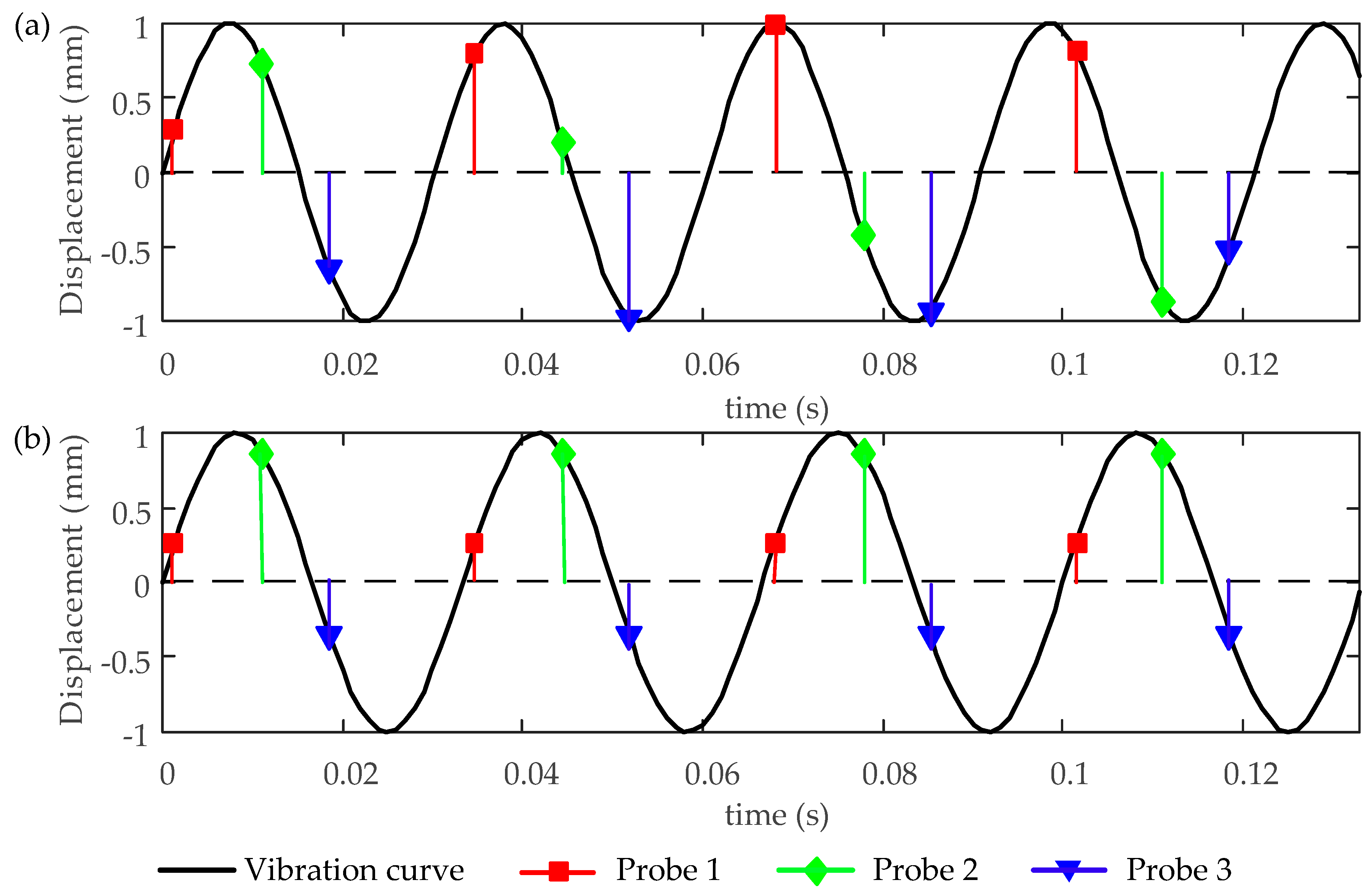
In BTT analysis, the character of the blade response is usually grouped into two distinct classes, namely, asynchronous vibration and synchronous vibration. Asynchronous vibration mainly occurs in the abnormal vibrations, such as rotating stall, surge, flutter, and bearing vibration [12,13,14]. In these cases, the blade vibration frequency is a non-integer multiple of the rotating frequency and the phase of the response can be arbitrary, which is shown in Figure 1a. Synchronous vibration is excited by the multiples of the rotating frequency [15,16]. At constant speed, the probe can only monitor the blade response at a fixed point since the phase of the response remains fixed relative to a stationary datum at a given speed. The under-sampling of synchronous vibration is shown in Figure 1b. Therefore, the degree of under-sampling is much higher for synchronous vibration, which leads to more difficultly in identifying the blade vibration parameters from raw data.
Up to now, the identification methods for BTT signals are divided into two categories; one is spectrum analysis and the other is curve fitting. The spectrum analysis method generally maps BTT signals to frequency domain space to obtain information about blade vibration. This type of method usually requires that the sampling frequency is kept constant, that is, the signal is sampled on a constant rotating speed. Spectrum analysis methods mainly include a traveling wave analysis (TW) [17], the “5 + 2” method [18], the minimum variance spectrum estimation (MVSE) [19], non-uniform discrete Fourier transform (NUDFT) [20], cross-spectrum estimation (CSE) [21], sparse reconstruction (SR) method [22], etc. The spectrum method mainly is used to analyze asynchronous vibration. However, the results of spectrum analysis are always corrupted with aliases and replicas of the true frequency components. Consequently, the real spectrum recovery needs to further make use of the knowledge of the blade’s dynamic properties, which is usually obtained based on the finite element method (FEM) [23]. The curve fitting method usually uses sine functions to fit the blade vibration displacements, which are obtained by speed sweeping through the resonance region. The curve fitting method mainly used to analyze synchronous vibration. These methods mainly include the single-parameter method [24], the two-parameter plot method [25], autoregressive (AR) method [26,27], the circumferential Fourier fit (CFF) method [28], the method without once per revolution [29,30], and so on. The accuracy of these curve fitting methods is often related to the amount of fitted data and the inter-blade coupling of the mistuned blade.
The CFF method is highly recommended for synchronous vibration analysis by Hood Technology Corporation, which is a commercial vendor of BTT systems [28]. This method can identify the amplitude and phase of vibration on the conditions that the engine order (EO) is known. Tao Ouyang proposed a traversed EO method based on CFF, which is no longer limited to known EO [31]. In this paper, we refer to the Ouyang CFF as the traditional CFF (TCFF). An improved formulation for the calculation of the TOA was proposed by S. Heath and M. Imregun, who proved the BTT analysis technique has limitations regarding synchronous response, in that the blade vibration was not considered in the TOA [32]. In this paper, an improved CFF (ICFF) method is proposed, which considers the influence of blade vibration when measuring the ToA of the blade tip. The ICFF is more robust with more probes employed to complete the parameter identification rather than the single-parameters or the improved single-parameters method that just used one probe. Compared to the AR method that requests the probes are equally spaced installed, the ICFF method has not got so strict limitations for probe layout. Moreover, the ICFF introduced into the EO traversed thought that proposed by the literature [31] and a more precision calculation method proposed by the literature [32]. These improvements are more consistent with reality. A 12-blade assembly simulator and experimental data were used to evaluate the performance of ICFF. In both simulated and experimental tests, the ICFF performed better than TCFF.
2. The Improved Circumferential Fourier Fit (ICFF) Method
2.1. A Brief Introduction to TCFF
The theory of TCFF is consistent with the CFF method. It uses multiple sensors (usually four) distributed at different positions in the circumferential direction of the casing to monitor blade vibration. On the condition that the EO is known, TCFF is equivalent to the CFF method, and the blade vibration parameters can be directly calculated according to the CFF method. In the case that the EO is unknown, the blade amplitude, vibration phase, direct current offset, and fitting residual error are calculated using the CFF method with each possible EO, which is selected within a certain range. After the traversal is completed, according to the principle of least squares, the EO corresponding to the minimum fitting residual error is the true EO, and the blade vibration parameters calculated using this EO are the true vibration parameters. More details about TCFF are provided by the literature [31]. The TCFF method introduces the idea of EO traversal to overcome the shortcomings of CFF, which must rely on known EO to identify blade vibration. Although TCFF did not make any changes to the CFF theoretical method, except to introduce EO traversal, to a certain extent, TCFF has wider engineering applicability than the CFF method. However, neither TCFF nor the CFF method takes into account the influence of blade vibration on the ToA. The ICFF method proposed in this paper further considers the effect of blade vibration on the ToA to achieve a higher accuracy of blade amplitude identification. Considering that TCFF can perform EO traversal, which overcomes the disadvantage that CFF must rely on known EO, this paper uses TCFF as a comparison object to illustrate the performance improvement of ICFF.
2.2. The Theoretical Basis of ICFF
Assuming the blade response is of single-frequency vibration:
where y represents the vibration displacement of the blade tip, A represents the amplitude, ω represents the angular frequency, t represents the ToA, ϕ represents the phase, and d represents the direct current offset. For the synchronous vibration, there is:
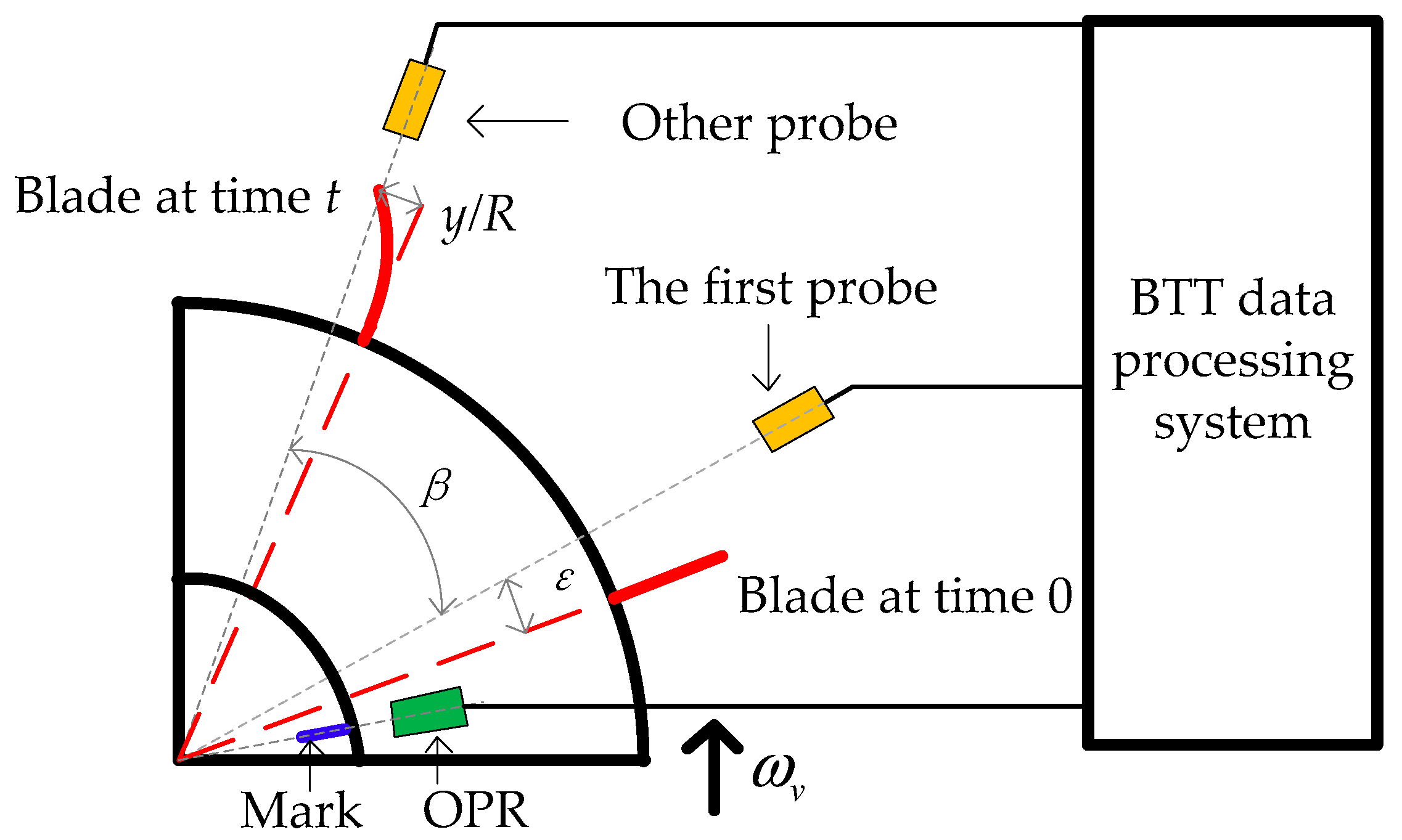
where ωv represents the rotor rotating frequency. This is based on the BTT measurement principle, assuming that the blade rotates to the monitoring position β at time t. The geometry relationship between the rotation angular, monitoring position, and blade vibration is shown in Figure 2. The equivalence relationship can be given by:
where is the average rotating speed, and n is the number of revolution. In the Equation (3), it can be seen that the time t (that is ToA) is not only dependent on the rotating speed and monitoring position, but also on the blade vibration.
Let:
According to Equations (1)–(4), the blade vibration displacement monitored by the probe mounted at the position β can be given:
Equation (5) is the mathematical model for monitoring the vibration displacement of the blade tip under the influence of blade vibration that is considered. According to the literature [32], in the case of large vibration displacement or mistuning, the improved single-parameter method that considers the influence of blade vibration has higher accuracy than the traditional method. ICFF is a combination of the theory of the improved single-parameter method and TCFF.
2.3. The Derivation of ICFF
Equation (5) is transformed by triangle formulas:
TCFF usually needs at least four probes to monitor blade vibration. In this section, assuming that there are g probes, the blade vibration displacement sequence can be represented according to Equation (6):
That is:
where Y is the displacement vector, B is the coefficient matrix, and X is the parameter matrix. The main difference between ICFF and TCFF is the constituent parameters of the coefficient matrix B, although Equation (7) in this paper is the same in form as TCFF. For the TCFF method, the coefficient matrix B is completely determined by the probe mounted position β and the initial angle ε, that is, once the probe installation scheme is determined, the coefficient matrix B is also determined. This means that the coefficient matrix B is a constant in the TCFF method. The same applies to the CFF method. However, the coefficient matrix B in ICFF is a function of three parameters: the probe installation angle β, the initial angle ε, and the blade vibration displacement y/R. According to the derivation in Section 2.2, blade vibration displacement is also one of the most important parameters affecting the ToA. In this case, the coefficient matrix B is no longer a constant but can be adjusted in real-time according to the actual vibration displacement of the blade.
Based on the principle of least squares and EO traversal, when the possible engine order EOk (k = 1, 2, 3…) is selected, there is:
The condition number is the indicator of the quality of the matrix B, which influence the accuracy of X directly. The larger the condition number, the more ill-condition matrix B is, and the more sensitive of the calculated results are to the measurement error. An effective way to improve the quality of the matrix B is to adjust the sensor layout. Therefore, based on the minimization the condition number of matrix B, a method about determining the sensor layout can be derived. The condition number mentioned above and the probe spacing of the resonance (PSR) used later in the paper as an indicator of sensor distribution both are methods essentially to determine how the sampled interval of periodic signals are arranged. However, PSR is more common.
Define the corresponding fitted residuals as Sk:
For the number of revolution n that contains the blade synchronous resonance, Sk can be instead by :
The EOk (k = 1, 2, 3…) that minimizes is the true EO. After the true EO and parameter matrix X are determined, the amplitude, phase, and direct current offset can be further obtained by the following formula:
where X(i) (i = 1, 2, 3) represents the ith row element of the matrix X. For n revolutions, after obtaining each revolution of A, ϕ, and d through Equation (12), it is necessary to calculate the respective averages to get the final value.
3. Method Evaluation Using Simulated Data
3.1. Simulated Model
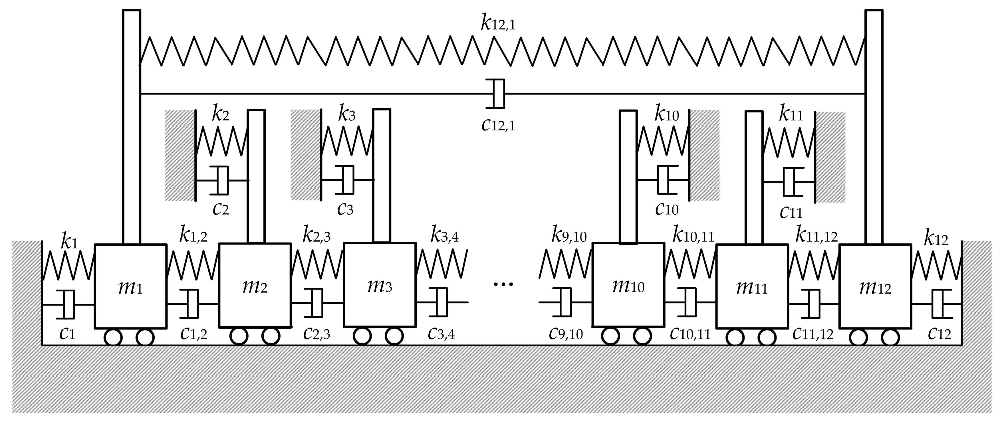
For the actual blade vibration measurement, even if the blade dynamic behavior is fully understood, it is still difficult to eliminate uncertainties in the measurement data [33,34], such as speed fluctuations, system random errors, etc. These uncertainties will affect the evaluation accuracy, therefore, it is better to use simulated data without measurement uncertainties to evaluate the accuracy of the reconstruction methods. A 12-blade assembly simulator was used to evaluate the ICFF performance. The schematic of the simulated model was shown in Figure 3. A mass-spring-damper system represents each blade, which is coupled to its two neighbors through two further spring–damper assemblies. A mathematical model was employed to simulate the forced vibration of the rotating bladed assembly. This mathematical model ignored the effects of the centrifugal force and temperature on the blade stiffness.
The mathematical model of the bladed assembly is given by:
where M, C, K, and F(t) represent the mass matrix, damping matrix, stiffness matrix, and excitation force vector, respectively. Let W(i, j) (1 ≤ i ≤ 12 and 1 ≤ j ≤ 12) represents the element at the ith row and jth column of the matrix W, and above matrixes can be expressed as:
In Equation (14), use 1 for subscripts greater than 12 and 12 for subscripts less than 1. The excitation force fi (t) on blade i is given by:
where Fi is the amplitude of the excitation force, and N represents the count of the blade. N was set to 12 in this paper.
The quality of probe distribution is represented by the probe spacing on the resonance (PSR). The PSR is the ratio of the difference between the times of arrival of a blade at the first and last probe to the period of the blade response at resonance [35], i.e.,:
where ωn represents the natural angular frequency.
Further details on the mathematics of the simulator are given by the literature [36]. According to the literature [37,38], the mistuning coefficient Δfi and the coupling coefficient hi are defined to characterize the degree of blade mistuning and the coupling between blades. The concrete expressions of these two parameters are:
where the subscripts i and j represent the blade number, and k represents the blade nominal stiffness. Let the nominal mass m, stiffness k, and damping c be 1 kg, 8.1 × 10⁵ N/m, and 9 N∙s/m, respectively. Then, the nominal natural frequency of the blade is 900 rad/s according to Equation (18):
Let the distribution of the mistuning coefficients Δfi of the 12-blade assembly simulator conform to a Gaussian distribution with a mean of 0 and a standard deviation of 0.04. The distribution of Δfi is shown in Table 1. Assume that the blade actual mass mi (i = 1, 2, 3… 12) is equal to nominal mass m. The actual natural frequency of the blade was calculated according to Equations (17)–(18) and Table 1, which is shown in Figure 4.
3.2. Simulated Test
The object of the simulated test was to assess analysis techniques for determining the EO and amplitude. Several exhaustive tests were performed using BTT data obtained from the simulator to evaluate the accuracy of the reconstruction method and their sensitivity to various test parameters. These parameters were:
- (1)
- Probe spacing on the resonance (PSR);
- (2)
- The number of revolution (n);
- (3)
- Engine order (EO);
- (4)
- Inter-blade coupling of the mistuned blade (ICoMB);
- (5)
- The number of probes (g);
- (6)
- Noise-to-signal ratio (NSR).
The NSR is defined as the ratio of the r.m.s. value of the noise to the value of the ‘clean’ amplitude of the blade. The NSR was set to 100 points averagely distributed in the range from 0.01 to 0.3. For the same NSR, a white noise generator was used to create 100 distinct noise sequences with which to corrupt the data obtained from the simulator. Each test was repeated using all the white noise sequences for each method on each NSR value. When there is noise in the data, the reconstruction method will contain two types of error [39]:
- (1)
- Bias is where the estimates are incorrect. It is caused by a summated squared noise term in the BTB matrix that does not tend to zero but increases with increasing noise levels. This is an effect of the ICFF model that is used.
- (2)
- Scatter, where there is a range of estimates spread about the mean value, is caused by random variations in the data.
The mean and variance of the recovered EO and amplitude were computed, from which 95 percent confidence intervals were obtained. The best method will exhibit the lowest bias and, preferably, lowest scatter. Six test cases were designed to analyze and compare the performance of the TCFF and ICFF under different test conditions. These are shown in Table 2. Test 1 was specifically chosen to be a very difficult case to analyze. Hence, the other tests were used to investigate whether specific changes in the parameters improve or degrade the performance of the method.
The PSR is a key factor that affects the performance of all BTT algorithms. It is also commonly used to determine the quality of probe distribution for blade synchronous vibration measurement. Currently, there are corresponding methods for optimizing the probe installation layout [40]. Combined with the FEM, the optimization of probe layout can be achieved in actual engineering measurement. Therefore, we set the PSR to a high value (98%) in Test 1. In engineering applications, the probe is inevitably affected by the temperature, airflow, etc., and in severe cases, the measurement data will not be available. In this case, where a limited number of probes were used to measure blade vibration, the failed probe could not participate in the blade vibration analysis, which destroyed the optimization of the probe layout and resulted in a decrease of the PSR. For this reason, the PSR was set to a low value (55 percent) in Test 2.
For TCFF, the blade vibration parameters can be calculated based on the single-revolution data obtained by multiple probes (usually four). However, it is impractical that the single-revolution data are used to identify the blade vibration parameters in engineering applications, considering the effects of system measurement errors. Just as the AR method does [39], it is reasonable to select multi-revolution data, including the blade synchronous resonance region, to determine the true vibration parameters based on the average of the calculation results. For any curve fitting algorithm, such as the single-parameter method, the amount of selected data should include the complete blade resonance response region as much as possible, although there are no specific rules on how many data points should be selected. In the simulated tests, 30 (Test 1) and 50 (Test 3) data points were selected for identifying the vibration parameters to demonstrate the effects of the data amounts on the quality of the identification of each method.
BTT technology is sensitive to a mode with a large amplitude at the blade tip, such as the first-order bending mode. In actual rotating machinery operation, due to mechanical structure or airflow disturbance, the same vibration mode of the blade may be excited at different resonance rotating speeds corresponding to different EO. For BTT algorithms, analysis of the blade vibration at different resonance rotating speeds is essentially a process of reconstructing signals with different degrees of under-sampling. The EO (Test 1: EO = 10; Test 4: EO = 13) was used to analyze and compare the sensitivity of TCFF and ICFF to different degrees of under-sampling, and the EO was also an important parameter for the blade vibration analysis.
Based on the CFF theory, at least three probes are needed to monitor blade synchronous vibration. The least-square method is used to calculate the blade synchronous vibration parameters if more than three probes are used. The TCFF usually uses four probes to increase robustness. However, Tao OuYang used seven probes in the experimental verification of TCFF [31]. So far, there is no optimal choice for the number of probes. Test 5 was designed to verify the performance of TCFF and ICFF on the different number of probes.
Mistuning is a universal feature of the objective existence of the blades, and if inter-blade coupling of the mistuned blade exists, it will affect the performance of the BTT algorithms that only analyze single-frequency signals, such as the single-parameter method, the two-parameter plot method, CFF, and TCFF. The same applies to the ICFF method proposed in this paper. Therefore, Test 6 was specially designed to analyze and compare the sensitivity of TCFF and ICFF to ICoMB.
The noise in the measurement data is difficult to eliminate. The “clean” simulated data was polluted by noise in all simulated tests to make the data closer to the real measurements. The anti-noise performance of each method was verified by using simulated data of different pollution degrees that were represented by the NSR value.
The monitor positions of the probes in Test 1, Test 3, and Test 6 were 0°, 13.1°, 25.3°, and 35.3°. The monitor positions of the probes in Test 4 were 0°, 11.3°, 13.3°, and 25.3°. In Test 2, the monitor positions of the probes were 0°, 6.3°, 10.1°, and 19.8°. In Test 5, the monitor positions of the probes were 0°, 6.3°, 13.1°, 19.1°, 25.3°, 30.2°, and 35.3°. The PSR in Table 2 was calculated according to Equation (16). If the option of the ICoMB is “NO”, it means that the coupling coefficient is set to zero; if it is “Yes”, it means the coupling coefficient is set to nonzero. In this paper, the coupling coefficient hi (i = 1, 2, 3…, 12) was set to 0.1 for the option “Yes”. It is must be stressed that the blade vibration does not influence the adjacent blades when the coupling coefficient is set to zero, even under the condition that the blade is mistuned. For this, it is still a single-frequency vibration for the single blade. However, the synchronous resonance of the single blade will be a superposition of multiple-frequency vibration under the condition that the coupling coefficient is set to nonzero, and it is difficult to distinguish. The coupled vibration of the mistuned blade is a serious challenge for TCFF, since it assumes the blade response is of single-frequency vibration. According to the results shown in Figure 4, the natural frequency of blade 7 is close to that of the adjacent blades. To evaluate the performance of ICFF under the condition of blade mistuning and inter-blade coupling, the simulated data of blade 7 were selected in the simulated tests. The rotating speed was set to accelerate uniformly from 300 to 2400 rpm, which included the resonance rotating speed for all simulated tests. Take the resonance rotating speed as the reference and select half n points before and after the reference point to compose the number of revolutions n. The results of each simulated test were analyzed as follows.
• Test 1:
As expected, Test 1 was a very difficult case. As shown in Figure 5a, the EO identification started to produce biased results at about NSR 0.16 for both methods. For tests with correct EO identification, the 95% confidence intervals of the relative error of the amplitude identification were calculated, which was shown in Figure 5b. The intervals increased with the increase of the NSR for both methods. However, the relative error of amplitude identification of ICFF was lower than that of TCFF.
• Test 2:
Reducing the PSR value to 55 percent produced the most dramatic degrade in the quality of the identification. The correct EO identification did not occur for ICFF before NSR 0.15, and the deviation of EO identification was very large for both methods compared with Test 1. In order to compare the two methods synchronously, Figure 6a only showed that the results of the EO identification in the NSR range of 0.15 and 0.30. The relative error of amplitude identification was calculated after NSR 0.15. The scatter of the relative error was higher than that of Test 1. As already discussed by other literature [35,36,39], curve fits of lower PSR data are generally not conducive to parameter identification.
• Test 3:
Increasing the number of revolutions over which data were used for the identification process can improve the results. The results of EO identification started to be biased when the NSR increase to about 0.18 for both methods, which was shown in Figure 7a. The NSR corresponding to unbiased identification was higher 0.03 than Test 1. However, relative error for amplitude identification increased with increasing the number of data, which was caused by a summated squared noise term in the BTB matrix. This is an effect of the method model that is used. Although the relative error was increased for both methods, the ICFF error increased less than the TCFF.
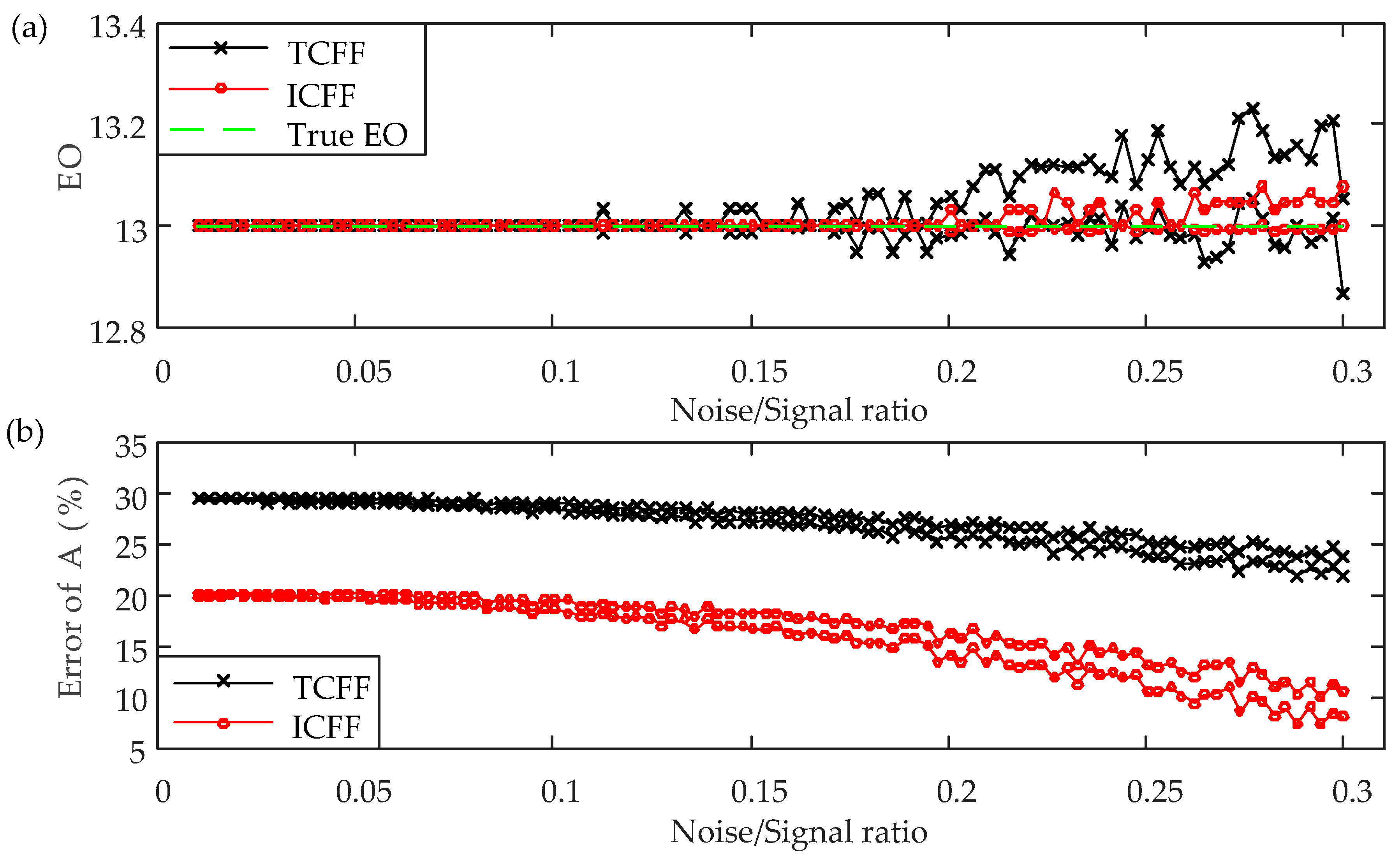
• Test 4:
The results of Test 4 were shown in Figure 8. Increasing the EO of the tip timing data had no visible effect on the accuracy of the EO identification for ICFF. However, the relative error of amplitude identification was higher than that of Test 1. For the same natural frequency, the larger EO, the higher degree of under-sampling. That means the number of samples was less for a period of vibration of the blade. The amplitude that recovered was more sensitive to the number of samples than the EO identification. Although the relative error was increased for both methods, the quality of ICFF was still higher than TCFF.
• Test 5:
Increasing the number of probes made the scatter of EO identification get larger for ICFF, which was shown in Figure 9a. Meanwhile, the relative error of amplitude identification was increased for both methods, which was shown in Figure 9b. The summated squared noise term in the BTB matrix would increase with the number of probes. Then the squared noise term was transferred to amplitude identification. Figure 9b still showed the relative error of ICFF was smaller than TCFF.
• Test 6:
The existence of the ICoMB did not have an effect on the EO identification for both methods, which was shown in Figure 10a. BTT data that consists of two modes corresponding to different EO generally had negative effects on the quality of identification, especially for the reconstruction method that processes the single-frequency signals. However, it did not belong to the range considered in this paper. It needs some future work for processing the multi-frequency signals based on ICFF. The ICoMB made the quality of amplitude identification degrade, which was shown in Figure 10b. However, the relative error of ICFF was still lower than that of TCFF.
3.3. Summary
The percentage of correct EO identification and the mean relative error of amplitude identification were summarized in Table 3 and Table 4 respectively for all simulated tests at the NSR 0.01, 0.05, 0.10, 0.15, 0.20, 0.25 and 0.30.
The results of the EO identification that were less than 80 percent were marked in red in Table 3. Curve fits of lower PSR data are generally not conducive to parameter identification, especially for the EO identification, which was demonstrated by Test 2. Increasing the number of probes would have some negative effect on the EO identification for ICFF, and the degree of influence became significantly larger when the data noise up to 0.20 (Test 5). The higher PSR value and the larger amount of fitted data were conducive to EO identification for both methods. The higher EO value (higher degrees of under-sampling) and coupling between mistuning blades (unconsidering multi-frequency vibration) had little effect on the results of EO identification. Through the comparison from Test 1, Test 3, Test 4 and Test 6, ICFF performance was comparable to TCFF in terms of EO identification.
The relative error for amplitude identification increased with the number of fitted data, which was verified by the results of Test 3. Higher EO value has a more negative effect on the amplitude identification of TCFF than that of ICFF (Test 4). Table 4 showed that the results of amplitude identification of ICFF were more accurate than TCFF, except that the low PSR (Test 2) resulted in the little difference between ICFF and TCFF. The larger number of fitted data and the number of probes would lead to a higher error of amplitude identification for both methods, which was caused by the squared noise term in the BTB matrix that increased with the number of fitted data or probes. Compared with TCFF, ICFF considers the influence of blade vibration on the ToA of the blade tip. This improvement is more consistent with reality and leads to more accuracy of the amplitude identification. This was demonstrated through all of the simulated tests.
Conclusions drawn above were based only on the numerical simulations but not based on the analysis of real signals measured during the experimental tests for a real object under loading conditions. In the experimental tests, different factors may affect the accuracy of the reconstruction method. So, the proposed method will be verified by experimental measurements and analysis in the next section.
4. Method Evaluation Using Experimental Data
The experimental data that was provided by the author of the literature [36] was used to further verify the feasibility of the reconstruction method proposed in this paper. The test rig in the literature [36] was shown in Figure 11a. The radius of the rotor is 60 mm, and there are eight blades. The once per revolution (OPR) sensor was installed near the shaft to provide the rotating speed and a timing reference through detecting a marking on the shaft. Seven optic probes were installed on the casing to measure the blade vibration. The installation angles of the probes were 0° (P0), 18.56° (P1), 36.17° (P2), 53.75° (P3), 72.42° (P4), 119.82° (P5), and 239.06° (P6). The nitrogen shock was used as an exciting force to the rotating blades.
The mode frequency was plotted on the vertical axis in the Campbell diagram of Figure 11b. The diagram plotted the resonant frequency on the vertical axis and the rotating speed on the horizontal axis. The EO lines showed a range from 9 to 15 (blue lines). The seven black dots in the Campbell diagram represent the intersection of the EO lines with the mode frequency. The nominal resonant speeds corresponding to these seven intersections are 7081 rpm (EO = 15), 7613 rpm (EO = 14), 8202rpm (EO = 13), 8907 rpm (EO = 12), 9724 rpm (EO = 11), 10,710 rpm (EO = 10), and 11,890 rpm (EO = 9), respectively.
The displacement of blade 7 measured by probe P0 for rotating speed 6500–12,100 rpm was shown in Figure 12. In the whole speed up, there were seven resonances excited by the nitrogen shock, although the vibration intensity was not completely the same. The EO corresponding to each resonance was predicted through the Campbell diagram (Figure 11b), which was labeled in Figure 12. The similar resonances were also measured by other probes, and here it did not show these vibration waveforms one by one. In the engineering applications, the EO can be predicted through the Campbell diagram, like the experiment in this paper. The EO identification step can be skipped on the condition that the true EO had been known before parameter identification. In this case, the correct EO would be used directly by identification methods to calculate the amplitude, phase, and direct current offset. In this section, the other parameters would be calculated based on the EO that was from prediction rather than identification. Therefore, the reconstruction accuracy was compared for each method base on the EO known.
Although the EO corresponding to each resonance can be predicted through the Campbell diagram, the corresponding amplitude can not be known exactly, which was not the same as the simulated tests where the true signal was obtained in advance. Even if the strain gauges were applied, it also needs a very complex technique for converting the strain to the amplitude of the blade tip, and the strain measurement error as an integrated part of strain data was also transmitted to the amplitude. Therefore, where the true amplitude is unknown, the relative error of reconstruction (REoR) was used to evaluate the quality of reconstruction. If the REoR is greater than zero, the higher REoR, the higher quality of reconstruction for ICFF. In contrast, if the REoR is negative that means the reconstruction accuracy of ICFF is lower than TCFF. The REoR is given by:
where the STDoE represents the standard deviation of reconstruction error for each method, which is indicated by the subscript. The STDoE is given by:
where n represents the number of revolutions, g represents the number of probes, yi,j represents the measurement displacement by probe i at revolution j, and y*i,j represents the reconstruction displacement.
In this experiment, the EO has been determined based on the FEM in advance. So, the true EO can be directly used without identification, which like the CFF does. Based on the results of simulated tests, the more number of probes and fitted data, the higher the reconstruction error for amplitude calculated. Therefore, just four probes (P0, P1, P2, and P3) instead of all were selected to identify the amplitude. For each resonance analysis, the number of fitted data was 20. The reconstruction data of blade 7 measured by probe P0 was plotted in Figure 13. Each resonance was divided by the blue lines. The reconstruction resonance waveforms did not display the whole since only 20 data points were selected for each resonance. The results of reconstruction for measured data by the other probe were similar to Figure 13, which were not shown one by one. It was difficult to determine the quality of the identification only through Figure 13. Therefore, the STDoE and REoR were calculated based on the reconstruction data to achieve the purpose of comparing the quality of the identification. The results of identification for each method were summarized in Table 5.
The REoRs were all greater than zero for all resonance analysis, which was shown in Table 5. That means the reconstruction accuracy of ICFF was higher than that of TCFF. Besides, even for lower PSR like the EO 14 corresponding to PSR 9.03 percent, as long as the true EO is known, the results of amplitude identification still was credible for both methods.
5. Conclusions
In this paper, an improved circumferential Fourier fit method named ICFF was proposed, which considers the blade vibration effect on the TOA. In this method, the ToA is not only dependent on the rotating speed and monitoring position, but also on blade vibration. Compared with TCFF, this improvement is more consistent with reality. A 12-blade assembly simulator and experimental data were used to evaluate the ICFF performance. The simulated results showed that the ICFF performance is comparable to TCFF in terms of EO identification, except the lower PSR or more number probes have a more negative effect on ICFF, which results in the poor performance of ICFF in Test 2 and Test 5. However, the accuracy of amplitude identification is higher for ICFF than TCFF on all test conditions. Meanwhile, the higher accuracy of the reconstruction of ICFF was further verified by experimental data, where the quality of reconstruction was higher for ICFF than TCFF in all measurement resonance analysis. The propagation of uncertainty in measurements, the method of sensor layout determination, and the BTT data analysis that consists of two or more modes corresponding to different EOs will be the focus of further research work.
Author Contributions
Conceptualization, Z.L. and F.D.; methodology, Z.L.; validation, F.D.; investigation, Z.L. and G.N.; writing—original draft preparation, Z.L.; writing—review and editing, L.M.; visualization, J.J. and X.F.; funding acquisition, F.D. All authors have read and agreed to the published version of the manuscript.
Funding
This research was funded by Equipment Pre-research Field Fund (Grant Nos. 61400040303 and 61405180505), National Science and Technology Major Project (Grant No. 2017-V-0009), National Natural Science Foundations of China (Grant Nos. 51775377, 61971307 and 61905175), National Key Research and Development Plan (Grant No. 2017YFF0204800), Natural Science Foundations of Tianjin City (Grant No. 17JCQNJC01100), Science and Technology on Underwater Information and Control Laboratory (Grant No. 6142218081811), and 2019 Guangdong Provincial Market Supervision Administration Quality and Safety Supervision Scientific Research Project (Grant No. 2019ZZ02).
Conflicts of Interest
The authors declare no conflict of interest.
Nomenclature
| A | the amplitude of blade vibration | N | number of blades |
| B | coefficient matrix | R | distance from the blade tip to the center of the rotor |
| c | nominal damping of the blade | ||
| ci | damping of blade i (i = 1, 2, 3…) | REoR | the relative error of reconstruction |
| C | damping matrix | STDoE | the standard deviation of reconstruction error |
| ci,j | coupling damping | ||
| d | the direct current offset | Sk | fitted residual |
| fi(t) | excitation force | equivalent fitted residual | |
| Δfi | mistuning coefficient | t | time of arrival (ToA) |
| F(t) | excitation force vector | ω | angular vibration frequency |
| Fi | the amplitude of the excitation force | ωn | angular natural frequency |
| ωv | angular rotating speed | ||
| g | number of the probe | average angular rotating speed | |
| hi | coupling coefficient | X | parameter matrix |
| k | nominal stiffness of the blade | y | vibration displacement of the blade |
| ki | stiffness of blade i (i = 1, 2, 3…) | Y | displacement vector |
| K | stiffness matrix | β | installed position of the probe |
| ki,j | coupling stiffness | equivalent monitoring position | |
| m | the nominal mass of the blade | ε | the angle of the blade from the first probe when the mark passes the OPR sensor |
| mi | mass of blade i (i = 1, 2, 3…) | ||
| M | mass matrix | ||
| n | number of revolution | ϕ | vibration phase |
References
- Kumar, S.; Roy, N.; Ganguli, R. Monitoring Low Cycle Fatigue Damage in Turbine Blade Using Vibration Characteristics. Mech. Syst. Signal. Process. 2007, 21, 480–501. [Google Scholar] [CrossRef]
- Madhavan, S.; Jain, R.; Sujatha, C.; Sekhar, A.S. Vibration Based Damage Detection of Rotor Blades in a Gas Turbine Engine. Eng. Fail. Anal. 2014, 46, 26–39. [Google Scholar] [CrossRef]
- Till, H.; Stefan, B. Axial Fan Blade Vibration Assessment under Inlet Cross-Flow Conditions Using Laser Scanning Vibrometry. Appl. Sci. 2017, 7, 862. [Google Scholar] [CrossRef] [Green Version]
- Presas, A.; Valentin, D.; Valero, C.; Egusquiza Montagut, M.; Egusquiza, E. Experimental Measurements of the Natural Frequencies and Mode Shapes of Rotating Disk-Blades-Disk Assemblies from the Stationary Frame. Appl. Sci. 2019, 9, 3864. [Google Scholar] [CrossRef] [Green Version]
- Battiato, G.; Firrone, C.M.; Berruti, T.M. Forced Response of Rotating Bladed Disks: Blade Tip-Timing Measurements. Mech. Syst. Signal. Process. 2017, 85, 912–926. [Google Scholar] [CrossRef]
- Beauseroy, P.; Lengellé, R. Nonintrusive Turbomachine Blade Vibration Measurement System. Mech. Syst. Signal. Process. 2007, 21, 1717–1738. [Google Scholar] [CrossRef]
- Russhard, P. Development of a Blade Tip Timing Based Engine Health Monitoring System. PhD. Thesis, The University of Manchester, Manchester, UK, 2010. [Google Scholar]
- Ye, D.; Duan, F.; Jiang, J.; Cheng, Z.; Niu, G.; Shan, P.; Zhang, J. Synchronous Vibration Measurements for Shrouded Blades Based on Fiber Optical Sensors with Lenses in a Steam Turbine. Sensors 2019, 19, 2501. [Google Scholar] [CrossRef] [Green Version]
- Ye, D.; Duan, F.; Jiang, J.; Niu, G.; Liu, Z.; Li, F. Identification of Vibration Events in Rotating Blades Using a Fiber Optical Tip Timing Sensor. Sensors 2019, 19, 1482. [Google Scholar] [CrossRef] [PubMed] [Green Version]
- Russhard, P. The Rise and Fall of the Rotor Blade Strain Gauge. In Mechanisms and Machine Science; Springer: Cham, Switzerland, 2015; pp. 27–37. [Google Scholar] [CrossRef]
- Heath, S.; Imregun, M. A Survey of Blade Tip-Timing Measurement Techniques for Turbomachinery Vibration. J. Eng. Gas. Turbines Power 1998, 120, 784. [Google Scholar] [CrossRef]
- Schoenenborn, H.; Breuer, T. Aeroelasticity at Reversed Flow Conditions—Part Ⅱ: Application to Compressor Surge. J. Turbomach. 2011, 134, 061031–061035. [Google Scholar] [CrossRef]
- Rzadkowski, R.; Rokicki, E.; Piechowski, L.; Szczepanik, R. Analysis of Middle Bearing Failure in Rotor Jet Engine Using Tip-Timing and Tip-Clearance Techniques. In Proceedings of the ASME Turbo Expo 2014, Dusseldorf, Germany, 16–20 June 2014. [Google Scholar]
- Krause, C.; Giersch, T.; Stelldinger, M.; Hanschke, B.; Kühhorn, A. Asynchronous Response Analysis of Non-Contact Vibration Measurements on Compressor Rotor Blades. In Proceedings of the ASME Turbo Expo 2017: Turbomachinery Technical Conference and Exposition, Charlotte, NC, USA, 26–30 June 2017. [Google Scholar]
- Wang, W.; Ren, S.; Chen, L.; Huang, S. Investigation on the Method of Blade Synchronous Vibration Parameter Identification (Simulation). J. Vib. Shock 2017, 36, 120–126. [Google Scholar] [CrossRef]
- Wang, W.; Ren, S.; Chen, L.; Shao, H. Test for Synchronous Vibration Parametric Identification Method of a Turbine’s Blades. J. Vib. Shock 2017, 36, 127–133. [Google Scholar] [CrossRef]
- Watkins, W.; Robinson, W.; Chi, R. Noncontact Engine Blade Vibration Measurements and Analysis. In Proceedings of the AIAA/SAE/ASME/ASEE 21st Joint Propulsion Conference, Monterey, CA, USA, 8–10 July 1985. [Google Scholar]
- Zhang, Y.; Duan, F.; Fang, Z.; Ou, Y.; Ye, S. Analysis of Non-Contact Asynchronous Vibration of Rotating Blades Based on Tip-Timing. Chin. J. Mech. Eng. 2008, 44, 147–150. [Google Scholar] [CrossRef]
- Vercoutter, A.; Lardies, J.; Berthillier, M.; Talon, A.; Burgardt, B. Improvement of Compressor Blade Vibrations Spectral Analysis from Tip Timing Data: Aliasing Reduction. In Proceedings of the ASME Turbo Expo 2013: Turbine Technical Conference and Exposition, San Antonio, TX, USA, 7–8 June 2013. [Google Scholar]
- Kharyton, V.; Bladh, R. Using Tiptiming and Strain Gauge Data for the Estimation of Consumed Life in a Compressor Blisk Subjected to Stall-Induced Loading. In Proceedings of the ASME Turbo expo 2014: Turbine Technical Conference and Exposition, Duesseldorf, Germany, 16–20 June 2014. [Google Scholar]
- Kharyton, V.; Dimitriadis, G.; Defise, C. A Discussion on the Advancement of Blade Tip Timing Data Processing. In Proceedings of the ASME Turbo Expo 2017: Turbomachinery Technical Conference and Exposition, Charlotte, NC, USA, 26–30 June 2017. [Google Scholar]
- Lin, J.; Hu, Z.; Chen, Z.-S.; Yang, Y.-M.; Xu, H.-L. Sparse Reconstruction of Blade Tip-Timing Signals for Multi-Mode Blade Vibration Monitoring. Mech. Syst. Signal. Process. 2016, 81, 250–258. [Google Scholar] [CrossRef]
- Ewins, D.J. Modal Analysis for Rotating Machinery. In Modal Analysis and Testing; Springer: New York, NY, USA, 1999; pp. 549–568. [Google Scholar]
- Zablotskiy, I.Y.; Korostelev, Y.A. Measurement of Resonance Vibrations of Turbine Blades with the Elura Device; Foreign Technology Div Wright-Patterson AFB OH: Dayton, OH, USA, 1978. [Google Scholar]
- Heath, S. A New Technique for Identifying Synchronous Resonances Using Tip-Timing. J. Eng. Gas. Turbines Power 2000, 122, 219–225. [Google Scholar] [CrossRef]
- Gallego-Garrido, J.; Dimitriadis, G.; Wright, J.R. A Class of Methods for the Analysis of Blade Tip Timing Data from Bladed Assemblies Undergoing Simultaneous Resonances—Part I: Theoretical Development. Int. J. Rotat. Mach. 2007, 2007. [Google Scholar] [CrossRef]
- Gallego-Garrido, J.; Dimitriadis, G.; Carrington, I.B.; Wright, J.R. A Class of Methods for the Analysis of Blade Tip Timing Data from Bladed Assemblies Undergoing Simultaneous Resonances—Part Ⅱ: Experimental Validation. Int. J. Rotat. Mach. 2007, 2007. [Google Scholar] [CrossRef]
- Joung, K.-K.; Kang, S.-C.; Paeng, K.-S.; Park, N.-G.; Choi, H.-J.; You, Y.-J.; Von Flotow, A. Analysis of Vibration of the Turbine Blades Using Non-Intrusive Stress Measurement System. In Proceedings of the PWR2006, Atlanta, GA, USA, 2–4 May 2006. [Google Scholar]
- Guo, H.; Duan, F.; Zhang, J. Blade Resonance Parameter Identification Based on Tip-Timing Method without the Once-Per Revolution Sensor. Mech. Syst. Signal. Process. 2016, 66, 625–639. [Google Scholar] [CrossRef]
- Chen, K.; Wang, W.; Zhang, X.; Zhang, Y. New Step to Improve the Accuracy of Blade Tip Timing Method without Once Per Revolution. Mech. Syst. Signal. Process. 2019, 134, 106321. [Google Scholar] [CrossRef]
- Ou, Y.; Duan, F.; Li, M.; Kong, X. Method for Identifying Rotating Blade Synchronous Vibration at Constant Speed. J. Tianjin Univ. 2011, 44, 742–746. [Google Scholar] [CrossRef]
- Heath, S.; Imregun, M. An Improved Single-Parameter Tip-Timing Method for Turbomachinery Blade Vibration Measurements Using Optical Laser Probes. Int. J. Mech. Sci. 1996, 38, 1047–1058. [Google Scholar] [CrossRef]
- Rossi, G.; Brouckaert, J.-F. Design of Blade Tip Timing Measurement Systems Based on Uncertainty Analysis. In Proceedings of the International Instrumentation Symposium, San Diego, CA, USA, 4–8 June 2012. [Google Scholar]
- Russhard, P. Blade Tip Timing (BTT) Uncertainties. In Proceedings of the 12th International A.I.VE.LA. Conference on Vibration Measurements by Laser and Noncontact Techniques, Anona, Italy, 29 June–1 July 2016. [Google Scholar]
- Dimitriadis, G.; Carrington, I.B.; Wright, J.R.; Cooper, J.E. Blade-Tip Timing Measurement of Synchronous Vibrations of Rotating Bladed Assemblies. Mech. Syst. Signal. Process. 2002, 16, 599–622. [Google Scholar] [CrossRef]
- Ou, Y. Rotating Blade Vibration Detection and Parameters Identification Technique Using Blade Tip-Timing. PhD. Thesis, Tianjin University, Tianjin, China, 2011. [Google Scholar]
- Wei, S.T.; Pierre, C. Localization Phenomena in Mistuned Assemblies with Cyclic Symmetry Part I: Free Vibrations. J. Vib. Acoust. Stress Reliab. Des. 1988, 110, 429–438. [Google Scholar] [CrossRef]
- Wei, S.T.; Pierre, C. Localization Phenomena in Mistuned Assemblies with Cyclic Symmetry Part Ⅱ: Forced Vibrations. J. Vib. Acoust. Stress Reliab. Des. 1988, 110, 439–449. [Google Scholar] [CrossRef]
- Carrington, I.B.; Wright, J.R.; Cooper, J.E.; Dimiadis, G. A Comparison of Blade Tip Timing Data Analysis Methods. Proc. Inst. Mech. Eng. Part G J. Aerosp. Eng. 2001, 215, 301–312. [Google Scholar] [CrossRef]
- Diamond, D.H.; Stephan Heyns, P. A Novel Method for the Design of Proximity Sensor Configuration for Rotor Blade Tip Timing. J. Vib. Acoust. 2018, 140. [Google Scholar] [CrossRef]
Figure 1.
(a) Under-sampling of asynchronous vibration and (b) under-sampling of synchronous vibration.
Figure 1.
(a) Under-sampling of asynchronous vibration and (b) under-sampling of synchronous vibration.

Figure 2.
The schematic of the blade tip timing (BTT) measurement. The once per revolution (OPR) sensor monitors the rotating speed through the mark on the shaft and provides a timing reference for the BTT measurement system. The probe is responsible for monitoring the ToA. R represents the distance from the blade tip to the center of the rotor, and y/R represents the circumferential angle of the blade vibration. β represents the monitoring position, and ε represents the angle of the blade from the first probe when the mark passes the OPR sensor.

Figure 3.
The simulated model. mi, ki, and ci (i = 1, 2, 3... 12) represent the mass, stiffness, and damping coefficient of blade i, respectively. ki, j and ci, j (|i − j| = 1) represent the coupling stiffness and coupling damping coefficient between adjacent blades.
Figure 3.
The simulated model. mi, ki, and ci (i = 1, 2, 3... 12) represent the mass, stiffness, and damping coefficient of blade i, respectively. ki, j and ci, j (|i − j| = 1) represent the coupling stiffness and coupling damping coefficient between adjacent blades.

Figure 4.
The mistuning frequency of the blade.

Figure 5.
Results of Test 1. (a) 95% confidence intervals of the engine order (EO) identification and (b) 95% confidence intervals of the relative error of the amplitude identification.
Figure 5.
Results of Test 1. (a) 95% confidence intervals of the engine order (EO) identification and (b) 95% confidence intervals of the relative error of the amplitude identification.

Figure 6.
Results of Test 2. (a) 95% confidence intervals of the EO identification and (b) 95% confidence intervals of the relative error of the amplitude identification.
Figure 6.
Results of Test 2. (a) 95% confidence intervals of the EO identification and (b) 95% confidence intervals of the relative error of the amplitude identification.

Figure 7.
Results of Test 3. (a) 95% confidence intervals of the EO identification and (b) 95% confidence intervals of the relative error of the amplitude identification.
Figure 7.
Results of Test 3. (a) 95% confidence intervals of the EO identification and (b) 95% confidence intervals of the relative error of the amplitude identification.

Figure 8.
Results of Test 4. (a) 95% confidence intervals of the EO identification and (b) 95% confidence intervals of the relative error of the amplitude identification.
Figure 8.
Results of Test 4. (a) 95% confidence intervals of the EO identification and (b) 95% confidence intervals of the relative error of the amplitude identification.

Figure 9.
Results of Test 5. (a) 95% confidence intervals of the EO identification and (b) 95% confidence intervals of the relative error of the amplitude identification.
Figure 9.
Results of Test 5. (a) 95% confidence intervals of the EO identification and (b) 95% confidence intervals of the relative error of the amplitude identification.

Figure 10.
Results of Test 6. (a) 95% confidence intervals of the EO identification and (b) 95% confidence intervals of the relative error of the amplitude identification.
Figure 10.
Results of Test 6. (a) 95% confidence intervals of the EO identification and (b) 95% confidence intervals of the relative error of the amplitude identification.

Figure 11.
(a) The test rig and (b) the blade Campbell diagram.

Figure 12.
The displacement of blade 7 measured by probe P0.

Figure 13.
The reconstruction data of blade 7 measured by probe P0.


Table 1.
The distribution of the mistuning coefficient Δfi (%).
| Δf1 | Δf2 | Δf3 | Δf4 | Δf5 | Δf6 | Δf7 | Δf8 | Δf9 | Δf10 | Δf11 | Δf12 |
|---|---|---|---|---|---|---|---|---|---|---|---|
| −0.706 | 3.165 | −5.328 | −9.319 | −5.796 | 1.334 | 1.565 | 1.806 | −0.521 | 0.734 | −1.904 | 3.448 |
Table 2.
The simulated test.
| Test | PSR | n | True EO | g | ICoMB |
|---|---|---|---|---|---|
| Test 1 | 98% | 30 | 10 | 4 | No |
| Test 2 | 55% | 30 | 10 | 4 | No |
| Test 3 | 98% | 50 | 10 | 4 | No |
| Test 4 | 98% | 30 | 13 | 4 | No |
| Test 5 | 98% | 30 | 10 | 7 | No |
| Test 6 | 98% | 30 | 10 | 4 | Yes |
The parameters whose background was shaded were the changed parameters relative to Test 1.
Table 3.
Percentage of correct EO identification following the noise-to-signal ratio (NSR) values.
| NSR | Test 1 | Test 2 | Test 3 | Test 4 | Test 5 | Test 6 | ||||||
|---|---|---|---|---|---|---|---|---|---|---|---|---|
| TCFF | ICFF | TCFF | ICFF | TCFF | ICFF | TCFF | ICFF | TCFF | ICFF | TCFF | ICFF | |
| 0.01 | 100% | 100% | 0 | 0 | 100% | 100% | 100% | 100% | 100% | 100% | 100% | 100% |
| 0.05 | 100% | 100% | 1% | 0 | 100% | 100% | 100% | 100% | 100% | 100% | 100% | 100% |
| 0.10 | 100% | 100% | 14% | 0 | 100% | 100% | 100% | 100% | 100% | 91% | 100% | 100% |
| 0.15 | 100% | 100% | 19% | 2% | 100% | 100% | 99% | 100% | 100% | 87% | 100% | 100% |
| 0.20 | 98% | 97% | 29% | 5% | 100% | 100% | 96% | 99% | 98% | 66% | 98% | 100% |
| 0.25 | 96% | 98% | 12% | 15% | 98% | 99% | 88% | 100% | 92% | 46% | 96% | 99% |
| 0.30 | 88% | 88% | 18% | 11% | 96% | 96% | 78% | 96% | 89% | 55% | 87% | 94% |
The results of the EO identification that were less than 80 percent were marked in red.
Table 4.
Mean relative error of the amplitude identification following NSR values.
| NSR | Test 1 | Test 2 | Test 3 | Test 4 | Test 5 | Test 6 | ||||||
|---|---|---|---|---|---|---|---|---|---|---|---|---|
| TCFF | ICFF | TCFF | ICFF | TCFF | ICFF | TCFF | ICFF | TCFF | ICFF | TCFF | ICFF | |
| 0.01 | 13.49% | 4.06% | — | — | 28.74% | 23.82% | 29.41% | 20.04% | 15.97% | 14.53% | 18.29% | 10.32% |
| 0.05 | 13.42% | 4.00% | — | — | 28.59% | 23.64% | 29.29% | 19.96% | 15.87% | 14.46% | 18.19% | 10.19% |
| 0.10 | 13.03% | 3.56% | — | — | 28.29% | 23.37% | 28.70% | 18.97% | 15.59% | 14.25% | 17.97% | 10.02% |
| 0.15 | 12.69% | 3.35% | 18.63% | 19.07% | 27.63% | 22.48% | 27.62% | 17.53% | 15.72% | 14.47% | 17.38% | 9.30% |
| 0.20 | 12.23% | 2.98% | 19.10% | 19.38% | 26.83% | 21.63% | 26.39% | 15.25% | 15.24% | 14.16% | 16.58% | 8.47% |
| 0.25 | 11.30% | 1.92% | 18.30% | 19.50% | 26.22% | 20.94% | 24.54% | 11.78% | 15.78% | 14.92% | 15.56% | 7.65% |
| 0.30 | 10.54% | 1.23% | 17.32% | 18.29% | 24.73% | 19.32% | 22.72% | 9.24% | 14.35% | 13.70% | 15.19% | 7.17% |
The results of amplitude identification that were higher than 20 percent were marked in red.
Table 5.
The results of the identification.
| Resonance | PSR | EO | Identification | REoR | |||||
|---|---|---|---|---|---|---|---|---|---|
| Amplitude (μm) | Direct Current Offset (μm) | STDoE (μm) | |||||||
| TCFF | ICFF | TCFF | ICFF | TCFF | ICFF | ||||
| 1 | 23.96% | 15 | 63.01 | 43.01 | 4.84 | 3.83 | 11.51 | 9.69 | +15.81% |
| 2 | 9.03% | 14 | 78.48 | 67.59 | 7.32 | 8.67 | 27.11 | 23.85 | +12.02% |
| 3 | 94.10% | 13 | 83.55 | 71.19 | 13.50 | 12.70 | 18.48 | 16.72 | +9.52% |
| 4 | 79.17% | 12 | 99.28 | 85.26 | 2.29 | 2.23 | 31.61 | 29.02 | +8.16% |
| 5 | 64.24% | 11 | 88.47 | 75.75 | 3.38 | 3.77 | 16.20 | 14.99 | +7.47% |
| 6 | 49.31% | 10 | 127.63 | 107.87 | 2.36 | 1.73 | 28.16 | 24.05 | +14.57% |
| 7 | 34.38% | 9 | 84.92 | 75.03 | 4.69 | 3.77 | 10.31 | 9.28 | +9.99% |
© 2020 by the authors. Licensee MDPI, Basel, Switzerland. This article is an open access article distributed under the terms and conditions of the Creative Commons Attribution (CC BY) license (http://creativecommons.org/licenses/by/4.0/).
Share and Cite
MDPI and ACS Style
Liu, Z.; Duan, F.; Niu, G.; Ma, L.; Jiang, J.; Fu, X. An Improved Circumferential Fourier Fit (CFF) Method for Blade Tip Timing Measurements. Appl. Sci. 2020, 10, 3675. https://doi.org/10.3390/app10113675
AMA Style
Liu Z, Duan F, Niu G, Ma L, Jiang J, Fu X. An Improved Circumferential Fourier Fit (CFF) Method for Blade Tip Timing Measurements. Applied Sciences. 2020; 10(11):3675. https://doi.org/10.3390/app10113675
Chicago/Turabian StyleLiu, Zhibo, Fajie Duan, Guangyue Niu, Ling Ma, Jiajia Jiang, and Xiao Fu. 2020. "An Improved Circumferential Fourier Fit (CFF) Method for Blade Tip Timing Measurements" Applied Sciences 10, no. 11: 3675. https://doi.org/10.3390/app10113675
Note that from the first issue of 2016, this journal uses article numbers instead of page numbers. See further details here.