Genetic Algorithm with Radial Basis Mapping Network for the Electricity Consumption Modeling

Abstract

The modified backpropagation algorithm based on the backpropagation with momentum is used for the parameters updating of a radial basis mapping (RBM) network, where it requires of the best hyper-parameters for more precise modeling. Seeking of the best hyper-parameters in a model it is not an easy task. In this article, a genetic algorithm is used to seek of the best hyper-parameters in the modified backpropagation for the parameters updating of a RBM network, and this RBM network is used for more precise electricity consumption modeling in a city. The suggested approach is called genetic algorithm with a RBM network. Additionally, since the genetic algorithm with a RBM network starts from the modified backpropagation, we compare both approaches for the electricity consumption modeling in a city.

1. Introduction

Across the world, populations in cities have been growing. To avoid overcrowding and the accompanying decrease in quality of life, it is essential to introduce some research. To improve the efficiency, the electricity consumption of the city may use the modeling as one alternative to conduct the data analysis for understanding its behavior. Then, the investigation of approaches that allow the electricity consumption modeling becomes transcendent. The modeling of events requires a meticulous study of past events and the relationships between them, and from there, it tries to extrapolate a present event.

The modeling has many applications, such as prediction [1,2,3,4], pattern recognition [5,6,7,8], detection [9,10,11], and classification [12,13,14]. The backpropagation is a supervised algorithm was used in a radial basis mapping (RBM) network for the modeling; the value of the scale parameters was adjusted according to a cost [15,16,17].

Later, one modified backpropagation algorithm based on the backpropagation with momentum [18,19,20,21] was used for the parameter updating of a RBM network; it requires the best hyper-parameters for a more precise modeling. Seeking of the best hyper-parameters in a model it is not an easy task. There are plenty of options to evaluate it; grid search or random search are common practices, but these algorithms present the disadvantage that the user has to pick the correct options. Hence, we use a genetic algorithm as the best alternative to seek these values.

Genetic algorithms are frequently used for the modeling. The optimization with genetic algorithms is studied in [22,23,24,25]. In [26,27,28,29], the genetic algorithm for path planning is discussed. The fuzzy systems with genetic algorithms are addressed in [30,31,32,33]. In [34,35,36,37], the neural networks with genetic algorithms are introduced. Since the genetic algorithms are highly utilized in the modeling, it is attractive to use a genetic algorithm to seek the best hyper-parameters for more precise modeling.

In this article, a genetic algorithm is used to seek the best hyper-parameters in the modified backpropagation for the parameters updating of a RBM network, and this RBM network is used for more precise electricity consumption modeling in a city. The suggested approach is called genetic algorithm with a RBM network. The approach was developed based on the next steps:

(1)

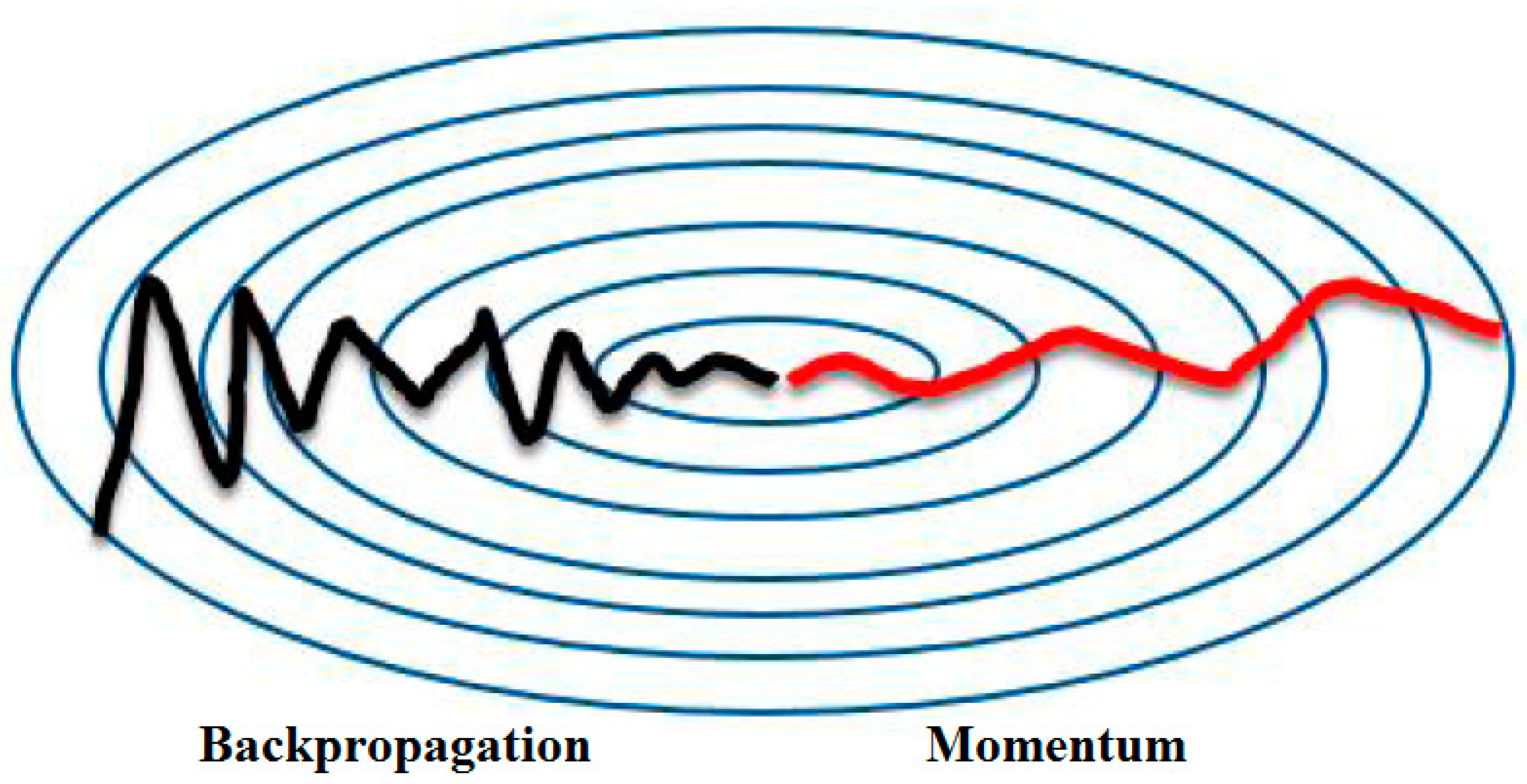
The modified backpropagation. We use the momentum to update the parameters’ velocities. The momentum encourages the movements in the correct direction, with the advantage of a velocity increasing in the convergence. Using the momentum, the trajectory has a smooth behavior. We use the modified backpropagation for the modeling.

(2)

The genetic algorithm. The genetic algorithm is a strategy of searching based on the natural selection and genetic laws. It combines the survival principle of the best solutions for an issue; with the interchange of random information, it forms a searching algorithm capable of exploring the promising areas of historic information in the solutions set. We seek the hyper-parameters to be updated for a more precise modeling.

(3)

The combination of the genetic algorithm with modified backpropagation is called the genetic algorithm with a RBM network for more precise modeling. First, we seek the hyper parameters and find their best values by the genetic algorithm. Second, we use the modified backpropagation with the best hyper-parameters for the modeling.

Finally, since the suggested approach called genetic algorithm with an RBM network starts from the modified backpropagation, we compare both approaches for the electricity consumption modeling in a city.

The remainder of this article is organized in as follows. Section 2 presents the RBM network and the modified backpropagation. The genetic algorithm with an RBM network is explained in Section 3. Section 4 shows the comparison results of the genetic algorithm with the RBM network and modified backpropagation for the electricity consumption modeling in a city. Conclusions and future steps are detailed in Section 5.

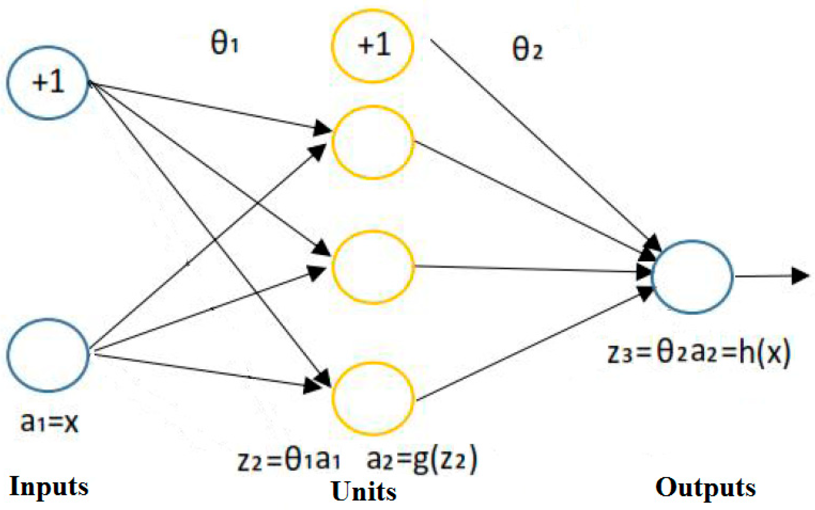
2. The RBM Network Modeling

The form to update the parameters of the RBM network is that each unit assigns information to the next unit and it receives information from the past unit. We need the training for the successful modeling in a RBM network. The training is developed from one epoch to other epoch until the parameters reach constant values and the error converges to the minimum value. In addition, we need that the training data are updated in a random form.

In the training stage, the RBM network updates the modeling of its outputs each time, we find a result, and we compare these outputs with targets; in this way the RBM network decreases its error. The parameters take random initial values, and these parameters are updated through the time.

We use other testing data to evaluate the precision in the RBM network. It consists of taking $80\%$ of data for the training and taking $20\%$ of data for the testing. The first stage is the training where the parameters are updated. Additionally, after of the training, the second stage is the testing where the parameters remain constant.

In the modeling, the training and the testing stages are transcendent. We need successful performance of both stages for a precise modeling.

The RBM network is seen in Figure 1.

We define the RBM network as:

$$\begin{array}{c}{a}_1=x\\ z_2={\theta }_1{a}_1\\ a_2=g(z_2)\\ z_3=h(x)={\theta }_2{a}_2\end{array}$$

(1)

with $a_1$ as the input, $a_2=g(z_2)$ as the unit output, and $z_3=h(x)$ as the output.

We describe the units by Gaussian mappings as:

$$g(z_2)=\frac{1}{\sigma \sqrt{2\pi }}{e}^{-\frac{{(z_2-c)}^2}{2{\sigma }^2}}$$

(2)

with $z_2$ as the input of the Gaussian mapping, $c$ as the center of the Gaussian mapping, and $\sigma$ as the width of the Gaussian mapping.

For the training of the RBM network via the backpropagation we use the next procedure:

(1)

We initialize the parameters with random values.

(2)

We implement the forward propagation of $h(x)$.

(3)

We find the cost $J({\theta }_1,{\theta }_2)$.

(4)

We implement the backpropagation.

(5)

We utilize the backpropagation to update the parameters $({\theta }_1,{\theta }_2)$.

The strategies for the updating of the RBM network that we describe in the next sub-sections have the characteristic of taking into account much data.

Modified Backpropagation

It is possible to make more precise the convergence of the backpropagation by using the momentum [18,19,20,21]. The goals of the momentum are to increase the movements in the correct direction, and to decrease the movements in the incorrect directions. The momentum takes into account the past backpropagation to smooth the updating.

Instead, to use the backpropagation to update the parameters’ vectors, we use the momentum to update the parameters’ velocities. The momentum encourages the movements in the correct direction, with the advantage of the velocity increasing for the convergence. Using the momentum, the trajectory has smooth behavior (please see Figure 2).

Applying the momentum to the backpropagation, the parameter updating is:

$$\begin{array}{c}{V}_{d\theta 1}=\beta V_{d\theta 1}+\left(1-\beta \right)\hspace{0.17em}\left\{\left[(z_3-y){\theta }_2\left(\frac{\frac{c-z_2}{{\sigma }^2}{e}^{-\frac{{(z_2-c)}^2}{2{\sigma }^2}}}{\sigma \sqrt{2\pi }}\right)\right]\hspace{0.17em}{a}_1\right\}\\ {\theta }_1={\theta }_1-\alpha V_{d\theta 1}\end{array}$$

(3)

$$\begin{array}{c}{V}_{d\theta 2}=\beta V_{d\theta 2}+\left(1-\beta \right)(z_3-y)a_2\\ {\theta }_2={\theta }_2-\alpha V_{d\theta 2}\end{array}$$

(4)

with $\beta$ as a momentum constant with a value between $0$ and $1$, and $\alpha$ as the modeling factor with a value between $0$ and $1$.

We express the algorithm of the modified backpropagation as:

(1)

For epochs $e=1,\hspace{0.17em}2,\dots ,\hspace{0.17em}n$.

(2)

We update the backpropagation for each epoch with Equations (3) and (4).

(3)

We repeat it for each epoch.

3. Genetic Algorithm with RBM Network

The goal of the RBM network is to minimize its error for the behavioral modeling. The training depends of some parameters called hyper-parameters; the improved algorithm is a consequence of choosing the hyper-parameters. We seek the hyper-parameters which led the RBM network to reach more precise modeling results.

In this article, we seek the hyper-parameters in the genetic algorithm to reach a more precise modeling result as:

• $\sigma$—width of the Gaussian mapping.
• $\beta$—momentum constant.

Remark 1.

Another additional parameter could be sought in the genetic algorithm to reach a more precise modeling result—$\alpha$. But the consideration of this third parameter with the other two hyper-parameters could increase the computational cost. Hence, two hyper-parameters are sought in this article.

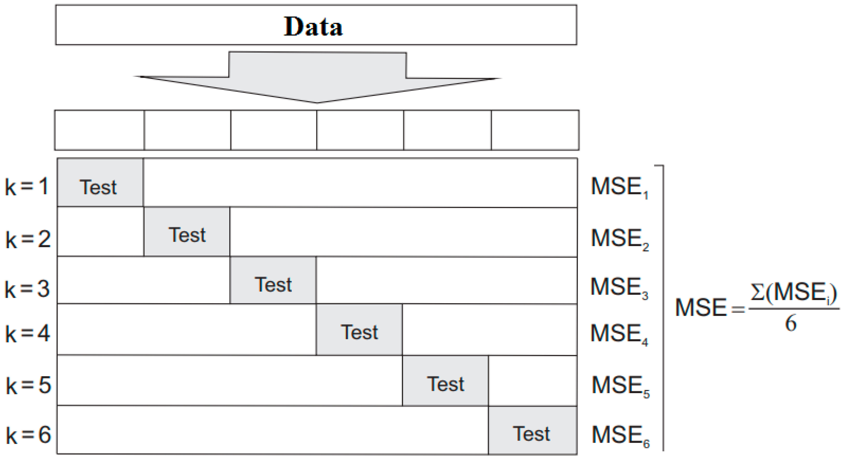
3.1. K-Fold Cross-Validation

To find the hyper-parameters, i.e., the parameters for a more precise modeling, the most used strategy is the k-fold cross-validation.

The system of the k-fold cross-validation supposes $k$ operations, in which the training algorithm utilizes $k-1$ subsets to train, and it lets out one of them. The out subset is rotated at each iteration such as at the final of operations, all the data form part of the training and testing in one moment ($k-1$ time to train and $1$ to test). The measure of the error is the arithmetic mean of errors in different iterations; one example can be seen in Figure 3 for $k=6$.

The k-fold cross-validation is the strategy to substitute the mathematical expectation with an average of the validation set.

3.2. Genetic Algorithm

The genetic algorithm is a strategy of searching based on the combination of the survival principle of the best solutions for an issue, and the interchange of random information. This searching algorithm is capable of exploring the promising areas in the historic information of solutions.

The genetic algorithm is highly trusted. The multiple degrees of liberty let it adapt the searching to the necessities of each issue. To solve a particular issue, we must put much care to its implementation, with the next steps:

• We must use chromosomes to find a solution. A chromosome is just a fancy word to talk about a solution codified as a sequence of bits. Each chromosome is codified in a bits representation.
• The creation of the initial population. It can be generated randomly or through the use of a heuristic technique, such that the chromosomes of the first generation are reasonably well placed in the search set. With a good initialization you can save computational cost and time.
• The evaluation mapping. It requires the knowledge of the issue that is being addressed to assign a degree of aptitude to the different chromosomes, such that, after evaluation, the genetic algorithm can find the best chromosomes in the population.
• The reproduction. The objective of the reproduction system is to find a new population from the current population. Its implementation requires the creation of a chromosomal subset of the current population that is reproduced to generate the new population, a subset that is called fathers. Once the set of fathers is formed, their reproduction is done by applying the genetic operators of crossing to randomly found chromosomes of this set until completing a new generation.
• The natural selection. The most suitable chromosomes of the current population are evaluated by selection per tournament to pass to the next generation.
• The criterion of stop. We start from an initial population from which the most qualified individuals are used to reproduce and mutate to finally find the next generation of individuals that are more apt than the previous generation.

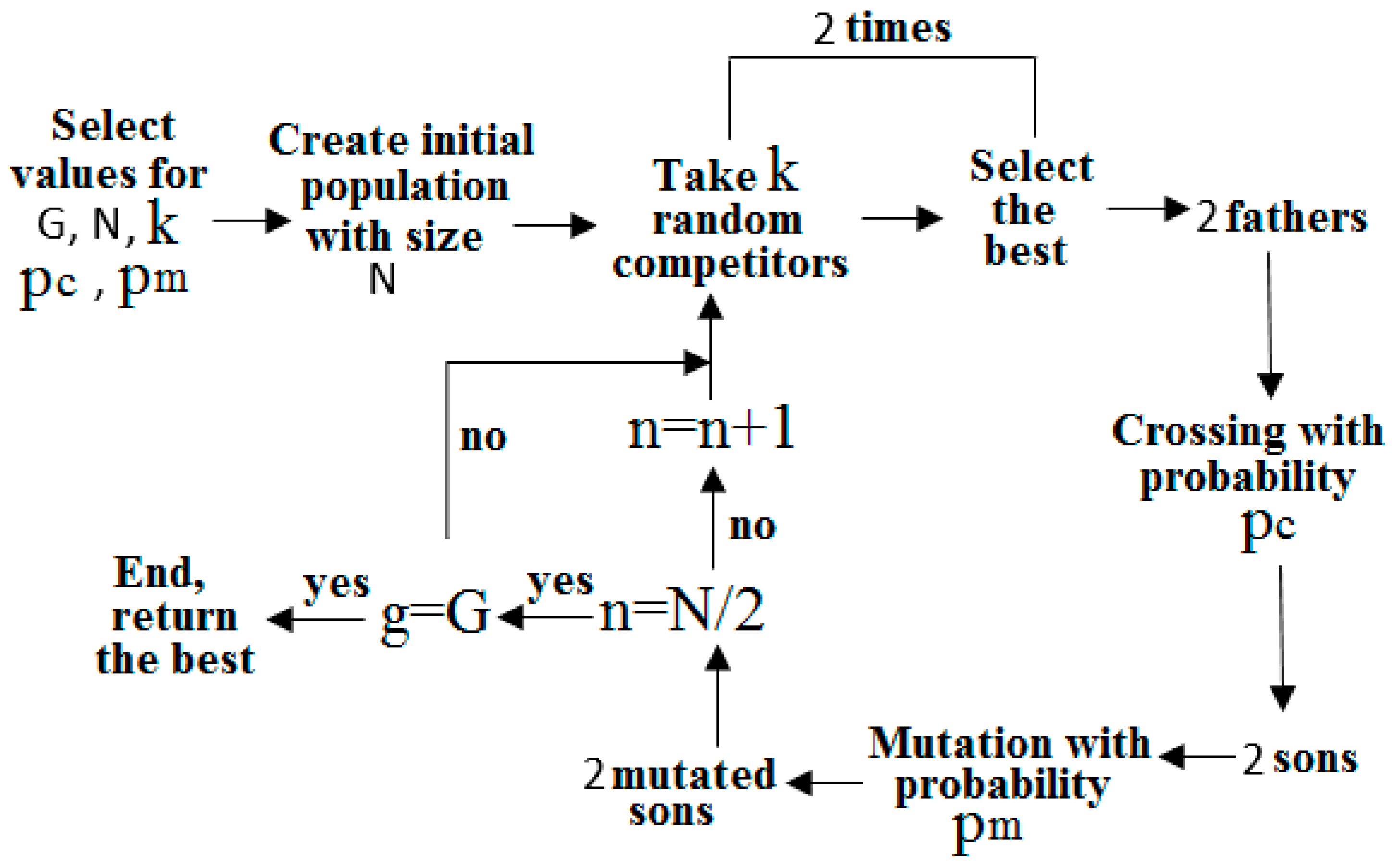
We use the following parameters: $G$ is the generation number, $N$ is the size of the population, $p_c$ is the probability of crossing, $p_m$ is the probability of mutation, $l$ is the size of the chromosome, and $k$ are the competitors in the selection per tournament. The methodology of the algorithm shown in Figure 4 is used to find the best values of the hyper-parameters and it is described as:

(1)

We establish the parameters $G$, $N$, $p_c$, $p_m$, $l$ and $k$.

(2)

We create the random initial population, with size $N$.

(3)

$G=1$, $N=1$.

(4)

We seek the fathers by the selection per tournament.

(5)

We cross the gens (with probability $p_c$) from fathers to sons.

(6)

We mutate the sons with a probability $p_m$.

(7)

We calculate the aptitudes of the mutated sons; we save the aptitude values.

(8)

We repeat the steps from $4$ to $7$, $\frac{N}{2}$ times, ($n=n+1$).

(9)

We find a new generation from the mutated sons.

(10)

$m=m+1$.

(11)

We repeat the steps from $4$ to $10$, $M$ times.

(12)

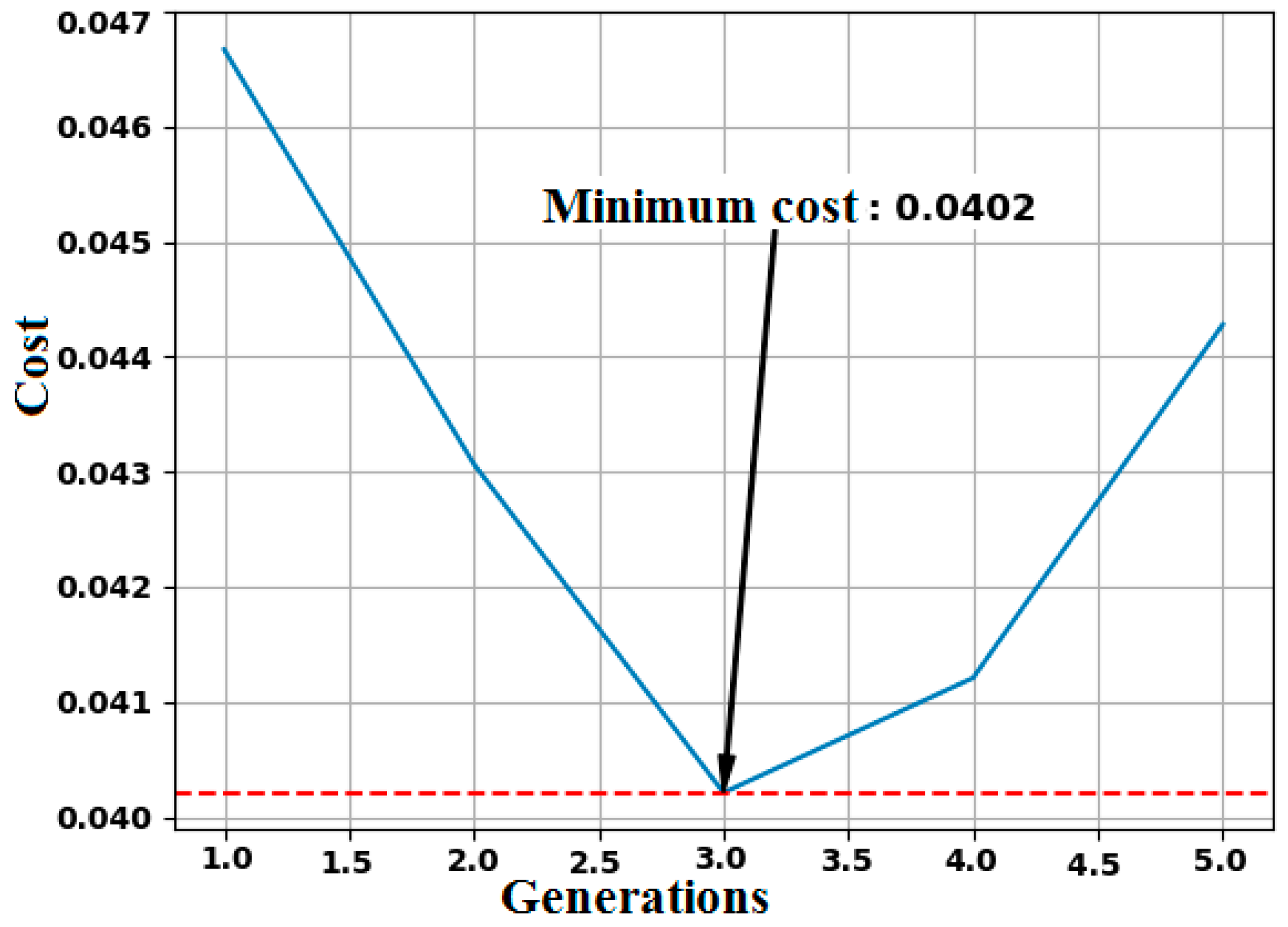
We find the best aptitude from the past generations, or we find the best chromosome in each generation to reach the final response.

3.3. Updating of the Modified Backpropagation

The parameters of the modified backpropagation algorithm are updated with Equations (3) and (4), and with $\beta$ as the momentum constant with a value between $0$ and $1$.

The values considered to find the best values of the hyper-parameters are:

• The width of the Gaussian mapping $\sigma$ is in the interval of $0.1$–$1$.
• The momentum constant $\beta$ is in the interval of $0.9$–$0.99$.
• $p_c=100\%$.
• $p_m=1\%$.
• The population per generation is $60$.
• The number of generations is $5$.
• The value of $k=2$ (k-fold cross-validation).
• The number of competitors is $3$.

We use the methodology described in Figure 4; we create the initial population, for which we propose a solution as a vector with dimension ($1\times 30$); to use the genetic algorithm we need a codified solution:

$$\begin{array}{ccccccccccccccc}1& 1& 1& 1& 0& 0& 0& 0& 1& 1& 1& 1& 0& 0& 0\\ 0& 1& 1& 1& 1& 0& 0& 0& 0& 1& 0& 1& 1& 0& 1\end{array}$$

The first $15$ bits represent the solution of the width in the Gaussian mapping $\sigma$, and the other $15$ bits represent the solution of the momentum constant $\beta$.

From the first solution, to create an initial solution, we randomly mix the elements (bits or gens) $n$ times to find a population of $60$ elements shown in Figure 5 of the width in the Gaussian mapping $\sigma$ and in Figure 6 of the momentum constant $\beta$, it yields a matrix with dimension ($60\times 30$).

Once the initial population is created, we find the fathers and the sons, until we find $5$ generations.

The transcendent part of the algorithm is the evaluation of the chromosomes. Since we find a codified solution, we need to find the decoded solution of the chromosome.

To decode the chromosome, we use the next steps:

(1)

We find the precision of the chromosome. We scale the chromosome in one searching interval $\left[l_{\min },\hspace{0.17em}{l}_{\max }\right]$:

$$P_i=\frac{l_{\max }-l_{\min }}{2^l-1}$$

(5)

with $l$ as the length of the chromosome, $l_{\max }$ is the maximum value of the searching set, and $l_{\min }$ as the minimum value in the searching set.

(2)

The chromosome $D$ is decoded as:

$$D=\left({\displaystyle \sum }_{i=0}^{l-1}{2}^i\right)\times P_i+l_{\min }$$

(6)

Since the first $15$ bits of the chromosome are the width in the Gaussian mapping $\sigma$ and the other $15$ bits are of the momentum constant $\beta$, we find two decimal values in the decoded solution of the chromosome.

As one example, we take into account the next chromosome to find width in the Gaussian mapping $\sigma$ and momentum constant $\beta$.

$$\begin{array}{ccccccccccccccc}1& 1& 1& 1& 0& 0& 0& 0& 1& 1& 1& 1& 0& 0& 0\\ 0& 1& 1& 1& 1& 0& 0& 0& 0& 1& 0& 1& 1& 0& 1\end{array}$$

The first $15$ bits represent the codified solution of the width in the Gaussian mapping $\sigma$. We find the precision in the searching interval with $l_{\min }=0.1$ and $l_{\max }=1$, and the length of the chromosome is $l=15$; then equation (5) is evaluated as:

$$P_i=\frac{l_{\max }-l_{\min }}{2^l-1}=\frac{1-0.1}{2^{15}-1}=2.7467\times {10}^{-5}$$

We find the binary solution $\left({\displaystyle {\displaystyle \sum }_{i=0}^{l-1}}{2}^i\right)$ of (6) as:

$$\begin{array}{c}\left(\begin{array}{ccccccccccccccc}1& 1& 1& 1& 0& 0& 0& 0& 1& 1& 1& 1& 0& 0& 0\end{array}\right)\\ \Rightarrow \left({\displaystyle {\displaystyle \sum }_{i=0}^{l-1}}{2}^i\right)=2^{14}+2^{13}+2^{12}+2^{11}+2^6+2^5+2^4+2^3\\ \Rightarrow \left({\displaystyle {\displaystyle \sum }_{i=0}^{l-1}}{2}^i\right)=30840\end{array}$$

We find the decoded solution of the width in the Gaussian mapping $\sigma$ as:

$$\begin{array}{c}\sigma =\left({\displaystyle {\displaystyle \sum }_{i=0}^{l-1}}{2}^i\right)\times P_i+l_{\min }\\ \Rightarrow \sigma =(30840)(2.7467\times {10}^{-5})+0.1\\ \Rightarrow \sigma =0.94708\end{array}$$

The first $15$ bits represent the codified solution of the momentum constant $\beta$. We find the precision in the searching interval with $l_{\min }=0.9$ and $l_{\max }=0.99$, and the length of the chromosome is $l=15$; then equation (5) is evaluated as:

$$P_i=\frac{l_{\max }-l_{\min }}{2^l-1}=\frac{0.99-0.9}{2^{15}-1}=2.7467\times {10}^{-6}$$

We find the binary solution $\left({\displaystyle {\displaystyle \sum }_{i=0}^{l-1}}{2}^i\right)$ of (6) as:

$$\begin{array}{c}\left(\begin{array}{ccccccccccccccc}0& 1& 1& 1& 1& 0& 0& 0& 0& 1& 0& 1& 1& 0& 1\end{array}\right)\\ \Rightarrow \left({\displaystyle {\displaystyle \sum }_{i=0}^{l-1}}{2}^i\right)=2^{13}+2^{12}+2^{11}+2^{10}+2^5+2^3+2^2+2^0\\ \Rightarrow \left({\displaystyle {\displaystyle \sum }_{i=0}^{l-1}}{2}^i\right)=15405\end{array}$$

We find the decoded solution of the momentum constant $\beta$ as:

$$\begin{array}{c}\beta =\left({\displaystyle {\displaystyle \sum }_{i=0}^{l-1}}{2}^i\right)\times P_i+l_{\min }\\ \Rightarrow \beta =(15405)(2.7467\times {10}^{-6})+0.9\\ \Rightarrow \beta =0.94231\end{array}$$

Thus, for this example, the decoded solution of the width in the Gaussian mapping $\sigma$ is $0.94708$ and the decoded solution of the momentum constant $\beta$ is $0.94231$.

To evaluate the chromosome, we use the next steps:

(1)

With the decoded values of the width in the Gaussian mapping $\sigma$ and of the momentum constant $\beta$, we feed the RBM network. We use the k-fold cross-validation to find a robust model.

(2)

We update the RBM network with the training data $x$ and we find the parameters.

(3)

With the updated values of the RBM network, we evaluate them by using the proof target $y$.

(4)

We generate the modeling with the proof data $x$, which is called $z_3$.

(5)

We compare the data of the target $y$ with the output $z_3$. We use the determination coefficient $R^2$; it is a parameter which determines the quality of the model:

$$R^2=1-\frac{{\displaystyle {\displaystyle \sum }_m}{\left(z_3-\overline{y}\right)}^2}{{\displaystyle {\displaystyle \sum }_m}{\left(y-\overline{y}\right)}^2}$$

(7)

with $z_3$ as the output of the RBM network, $y$ as the target output, $\overline{y}$ as the mean of the target output, and $m$ as the epochs number. $R^2$ generates values from $0$ to $1$. If an algorithm has a precise performance, $R^2$ has values near to $1$, and if an algorithm has an imprecise performance, $R^2$ has values near to $0$.

(6)

We define the cost:

$$FO=1-R^2.$$

(8)

(7)

We define the chromosomes to find the smallest values in the cost (Equation (8)) to reach the most precise performance in the algorithm.

By using the Figure 4, we use the methodology to find the best chromosome. We find the chromosome with the most precise performance in the $G$ proposed generations.

4. Comparisons

In this section we present the comparison between the modified backpropagation of [18,19,20,21], and the genetic algorithm with RBM network of this article for the electricity consumption modeling in a city. The goal is to find a more precise modeling in the electricity consumption. We use the software called Python for all the calculations.

4.1. Description of the Data for the Modeling with the RBM Network

The utilized history data of electricity consumption at each hour and temperature observations of the International Organization for Standardization (ISO) in the Great Britain city [38].

For the electricity consumption modeling, we consider the next eight inputs with data of dimensions $52606\times 8$ for the modeling of the RBM network:

• The temperature of the dry bulb.
• The dew point.
• Hour of the day.
• Day of the week.
• A mark indicating if this is a free or a weekend day.
• Average load of the past day.
• The load of the same hour in the past day.
• The load of the same hour and day in the past week.

Additionally, we utilize one target with data of the load of the same hour and day in the actual week of dimensions 52,606 × 1 for the modeling of the RBM network.

The analysis of this sub-section is used to show that the 52,606 complete data containing eight inputs with data and one target with data are transcendent for the modeling with a RBM network. Since each measure of the 52,606 complete data is updated at each hour (h), the 52,606 complete data of each input and target are physically related to h.

The 52,606 complete data are split in two parts before to the modeling procedure; the first 43,834 dataset is used for the training, being called training data, and the last 8772 dataset is used for the testing, being called testing data. With the training data of (43,834 × 8) for the inputs and (43,834 × 1) for the target, we train the RBM network for the electricity consumption modeling. After of the training stage of the RBM network, with the testing data of (8772 × 8) for inputs and (8772 × 1) for target, we test the RBM network for the electricity consumption modeling.

Table 1. The numerical values for the eight inputs with data and one target with data.

	Count	Mean	Std	Min	25%	50%	75%	Max
BulbT	43,834	50.0716	18.5104	−7	36	51	65	96
dewPoint(°F)	43,834	38.3980	19.6439	−24	24	40	55	75
Hour	43,834	12.4984	6.9224	1	6	12	18	24
Day	43,834	4	2.0003	1	2	4	6	7
Weekend	43,834	0.6890	0.4629	0	0	1	1	1
PaverageLoad	43,834	15,218.2727	2972.5212	9152	12,950	15,411	17,085	28,130
LoadPreviousD	43,834	15,214.8604	2975.7433	9152	12,938.25	15,418	17,087.5	28,130
LoadPreviousW	43,834	15,211.0955	1739.9369	509.5833	14,053.5520	14,953.0416	16,125.9791	23,479.4583
ActualLoad	43,834	15,214.9935	2976.1711	9152	12,936	15,420	17,089	28,130

shows the numerical values for the eight inputs with training data and one target with training data, with count as the number of training data, mean as the mean in the training data, std as the standard deviation of the training data, min as the minimal value of the training data, max as the maximum value of the training data, BulbT(°F) as the temperature of the dry bulb, dewPoint(°F) as the dew point, Weekend as the mark indicating if this is a free or a weekend day, PaverageLoad in MWh as the average load of the past day, LoadPreviousD in MWh as the load of the same hour in the past day, LoadPreviousW in MWh as the load of the same hour and day in the past week, and ActualLoad in MWh as the load of the same hour and day in the actual week.

Figure 7 shows the Pearson relation coefficient called r. The training data are analyzed in groups by two training datasets as follows:

• If r = 1, there is a perfect positive relation between two training datums.
• If 0 < r < 1, there is a positive relation between two training datums.
• If r = 0, there is not relation between two training datums.
• If − 1 < r < 0, there is a negative relation between two training datums.
• If r = −1, there is a perfect negative relation between two training datums.

Since all the values of r are positive, there is a positive relation between all the training data. Additionally, since in the main diagonal r = 1, there is a perfect positive relation between the training data.

Figure 8 shows the relation between all the training data containing the data with numerical values. The training data are grouped by two training datasets; if the slope of the relation is positive, these two training data are related, and if the slope of the relation is negative, these two training data are not related. Since all the slopes are positive, all the training data are related each other. Figure 8 in the main diagonal also shows the distribution of each training input.

The RBM network of Equations (1) and (2) has three parts—one inputs part, one intern part, and one outputs part. The inputs part has eight inputs $a_1$ with the input data, the intern part has six units $a_2=g(z_2)$, and the output part has one output $z_3$ for the modeling of the target output $y$.

4.2. Modified Backpropagation

We use the RBM network of Equations (1) and (2) with the parameters updating of Equations (3) and (4) [18,19,20,21] for the electricity consumption modeling.

We use the momentum to modify the velocity ($V_{d\theta 1}$, $V_{d\theta 2}$) in the modified backpropagation. We train the RBM network with a modeling factor of $\alpha =0.01$; the momentum constant is $\beta =0.9$; the width of the Gaussian mapping is $\sigma =0.3$; the center of the Gaussian mapping is $c=0.0$; we use 100 epochs.

4.3. Genetic Algorithm with RBM Network

First, we define the hyper parameters and find their best values by the genetic algorithm. Second, we use the modified backpropagation with the best hyper-parameters for the modeling.

We use the RBM network of Equations (1) and (2) with the parameter updates of Equations (3) and (4) for the electricity consumption modeling.

To find the best values for the hyper-parameters: we use the width of the Gaussian mapping $\sigma$ in an interval of $0.1$–$1$; the momentum constant $\beta$ in an interval of $0.9$ and $0.99$; the probability of crossing of $100\%$; the probability of mutation of $1\%$; the population per generation of $60$; the number of families of $30$; the number of generations of $5$; the value of $k$ is $2$, (k-fold cross-validation); and the competitors of three. We used the methodology described in Figure 4 and Equations (5)–(8) to find the best values for the RBM network of Equations (1)–(4) for improving the algorithm performance. The genetic algorithm finds the best hyper-parameters for the RBM network of the

Table 2. Hyper-parameters of the genetic algorithm.

Hyper-Parameter	Value
$\sigma$	0.5159
$\beta$	0.9705
	(9)

.

We see in Figure 9 that the best model was found in generation $3$.

We train the RBM network with a modeling factor of $\alpha =0.01$; the momentum constant is $\beta =0.9705$; the width of the Gaussian mapping is $\sigma =0.5159$; the center of the Gaussian mapping is $c=0.0$; we use 100 epochs. We find the next results.

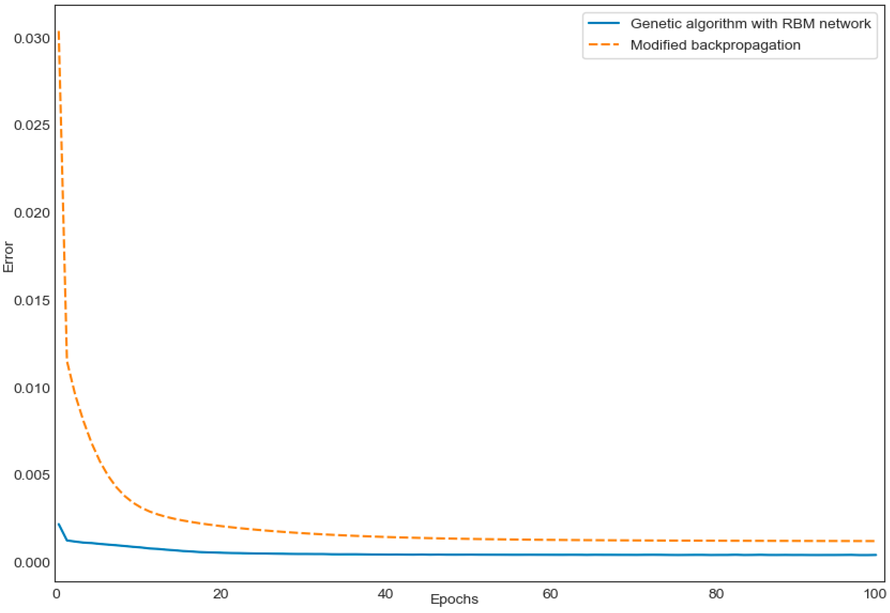
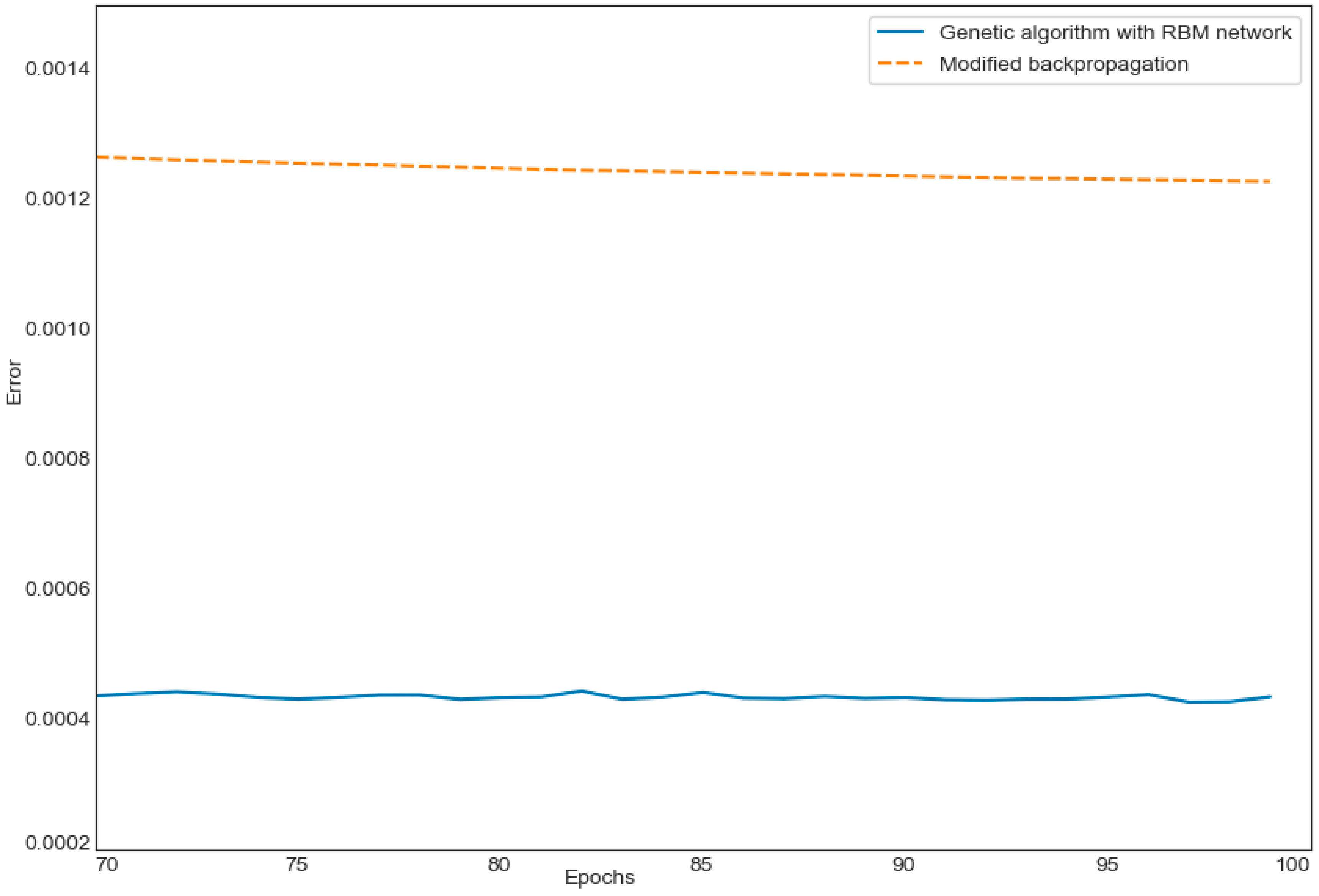
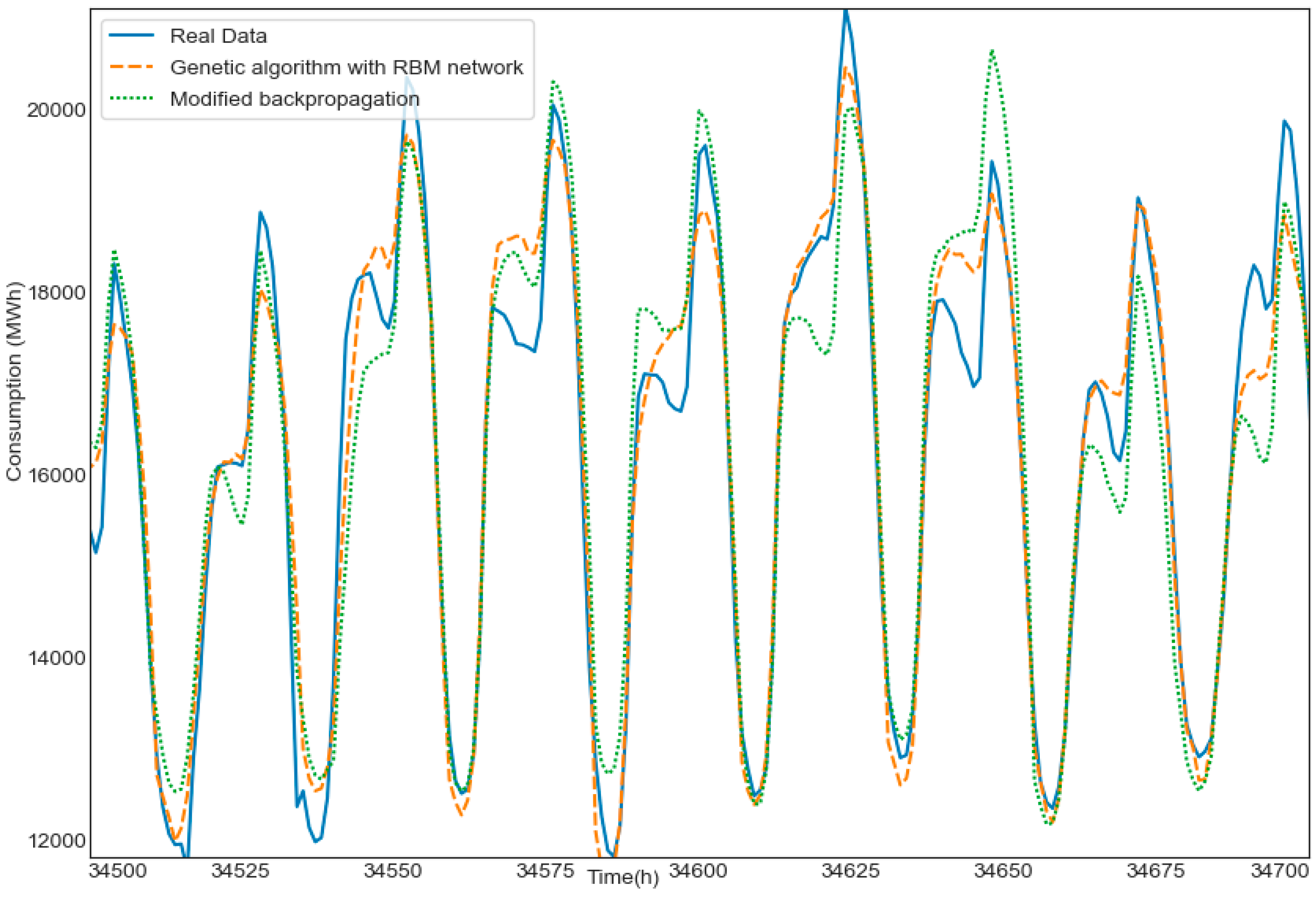
4.4. Comparisons between the Genetic Algorithm with a RBM Network and the Modified Backpropagation

The Figure 10 shows the cost of Equations (7) and (8) for the genetic algorithm with RBM network in comparison with the modified backpropagation during the training. As you can see, the genetic algorithm with RBM network has a more precise modeling than the modified backpropagation during the training, since the RBM network output $z_3$ tends to converge more directly to the target output $y$.

The Figure 11 shows a zoomed-in view of the costs of Equations (7) and (8) for the genetic algorithm with RBM network in comparison with the modified backpropagation during the training after 100 epochs. The genetic algorithm with RBM network has more precise modeling.

The modeling of the genetic algorithm with RBM network of Equations (1)–(8), Figure 4 and Figure 9, and Table 2 in comparison with the modified backpropagation of Equations (1)–(4) during the training is shown in the Figure 12. After 100 epochs, the genetic algorithm with RBM network has a more precise modeling compared to the modified backpropagation.

Figure 13 shows a zoomed-in view of the modeling of the genetic algorithm with RBM network of Equations (1)–(8), Figure 4 and Figure 9, and Table 2 in comparison with the modified backpropagation of Equations (1)–(4) during the training.

After the training, the modeling of the genetic algorithm with RBM network of Equations (1)–(8), Figure 4 and Figure 9, and Table 2 in comparison with the modified backpropagation of Equations (1)–(4) during the testing is shown in the Figure 14.

Figure 15 shows a zoomed-in view of the modeling of the genetic algorithm with RBM network of Equations (1)–(8), Figure 4 and Figure 9, and Table 2 in comparison with the modified backpropagation of Equations (1)–(4) during the testing.

The

Table 3. Comparison results of $R^2$ and cost.

Approaches	${\mathit{R}}^2 \mathbf{Training}$	${\mathit{R}}^2 \mathbf{Testing}$	Cost Training
Hybrid algorithm	0.962	0.941	0.00043
Single algorithm	0.908	0.917	0.00114

compares the results of the genetic algorithm with a RBM network (hybrid algorithm) of Equations (1)–(8), Figure 4 and Figure 9, and Table 2 with the modified backpropagation (single algorithm) of Equations (1)–(4) during the training after 100 epochs. $R^2$ has values between $0$ and $1$; values of $R^2$ close to $1$ correspond to algorithms with more precise modeling results. Since the genetic algorithm with the RBM network has the lowest value in the cost and it has the highest values of $R^2$, it achieves a more precise modeling result.

The

Table 4. Comparison results of mean absolute error (MAE), mean absolute percentage error (MAPE).

Approaches	MAE Testing	MAPE Testing
Hybrid algorithm	543.03 MWh	3.81 %
Single algorithm	604.22 MWh	4.09 %

compares the results between the genetic algorithm with RBM network (hybrid algorithm) of Equations (1)–(8), Figure 4, Figure 9, and Table 2 with the modified backpropagation (Single algorithm) of Equations (1)–(4) for the mean absolute error (MAE) and the mean absolute percentage error (MAPE). Since the genetic algorithm with RBM network has the lowest values in MAE and MAPE, it achieves a more precise modeling result.

5. Conclusions

The goal of this article was modeling the electricity consumption in a city. Then, a hybrid algorithm called genetic algorithm with a RBM network was suggested. The genetic algorithm with a RBM network was compared with the modified backpropagation, since the RBM network output of our algorithm tended to converge more directly to the target output, and with a smaller value in the cost, our algorithm achieved a more precise modeling result. One way in which the modeling by the genetic algorithm with RBM network could serve to improve electricity consumption efficiency is that the same modeling could be used for a better electricity price forecasting [39,40,41,42,43]. The limitation of the suggested approach is that to increase the precision of the modeling, we need to increase the size of the chromosome, or increase the number of generations or evaluated solutions. The next steps are to implement the genetic algorithm in a recurrent neural network or in an autoregressive model.

References

1. Chen, Y.; Luo, F.; Li, T.; Xiang, T.; Liu, Z.; Li, J. A training-integrity privacy-preserving federated learning scheme with trusted execution environment. Inf. Sci. 2020, 522, 69–79. [Google Scholar] [CrossRef]
2. Egrioglu, E.; Bas, E.; Yolcu, U.; Chen, M.-Y. Picture fuzzy time series: Defining, modeling and creating a new forecasting method. Eng. Appl. Artif. Intell. 2020, 88, 103367. [Google Scholar] [CrossRef]
3. Jia, B.; Xu, H.; Liu, S.; Li, W. A High Quality Task Assignment Mechanism in Vehicle-Based Crowdsourcing Using Predictable Mobility Based on Markov. IEEE Access 2018, 6, 64920–64926. [Google Scholar] [CrossRef]
4. Zhang, X.; Yang, S.; Srivastava, G.; Chen, M.-Y.; Cheng, X. Hybridization of cognitive computing for food services. Appl. Soft Comput. 2020, 89, 106051. [Google Scholar] [CrossRef]
5. Chang, J.-R.; Chen, M.-Y.; Chen, L.-S.; Tseng, S.-C. Why Customers Don’t Revisit in Tourism and Hospitality Industry? IEEE Access 2019, 7, 146588–146606. [Google Scholar] [CrossRef]
6. Dinculeană, D.; Cheng, X. Vulnerabilities and Limitations of MQTT Protocol Used between IoT Devices. Appl. Sci. 2019, 9, 848. [Google Scholar] [CrossRef] [Green Version]
7. Sangaiah, A.K.; Pham, H.; Chen, M.-Y.; Lu, H. Mercaldo, F. Cognitive data science methods and models for engineering applications. Soft Comput. 2019, 23, 9045–9048. [Google Scholar] [CrossRef] [Green Version]
8. Shi, F.; Chen, Z.; Cheng, X. Behavior Modeling and Individual Recognition of Sonar Transmitter for Secure Communication in UASNs. IEEE Access 2020, 8, 2447–2454. [Google Scholar] [CrossRef]
9. Chiang, H.-S.; Chen, M.-Y.; Huang, Y.-J. Wavelet-Based EEG Processing for Epilepsy Detection Using Fuzzy Entropy and Associative Petri Net. IEEE Access 2019, 7, 103255–103262. [Google Scholar] [CrossRef]
10. Sadiq, M.; Shi, D.; Guo, M.; Cheng, X. Facial Landmark Detection via Attention-Adaptive Deep Network. IEEE Access 2019, 7, 181041–181050. [Google Scholar] [CrossRef]
11. Wang, C.; Yao, H.; Liu, Z. An efficient DDoS detection based on SU-Genetic feature selection. Clust. Comput. 2018, 22, 2505–2515. [Google Scholar] [CrossRef]
12. Chen, M.-Y.; Chiang, H.-S.; Sangaiah, A.K.; Hsieh, T.-C. Recurrent neural network with attention mechanism for language model. Neural Comput. Appl. 2019, 32, 7915–7923. [Google Scholar] [CrossRef]
13. Jia, B.; Hao, L.; Zhang, C.; Chen, D. A Dynamic Estimation of Service Level Based on Fuzzy Logic for Robustness in the Internet of Things. Sensors 2018, 18, 2190. [Google Scholar] [CrossRef] [PubMed] [Green Version]
14. Wang, C.; Yang, L.; Wu, Y.; Wu, Y.; Cheng, X.; Li, Z.; Liu, Z. Behavior Data Provenance with Retention of Reference Relations. IEEE Access 2018, 6, 77033–77042. [Google Scholar] [CrossRef]
15. Xie, T.; Yu, H.; Wilamowski, B. Comparison between traditional neural networks and radial basis function networks. In Proceedings of the 2011 IEEE International Symposium on Industrial Electronics, Gdansk, Poland, 27–30 June 2011; pp. 1194–2013. [Google Scholar] [CrossRef]
16. Xie, T.; Yu, H.; Hewlett, J.; Rózycki, P.; Wilamowski, B. Fast and efficient second-order method for training radial basis function networks. IEEE Trans. Neural Netw. Learn. Syst. 2012, 23, 609–619. [Google Scholar] [CrossRef]
17. Yu, H.; Reiner, P.D.; Xie, T.; Bartczak, T.; Wilamowski, B.M. An Incremental Design of Radial Basis Function Networks. IEEE Trans. Neural Netw. Learn. Syst. 2014, 25, 1793–1803. [Google Scholar] [CrossRef]
18. Manukian, H.; Traversa, F.L.; Di Ventra, M. Accelerating deep learning with memcomputing. Neural Netw. 2019, 110, 1–7. [Google Scholar] [CrossRef] [Green Version]
19. Rubio, J.D.J.; Cruz, D.R.; Elias, I.; Ochoa, G.; Balcazar, R.; Aguilar, A.; Balcazarand, R. ANFIS system for classification of brain signals. J. Intell. Fuzzy Syst. 2019, 37, 4033–4041. [Google Scholar] [CrossRef]
20. Wang, X.; Qin, Y.; Zhang, A. An intelligent fault diagnosis approach for planetary gearboxes based on deep belief networks and uniformed features. J. Intell. Fuzzy Syst. 2018, 34, 3619–3634. [Google Scholar] [CrossRef]
21. Wen, Z.; Xie, L.; Feng, H.; Tan, Y. Robust fusion algorithm based on RBF neural network with TS fuzzy model and its application to infrared flame detection problem. Appl. Soft Comput. 2019, 76, 251–264. [Google Scholar] [CrossRef]
22. Kapanova, K.; Dimov, I.; Sellier, J.M. A genetic approach to automatic neural network architecture optimization. Neural Comput. Appl. 2016, 29, 1481–1492. [Google Scholar] [CrossRef]
23. Metawa, N.; Hassan, M.K.; Elhoseny, M. Genetic algorithm based model for optimizing bank lending decisions. Expert Syst. Appl. 2017, 80, 75–82. [Google Scholar] [CrossRef]
24. Shojaedini, E.; Majd, M.; Safabakhsh, R. Novel adaptive genetic algorithm sample consensus. Appl. Soft Comput. 2019, 77, 635–642. [Google Scholar] [CrossRef] [Green Version]
25. Yegireddy, N.K.; Panda, S.; Papinaidu, T.; Yadav, K.P.K. Multi-objective non dominated sorting genetic algorithm-II optimized PID controller for automatic voltage regulator systems. J. Intell. Fuzzy Syst. 2018, 35, 4971–4975. [Google Scholar] [CrossRef]
26. Nazarahari, M.; Khanmirza, E.; Doostie, S. Multi-objective multi-robot path planning in continuous environment using an enhanced genetic algorithm. Expert Syst. Appl. 2019, 115, 106–120. [Google Scholar] [CrossRef]
27. Orozco-Rosas, U.; Montiel, O.; Sepúlveda, R. Mobile robot path planning using membrane evolutionary artificial potential field. Appl. Soft Comput. 2019, 77, 236–251. [Google Scholar] [CrossRef]
28. Saini, R.; Roy, P.P.; Dogra, D.P. A segmental HMM based trajectory classification using genetic algorithm. Expert Syst. Appl. 2018, 93, 169–181. [Google Scholar] [CrossRef]
29. Tseng, H.-E.; Chang, C.-C.; Lee, S.-C.; Huang, Y.-M. A Block-based genetic algorithm for disassembly sequence planning. Expert Syst. Appl. 2018, 96, 492–505. [Google Scholar] [CrossRef]
30. Arghish, O.; Tavakkoli-Moghaddam, R.; Shahandeh-Nookabadi, A.; Rezaeian, J. An integrated cellular manufacturing system with type-2 fuzzy variables: Three tuned meta-heuristic algorithms. J. Intell. Fuzzy Syst. 2018, 35, 2293–2308. [Google Scholar] [CrossRef]
31. Gola, A.; Kłosowski, G. Development of computer-controlled material handling model by means of fuzzy logic and genetic algorithms. Neurocomputing 2019, 338, 381–392. [Google Scholar] [CrossRef]
32. Kuo, R.J.; Quyen, N.T.P. Genetic intuitionistic weighted fuzzy k-modes algorithm for categorical data. Neurocomputing 2019, 330, 116–126. [Google Scholar] [CrossRef]
33. Pei, X.; Zhou, Y.; Wang, N. A Gaussian process regression based on variable parameters fuzzy dominance genetic algorithm for B-TFPMM torque estimation. Neurocomputing 2019, 335, 153–169. [Google Scholar] [CrossRef]
34. Armaghani, D.J.; Hasanipanah, M.; Mahdiyar, A.; Majid, M.Z.A.; Amnieh, H.B.; Tahir, M.M.D. Airblast prediction through a hybrid genetic algorithm-ANN model. Neural Comput. Appl. 2016, 29, 619–629. [Google Scholar] [CrossRef]
35. Harkat, H.; Ruano, A.; Ruano, M.; Dosse, S.B. GPR target detection using a neural network classifier designed by a multi-objective genetic algorithm. Appl. Soft Comput. 2019, 79, 310–325. [Google Scholar] [CrossRef]
36. Karami, H.; Karimi, S.; Bonakdari, H.; Shamshirband, S. Predicting discharge coefficient of triangular labyrinth weir using extreme learning machine, artificial neural network and genetic programming. Neural Comput. Appl. 2016, 29, 983–989. [Google Scholar] [CrossRef]
37. Sayed, S.; Nassef, M.; Badr, A.; Farag, I. A Nested Genetic Algorithm for feature selection in high-dimensional cancer Microarray datasets. Expert Syst. Appl. 2019, 121, 233–243. [Google Scholar] [CrossRef]
38. Electricity Load and Price Forecasting with MATLAB. Available online: https://www.mathworks.com/videos/electricity-load-and-price-forecasting-with-matlab-81765.html (accessed on 8 September 2010).
39. Cincotti, S.; Gallo, G.; Ponta, L.; Raberto, M. Modeling and forecasting of electricity spot-prices: Computational intelligence vs. classical econometrics. AI Commun. 2014, 27, 301–314. [Google Scholar] [CrossRef]
40. Gallo, G. Electricity market games: How agent-based modeling can help under high penetrations of variable generation. Electr. J. 2016, 29, 39–46. [Google Scholar] [CrossRef] [Green Version]
41. Janczura, J.; Weron, R. An empirical comparison of alternate regime-switching models for electricity spot prices. Energy Econ. 2010, 32, 1059–1073. [Google Scholar] [CrossRef] [Green Version]
42. Weron, R. Electricity price forecasting: A review of the state-of-the-art with a look into the future. Int. J. Forecast. 2014, 30, 1030–1081. [Google Scholar] [CrossRef] [Green Version]
43. Weron, R.; Misiorek, A. Forecasting spot electricity prices: A comparison of parametric and semiparametric time series models. Int. J. Forecast. 2008, 24, 744–763. [Google Scholar] [CrossRef] [Green Version]
Figure 1. The radial basis mapping (RBM) network.
Applsci 10 04239 g001
Figure 2. The modified backpropagation.
Applsci 10 04239 g002
Figure 3. The k-fold cross-validation.
Applsci 10 04239 g003
Figure 4. Flow diagram of the genetic algorithm.
Applsci 10 04239 g004
Figure 5. The first 30 codified solutions of the width in the Gaussian mapping.
Applsci 10 04239 g005
Figure 6. The first 30 codified solutions of the momentum constant.
Applsci 10 04239 g006
Figure 7. The Pearson relation between the training data.
Applsci 10 04239 g007
Figure 8. The relation between the training data.
Applsci 10 04239 g008
Figure 9. Cost mapping of the genetic algorithm.
Applsci 10 04239 g009
Figure 10. Cost of algorithms during training.
Applsci 10 04239 g010
Figure 11. A zoomed-in view of the costs of algorithms during the training.
Applsci 10 04239 g011
Figure 12. Modeling of algorithms during the training.
Applsci 10 04239 g012
Figure 13. A zoomed-in view of the modeling of algorithms during the training.
Applsci 10 04239 g013
Figure 14. Modeling of algorithms during the testing.
Applsci 10 04239 g014
Figure 15. A zoomed-in view of the modeling of algorithms during the testing.
Applsci 10 04239 g015