6.1. Optimization and Computational Results
Due to the stochastic and irreproducible nature of optimization algorithms, validating their performance is supposed to be via statistical analysis on the goodness of the found solutions of several trials. Thus, the suggested particle swarm optimization algorithm has been simulated 20 times with a maximum Number of Improvisations (iterations) = 100 and a Harmony Memory Size = 20 while running on an Intel Core i5, 3.30 GHz CPU. Feasible solutions have been obtained in 80% of trials and in acceptable CPU calculation time.
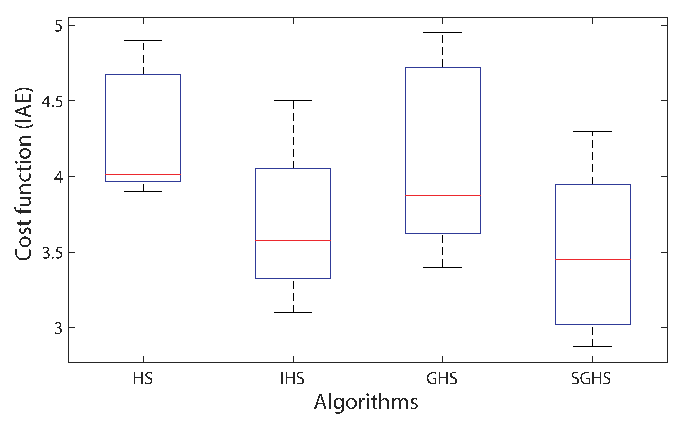
Figure 11 illustrates the box-and-whisker plot of the results of the optimization of all four variants of the Harmony Search algorithm (i.e., HS, IHS, GHS, SGHS) for Problem (
18).
The figure shows that the obtained solutions from all four algorithms are in the same region of the search space. From a statistical point of view, we focus on the average values which are 4.015, 3.575, 3.875, and 3.450 for HS, HIS, GHS and SGHS, respectively. However, in general, it is obvious that, in terms of average value (red line) and of minimum value (bottom whisker), among 20 trials of every algorithm the SGHS algorithm presents superiority over the previous variants. However, it is to be noted that the box of the IHS algorithm is the narrowest which is thanks to its pitch adjustment rules that favor exploitation and precision. On the other hand, the GHS show less favorable results with wider box, meaning dispersed solutions, this may be due to the lack of solution refinement via the parameter.
The significant outcomes of the 20 trials using all four algorithms are detailed in
Table 2. The SGHS algorithm is the best in terms of average value but not significantly better. SGHS has the lowest minimum, maximum, median and mean values and the HS algorithm has the lowest standard deviation.
To further understand the behavior of the algorithms
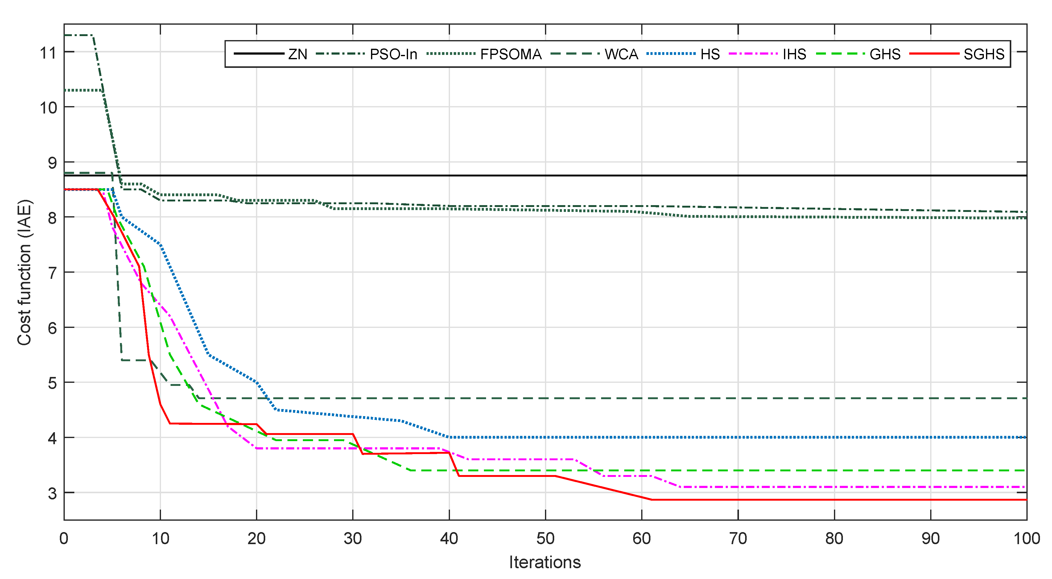
Figure 12 illustrates the most typical convergence curves of HS, IHS, GHS and SGHS along with the curves of previously tested algorithms—the Particle Swarm Optimization with decreasing inertia (PSO-In), the Fractional-Order Particle Swarm Optimization Memetic Algorithm (FPSOMA) and the Water Cycle Algorithm (WCA).
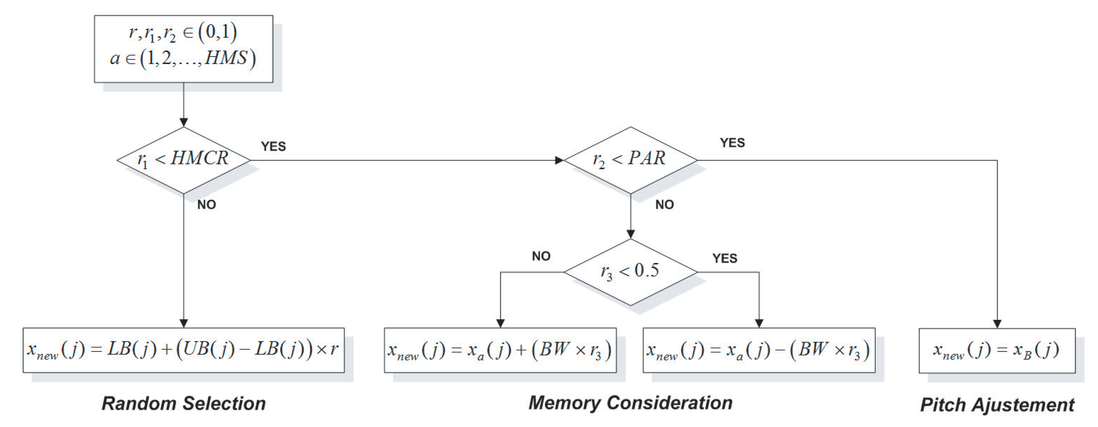
From the convergence histories, it can be noticed that all algorithms successfully converge to the same region of the search space (between 3 and 4) but the optimal is from the SGHS algorithm. The other variants of the HS algorithm managed to enhance the exploration and exploitation capabilities but with different outcomes. In the case of the IHS algorithm, the precision has been improved thanks to the increase of the exploitation with the new pitch adjustment rules (
21) and (
22) but because
continues to increase until the end, somehow IHS diverged from the optimal region. In the case of the GHS algorithm, it converged quicker to the best solution thanks to the use of the best vector in the improvisation process, however, the GHS failed to further converge because of the lack of refinement rules using
this behavior is known as the premature convergence. Finally, in the case of the SGHS algorithm, it can be noticed that a gradual convergence took place thanks to the self-adaptation of
and
every
improvisations. Moreover, the reinstatement of the refinement rules using the bandwidth parameter
allowed SGHS to obtain more precise solutions than those of the IHS algorithm. The Water Cycle Algorithm presents close results to the HS algorithm, but the new variants of the HS algorithm are better in comparison to other previous algorithms tested on the OWC system.
The parameters obtained from the mean case of feasible results from 20 trials of optimization using the HS, IHS, GHS and SGHS algorithms are given in
Table 3. The
,
and
values are within a close range, proving that the algorithms converge to the same interesting search region.
6.2. OWC Performance Evaluation
For the assessment of the performance of the suggested airflow-control on the OWC system, the optimized PID controller using the parameters found of the mean case of the SGHS optimization results. The evaluation compares the performance of the uncontrolled OWC, the OWC using a traditionally tuned PID using the well known Ziegler–Nichols method (ZN-PID) and the OWC using the optimized PID with SGHS algorithm (SGHS-PID) with the parameters given in
Table 3.
6.2.1. Performance With Regular Waves
During the simulations, two regular wave conditions were considered the first wave is weak with a wave period
T =
and a wave amplitude
A =
from
to
. From
to
, we considered a stronger wave with a wave period
T =
and a wave amplitude
A =
as shown in
Figure 13.
The flow coefficients of the OWC in the uncontrolled case and with the airflow control using the traditionally tuned PID (ZN-PID) and the optimized PID (SGHS-PID) are illustrated in
Figure 14.
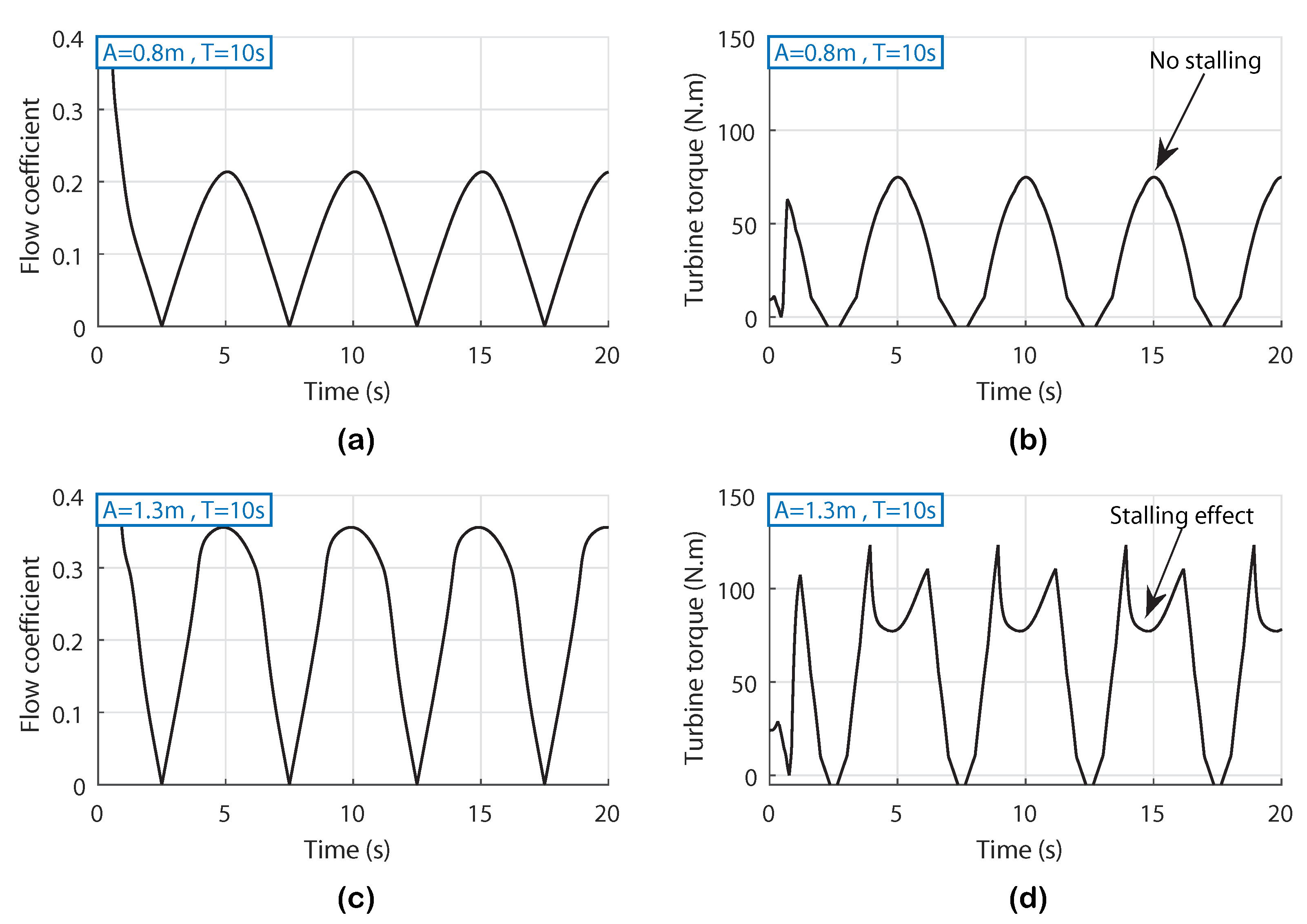
The figure shows that in the uncontrolled case the flow coefficient surpasses the threshold value 0.3 which will provoke the stall effect, whereas in both controlled cases the flow coefficients were regulated below 0.3 thanks to both ZN-PID and SGHS-PID controllers. However, when zooming to the curves it is observed that the SGHS-PID manages to provide a closer flow coefficient to the threshold value than that of the ZN-PID.
Figure 15 shows that in the uncontrolled case, the airflow speed continues to increase; however, in both controlled cases, the airflow speed decreased thanks to both ZN-PID and SGHS-PID controllers, but with a slight superiority for the SGHS-PID.
The obtained turbine torques of the PTO in the uncontrolled case, ZN-PID controller and SGHS-PID controller are shown in
Figure 16a,
Figure 16c,e, respectively. Furthermore, the generated powers for the uncontrolled case, ZN-PID controller and SGHS-PID controller are shown in
Figure 16b,
Figure 16d,f, respectively.
It may be observed that during the uncontrolled case the torque has been affected by the stall effect which reduced it in terms of average value to . On the other hand, the airflow control manages to avoid the stall effect and increase the torques in terms of average values to and for ZN-PID and SGHS-PID, respectively. As a result from the obtained torques, the generated powers in the uncontrolled case is the lowest with and the highest power is generated when using the SGHS-PID with followed by when using a ZN-PID in the proposed airflow control scheme.
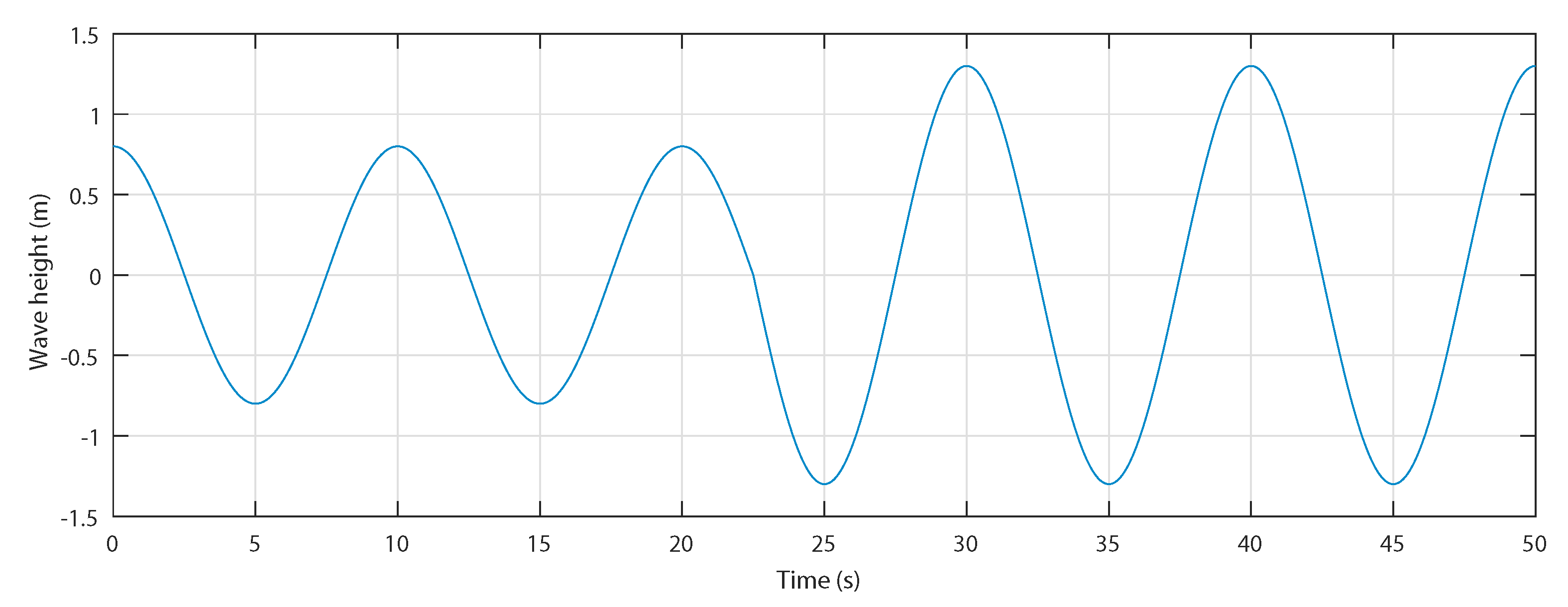
6.2.2. Performance with Real Wave Data
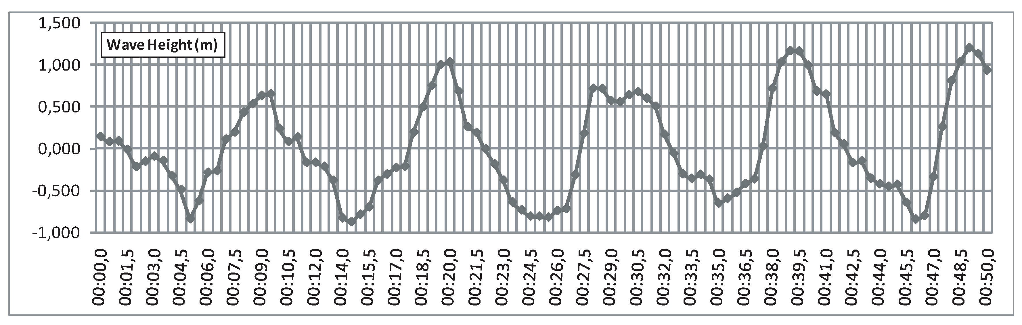
For this study case, real surface elevation measurements of waves in Mutriku obtained by the Acoustic Doppler Current Profiler on 12 May 2014, from 00:00:00 a.m. to 00:00:50 a.m., shown in
Figure 17, were considered.
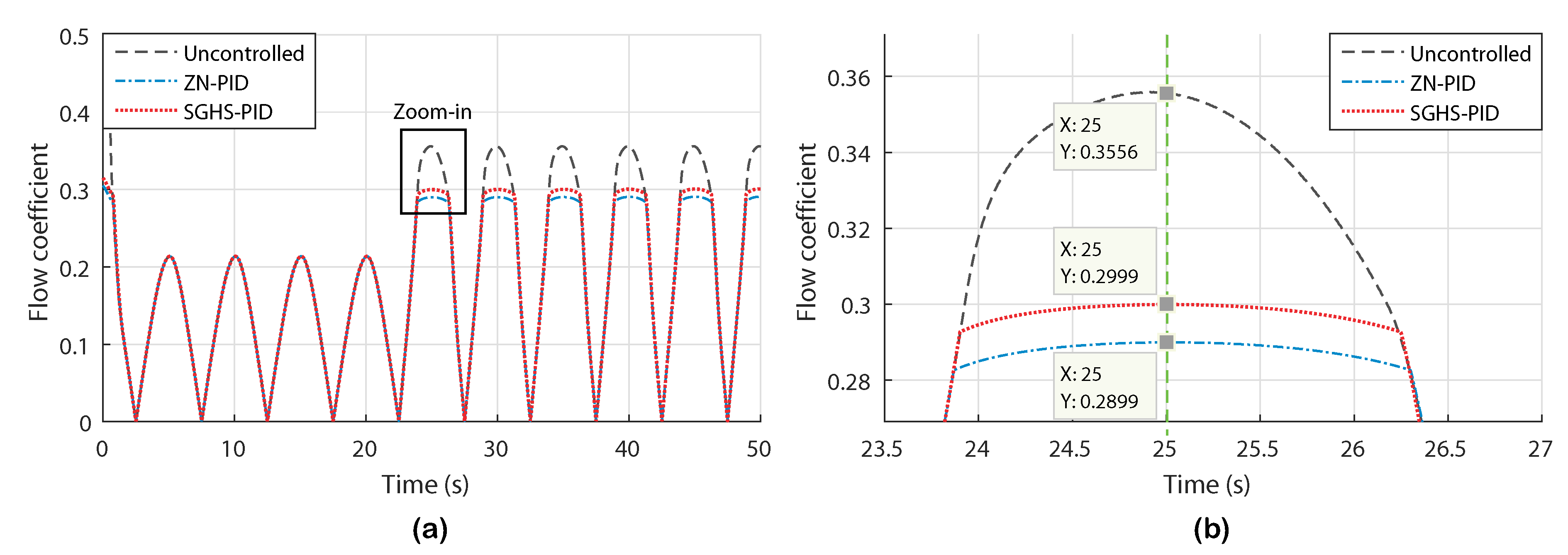
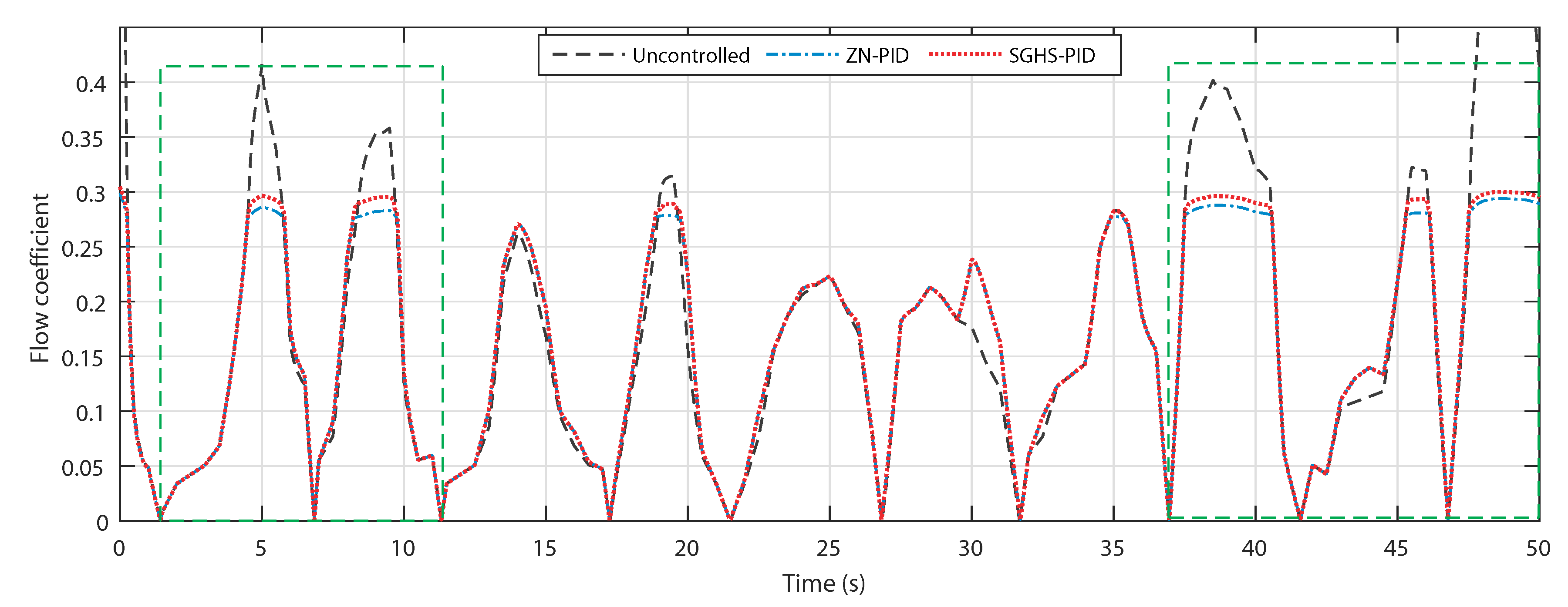
The flow coefficients of the OWC with real measured wave data input in the uncontrolled case, and with airflow control using the traditionally tuned PID (ZN-PID) and the optimized PID (SGHS-PID), are illustrated in
Figure 18.
Figure 18 shows that in the uncontrolled case, the flow coefficient exceeds the threshold value 0.3, which will provoke the stall effect in two time periods with strong waves. The first wave train is from 2 s to 11 s and the second strong wave train is from 37 s to 50 s. In both controlled cases, the flow coefficients were regulated below 0.3 thanks to both ZN-PID and SGHS-PID controllers, with a slight superiority for SGHS-PID.
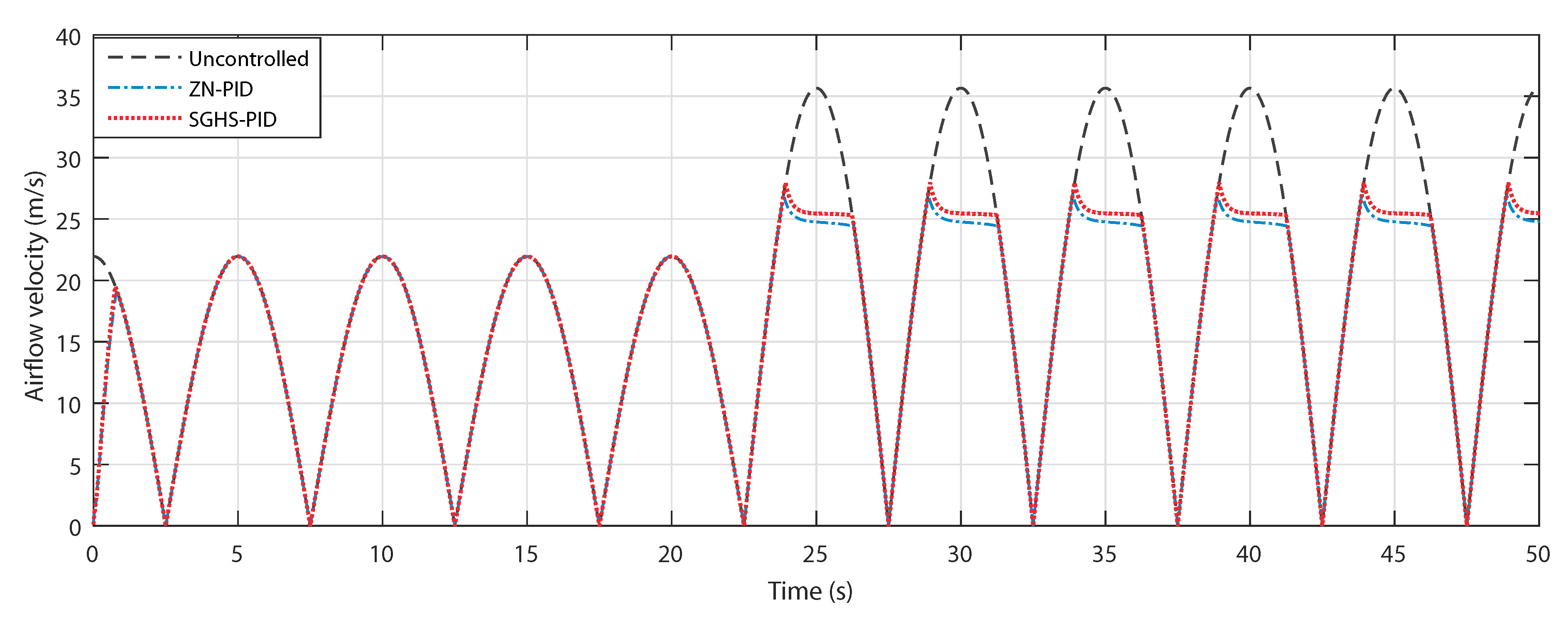
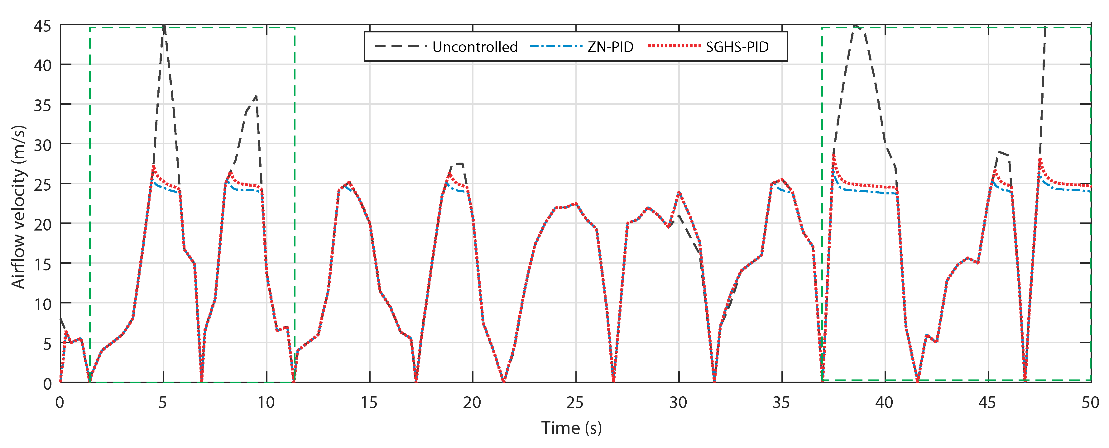
Figure 19 shows that in the uncontrolled case, the airflow speed continues to increase uncontrollably in both periods of the strong waves; however, in both controlled cases, the airflow speed was decreased thanks to both ZN-PID and SGHS-PID controllers, but with a slight superiority for SGHS-PID.
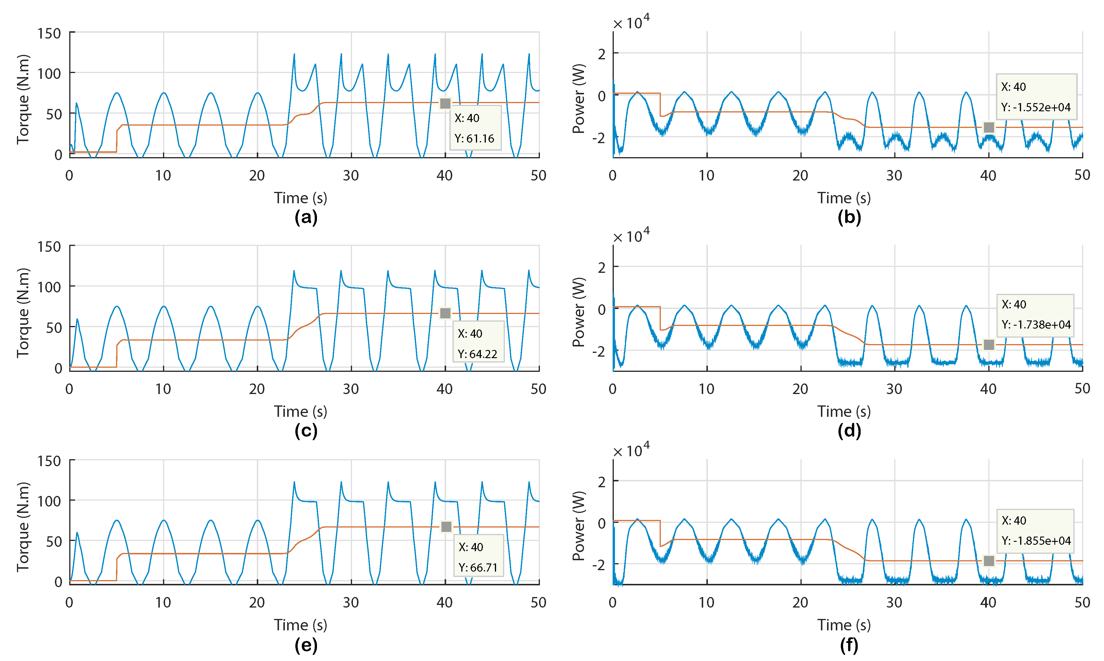
The obtained turbine torques of the PTO in the uncontrolled case, ZN-PID controller and SGHS-PID controller are shown in
Figure 20a,c,e, respectively. And the generated powers for the uncontrolled case, ZN-PID controller and SGHS-PID controller are shown in
Figure 20b,
Figure 20d,f, respectively.
As with regular waves, it may be observed that during the uncontrolled case, the torque has been affected by the stall effect, which reduces it in terms of average value. On the other hand, the airflow control manages to avoid the stall effect and increase the torques in terms of average values in both high wave regions. The resulting generated powers in the uncontrolled case is the lower than the powers generated when using the SGHS-PID and the ZN-PID in the proposed airflow control scheme.


