An Efficient Lossless Compression Method for Periodic Signals Based on Adaptive Dictionary Predictive Coding

Abstract

This paper reports on an efficient lossless compression method for periodic signals based on adaptive dictionary predictive coding. Some previous methods for data compression, such as difference pulse coding (DPCM), discrete cosine transform (DCT), lifting wavelet transform (LWT) and KL transform (KLT), lack a suitable transformation method to make these data less redundant and better compressed. A new predictive coding approach, basing on the adaptive dictionary, is proposed to improve the compression ratio of the periodic signal. The main criterion of lossless compression is the compression ratio (CR). In order to verify the effectiveness of the adaptive dictionary predictive coding for periodic signal compression, different transform coding technologies, including DPCM, 2-D DCT, and 2-D LWT, are compared. The results obtained prove that the adaptive dictionary predictive coding can effectively improve data compression efficiency compared with traditional transform coding technology.

1. Introduction

With the popularization of digitalization, computers and data processing equipment have penetrated into all walks of life, and analog communication has almost been replaced by digital communication. People are faced with the rapid growth of mass information, and the increasing amount of data transmitted, processed and stored has caused great pressure on the transmission bandwidth, storage capacity and processing speed. For example, the Fuji Electric’s PowerSataliteII measurement terminal recorded a power quality fault of 2 s in length, and the generated recording file was 948 kB. It can be seen from this that the huge amount of data takes up a lot of limited storage space and network resources. Therefore, researching efficient data compression methods that reduce the redundancy existing in massive data has become an urgent need in many modern industries. This includes power quality signal compression in the power industry and ECG signal compression in the medical industry, which are periodic signals or quasi-periodic signals.

Data compression is the smallest digital representation of the signal sent by the source, reducing the signal space that contains a given message set or data sampling set. The general steps of data compression and decompression are shown in Figure 1. The compression process mainly includes three steps: transform coding [1,2,3], quantization, and entropy coding [4,5,6,7] or dictionary compression [8,9]. The decompression process mainly includes three steps: entropy decoding or dictionary decompression, inverse quantization, and inverse transform.

An, Q proposed a data compression method for power quality monitoring based on two-dimensional discrete cosine transform (DCT), which converts one-dimensional data into two-dimensional data for data compression [10]. Zhang, R proposed a new three-phase power quality data compression method based on wavelet transform, which, combined with Lempel-Ziv-Welch (LZW) coding, achieves a good compression effect on power quality signal compression [11]. Tsai, T proposed a multi-channel lossless ECG compression algorithm that uses exponentially weighted multi-channel linear prediction and adaptive Golomb-Rice coding [12]. Alam, S proposed a DPCM-based threshold data compression technology for real-time remote monitoring applications, which uses simple calculation and a high compression ratio [13]. Liu, B demonstrated a unified GAN based signal compression framework for image and speech signals [14]. Wang, I proposed a framework of combining machine learning based classification and pre-existing coding algorithms, along with a novel revamp of using DPCM for DWT coefficients [15]. In order to improve the accuracy of prediction, Huang, F proposed a novel ECG signal prediction method based on the autoregressive integrated moving average (ARIMA) model and discrete wavelet transform (DWT) [16]. Suhartono proposed a hybrid spatio-temporal model by combining the generalized space–time autoregressive with exogenous variable and recurrent neural network (GSTARX-RNN) for space–time data forecasting with calendar variation effect [17].

The pattern matching predictor has been studied for a long time with many results. Jacquet, P proposed a universal predictor based on pattern matching, called the sampled pattern matching (SPM), which is a modification of the Ehrenfeucht–Mycielski pseudorandom generator algorithm [18]. Although SPM has a good prediction ability for periodic signals, it involves pattern matching. The complexity of the algorithm is increased by the matching of the maximal suffix, which makes the real-time performance of the algorithm worse. Feder, M proposed the FS predictor, which can calculate the minimum fraction of prediction errors [19]. The FS predictor mainly predicts binary sequences. For multi-bit wide digital sequences, its complexity is high.

Data signals generally have strong time redundancy, but there are more characters in the signal and the distribution probability of characters is relatively uniform. If entropy coding or dictionary compression is directly used to compress data signals, not only is the compression ratio low, but the compression time is also long, which cannot meet the compression requirements. If we can group similar contexts together, the symbols that follow them are likely to be the same, and a very simple and efficient compression strategy can be exploited. Among context-based algorithms, the most famous is the partial matching prediction (PPM) algorithm, which was first proposed by Cleary and Witten [20] in 1984. For time-series signals, the ARIMA model and RNN model can accurately predict, but their algorithm complexity is high, so they are mostly used for time series with low real-time requirements such as air temperature and wind speed. Unfortunately, in the process of data compression, massive data prediction is required, and the ARIMA model and the RNN model take a lot of time. Therefore, they do not meet the real-time requirements of data compression [18,19].

To solve the problem of periodic signal compression, we propose an efficient lossless compression method for periodic signals based on the adaptive dictionary. According to the data value of the past, the dictionary model is used to predict the current data value. The prediction coding usually does not directly code the signal, but codes the prediction error. Because the adaptive dictionary predictive coding concentrates most of the data in a small amount of data, it effectively reduces the amount of data to obtain a high compression ratio.

2. Algorithm Introduction

2.1. Coding Algorithm Introduction

As shown in Figure 2, it is assumed that a sequence $\left\{s(k)\right\}$ ($k$ = 1, 2, …, n) is given. Each symbol $s(k)$ belong to a finite digital sequence $e(k)$ is the output of the coding process. In the periodic signal, there is a great correlation between the different periods of the signal; therefore, the multivariate digital group of the periodic signal, such as the ternary group (s(k − 2),s(k − 1),s(k)), will have great repeatability. When a periodic signal is predicted, the history information of the signal is important. We built a dictionary to store the history information of the signal. Because the history information of the signal is rich. According to the characteristics of the periodic signal, the adaptive dictionary is only used to store the information of the above ternary groups. In this way, not only can the periodic signal can be accurately predicted, but the size of the dictionary is not very large and it is easy to implement it in the project. In order to reduce the complexity of querying the dictionary, for a ternary digit group (s(k − 2),s(k − 1),s(k)), the first two digits s(k − 2) and s(k − 1) are used to store the two-dimensional address of s(k). Although this is not unique mapping and will cause memory conflicts, the complexity of the dictionary lookup algorithm is low, just $O(1)$. When a memory conflict is encountered, the current ternary group directly overwrites the previous ternary group. In this way, the dictionary created by us will be dynamic, which is adaptive. Furthermore, the larger the dimension of the adaptive dictionary, the lower the probability of the memory conflicts. However, as the dictionary dimension increases, the storage size of the dictionary will increase dramatically. The storage size of the high-dimensional dictionary will be unacceptable to us. Therefore, the two-dimensional dictionary will be our best choice. Before introducing the algorithm, we introduce a definition:

(1) We define $s(k-2)$, $s(k-1)$ as the first two adjacent digitals of $s(k)$.

First, the two-dimensional dictionary $D$ is created, whose size is $n\times n$. The coded digitals are then stored in the adaptive dictionary. The position of the digital in the dictionary is the two-dimensional coordinate formed by the first two adjacent digitals $s(k-2)$ and $s(k-1)$. Then the current digital $s(k)$, whose first two adjacent digitals make up the address ($s(k-2)$, $s(k-1)$), is coded, and the predicted value $s^{\prime }(k)$ of the current digital to be coded is read in the dictionary $D$ ($s(k-2)$, $s(k-1)$). Then the current coded digital $s(k)$ is subtracted from the predicted value $s^{\prime }(k)$ to obtain an error signal $e(k)=s(k)-s^{\prime }(k)$. The error signal $e(k)$ is the coding output signal. Although a dictionary is generated during the coding process, the dictionary does not need to be transmitted with the output signal of the coding after the coding process is completed. The adaptive dictionary is discarded as soon as the coding process ends.

For the coding process, there are two special cases, as follows:

(1)

The first two digitals $s(1)$, $s(2)$ in the input array $\left\{s(k)\right\}$ to be coded do not have the first two adjacent digitals. Therefore, the first two digitals cannot be coded, and they need to be directly output as they are.

(2)

In the early stage of the coding process, because the dictionary $D$ is not complete, there may not be predicted values in the dictionary. According to the first two adjacent digitals, Equation (1) can be used as the predicted value of the current digital to be coded.

$$s^{\prime }(k)=a*s(k-2)+b*s(k-1),$$

(1)

where $k$ is the position of the character to be coded in the input array $\left\{s(k)\right\}$, $s^{\prime }(k)$ is the predicted value of the current digital to be coded, $s(k-1)$ and $s(k-2)$ are the first two adjacent digitals of the current digital $s(k)$ to be coded, and $a$ and $b$ are prediction constants.

In the process of predictive coding, Equation (1) is used when the dictionary is incomplete. Therefore, the parameters $a$ and $b$ are fixed and can be used as general linear predictions. In the experiments in this paper, a = 1, b = −2.

Algorithm 1 is the step of coding algorithm, which works as follows:

Algorithm 1 steps of coding algorithm

Input: coded input {s(k)} Output: coded output {e(k)}

Initialize- dictionary D

Initialize- address index k← 0

while k<=n                        %n is the length of input array{s(k)}

do k← k+1

if k<3

then e(k) ← s(k)

elseif D(s(k−2),s(k-1))=NULL

then s’(k) ← a*s(k−2)+b*s(k−1)

else s’(k) ← D(s(k−2),s(k−1))

e(k) ← s(k)-s’(k)

D(s(k−2),s(k−1)) ← s(k)

end

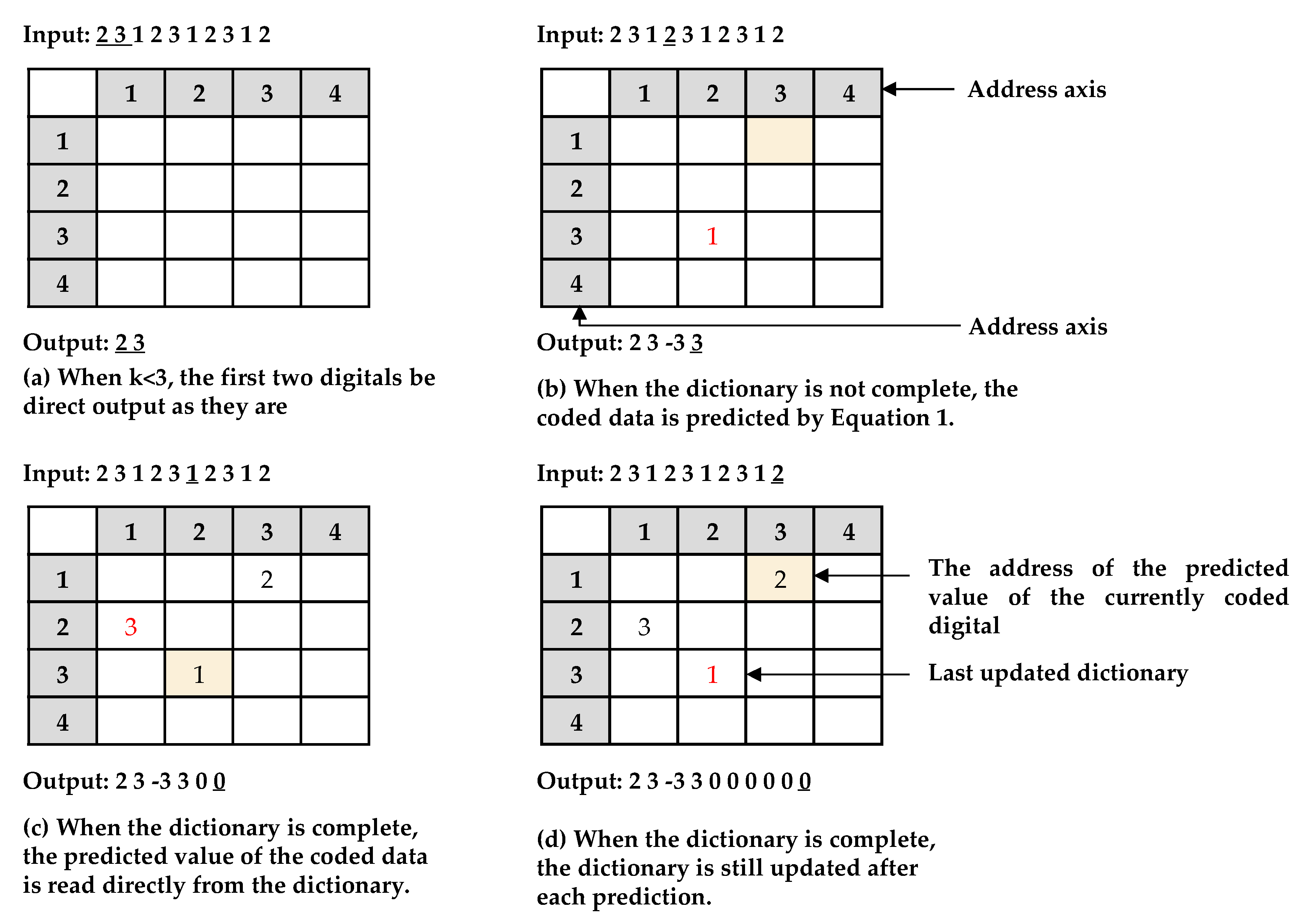
This example is Algorithm 1, which is shown in Figure 3. Assume that the input period data stream for the encoder is ‘2 3 1 2 3 1 2 3 1 2’. First, the first two digitals are read by the encoder. However, their first two adjacent digitals do not exist. Thus, they are directly output as they are (Figure 3a). When the dictionary is not complete, the dictionary D (3,1) is empty. The coded data is predicted as −1 by Equation (1). In Equation (1), a = −1, b = 2. Thus, the output value of the encoder is 3 (Figure 3b). When the dictionary is complete, the dictionary D (2,3) is not empty. The coded data is predicted as 1 by the dictionary. Thus, the output value of the encoder is 0 (Figure 3c). When the dictionary is complete, the dictionary is still updated after each prediction (Figure 3d). Finally, the data stream output by the encoder is ‘2 3 −3 3 0 0 0 0 0 0’.

2.2. Decoding Algorithm Introduction

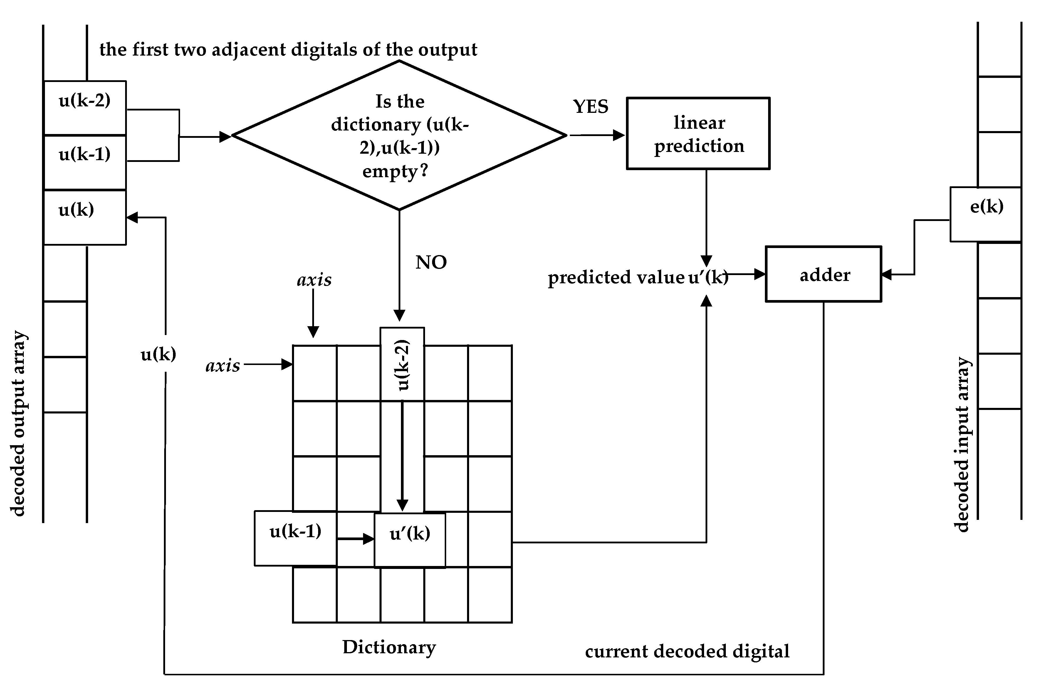
As shown in Figure 4, the decoding process is very similar to the coding process, it is assumed that a sequence $\left\{e(k)\right\}$ ($k$ = 1, 2, …, n) is given. Each symbol $e(k)$ belongs to a finite digital. The sequence $u(k)$ is the output of the decoding process.

First, the two-dimensional dictionary $H$ is created, whose size is the same as the dictionary $D$ of the coding process. The decoding output $u(k)$ of $e(k)$ is stored in the dictionary. The position of the digital $u(k)$ in the dictionary is the two-dimensional coordinate formed by the first two adjacent digitals $u(k-2)$ and $u(k-1)$. When the current decoded digital $e(k)$ is decoded, the predicted value $u^{\prime }(k)$ of the decoded digital is read in the dictionary with the address coordinate ($u(k-2)$, $u(k-1)$) of the first two adjacent digitals $u(k)$. Then the digital $e(k)$ to be decoded and the predicted value $u^{\prime }(k)$ are added to get a signal $u(k)=e(k)+u^{\prime }(k)$, which is the decoded output signal. When the decoding process ends, the adaptive dictionary is still discarded.

For the decoding process, this method has two special cases, as follows:

(1)

The first two digitals $e(1)$, $e(2)$ in the input array $\left\{e(k)\right\}$ to be decoded do not have the first two adjacent digitals. Therefore, the first two digitals cannot be decoded, and they need to be directly output as they are.

(2)

In the early stage of the decoding process, because the dictionary $H$ is not complete, there may not be predicted values in the dictionary. According to the first two adjacent digitals of the decoded output $u(k)$, Equation (2) can be used as the predicted value of the current digital to be encoded.

$$u^{\prime }(k)=a*u(k-2)+b*u(k-1),$$

(2)

where $u^{\prime }(k)$ is the predicted value of the current digital to be decoded, $u(k-1)$ and $u(k-2)$ are the first two adjacent digitals of the output of the current decoded digital. $a$ and $b$ are constant prediction coefficients, which are the same as the prediction Equation (1) coefficient in the coding process.

Algorithm 2 is the step of decoding algorithm, which works as follows:

Algorithm 2 steps of decoding algorithm

Input: decoded input {e(k)} Output: decoded output {u(k)}

Initialize- dictionary H

Initialize- address index k← 0

while k<=n                        %n is the length of input array{s(k)}

do k← k+1

if k<3

then u(k) ← e(k)

elseif H(u(k−2),u(k-1)) = NULL

then u’(k) ← a*u(k−2)+b*u(k−1)

else u’(k) ← H(u(k−2),u(k−1))

u(k) ← e(k)+u’(k)

H(u(k−2),u(k−1)) ← u(k)

end

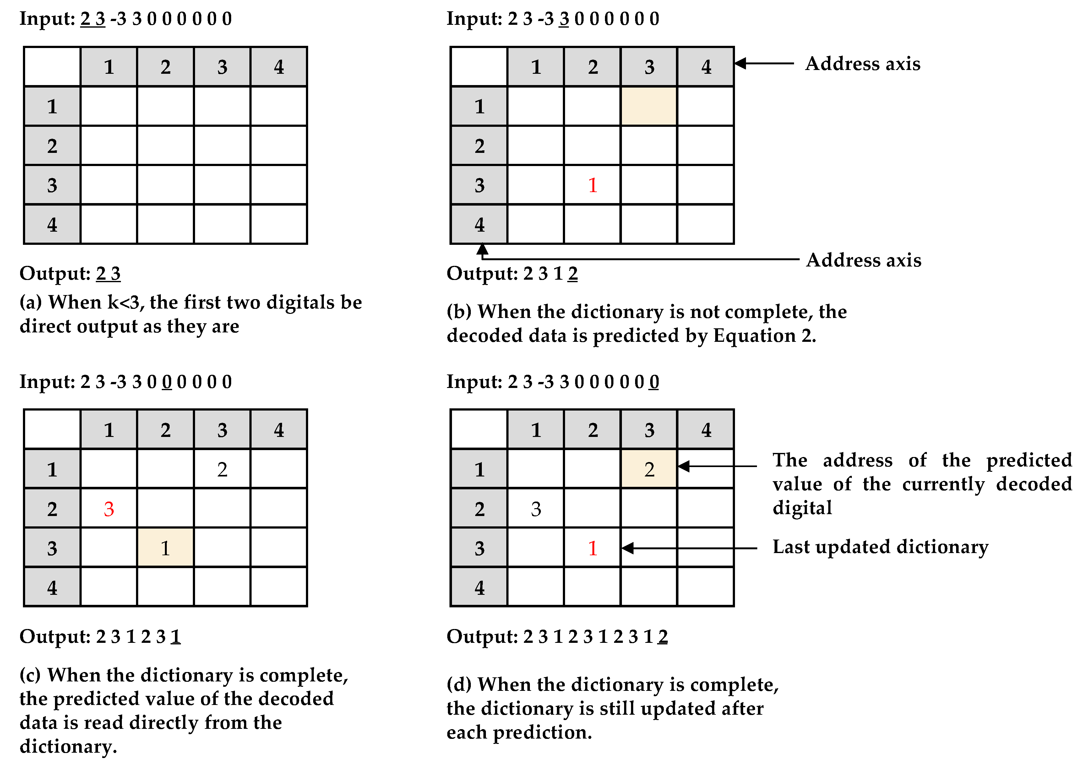
The example is Algorithm 2, which is shown in Figure 5. Assume that the input data stream for the decoder is ‘2 3 −3 3 0 0 0 0 0 0’. First, the first two digitals are read by the decoder. However, their first two adjacent digitals do not exist. Thus, they are directly output as they are (Figure 5a). When the dictionary is not complete, the dictionary H (3,1) is empty. The decoded data is predicted as −1 by Equation (2). In the Equation (2), a = −1, b = 2. Thus, the output value of the decoder is 2 (Figure 5b). When the dictionary is complete, the dictionary H (2,3) is not empty. The decoded data is predicted as 1 by the dictionary. Thus, the output value of the decoder is 1 (Figure 5c). When the dictionary is complete, the dictionary is still updated after each prediction (Figure 5d). Finally, the data stream output by the decoder is ‘2 3 1 2 3 1 2 3 1 2’.

3. Experiment and Result Analysis

3.1. Experiment

In the experiment, we use MATLAB2014b as an algorithm verification tool. Our process of compressing the signal is shown in Figure 6.

The lossless compression system does not include ‘data quantization’, which is a step of a lossy compression system. First, the test signal is processed by DC level shifting. Then, the transform coding or the predictive coding is used to process the signal. Finally, LZW is used to further compress the signal.

The calculation formula of DC level shifting is

$$y=x-x_{\min },$$

(3)

where $x$ is compressed data and $x_{\min }$ is the minimum value of the compressed data.

The experiment contains a total of three sets of data:

(1)

The first set of data is a periodic signal that changes period and amplitude with time to verify the feasibility of a lossless compression system.

(2)

The second set of data is a periodic signal with a period T = 200 and a signal length of L = 10 K. It is used to verify the effect of block size on compression efficiency. The formula of the signal is

$$y=80z+50\sin (\frac{2\pi }{50}x)+10\sin (\frac{2\pi }{20}x),$$

(4)

$$z=\{\begin{array}{cc}\frac{8}{9}(x-200*n)\hfill & \hfill 200n\le x<200n+180\\ -8(x-200*(n+1))\hfill & \hfill 200n+180\le x<200n+200\end{array} ,$$

(5)

where $n$ = 0, 1, …, 50.

(3)

The last set of data we selected is 10 different periodic signals, whose periods and amplitudes are different. Because the wavelet basis function has rich frequency domain information, we perform periodic extension of the wavelet basis function to obtain the above-mentioned 10 different sets of periodic signals. The detailed information of these 10 sets of periodic signals is shown in

Table 1. Experimental signal information.

Wavelet	Period	Length	Digital Width (Bit)
bior2.4	320	102.4 K	12
coif3	272	74 K	12
db4	224	50 K	12
dmey	200	40 K	12
haar	256	65.5 K	12
mexihat	256	65.5 K	12
meyer	256	65.5 K	12
morlet	256	65.5 K	12
rbio2.4	288	82.9 K	12
sym4	224	50 K	12

.

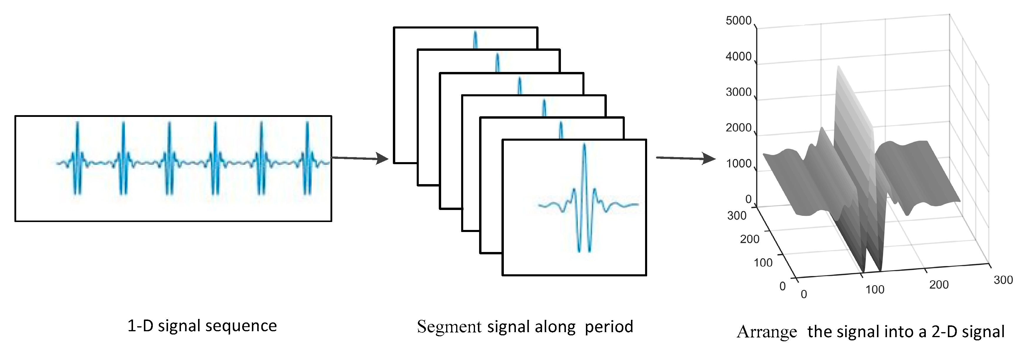
In [10,11], the authors studied the data compression algorithm based on the two-dimensional lifting format wavelet transform (2-D LWT) and two-dimensional discrete cosine transform (2-D DCT) in order to improve the data compression ratio and the efficiency of the compression algorithm. The basic idea is to first convert the periodic signal to be compressed from one-dimensional space to two-dimensional space, and then perform two-dimensional wavelet decomposition and two-dimensional discrete cosine transform, which can improve compression efficiency. The process of two-dimensional expression of one-dimensional data is as follows:

(1)

Segment the one-dimensional periodic signal along the period of the signal.

(2)

Arrange the cut signal into a two-dimensional signal.

In Figure 7, the process of two-dimension expression of one-dimension data is shown.

In the experiment, we chose several methods that currently have a good compression effect on periodic signals. They are two-dimensional discrete cosine transform (2-D DCT) [10], two-dimensional lifting wavelet transform (2-D LWT) [11] and differential pulse code modulation (DPCM) [13]. In addition, we used LZW to further compress the encoded output.

The workflow of these three methods is as follows:

In reference [10], 2-D DCT works as follows:

(1)

Segment 1-D signal along with multiples of the signal’s period.

(2)

Arrange the signal into a 2-D signal.

(3)

Divide the 2-D signal into 8×8 matrix blocks.

(4)

Perform 2D discrete cosine transform on 8×8 matrix blocks.

(5)

Quantize the transformed output.

In reference [11], 2-D LWT works as follows:

(1)

Segment 1-D signal along with multiples of the signal’s period.

(2)

Arrange the signal into a 2-D signal.

(3)

Perform 3-layer lifting wavelet transform on 2-D signal.

(4)

Quantize the transformed output.

DPCM works as follows:

(1)

The formula for predicting the actual value $x(k)$ is

$$x^{\prime }(k)={\displaystyle \sum _{i=1}^{N}a(i)x(k-i)},$$

(6)

(2)

The calculation formula of the output result signal is

$$e(k)=x(k)-x^{\prime }(k),$$

(7)

where $x^{\prime }(k)$ is the predicted value of the encoded number $x(k)$, and $a(i)$ is the prediction coefficient.

3.2. Experimental Evaluation Index

In the experiment, the compression ratio (CR) and information entropy were selected as the evaluation index. In addition, the peak signal to noise ratio (PSNR) is an objective standard for evaluating data compression.

The entropy feature is a measure of the uncertainty of a random variable [21]. The calculation formula of the average information entropy is

$$H(X)=-{\displaystyle \sum _{i=1}^{n}p(x(i)){\log }_2}p(x(i)),$$

(8)

where $X$ is the source, $x(i)$ is the character in the source, $p(x(i))$ is the probability that the character $x(i)$ appears in the source $X$, and the unit of $H(X)$ is bit/sign.

Equation (8) is the required sequence $\left\{x(i)\right\}$ as a discrete memoryless source. The method proposed in this paper is a prediction method, whose output is the prediction errors. The prediction error sequences are independent of each other, so it is memoryless. The amount of information in the predicted output sequence can be measured by the average information entropy, which can reflect the compressibility of the sequence.

The calculation formula of PSNR is:

$$PSNR=10•{\log }_{10}\left(\frac{MA{X}^2}{\frac{1}{L}{{\displaystyle \sum _{i=1}^L\left[x(i)-x^{\prime }(i)\right]}}^2}\right),$$

(9)

where $x$ is the original signal, $x^{\prime }$ is the signal after adding noise, $L$ is the length of the signal, $MAX$ is the maximum value of the signal, and PSNR is measured in dB.

The calculation formula for the compression ratio is:

$$M=\frac{S_{in}}{S_{out}},$$

(10)

where $S_{in}$ is the byte size before data compression, and $S_{out}$ is the byte size after data compression.

3.3. Result Analysis

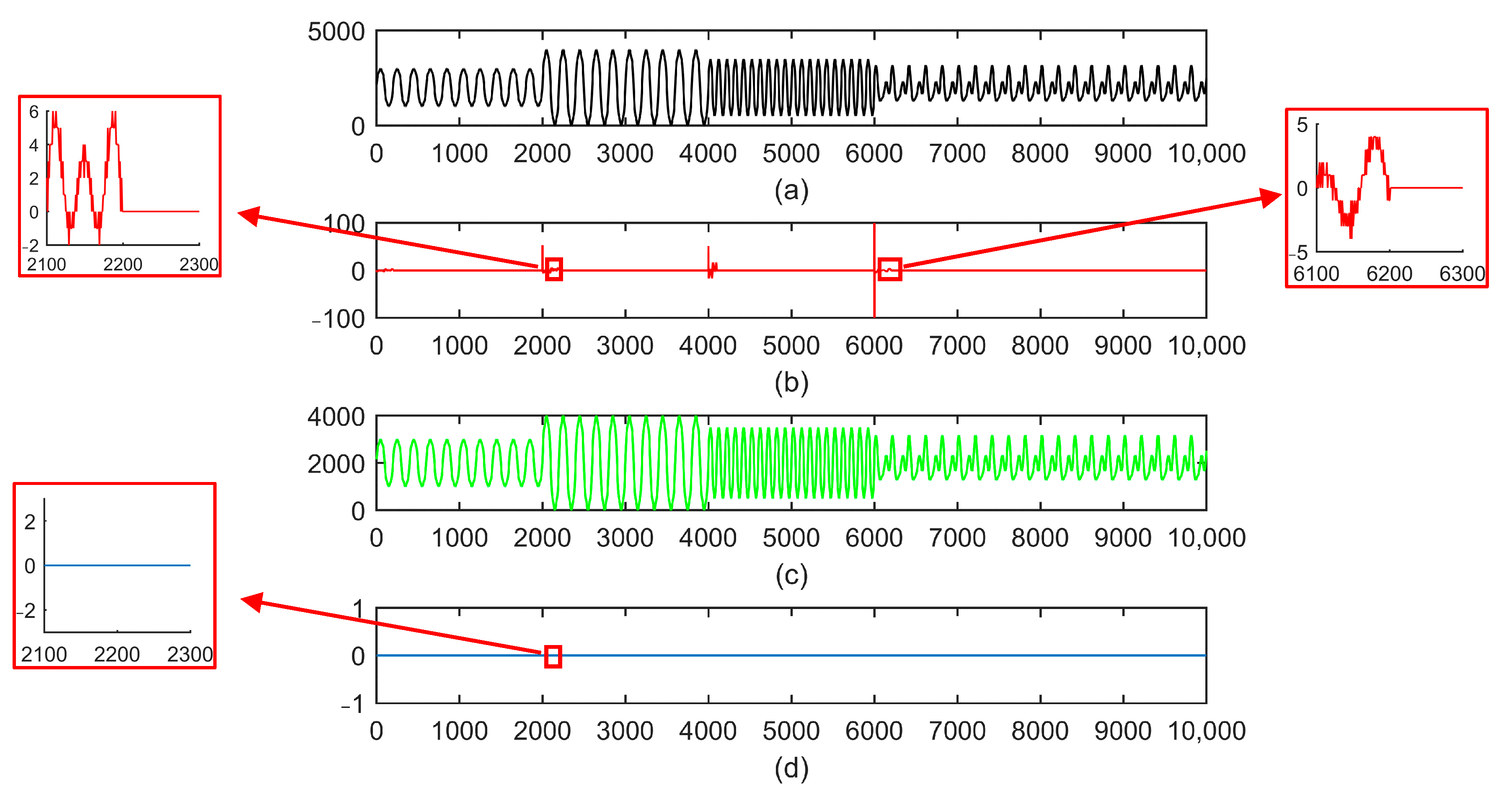
In order to verify the efficiency and adaptability of the method proposed in this paper, we used the method to predict and code the periodic signal, which has a varying period and amplitude.

Figure 8 verifies the efficiency and adaptability of the method proposed in this paper. We observed that the amplitude and period of the periodic signal change, which has little effect on the prediction accuracy of this method. This effect only occurs in the first period of amplitude and period changes. In addition, the output of the coding has a strong “energy concentration” characteristic, which has many 0 values. Furthermore, the method proposed in this paper is a lossless compression algorithm.

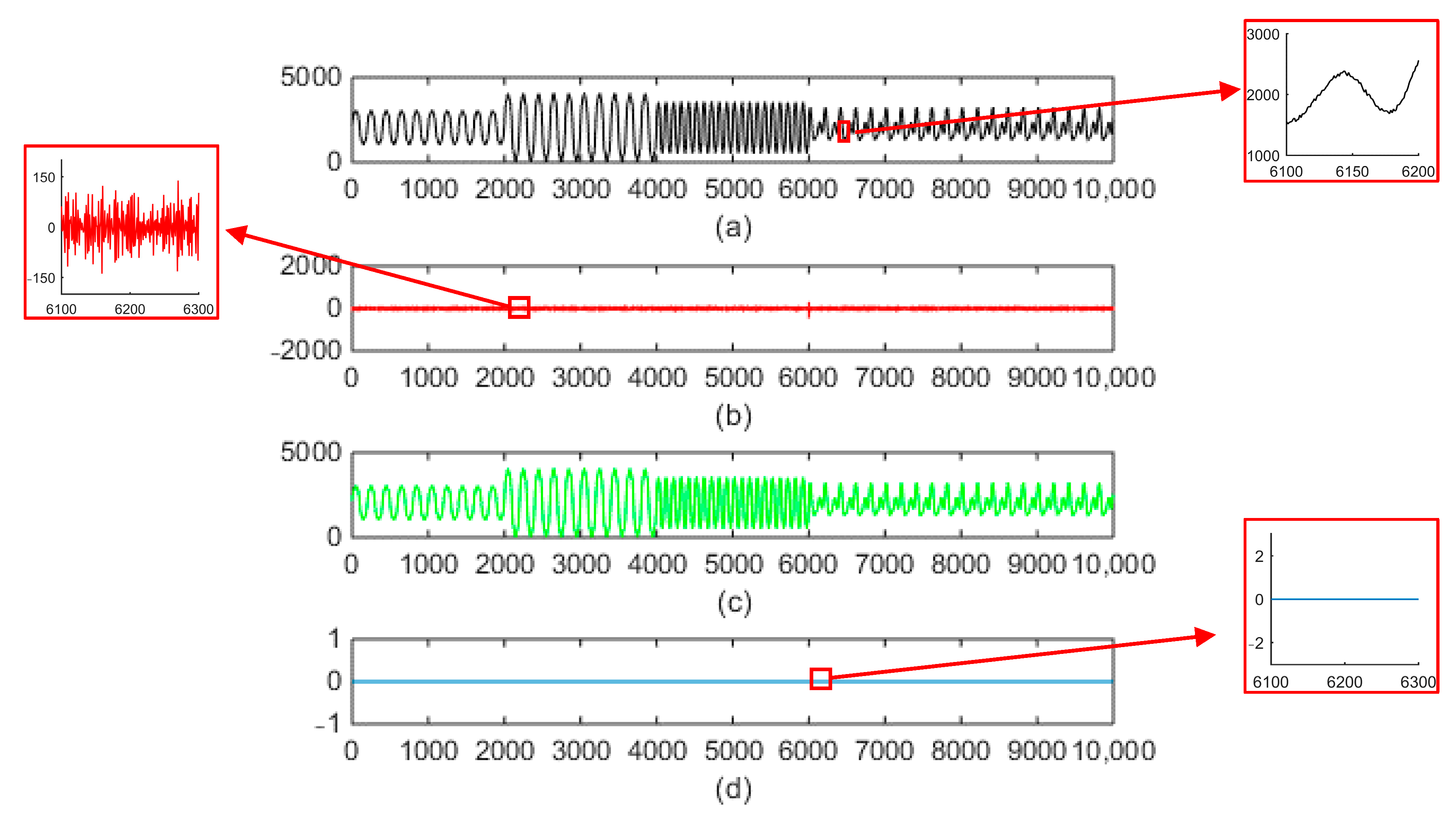
Next, the original signal in Figure 8 was the added noise, whose signal to noise ratio is 34.2 dB. In Figure 9, the prediction effect of this algorithm on the noise-added periodic signal, whose prediction effect is worse than the prediction effect in the Figure 8, is shown. This is because the method proposed in this paper is a lossless compression algorithm. We added the noise to the periodic signal, and the amplitude of the signal is random within a certain range. It is difficult for the prediction model to use context information to accurately predict the amplitude of the signal, so the output prediction residuals fluctuate within a small range. Therefore, the signal in Figure 9 is also the next in-depth research direction of this algorithm.

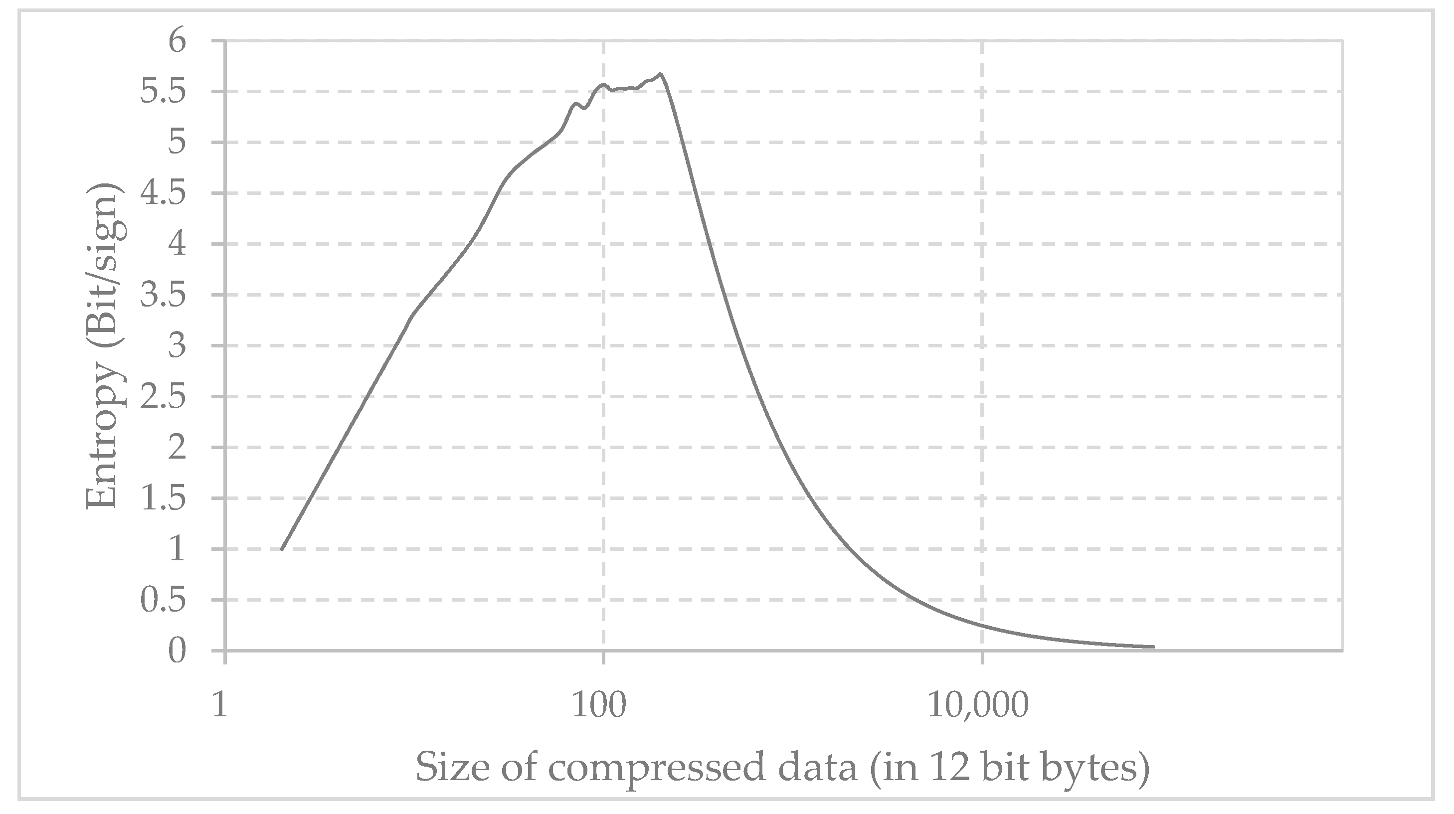
Then, the period signal with period T = 200 is selected. The signal was cut to different sizes (L = 1, 2, …, 10 K), which were coded by the method proposed in this paper. The entropy of the coding output were calculated by Equation (8).

By comparing the results in Figure 10, we can know that the larger the compressed data size, the better the predictive coding effect of this method. In addition, when the size of the compressed data is large enough, the information entropy no longer decreases, and the information entropy at this time reaches the limit.

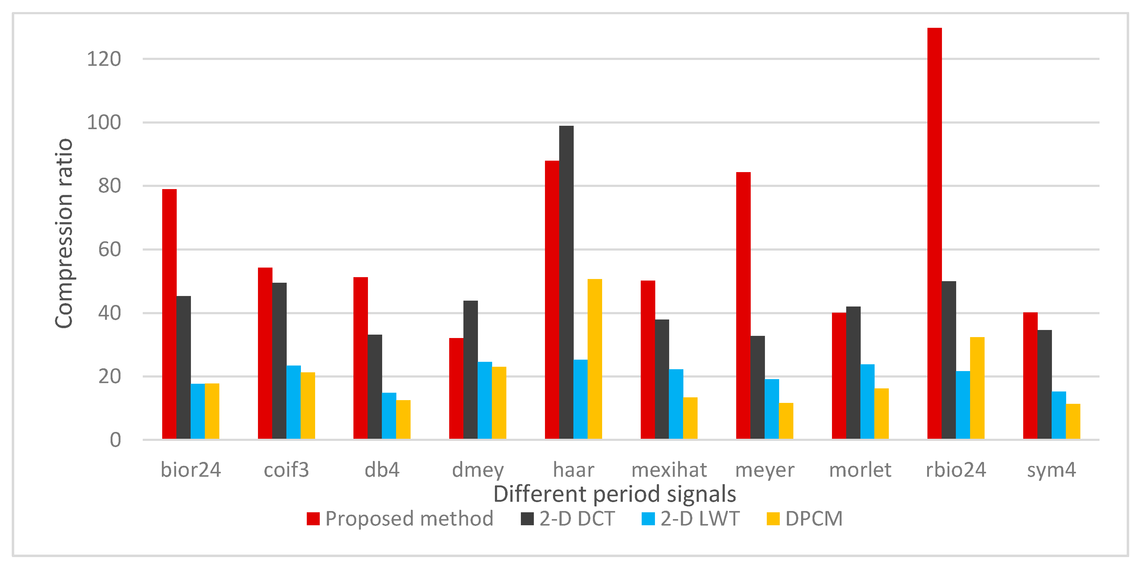
Finally, we selected 10 sets of sample signals that have different periods and amplitudes. The different methods, including the methods of this paper, 2-D DCT, 2-D LWT, and DPCM were selected to code 10 sets of periodic signals. In addition, LZW was used to further compress the signal.

By comparing the results in Figure 11 and

Table 2. Comparison of the compression ratio of the methods proposed in this paper with 2-D DCT, 2-D LWT, and DPCM.

Coding Methods	CRmean	CRmin	CRmax	PSNR (dB)
Proposed method	64.90	32.11	129.77	-
2-D DCT	46.78	32.72	98.92	63.77
2-D LWT	20.78	14.87	25.22	56.07
DPCM	21.00	11.31	50.63	-

$CRmean$ is the average of the compression ratio of 10 sets of data value, $CR\min$ is the minimum value of 10 sets of data compression ratio, $CR\max$ is the maximum value of 10 sets of data compression ratio. In addition, the encoded output results of 2-D DCT and 2-DLWT are quantized, so they belong to lossy compression. We calculated the compression ratio by Equation (10). $PSNR$ is the peak signal to noise ratio of the output signal. $PSNR$ is the average of the peak signal to noise ratio of 10 sets of data value. When the value of $PSNR$ is “-”, it represents lossless compression. We calculated $PSNR$ by Equation (9).

, we can see that the coding effect of this paper’s method on periodic signals is much better than the other three methods. When the coding output of the method proposed in this paper is compressed by LZW, the compression ratio is much higher than the other three methods. Furthermore, the method proposed in this paper belongs to lossless compression. When the signal is compressed by the method, the signal information will not be lost.

The time complexity of our proposed method, DPCM, 2-D DCT, and 2-D LWT are presented in

Table 3. Time complexity of different methods.

Coding Methods	Time Complexity
Proposed method	O(n)
DPCM	O(n)
2-D DCT	O(n2)
2-D LWT	O(n)

. The time complexity of our proposed method is the same as that of DPCM and 2-D LWT, and is simpler than that of 2-D DCT.

4. Conclusions

In this paper, aiming at the problem of periodic signal compression, a new adaptive coding method was proposed. Its coding output is compressed by LZW. Experimentally, we can verify that the advantages of our proposed method are:

(1)

The results obtained proved that the output of the coding has a strong “energy concentration” characteristic, which has many 0 values.

(2)

Our proposed method has a strong adaptive ability, the amplitude and period of the periodic signal change, which has little effect on the prediction accuracy of this method.

(3)

By comparing with 2-D DCT, 2-D LWT, and DPCM, our proposed method is more effective in compressing periodic signals. It is combined with LZW to compress the periodic signal and has a high compression ratio.

(4)

The complexity of the method proposed in this paper, which is $O(n)$, is low.

References

- Tripathi, R.P.; Mishra, G.R. Study of various data compression techniques used in lossless compression of ECG signals. In Proceedings of the 2017 International Conference on Computing, Communication and Automation (ICCCA), Greater Noida, India, 5–6 May 2017; pp. 1093–1097. [Google Scholar] [CrossRef]
- Gao, X. On the improved correlative prediction scheme for aliased electrocardiogram (ECG) data compression. In Proceedings of the 2012 Annual International Conference of the IEEE Engineering in Medicine and Biology Society, San Diego, CA, USA, 28 August–1 September 2012; pp. 6180–6183. [Google Scholar] [CrossRef]
- Guo, L.; Zhou, D.; Goto, S. Lossless embedded compression using multi-mode DPCM & averaging prediction for HEVC-like video codec. In Proceedings of the 21st European Signal Processing Conference (EUSIPCO 2013), Marrakech, Morocco, 9–13 September 2013; pp. 1–5. [Google Scholar]
- Arshad, R.; Saleem, A.; Khan, D. Performance comparison of Huffman Coding and Double Huffman Coding. In Proceedings of the 2016 Sixth International Conference on Innovative Computing Technology (INTECH), Dublin, Ireland, 24–26 August 2016; pp. 361–364. [Google Scholar] [CrossRef]
- Huang, J.-Y.; Liang, Y.-C.; Huang, Y.-M. Secure integer arithmetic coding with adjustable interval size. In Proceedings of the 2013 19th Asia-Pacific Conference on Communications (APCC), Denpasar, India, 29–31 August 2013; pp. 683–687. [Google Scholar] [CrossRef]
- Khosravifard, M.; Narimani, H.; Gulliver, T.A. A Simple Recursive Shannon Code. IEEE Trans. Commun. 2012, 60, 295–299. [Google Scholar] [CrossRef]
- Hou, A.-L.; Yuan, F.; Ying, G. QR code image detection using run-length coding. In Proceedings of the 2011 International Conference on Computer Science and Network Technology, Harbin, China, 24–26 December 2011; pp. 2130–2134. [Google Scholar] [CrossRef]
- Nishimoto, T.; Tabei, Y. LZRR: LZ77 Parsing with Right Reference. In Proceedings of the 2019 Data Compression Conference (DCC), Snowbird, UT, USA, 26–29 March 2019; pp. 211–220. [Google Scholar] [CrossRef] [Green Version]
- Nandi, U.; Mandal, J.K. A Compression Technique Based on Optimality of LZW Code (OLZW). In Proceedings of the 2012 Third International Conference on Computer and Communication Technology, Allahabad, India, 23–25 November 2012; pp. 166–170. [Google Scholar] [CrossRef]
- An, Q.; Zhang, H.; Hu, Z.; Chen, Z. A Compression Approach of Power Quality Monitoring Data Based on Two-dimension DCT. In Proceedings of the 2011 Third International Conference on Measuring Technology and Mechatronics Automation, Shanghai, China, 6–7 January 2011; pp. 20–24. [Google Scholar]
- Zhang, R.; Yao, H.; Zhang, C. Compression method of power quality data based on wavelet transform. In Proceedings of the 2013 2nd International Conference on Measurement, Information and Control, Harbin, China, 16–18 August 2013; pp. 987–990. [Google Scholar]
- Tsai, T.; Tsai, F. Efficient Lossless Compression Scheme for Multi-channel ECG Signal. In Proceedings of the ICASSP 2019—2019 IEEE International Conference on Acoustics, Speech and Signal Processing (ICASSP), Brighton, UK, 12–17 May 2019; pp. 1289–1292. [Google Scholar]
- Alam, S.; Gupta, R. A DPCM based Electrocardiogram coder with thresholding for real time telemonitoring applications. In Proceedings of the 2014 International Conference on Communication and Signal Processing, Melmaruvathur, India, 3–5 April 2014; pp. 176–180. [Google Scholar]
- Liu, B.; Cao, A.; Kim, H. Unified Signal Compression Using Generative Adversarial Networks. In Proceedings of the ICASSP 2020—2020 IEEE International Conference on Acoustics, Speech and Signal Processing (ICASSP), Barcelona, Spain, 4–9 May 2020; pp. 3177–3181. [Google Scholar] [CrossRef] [Green Version]
- Wang, I.; Ding, J.; Hsu, H. Prediction techniques for wavelet based 1-D signal compression. In Proceedings of the 2017 Asia-Pacific Signal and Information Processing Association Annual Summit and Conference (APSIPA ASC), Kuala Lumpur, Malaysia, 12–15 December 2017; pp. 23–26. [Google Scholar] [CrossRef]
- Huang, F.; Qin, T.; Wang, L.; Wan, H.; Ren, J. An ECG Signal Prediction Method Based on ARIMA Model and DWT. In Proceedings of the 2019 IEEE 4th Advanced Information Technology, Electronic and Automation Control Conference (IAEAC), Chengdu, China, 20–22 December 2019; pp. 1298–1304. [Google Scholar] [CrossRef]
- Hikmawati, F.; Setyowati, E.; Salehah, N.A.; Choiruddin, A. A novel hybrid GSTARX-RNN model for forecasting space-time data with calendar variation effect. J. Phys. Conf. Ser. Kota Ambon Indones. 2020, 1463, 012037. [Google Scholar] [CrossRef]
- Jacquet, P.; Szpankowski, W.; Apostol, I. A universal pattern matching predictor for mixing sources. In Proceedings of the IEEE International Symposium on Information Theory, Lausanne, Switzerland, 30 June–5 July 2002; p. 150. [Google Scholar] [CrossRef]
- Feder, M.; Merhav, N.; Gutman, M. Universal prediction of individual sequences. IEEE Trans. Inf. Theory 1992, 38, 1258–1270. [Google Scholar] [CrossRef] [Green Version]
- Cleary, J.G.; Witten, I.H. Data compression using adaptive coding and partial string matching. IEEE Trans. Commun. 1984, 32, 396–402. [Google Scholar] [CrossRef] [Green Version]
- Cover, T.M.; Thomas, J.A. Elements of Information Theory; John Wiley & Sons: Hoboken, NJ, USA, 2012. [Google Scholar]
Figure 1.
Block diagram of data compression and decompression.
Figure 2.
Principle block diagram of the coding algorithm.
Figure 3.
Example of the predictive coding algorithm based on the adaptive dictionary.
Figure 4.
Principle block diagram of the decoding algorithm.
Figure 5.
Example of predictive decoding algorithm based on adaptive dictionary.
Figure 6.
The block diagram of a compression system.
Figure 7.
The process of two-dimensional expression of one-dimensional data.
Figure 8.
(a) Original signal (b) Coding output (c) Decoding output (d) Error between the decoding output and the original signal.
Figure 9.
(a) The signals containing additive noise (b) Coding output (c) Decoding output (d) Error between the decoding output result and the original signal.
Figure 10.
The effect of block size on compression efficiency.
Figure 11.
Comparison of the compression ratio of the signal compression by LZW.