Hybrid Malware Classification Method Using Segmentation-Based Fractal Texture Analysis and Deep Convolution Neural Network Features

 , , , and
Abstract
:1. Introduction
- The conversion of malware binaries into the grayscale image.
- Data augmentation performed on malware images to overcome the data imbalance within the malware datasets for robust feature extraction to enhance the classifier performance.
- An optimized multimodal feature representation to combine the segmentation-based fractal texture analysis (SFTA) features [15] and deep convolutional neural network (DCNN) features into a single feature vector to obtain a robust malware classification model.
2. Related Work
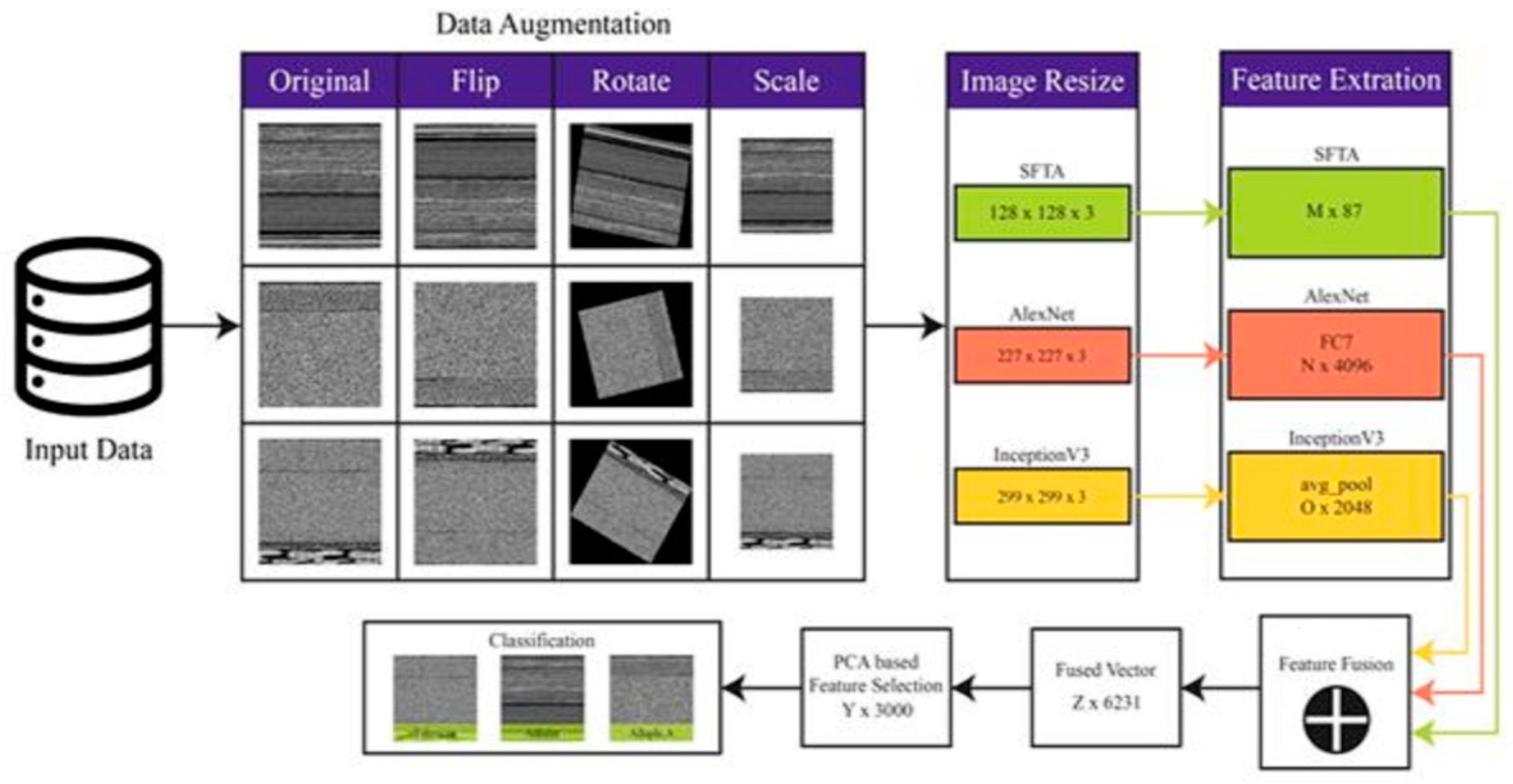
3. Methodology
3.1. Outline of Methodology
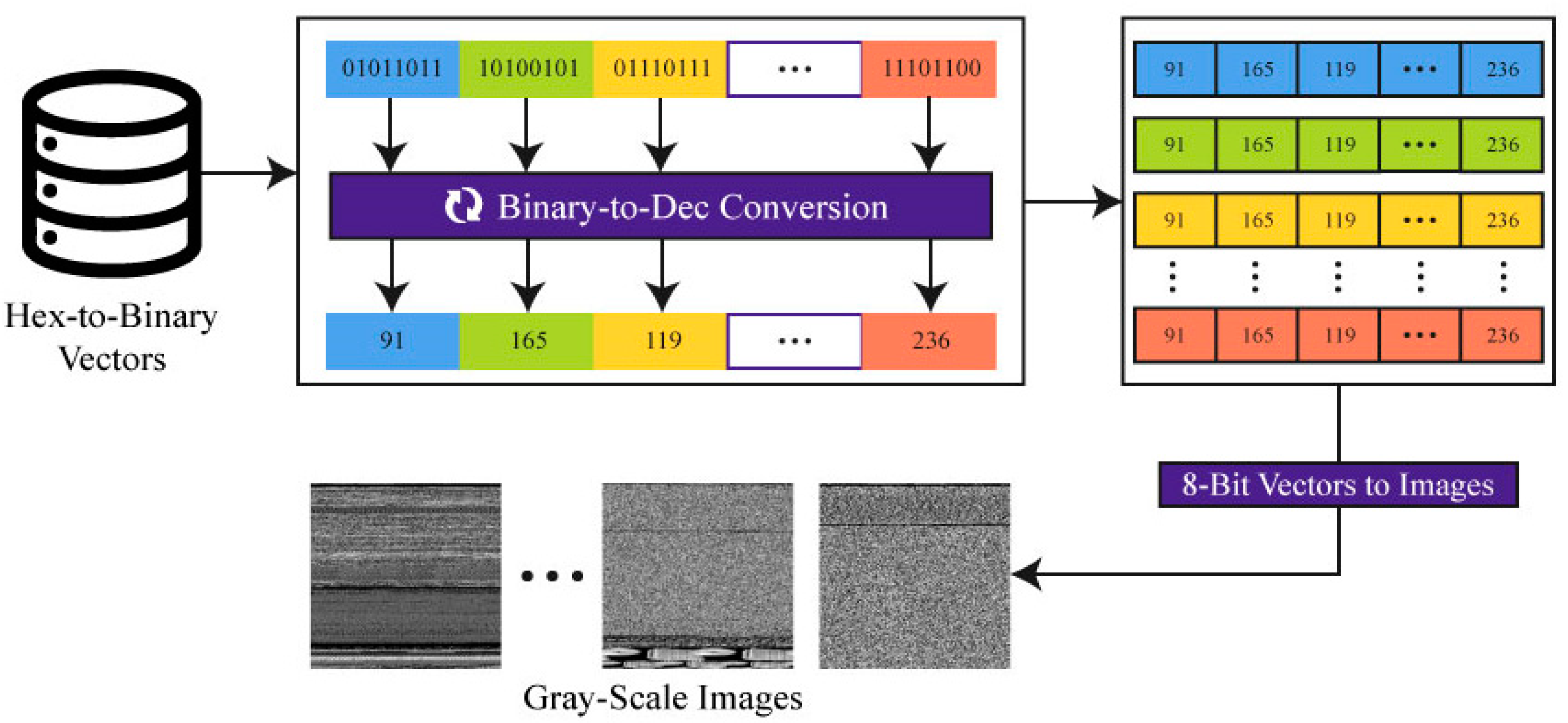
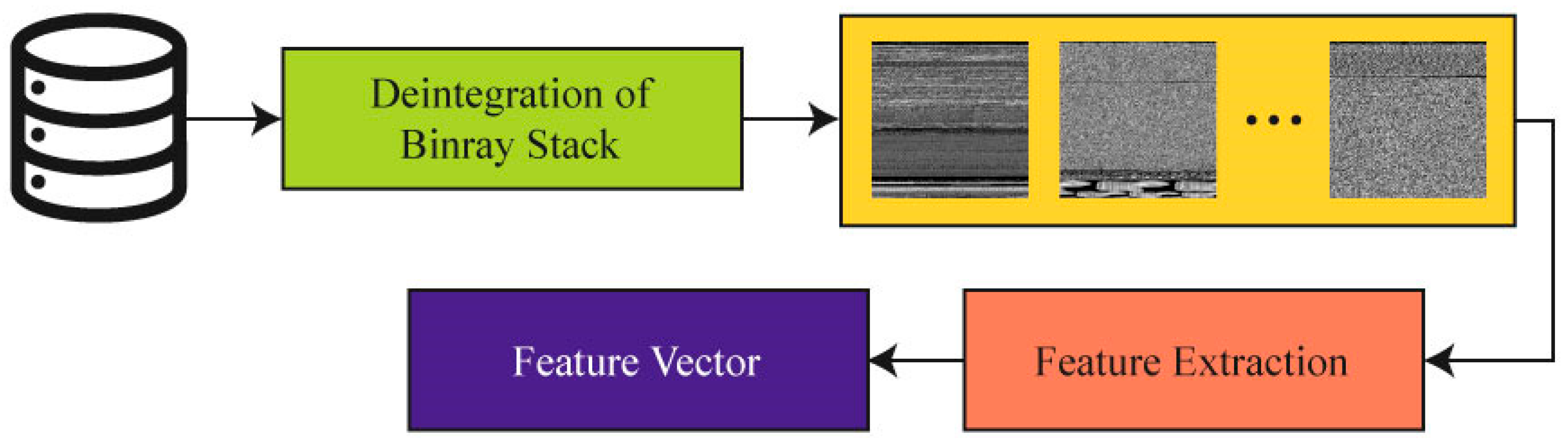
3.2. Visualization of Binary to a Grayscale Image
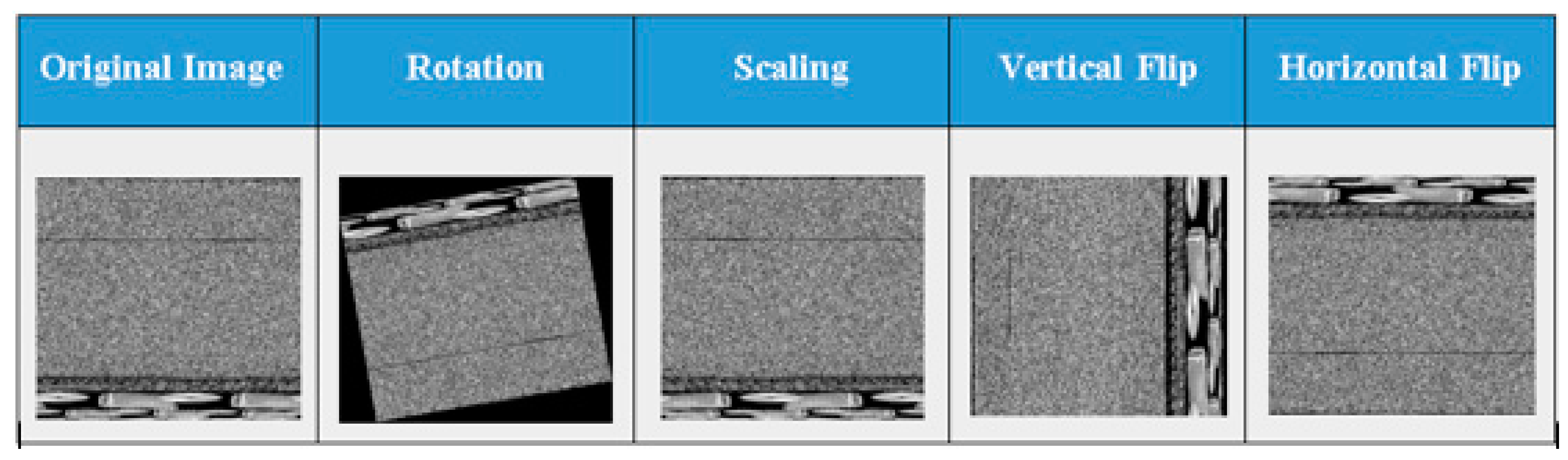
3.3. Image Augmentation
| Algorithm 1. Malware Image Augmentation |
| Input: Malware images , image flipping (Vertical and Horizontal) and rotation where is the rotation angle. Output: Rotation of malware image and flipped malware image . 1: for each Image do 2: for to 3: Angle of rotation to 4: end for 5: for 6: Flipping 7: end for 8: end for 9: return and |
3.4. Feature Extraction
3.4.1. Texture Feature (SFTA)
| Algorithm 2. SFTA Feature Extraction Algorithm |
| Require: Grayscale image and two thresholds and . Ensure: SFTA feature vector . 1: MultiLevelOtsus 2: 3: 4: 5: for do 6: Two Thresholds 7: Find Borders 8: Box Counting 9: MeanGrayLevel 10: Pixel Count 11: 12: end for 13: return |
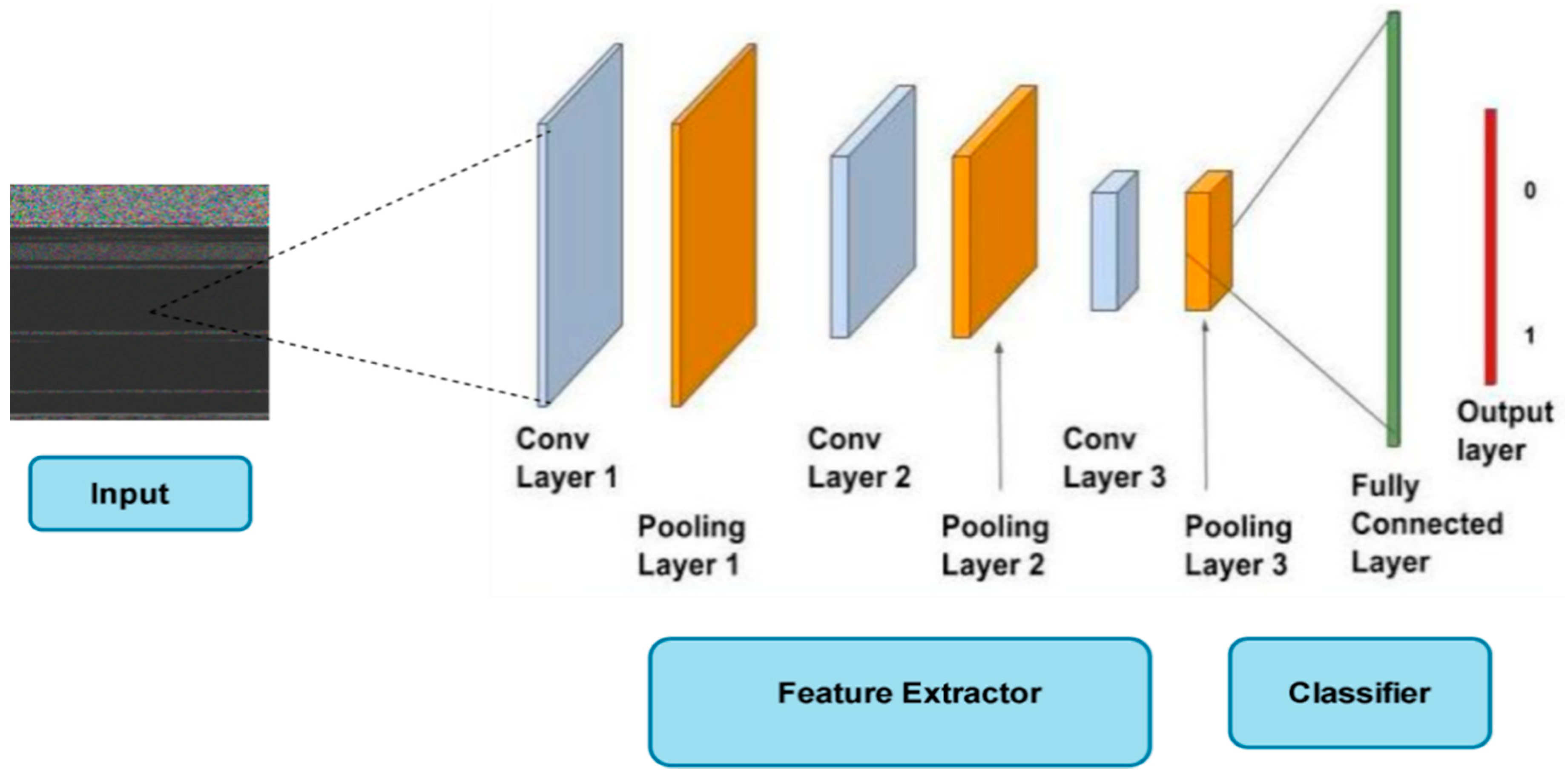
3.4.2. Deep Convolution Neural Network (DCNN)
3.4.3. DCNN Feature Extraction and Fusion
3.5. Feature Selection
4. Results and Analysis
4.1. Dataset
4.2. Settings
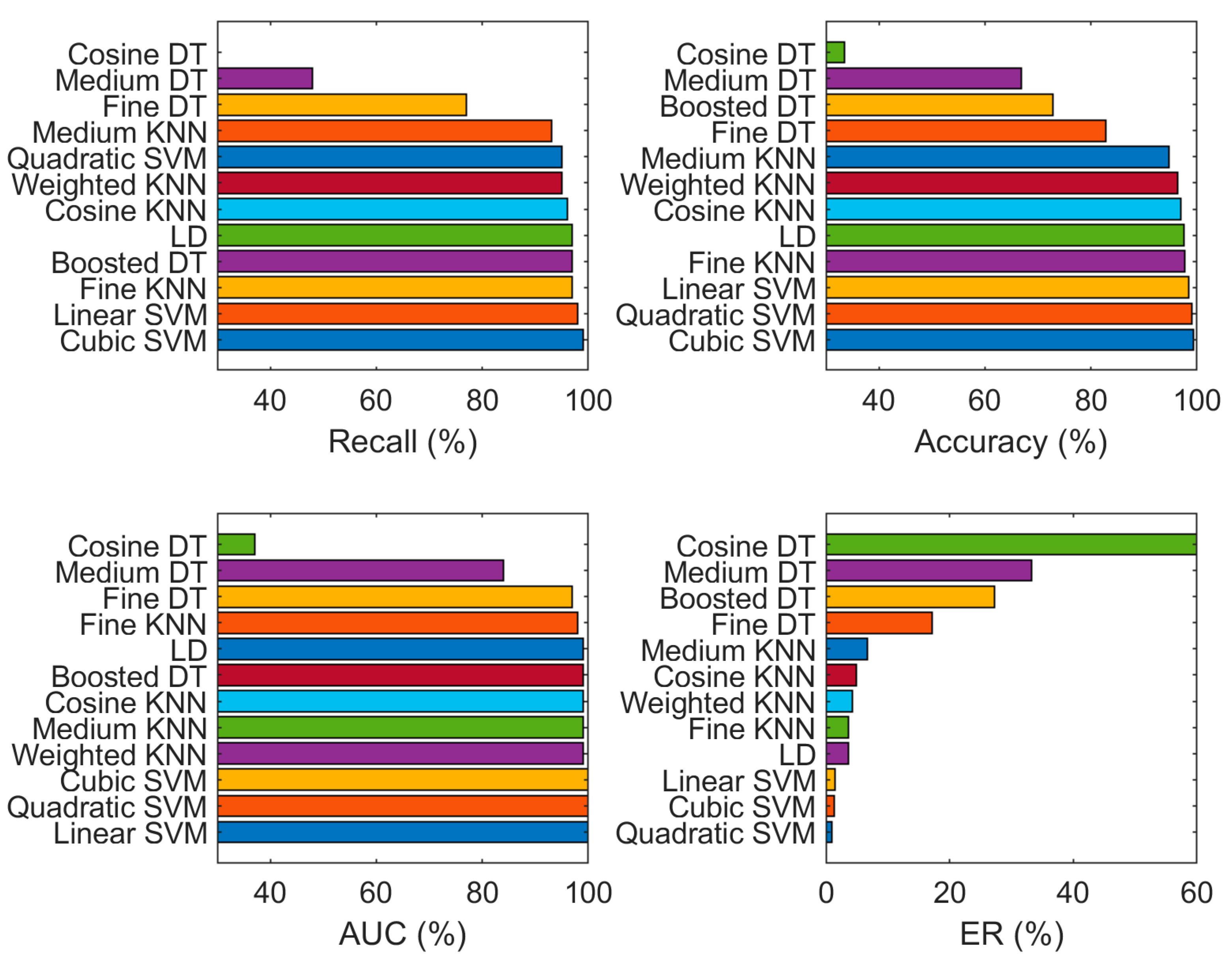
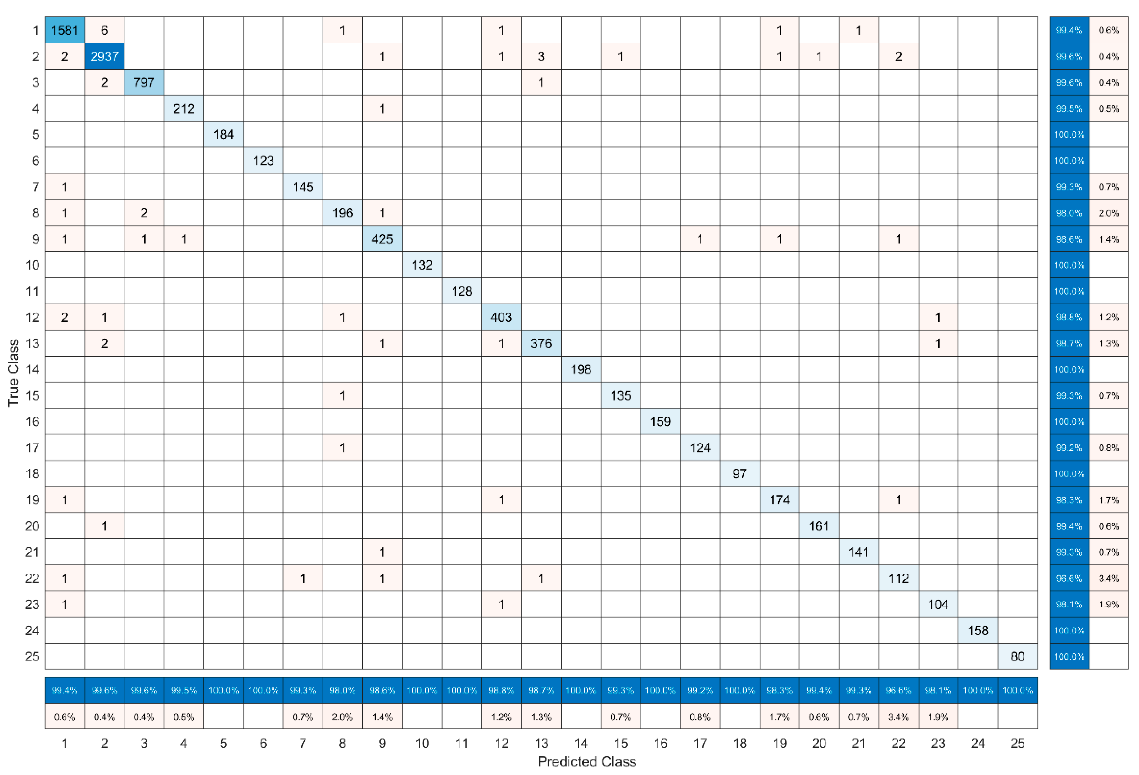
4.3. Results
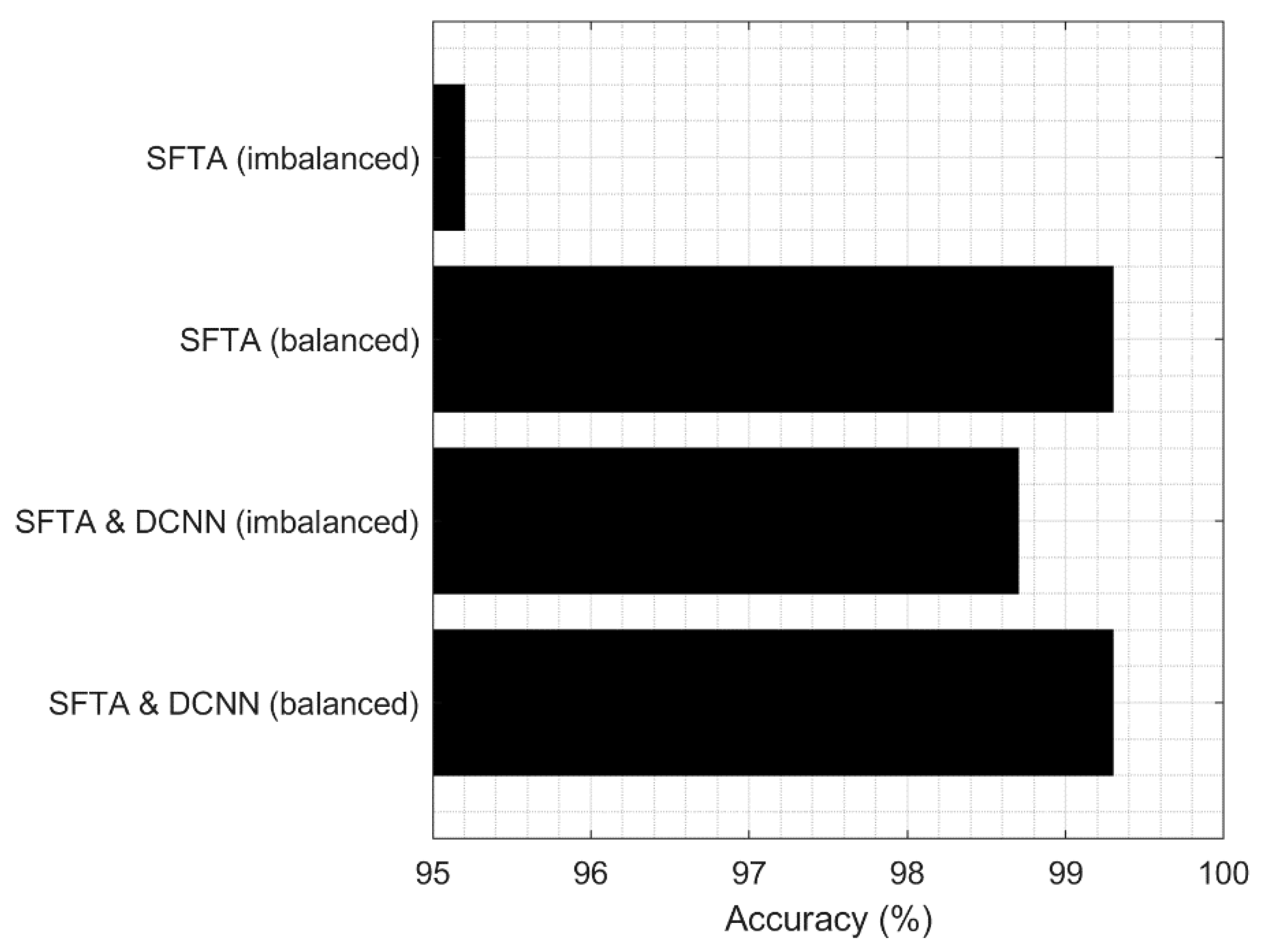
4.3.1. Experiment 1: With Imbalanced Data and SFTA Features without Feature Fusion and Feature Optimization
4.3.2. Experiment 2: With Balanced (Augmented) Data and SFTA Features
4.3.3. Experiment 3: With Imbalanced Data and Using Featured Obtained from a Pre-Trained Network Model
4.3.4. Experiment 4: With Balanced Data and Fusion of SFTA and Pre-Trained Network Features
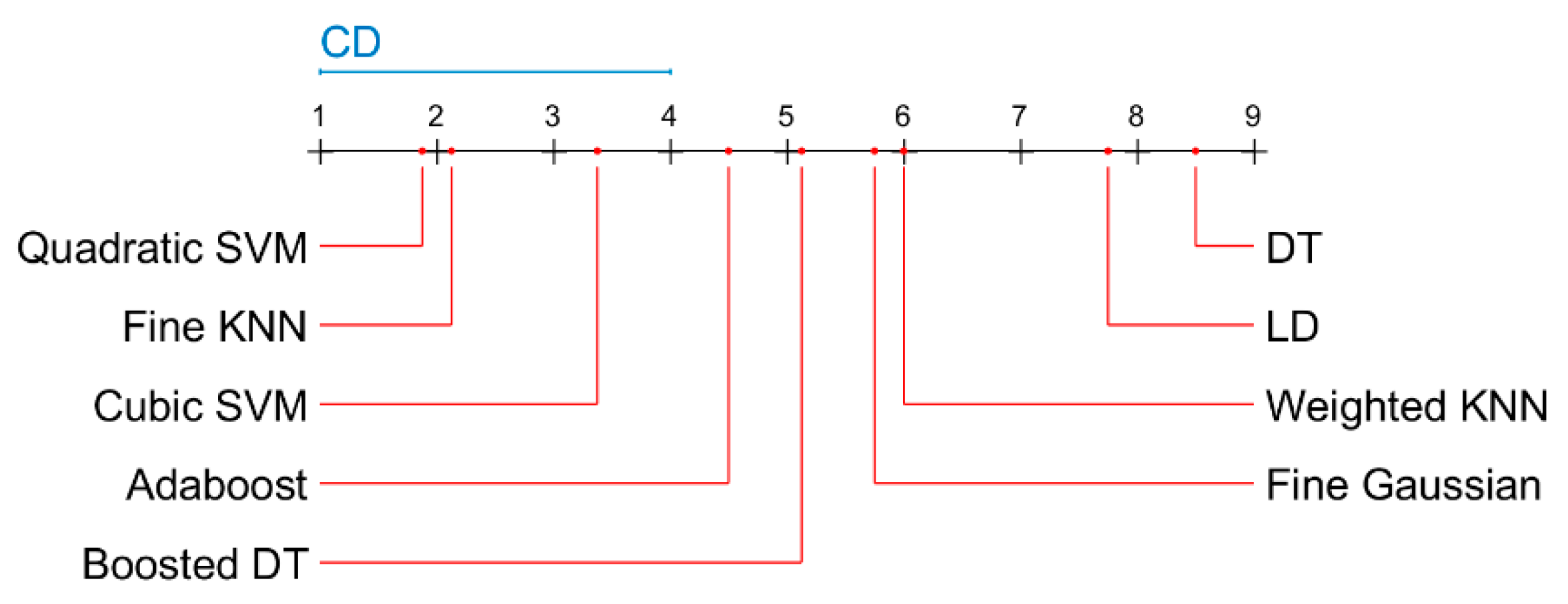
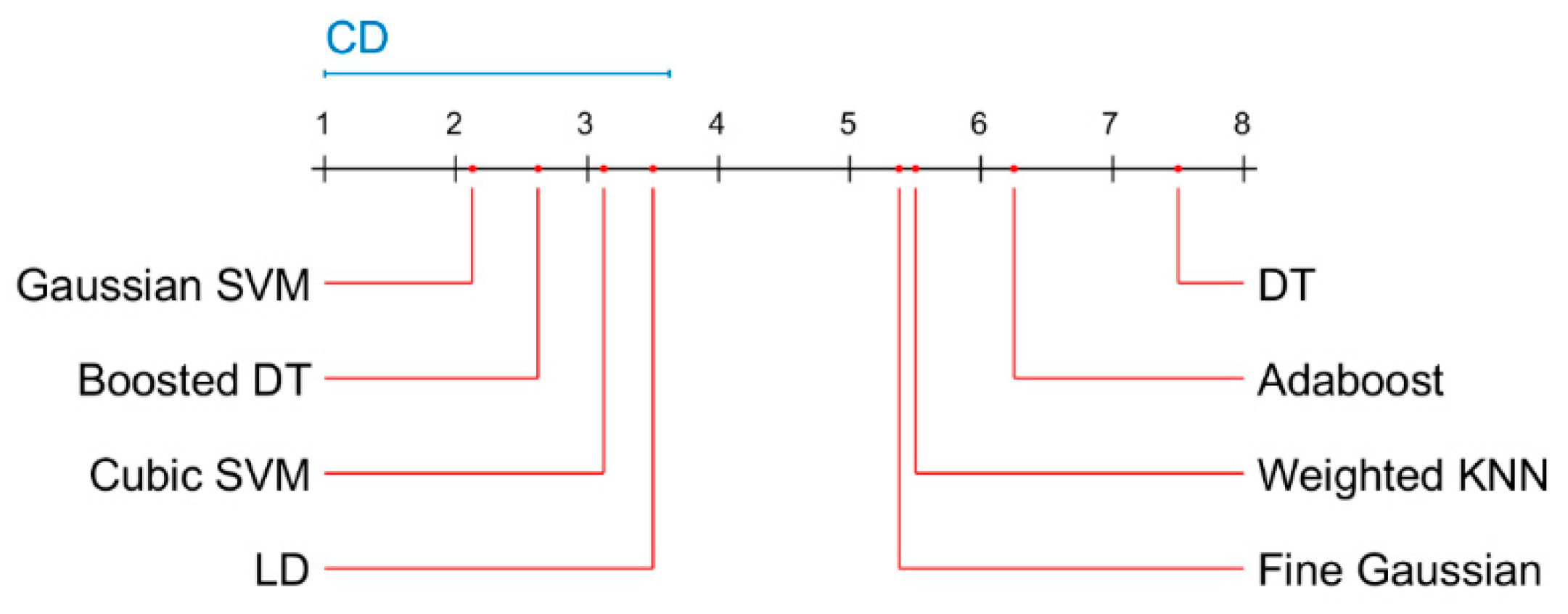
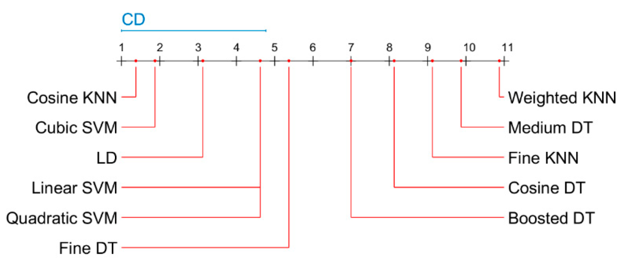
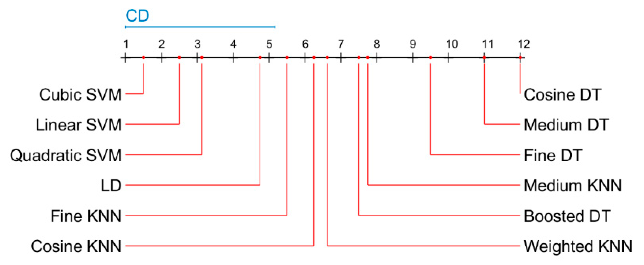
4.4. Statistical Analysis
4.5. Comparison of the Results of the Proposed Technique with Other Existing Methods
5. Conclusions
Author Contributions
Funding
Conflicts of Interest
References
- Symantec. Internet Security Threat Report (ISTR), Technical Report. 2019. Available online: https://www.symantec.com/content/dam/symantec/docs/reports/istr-24-2019-en.pdf (accessed on 1 June 2020).
- Alsoghyer, S.; Almomani, I. Ransomware Detection System for Android Applications. Electronics 2019, 8, 868. [Google Scholar] [CrossRef] [Green Version]
- Chun, S.-H. E-Commerce Liability and Security Breaches in Mobile Payment for e-Business Sustainability. Sustainability 2019, 11, 715. [Google Scholar] [CrossRef] [Green Version]
- Wangen, G. The Role of Malware in Reported Cyber Espionage: A Review of the Impact and Mechanism. Information 2015, 6, 183–211. [Google Scholar] [CrossRef] [Green Version]
- Subairu, S.O.; Alhassan, J.; Misra, S.; Abayomi-Alli, O.; Ahuja, R.; Damasevicius, R.; Maskeliunas, R. An Experimental Approach to Unravel Effects of Malware on System Network Interface. In Lecture Notes in Electrical Engineering; Springer: Singapore, 2019; pp. 225–235. [Google Scholar] [CrossRef]
- Odusami, M.; Abayomi-Alli, O.; Misra, S.; Shobayo, O.; Damasevicius, R.; Maskeliunas, R. Android Malware Detection: A Survey. In International Conference on Applied Informatics, ICAI, Proceedings of the Communications in Computer and Information Science, Bogotá, Colombia, 1–3 November 2018; Springer International Publishing: New York, NY, USA, 2018; Volume 942, pp. 255–266. [Google Scholar] [CrossRef]
- Vinayakumar, R.; Alazab, M.; Soman, K.P.; Poornachandran, P.; Venkatraman, S. Robust Intelligent Malware Detection Using Deep Learning. IEEE Access 2019, 7, 46717–46738. [Google Scholar] [CrossRef]
- Aslan, O.; Samet, R. A Comprehensive Review on Malware Detection Approaches. IEEE Access 2020, 8, 6249–6271. [Google Scholar] [CrossRef]
- Pan, S.J.; Yang, Q. A Survey on Transfer Learning. IEEE Trans. Knowl. Data Eng. 2010, 22, 1345–1359. [Google Scholar] [CrossRef]
- Kancherla, K.S.; Mukkamala, S. Image visualization based malware detection. In Proceedings of the 2013 IEEE Symposium on Computational Intelligence in Cyber Security (CICS), Singapore, 16–19 April 2013; pp. 40–44. [Google Scholar] [CrossRef]
- Vasan, D.; Alazab, M.; Wassan, S.; Naeem, H.; Safaei, B.; Zheng, Q. IMCFN: Image-based malware classification using fine-tuned convolutional neural network architecture. Comput. Netw. 2020, 171, 107138. [Google Scholar] [CrossRef]
- Cui, Z.; Xue, F.; Cai, X.; Cao, Y.; Wang, G.; Chen, J. Detection of Malicious Code Variants Based on Deep Learning. IEEE Trans. Ind. Inform. 2018, 14, 3187–3196. [Google Scholar] [CrossRef]
- Ye, Y.; Li, T.; Adjeroh, D.; Iyengar, S.S. A Survey on Malware Detection Using Data Mining Techniques. ACM Comput. Surv. 2017, 50, 1–40. [Google Scholar] [CrossRef]
- Kaur, H.; Pannu, H.S.; Malhi, A.K. A Systematic Review on Imbalanced Data Challenges in Machine Learning. ACM Comput. Surv. 2019, 52, 1–36. [Google Scholar] [CrossRef] [Green Version]
- Costa, A.F.; Humpire-Mamani, G.; Traina, A.J.M. An Efficient Algorithm for Fractal Analysis of Textures. In Proceedings of the 2012 25th SIBGRAPI Conference on Graphics, Patterns and Images, Ouro Preto, Brazil, 22–25 August 2012; pp. 39–46. [Google Scholar] [CrossRef]
- Khan, M.A.; Javed, K.; Khan, S.A.; Saba, T.; Habib, U.; Khan, J.A.; Abbasi, A.A. Human action recognition using fusion of multiview and deep features: An application to video surveillance. Multimed. Tools Appl. 2020, 1–27. [Google Scholar] [CrossRef]
- Arshad, H.; Khan, M.A.; Sharif, M.I.; Yasmin, M.; Tavares, J.M.R.S.; Zhang, Y.D.; Satapathy, S.C. A multilevel paradigm for deep convolutional neural network features selection with an application to human gait recognition. Expert Syst. 2020, e12541. [Google Scholar] [CrossRef]
- Mehmood, A.; Khan, M.A.; Sharif, M.; Khan, S.A.; Shaheen, M.; Saba, T.; Riaz, N.; Ashraf, I. Prosperous Human Gait Recognition: An end-to-end system based on pre-trained CNN features selection. Multimed. Tools Appl. 2020. [Google Scholar] [CrossRef]
- Rashid, M.; Khan, M.A.; Alhaisoni, M.; Wang, S.H.; Naqvi, S.R.; Rehman, A.; Saba, T. A Sustainable Deep Learning Framework for Object Recognition Using Multi-Layers Deep Features Fusion and Selection. Sustainability 2020, 12, 5037. [Google Scholar] [CrossRef]
- Hussain, N.; Khan, M.A.; Sharif, M.; Khan, S.A.; Albesher, A.A.; Saba, T.; Armaghan, A. A deep neural network and classical features based scheme for objects recognition: An application for machine inspection. Multimed Tools Appl. 2020. [Google Scholar] [CrossRef]
- Rauf, H.T.; Shoaib, U.; Lali, M.I.; Alhaisoni, M.; Irfan, M.N.; Khan, M.A. Particle Swarm Optimization WITH Probability Sequence for Global Optimization. IEEE Access 2020, 8, 110535–110549. [Google Scholar] [CrossRef]
- Khan, M.A.; Khan, M.A.; Ahmed, F.; Mittal, M.; Goyal, L.M.; Jude Hemanth, D.; Satapathy, S.C. Gastrointestinal diseases segmentation and classification based on duo-deep architectures. Pattern Recognit. Lett. 2020, 131, 193–204. [Google Scholar] [CrossRef]
- Sharif, M.I.; Li, J.P.; Khan, M.A.; Saleem, M.A. Active deep neural network features selection for segmentation and recognition of brain tumors using MRI images. Pattern Recognit. Lett. 2020, 129, 181–189. [Google Scholar] [CrossRef]
- Namavar Jahromi, A.; Hashemi, S.; Dehghantanha, A.; Choo, K.-K.R.; Karimipour, H.; Newton, D.E.; Parizi, R.M. An improved two-hidden-layer extreme learning machine for malware hunting. Comput. Secur. 2020, 89, 101655. [Google Scholar] [CrossRef]
- Zhu, D.; Jin, H.; Yang, Y.; Wu, D.; Chen, W. DeepFlow: Deep learning-based malware detection by mining Android application for abnormal usage of sensitive data. In Proceedings of the 2017 IEEE Symposium on Computers and Communications (ISCC), Heraklion, Greece, 3–7 July 2017; pp. 438–443. [Google Scholar] [CrossRef]
- Jeon, S.; Moon, J. Malware-Detection Method with a Convolutional Recurrent Neural Network Using Opcode Sequences. Inf. Sci. 2020, 535, 1–15. [Google Scholar] [CrossRef]
- Sung, Y.; Jang, S.; Jeong, Y.-S.; Park, J.H. Malware classification algorithm using advanced Word2vec-based Bi-LSTM for ground control stations. Comput. Commun. 2020, 153, 342–348. [Google Scholar] [CrossRef]
- Gibert, D.; Mateu, C.; Planes, J. HYDRA: A multimodal deep learning framework for malware classification. Comput. Secur. 2020, 95, 101873. [Google Scholar] [CrossRef]
- Venkatraman, S.; Alazab, M.; Vinayakumar, R. A hybrid deep learning image-based analysis for effective malware detection. J. Inf. Secur. Appl. 2019, 47, 377–389. [Google Scholar] [CrossRef]
- Zhong, W.; Gu, F. A multi-level deep learning system for malware detection. Expert Syst. Appl. 2019, 133, 151–162. [Google Scholar] [CrossRef]
- Ye, Y.; Chen, L.; Hou, S.; Hardy, W.; Li, X. DeepAM: A heterogeneous deep learning framework for intelligent malware detection. Knowl. Inf. Syst. 2017. [Google Scholar] [CrossRef]
- Yuxin, D.; Siyi, Z. Malware detection based on deep learning algorithm. Neural Comput. Appl. 2017, 31, 461–472. [Google Scholar] [CrossRef]
- Vasan, D.; Alazab, M.; Wassan, S.; Safaei, B.; Zheng, Q. Image-Based malware classification using ensemble of CNN architectures (IMCEC). Comput. Secur. 2020, 92, 101748. [Google Scholar] [CrossRef]
- Čeponis, D.; Goranin, N. Investigation of Dual-Flow Deep Learning Models LSTM-FCN and GRU-FCN Efficiency against Single-Flow CNN Models for the Host-Based Intrusion and Malware Detection Task on Univariate Times Series Data. Appl. Sci. 2020, 10, 2373. [Google Scholar] [CrossRef] [Green Version]
- Billah, E.; Debbabi, M.; Derhab, A.; Mouheb, D. MalDozer: Automatic framework for android malware detection using deep learning. Digit. Investig. 2018, 24, S48–S59. [Google Scholar] [CrossRef]
- Pektaş, A.; Acarman, T. Deep learning for effective Android malware detection using API call graph embeddings. Soft Comput. 2019, 24, 1027–1043. [Google Scholar] [CrossRef]
- D’Angelo, G.; Ficco, M.; Palmieri, F. Malware detection in mobile environments based on Autoencoders and API-images. J. Parallel Distrib. Comput. 2020, 137, 26–33. [Google Scholar] [CrossRef]
- Naeem, H.; Ullah, F.; Naeem, M.R.; Khalid, S.; Vasan, D.; Jabbar, S.; Saeed, S. Malware detection in industrial internet of things based on hybrid image visualization and deep learning model. Ad Hoc Netw. 2020, 105, 102154. [Google Scholar] [CrossRef]
- Vidal, J.M.; Monge, M.A.S.; Villalba, L.J.G. A novel pattern recognition system for detecting Android malware by analyzing suspicious boot sequences. Knowl. Based Syst. 2018, 150, 198–217. [Google Scholar] [CrossRef]
- Kabakus, A.T. What Static Analysis Can Utmost Offer for Android Malware Detection. Inf. Technol. Control 2019, 48, 235–240. [Google Scholar] [CrossRef] [Green Version]
- Narayanan, A.; Chandramohan, M.; Chen, L.; Liu, Y. A multi-view context-aware approach to Android malware detection and malicious code localization. Empir. Softw. Eng. 2017, 23, 1222–1274. [Google Scholar] [CrossRef] [Green Version]
- Du, D.; Sun, Y.; Ma, Y.; Xiao, F. A Novel Approach to Detect Malware Variants Based on Classified Behaviors. IEEE Access 2019, 7, 81770–81782. [Google Scholar] [CrossRef]
- Alam, S.; Qu, Z.; Riley, R.; Chen, Y.; Rastogi, V. DroidNative: Automating and optimizing detection of Android native code malware variants. Comput. Secur. 2017, 65, 230–246. [Google Scholar] [CrossRef]
- Kang, H.; Jang, J.; Mohaisen, A.; Kim, H.K. Detecting and Classifying Android Malware Using Static Analysis along with Creator Information. Int. J. Distrib. Sens. Netw. 2015, 11, 479174. [Google Scholar] [CrossRef] [Green Version]
- Wen, L.; Yu, H. An Android malware detection system based on machine learning. In Proceedings of the 2017 International Conference on Green Energy and Sustainable Development (GESD 2017), Chongqing, China, 27–28 May 2017. [Google Scholar] [CrossRef] [Green Version]
- Johnson, J.M.; Khoshgoftaar, T.M. Survey on deep learning with class imbalance. J. Big Data 2019, 6. [Google Scholar] [CrossRef]
- Krizhevsky, A.; Sutskever, I.; Hinton, G.E. ImageNet Classification with Deep Convolutional Neural Networks. In Proceedings of the 25th International Conference on Neural Information Processing Systems, NIPS’12, Lake Tahoe, NV, USA, 3–6 December 2012; Curran Associates Inc.: Red Hook, NY, USA, 2012; Volume 1, pp. 1097–1105. [Google Scholar]
- Szegedy, C.; Vanhoucke, V.; Ioffe, S.; Shlens, J.; Wojna, Z. Rethinking the inception architecture for computer vision. In Proceedings of the IEEE Conference on Computer Vision and Pattern Recognition, Las Vegas, NV, USA, 27–30 June 2016; pp. 2818–2826. [Google Scholar]
- Shorten, C.; Khoshgoftaar, T.M. A survey on image data augmentation for deep learning. J. Big Data 2019, 6, 60. [Google Scholar] [CrossRef]
- Mikolajczyk, A.; Grochowski, M. Data augmentation for improving deep learning in image classification problem. In Proceedings of the International Interdisciplinary PhD Workshop (IIPhDW), Świnoujście, Poland, 9–12 May 2018. [Google Scholar] [CrossRef]
- Nataraj, L.; Karthikeyan, S.; Jacob, G.; Manjunath, B. Malware images: Visualization and automatic classification. In Proceedings of the 8th International Symposium on Visualization for Cyber Security, VizSec ’11, Art. No. 4, Pittsburgh, PA, USA, 20 July 2011. [Google Scholar] [CrossRef]
- Anderson, B.; Storlie, C.; Lane, T. Improving malware classification. In Proceedings of the 5th ACM Workshop on Security and Artificial Intelligence-AISec, Raleigh, NC, USA, 12 October 2012. [Google Scholar] [CrossRef]
- Dahl, G.E.; Stokes, J.W.; Deng, L.; Yu, D. Large-scale malware classification using random projections and neural networks. In Proceedings of the 2013 IEEE International Conference on Acoustics, Speech and Signal Processing, ICASSP 2013, Vancouver, BC, Canada, 26–31 May 2013. [Google Scholar] [CrossRef] [Green Version]
- Zhang, M.; Duan, Y.; Yin, H.; Zhao, Z. Semantics-Aware Android Malware Classification Using Weighted Contextual API Dependency Graphs. In Proceedings of the 2014 ACM SIGSAC Conference on Computer and Communications Security, CCS ’14, Scottsdale, AZ, USA, 3–7 November 2014. [Google Scholar] [CrossRef]
- Pascanu, R.; Stokes, J.W.; Sanossian, H.; Marinescu, M.; Thomas, A. Malware classification with recurrent networks. In Proceedings of the 2015 IEEE International Conference on Acoustics, Speech and Signal Processing (ICASSP), Brisbane, QLD, Australia, 17–24 April 2015. [Google Scholar] [CrossRef]
- Garcia, F.C.C. Random Forest for Malware Classification. arXiv 2016, arXiv:1609.07770. Available online: https://arxiv.org/abs/1609.07770 (accessed on 1 June 2020).
- Moshiri, E.; Abdullah, A.B.; Azlina, R.; Raja, B.; Muda, Z. Malware Classification Framework for Dynamic Analysis using Information Theory. Indian J. Sci. Technol. 2017, 10, 1–10. [Google Scholar] [CrossRef]
- Liu, L.; Wang, B.; Yu, B.; Zhong, Q. Automatic malware classification and new malware detection using machine learning. Front. Inf. Technol. Electron Eng. 2017, 18, 1336–1347. [Google Scholar] [CrossRef]
- Cakir, B.; Dogdu, E. Malware classification using deep learning methods. In Proceedings of the ACM Southeast Conference, ACMSE ’18, Richmond, VA, USA, 29–31 March 2018; Association for Computing Machinery: New York, NY, USA, 2019; pp. 1–5. [Google Scholar] [CrossRef]
- Kalash, M.; Rochan, M.; Mohammed, N.; Bruce, N.D.B.; Wang, Y.; Iqbal, F. Malware Classification with Deep Convolutional Neural Networks. In Proceedings of the 2018 9th IFIP International Conference on New Technologies, Mobility and Security (NTMS), Paris, France, 26–28 February 2018. [Google Scholar] [CrossRef]
- Naeem, H.; Guo, B.; Naeem, M.R.; Ullah, F.; Aldabbas, H.; Javed, M.S. Identification of malicious code variants based on image visualization. Comput. Electr. Eng. 2019, 76, 225–237. [Google Scholar] [CrossRef]
- Naeem, H. Detection of Malicious Activities in Internet of Things Environment Based on Binary Visualization and Machine. Wirel. Pers. Commun. 2019. [Google Scholar] [CrossRef]


| Case Study | Year | Data Analysis | Dataset | Classification Approach | Accuracy |
|---|---|---|---|---|---|
| Malicious Code Localization [41] | 2018 | Static | Malware Dataset Benign Dataset Wild Dataset | Graph Kernels Support Vector Machine (SVM) | 94% |
| Malware Variants Classified Behaviors [42] | 2018 | Dynamic | 1220 malware samples | SVM, Decision Tree, Naïve Bayes | 88.3% |
| Detection of Android Native Code Malware Variants [43] | 2018 | Static | Benign Dataset Malware Dataset | SVM | 93.22% |
| Detecting and Classifying Android Malware [44] | 2017 | Static | Benign Dataset Malware Dataset | SVM | 90% |
| Android Malware Detection System Based on Machine Learning [45] | 2018 | Hybrid | Benign Dataset Malware Dataset | SVM | 95.2% |
| Malicious Code Variants Based on Deep Learning [12] | 2018 | Hybrid | Malware Dataset | SVM | 94.5% |
| Image-Based malware classification [33] | 2020 | Static | Malware Dataset | Ensemble of convolutional neural networks | 99.5% |
| Operations | Flipping | Scaling | Rotation |
|---|---|---|---|
| Matrix transform |
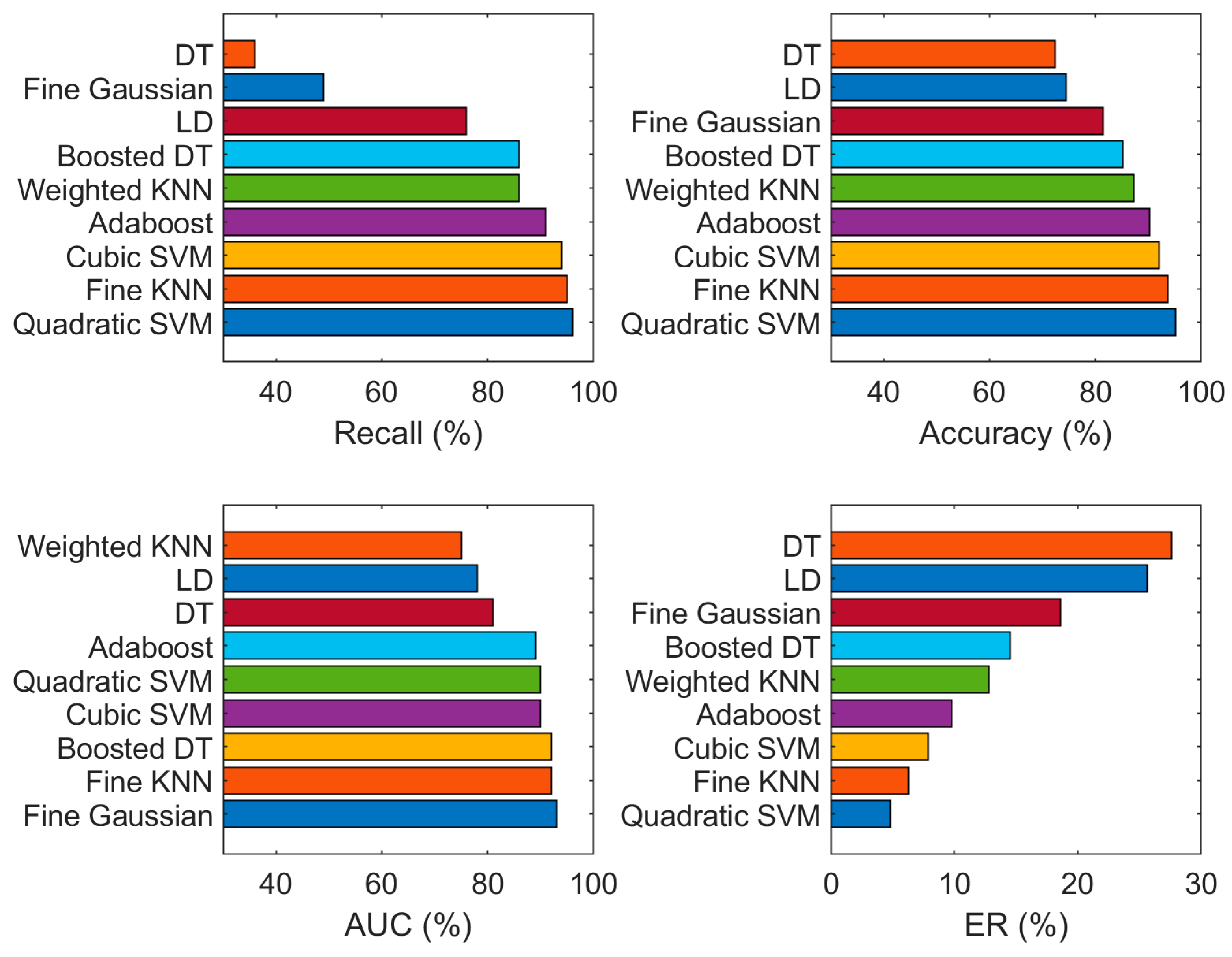
| Classifier | Recall (%) | Accuracy (%) | AUC (%) | ER (%) |
|---|---|---|---|---|
| Cubic Support Vector Machine (SVM) | 94.0 | 92.1 | 90.0 | 7.9 |
| Decision Tree | 36.0 | 72.4 | 81.0 | 27.6 |
| Weighted k-Nearest Neighbor (KNN) | 86.0 | 87.2 | 75.0 | 12.8 |
| Fine Gaussian | 49.0 | 81.4 | 93.1 | 18.6 |
| Fine KNN | 95.0 | 93.7 | 92.0 | 6.3 |
| Boosted Decision Tree | 85.9 | 85.2 | 92.0 | 14.5 |
| Adaboost | 91.0 | 90.2 | 89.0 | 9.8 |
| Linear Discriminate | 76.0 | 74.4 | 78.0 | 25.6 |
| Quadratic SVM | 96.0 | 95.2 | 90.0 | 4.8 |
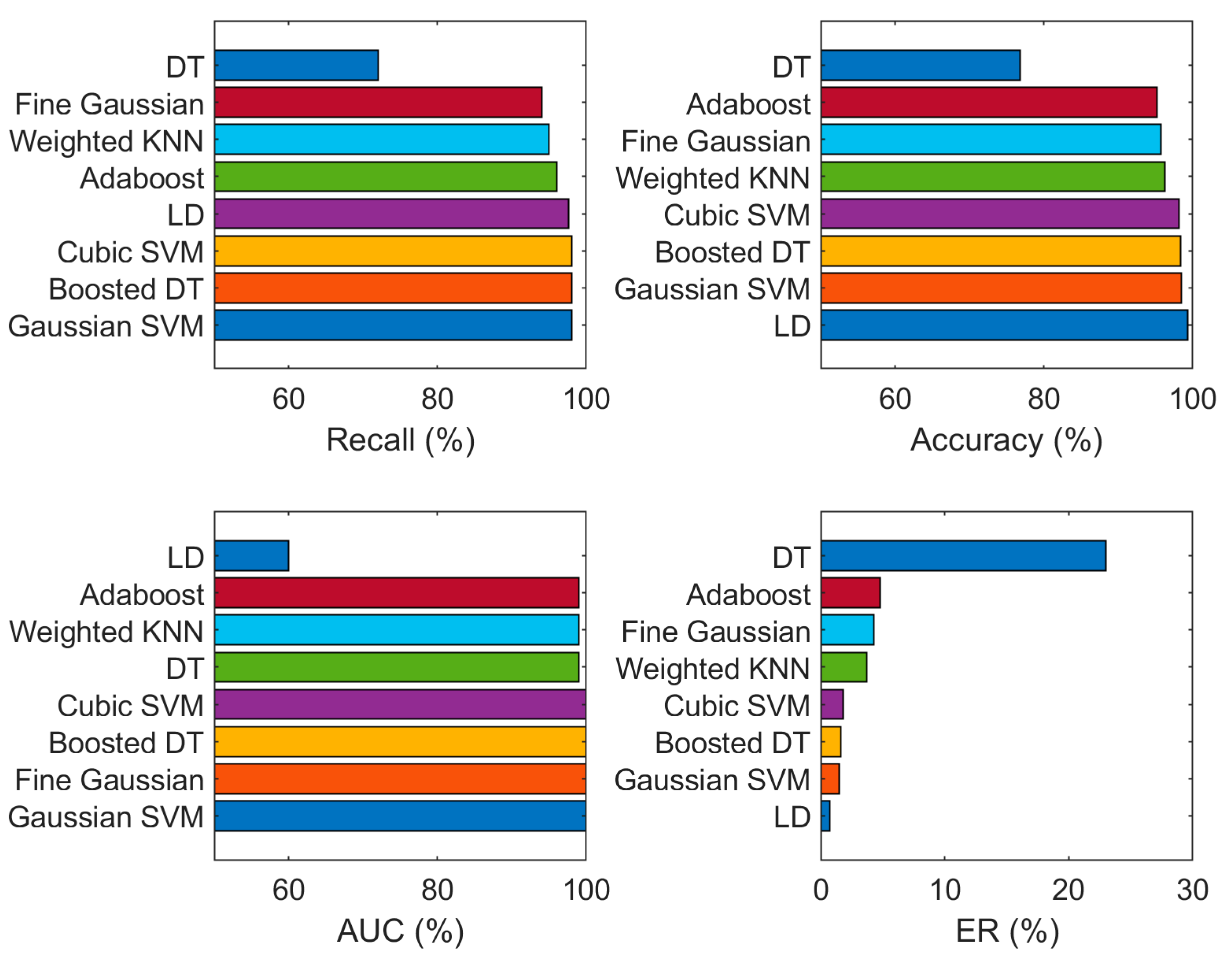
| Classifier | Recall (%) | Accuracy (%) | AUC (%) | ER (%) |
|---|---|---|---|---|
| Gaussian SVM | 98.0 | 98.5 | 100.0 | 1.5 |
| Decision Tree | 72.0 | 76.8 | 99.0 | 23.2 |
| Weighted KNN | 95.0 | 96.3 | 99.0 | 3.7 |
| Fine Gaussian | 94.0 | 95.7 | 100.0 | 4.3 |
| Boosted Decision Tree | 98.0 | 98.4 | 100.0 | 1.6 |
| Adaboost | 96.0 | 95.2 | 99.0 | 4.8 |
| Linear Discriminate | 97.6 | 99.3 | 60.0 | 0.7 |
| Cubic SVM | 98.0 | 98.2 | 100.0 | 1.8 |
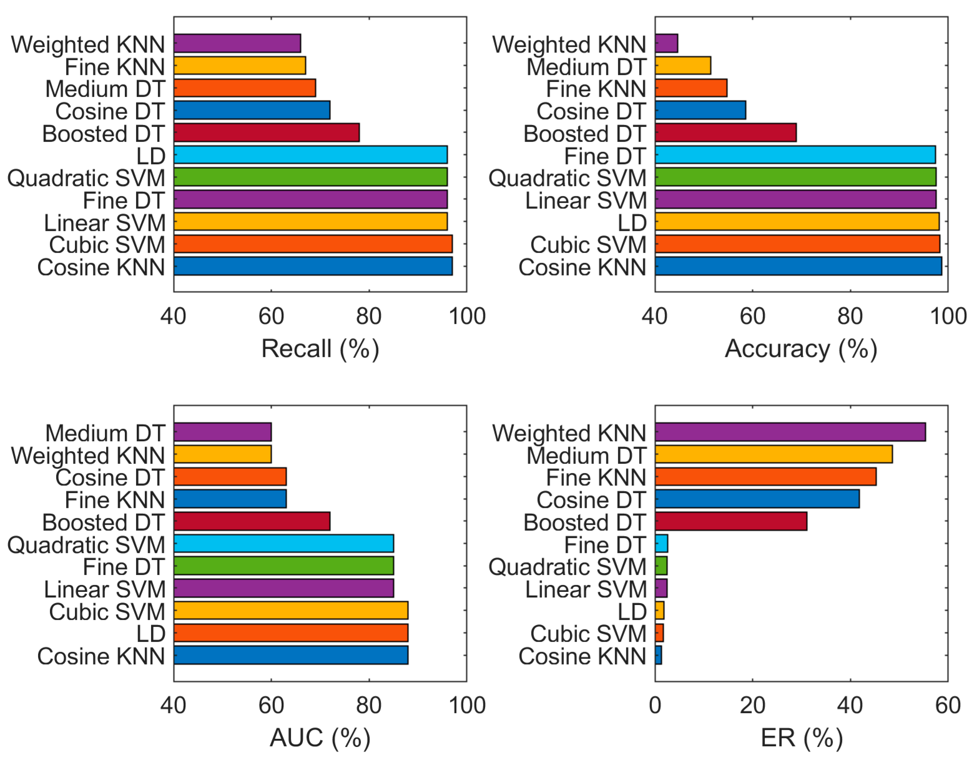
| Classifier | Recall (%) | Accuracy (%) | AUC (%) | ER (%) |
|---|---|---|---|---|
| Linear SVM | 96.0 | 97.5 | 85.0 | 2.5 |
| Fine Decision Tree | 96.0 | 97.4 | 85.0 | 2.6 |
| Weighted KNN | 66.0 | 44.6 | 60.0 | 55.4 |
| Fine KNN | 67.0 | 54.8 | 63.0 | 45.2 |
| Cosine KNN | 97.0 | 98.7 | 88.0 | 1.3 |
| Boosted Decision Tree | 78.0 | 68.9 | 72.0 | 31.1 |
| Quadratic SVM | 96.0 | 97.5 | 85.0 | 2.5 |
| Linear Discriminate | 96.0 | 98.1 | 88.0 | 1.9 |
| Cosine Decision Tree | 72.0 | 58.6 | 63.0 | 41.8 |
| Medium Decision Tree | 69.0 | 51.4 | 60.0 | 48.6 |
| Cubic SVM | 97.0 | 98.3 | 88.0 | 1.7 |
| Classifier | Recall (%) | Accuracy (%) | AUC (%) | ER (%) |
|---|---|---|---|---|
| Linear SVM | 98.0 | 98.5 | 100.0 | 1.5 |
| Fine Decision Tree | 77.0 | 82.8 | 97.0 | 17.2 |
| Weighted KNN | 95.0 | 96.3 | 99.0 | 4.3 |
| Medium KNN | 93.0 | 94.7 | 99.0 | 6.7 |
| Fine KNN | 97.0 | 97.7 | 98.0 | 3.7 |
| Cosine KNN | 96.0 | 96.9 | 99 | 4.9 |
| Boosted Decision Tree | 97.0 | 72.8 | 99.0 | 27.2 |
| Quadratic SVM | 95.0 | 99.1 | 100.0 | 1.0 |
| Linear Discriminate | 97.0 | 97.6 | 99.0 | 3.6 |
| Cosine Decision Tree | 21.0 | 33.5 | 37.0 | 66.5 |
| Medium Decision Tree | 48.0 | 66.8 | 84.0 | 33.2 |
| Cubic SVM | 99.0 | 99.3 | 100.0 | 1.3 |
| Author | Year | Features | Techniques | Accuracy (%) |
|---|---|---|---|---|
| Nataraj et al. [51] | 2011 | GIST feature | Nearest Neighbor | 97.18 |
| Anderson et al. [52] | 2012 | Gaussian kernel features | SVM | 98.0 |
| Dahl et al. [53] | 2013 | Sparse binary features | Neural networks and logistic regression | 86.0 |
| Zhang et al. [54] | 2014 | Graph-based feature | Semantics-based | 93.0 |
| Pascanu et al. [55] | 2015 | Echo state networks (ESNs) and recurrent neural networks (RNNs) for feature extraction | Logistic regression and multilayer perceptron classifier | 98.3 |
| Garcia [56] | 2016 | Texture features | Random Forest | 95.0 |
| Moshiri et al. [57] | 2017 | Filter-based feature | Machine learning techniques | 99.0 |
| Liu et al. [58] | 2017 | N-gram-based texture feature | Shared nearest neighbor (SNN) clustering algorithm | 98.9 |
| Cakir et al. [59] | 2018 | Deep learning-based feature | Gradient boosting | 96.0 |
| Kalash et al. [60] | 2018 | GIST features | CNN-based architecture | 98.5 |
| Naeem et al. [61] | 2019 | Local and global malware pattern (LGMP) features | SVM, KNN | 98.0 |
| Cui et al. [12] | 2019 | CNN-based features | CNN | 97.6 |
| Naeem et al. [62] | 2019 | Combined local and global malware (CLGM) features | DCNN | 98.18 |
| This paper | 2020 | Fused SFTA and deep network features | DCNN (AlexNet, Inception v3) | 99.3 |
© 2020 by the authors. Licensee MDPI, Basel, Switzerland. This article is an open access article distributed under the terms and conditions of the Creative Commons Attribution (CC BY) license (http://creativecommons.org/licenses/by/4.0/).
Share and Cite
Nisa, M.; Shah, J.H.; Kanwal, S.; Raza, M.; Khan, M.A.; Damaševičius, R.; Blažauskas, T. Hybrid Malware Classification Method Using Segmentation-Based Fractal Texture Analysis and Deep Convolution Neural Network Features. Appl. Sci. 2020, 10, 4966. https://doi.org/10.3390/app10144966
Nisa M, Shah JH, Kanwal S, Raza M, Khan MA, Damaševičius R, Blažauskas T. Hybrid Malware Classification Method Using Segmentation-Based Fractal Texture Analysis and Deep Convolution Neural Network Features. Applied Sciences. 2020; 10(14):4966. https://doi.org/10.3390/app10144966
Chicago/Turabian StyleNisa, Maryam, Jamal Hussain Shah, Shansa Kanwal, Mudassar Raza, Muhammad Attique Khan, Robertas Damaševičius, and Tomas Blažauskas. 2020. "Hybrid Malware Classification Method Using Segmentation-Based Fractal Texture Analysis and Deep Convolution Neural Network Features" Applied Sciences 10, no. 14: 4966. https://doi.org/10.3390/app10144966