Active Approaches to Vibration Absorption through Antiresonance Assignment: A Comparative Study

Abstract

Vibration absorption is a core research topic in structural dynamics and the mechanics of machines, and antiresonance assignment is an effective solution to such a problem in the presence of harmonic excitation forces. Due to recent developments in the theory of feedback control systems, the use of active control approaches to antiresonance assignment has been recently gaining more attention in the literature. Therefore, several methods exploiting state feedback or output feedback have been proposed in recent years. These techniques that just rely on servo-controlled actuators are becoming an interesting alternative to active approaches that emulate the well-known Tuned Mass Damper in an active (or semi-active) framework. This paper reviews and compares the most important approaches, with a greater focus on the methods exploiting the concept of control theory without adding new degrees of freedom in the system. The theoretical results, with the underlying theory, are discussed to highlight the key features of each assignment techniques. Several numerical examples where different techniques are applied and compared, also providing some analysis usually neglected in the literature, enrich the paper and demonstrate the key concepts.

1. Introduction	2
Motivations	2
2. Antiresonances in LTI Systems: Theoretical Background	3
3. Overview on Antiresonance Assignment through the Active or Semi-Active Tuned Mass Dampers	4
3.1. The Tuned Mass Damper: An Introduction	4
3.2. The Active Tuned Mass Damper	4
3.3. The Delayed-Resonator	8
3.4. The Semi-active Tuned Mass Damper	9
4. Active Antiresonance Assignment with no Additional Masses	10
4.1. Motivations	10
4.2. State-Feedback Approaches	13
4.3. Output-Feedback Approaches	16
4.4. Numerical Examples of Active Control	18
4.5. The Fully-Active, Virtual Active Tuned Mass Damper	25
4.6. Comparison of Active Vibration Absorption Techniques	28
5 Some Applications of Antiresonance Assignment through Active Control	29
5.1 Antiresonance Assignment in Helicopters	30
5.2 Antiresonance Assignment in Industrial Devices and Machines	30
5.3 Antiresonance Assignment in Buildings and Civil Structures	30
5.4 Antiresonance Assignment and Energy Harvesting	31
6. Conclusions	31
References	32

1. Introduction

Motivations

Vibrations in mechanical systems, such as mechanisms and structures, arise due to their low stiffness-to-mass ratio and light damping. In the case of the harmonic excitation of disturbance forces, an effective approach to absorb vibration is creating antiresonances in the system frequency response. Indeed, when excited at the antiresonance frequencies, the system experiences no (or very small) steady-state vibration in some particular coordinates. One of the first methods, and probably the most famous one, addressing vibration absorption through antiresonance assignment is the seminal work proposed by Frahm in 1911 through his patent [1], where the so-called Tuned Mass Damper (TMD) has been introduced. Thereafter, several approaches and techniques to antiresonance assignment have been developed in the literature and in practical application too. Basically, these methods can be grouped into passive and active. The former consists in the structural modification of the system matrices M, C, K, either by adding degrees-of-freedom (DOFs) or by just modifying the existing ones, without any external power source. In contrast, the latter (together with semi-active approaches) exploit active devices like actuators and sensors, i.e., requiring an external power source.

Passive approaches are usually more efficient under an energy point of view and also cheaper, since no external power, actuators, sensors and controllers are needed. The number of antiresonances to be assigned must be matched by the rank of the modification [2,3] if constraints on the feasible modifications are neglected. In practice, the number of assignable antiresonances is usually smaller than the rank of the modification due to constraints on the feasible modifications of parameters that are usually assumed to avoid bulky modifications to the physical parameters. In term of performances, the system is guaranteed to remain stable due to the symmetric nature of the physical modification [4]. On the other hand, the form of the modification that can be realized physically (described through symmetric, positive-definite or semi positive-definite matrices with an imposed pattern of non-zero terms) is restrictive. Another important feature to consider is that passive techniques have no capability to adapt to changing conditions, that can be tackled just through robustness, and hence their effectiveness can be severely reduced.

These limitations have been motivating the research on antiresonance assignment through active vibration control, where the role of the spring-mass systems is replaced by forces actively exerted by one or more actuators based on sensor measurements. The features of active approaches to antiresonance assignment are complementary to those of passive approaches. Active control enlarges the achievable performances by suitably choosing the actuator and sensor placements and the control logic: for example, the active control can emulate asymmetric modifications of mass and stiffness matrices. By developing adaptive control logic, active approaches can quickly adapt their response to changing environmental conditions and can be targeted to different excitations with different frequencies, thus being effective in a wide frequency range. However, stability is not always ensured; reduced actuator and sensor bandwidths or delayed response, as well as a bad tuning of the controller gains, may degrade the performances and cause instability. On the other hand, the actuators should be, obviously, properly sized in terms of feasible force, displacement, and speed. Additionally, active approaches are more difficult to implement and require significant control efforts, both in term of forces, power, and energy.

The research on active control for antiresonance assignment has been significantly improving in the last decades, leading to two different types of approach:

• methods emulating the passive TMD, with at least one additional mass connected to the system through active springs and dampers;
• methods that do not use additional masses (and related new DOFs) that usually exploit the paradigms of the theory of control.

While a lot of attention has been paid in the literature to the first class of methods that usually translate the research on passive TMDs in an active frame, the approaches with no additional masses have been less discussed, although several researchers have recently investigated them by providing relevant solutions and applications also exploiting new theories on feedback control. This paper therefore provides a comprehensive analysis and critical review of these approaches by providing a detailed discussion and comparison. The underlying mathematical formulations of these methods are briefly presented too, fostering deeper comprehension and collecting the most important equations that could support the users and interested researchers in developing new theoretical contributions in this area. Finally, several numerical examples are provided for highlighting their benefits and drawbacks, as well as to discuss some relevant computational and applicative issues that are often neglected in the literature.

2. Antiresonances in LTI Systems: Theoretical Background

Let us model a linear time-invariant (LTI) vibrating system through $N$ degrees of freedom (DOFs) and its mass matrix $M>0\in {ℝ}^{N\times N}$, its stiffness matrix $K\ge 0\in {ℝ}^{N\times N}$ and its damping matrix $C\in {ℝ}^{N\times N}$. The following system of linear equation of motion is formulated:

$$M\ddot{q}\left(t\right)+C\dot{q}\left(t\right)+Kq\left(t\right)=Bf\left(t\right),$$

(1)

The generalized displacements and the generalized forces are collected in vectors $q(t)\in {ℝ}^N$ and $f(t)\in {ℝ}^N$ respectively, while $B\in {ℝ}^{N\times N}$ is the force distribution matrix. Let us assume that harmonic forces with radian frequency $\omega$ are applied ($j=\sqrt{-1}$). The system response in the frequency domain is therefore:

$$\left(-{\omega }^{2}M+j\omega C+K\right)q\left(j\omega \right)=Bf\left(j\omega \right).$$

(2)

The response displacements are obtained through the receptance matrix $H(j\omega )$ as follows:

$$q\left(j\omega \right)=H\left(j\omega \right)Bf\left(j\omega \right)$$

(3)

where:

$$H\left(j\omega \right)={\left(-{\omega }^{2}M+j\omega C+K\right)}^{-1}.$$

(4)

The receptance $h_{pq}(j\omega )$ from the force applied at the q-th DOF,$f_q(j\omega )$, to the displacement of the p-th DOF, $q_p(j\omega )$ is computed as follows [5,6]:

$$h_{pq}\left(j\omega \right)=\frac{q_p\left(j\omega \right)}{f_q\left(j\omega \right)}={\left(-1\right)}^{p+q}\frac{\det \left(-{\omega }^2{M}_{\overline{q}\overline{p}}+j\omega C_{\overline{q}\overline{p}}+K_{\overline{q}\overline{p}}\right)}{\det \left(-{\omega }^{2}M+j\omega C+K\right)}$$

(5)

The frequencies at which the numerator in Equation (5) becomes null are the antiresonances of $h_{pq}(j\omega )$, that are computed as the roots of:

$$\det \left(-{\omega }^2{M}_{\overline{q}\overline{p}}+j\omega C_{\overline{q}\overline{p}}+K_{\overline{q}\overline{p}}\right)=0$$

(6)

where the adjunct (or adjoint) system, defined through matrices $M_{\overline{q}\overline{p}},C_{\overline{q}\overline{p}},\hspace{0.17em}{K}_{\overline{q}\overline{p}}$$\in {ℝ}^{(N-1)\times (N-1)}$, is obtained by removing the q-th row and p-th column from $M,C,\hspace{0.17em}K$.

The steady-state response of the p-th coordinate is zero if the excitation force applied to the q-th coordinate matches an antiresonance frequency of $h_{pq}(j\omega )$. Antiresonance frequencies will be henceforth denoted as ${\omega }_{z,i}$, with $0\le i\le N-1$. An antiresonance corresponds to a pair of complex and conjugate zeros in the complex plane, $z_i,z_i^{\ast }=-{\xi }_{z,i}{\omega }_{z,i}\pm j{\omega }_{z,i}\sqrt{1-{\xi }_{z,i}}$, where ${\omega }_{z,i}$ is the undamped antiresonance frequency and ${\xi }_{z,i}$ its damping ratio.

3. Overview on Antiresonance Assignment through the Active or Semi-Active Tuned Mass Dampers

3.1. The Tuned Mass Damper: An Introduction

The tuned mass damper (TMD), also called dynamic vibration absorber (DVA) in the literature [7,8,9], is the oldest and most widespread device used to create antiresonance for suppressing oscillations [1,10]. A TMD is an external vibrating system, made by some masses, springs and sometimes dampers, that is properly attached to the primary system to absorb its vibrations. Some review papers have been already proposed (e.g., [11,12]), listing thousands of papers. Therefore, this section aims at discussing some of the main results and the related equations provided by the milestone achievements in TMDs that could be useful for future developments in this research area.

The original idea of the TMD, as well as the subsequent early developments, have been conceived as passive devices, where the external structure is composed only of masses with passive dampers and springs. More recently, active TMDs (ATMD) have been proposed by adopting actuators, controlled through feedback, as active dampers and springs. A third “hybrid” approach has been developed too, leading to semi-active TMDs in which the dampers or springs of the TMD are changed during the operation to adapt them.

3.2. The Active Tuned Mass Damper

The basic idea of an ATMD (Figure 1) is to place an actuator between the primary system to control and the auxiliary mass of the TMD and to make it exert a control force u according to predefined control logic. It is, however, common to place the actuator in parallel with the spring (whose stiffness is $k_a$) and the damper ($c_a$) connecting the primary system to the mass of the TMD [13,14]. In the simple case of a single-DOF ATMD attached to a damped single-DOF primary system, the equation of motion can be easily inferred from the formulation of the passive TMD for a damped system:

$$\left[\begin{array}{cc}m& 0\\ 0& m_a\end{array}\right]\left\{\begin{array}{c}\ddot{q}\left(t\right)\\ {\ddot{q}}_a\left(t\right)\end{array}\right\}+\left[\begin{array}{cc}c+c_a& -c_a\\ -c_a& c_a\end{array}\right]\left\{\begin{array}{c}\dot{q}\left(t\right)\\ {\dot{q}}_a\left(t\right)\end{array}\right\}+\left[\begin{array}{cc}k+k_a& -k_a\\ -k_a& k_a\end{array}\right]\left\{\begin{array}{c}q\left(t\right)\\ q_a\left(t\right)\end{array}\right\}=\left\{\begin{array}{c}{F}_0\sin ({\omega }_{f}t)\\ 0\end{array}\right\}+\left\{\begin{array}{c}u(t)\\ -u(t)\end{array}\right\},$$

(7)

where it is assumed that an external harmonic force with amplitude F₀ and frequency ω_f excites the primary system. The force exerted by the actuator tries to replicate the effect of the mass, the stiffness, and the damping of the classical passive TMD on the basis of the sensed displacement (and in case velocity too) of the masses of the primary system and of the absorber by means of a control law $u(t)=u\left(q\left(t\right),q_a\left(t\right),\dot{q}\left(t\right),{\dot{q}}_a\left(t\right),{\ddot{q}}_a\left(t\right)\right)$. In particular, position feedback emulates the passive spring of the TMD, speed feedback emulates the passive linear damper, and acceleration feedback emulates the TMD mass. The crux is the definition of the suitable control law and the tuning of the parameters, to absorb vibration while accomplishing other tasks such as increasing robustness or decreasing the oscillation of the absorber mass. Due to the similarity between passive and active spring, dampers and masses, the criteria developed to tune passive TMDs can be adopted for ATMD, too, and easily tuned through gain selection. This versatility offered via a wise design of the control law is an advantage of ATMDs over classical passive TMDs. Additionally, since the gains of the control law can be varied during operation, ATMDs can be adapted to variable excitation frequencies.

On the other hand, a relevant drawback of ATMDs compared to passive TMDs is that their effectiveness decreases when “high-frequency” antiresonances are to be created in the case of low actuator bandwidths [15] due to the limitations of the controlled actuator itself (related to electrical and mechanical issues). Such an issue that is usually neglected in the literature is analyzed in Section 4.5.1. A similar issue is the use of sensors with reduced bandwidths, or with time delay in the measurements, as well as the presence of noise (that downgrades bandwidths due to the need of filtering). Another obvious limitation is that the actuator should be properly sized to exert the desired control forces and ensure adequate displacements for effectively damping the unwanted vibrations of the primary system. It should be pointed out that the sizing the system to properly account for the feasible displacements of the TMD mass is an issue that affects passive TMDs, too.

As already mentioned, an effective idea to tune an ATMD is through the various approaches proposed for passive TMDs, such as the one proposed by Den Hartog [10] or other ones optimizing different goals ([16]), by treating the actuator as a spring plus a damper. The degrees of freedom in the choice of the variables to be sensed and in the gain tuning, however, permit further enhancement of the performances and have led to various approaches specifically targeted to ATMDs and SATMDs. For example, in [17], a control algorithm based on the classical optimal feedback control theory has been proposed to reduce both the energy consumption of the actuator and the vibrations of the main system. Eigenvalue assignment exploiting pole placement techniques for the control of the steady-state vibration of tall buildings by means of an ATMD has been proposed in [18]. Fuzzy control logics are adopted too, such as in [19]. An iterative adjoint-based optimization method has been exploited in [20] to design the control law for a vibration absorber. The effectiveness of the techniques is assessed for the control of a two-store frame subject to harmonic base excitation.

Most of the approaches have been developed for systems with symmetric matrices. The optimum parameters of ATMD for an asymmetric system have also been discussed in [21].

Numerical Examples of ATMD with Different Tuning Methods

Let us consider, with no lack of generality, a sample spring-mass-damper system with m = 1 kg, c = 10⁻³ Nsm⁻¹ and k = 1 Nm⁻¹. The goal of this section is to assign an antiresonance ${\omega }_f=\sqrt{\frac{k_c}{m_a}}$ at ω_f = 0.950 rads⁻¹, which corresponds to ω_f = 0.950ω₀ being ${\omega }_0=\sqrt{\frac{k}{m}}$ = 1 rads⁻¹, by means of an ATMD which employs just a physical mass, while the stiffness and the damper of the TMD are fully active, i.e., are exerted by the actuator control force u(t):

$$u\left(t\right)=-k_c\left(q\left(t\right)-q_a\left(t\right)\right)-c_c\left(\dot{q}\left(t\right)-{\dot{q}}_a\left(t\right)\right).$$

(8)

The system is sketched in Figure 2 and its equation of motion are:

$$\left[\begin{array}{cc}m& 0\\ 0& m_a\end{array}\right]\left\{\begin{array}{c}\ddot{q}\left(t\right)\\ {\ddot{q}}_a\left(t\right)\end{array}\right\}+\left[\begin{array}{cc}c& 0\\ 0& 0\end{array}\right]\left\{\begin{array}{c}\dot{q}\left(t\right)\\ {\dot{q}}_a\left(t\right)\end{array}\right\}+\left[\begin{array}{cc}k& 0\\ 0& 0\end{array}\right]\left\{\begin{array}{c}q\left(t\right)\\ q_a\left(t\right)\end{array}\right\}=\left\{\begin{array}{c}{F}_0\sin ({\omega }_{f}t)\\ 0\end{array}\right\}+\left\{\begin{array}{c}u(t)\\ -u(t)\end{array}\right\}.$$

(9)

The control gains in Equation (8) are computed in this example exploiting different approaches, proposed for passive TMDs, to fulfill different control specifications. The selected tuning methods are briefly reported here in

Table 1. Tuning methods for SDOF-TMDs.

Tuning Method Number	1	2	3	4	5
Reference	[10,23]	[24]	[25,26]	[27]	[24]
Tuning rule	$\begin{array}{c}\frac{{\omega }_f}{{\omega }_0}=\frac{1}{1+\mu }\\ {\xi }_d=\sqrt{\frac{3\mu }{8\left(1+\mu \right)}}\end{array}$	$\begin{array}{c}\frac{{\omega }_f}{{\omega }_0}=\frac{1}{1+\mu }\sqrt{\frac{2+\mu }{2}}\\ {\xi }_d=\sqrt{\frac{\mu \left(4+3\mu \right)}{8\left(1+\mu \right)\left(2+\mu \right)}}\end{array}$	$\begin{array}{c}\frac{{\omega }_f}{{\omega }_0}=\frac{1}{1+\mu }\\ {\xi }_d=\sqrt{\frac{\mu }{1+\mu }}\end{array}$	$\begin{array}{c}\frac{{\omega }_f}{{\omega }_0}=\frac{1}{1+\mu }\\ {\xi }_d=\sqrt{\frac{\mu }{2\left(1+\mu \right)}}\end{array}$	$\begin{array}{c}\frac{{\omega }_f}{{\omega }_0}=\frac{1}{\sqrt{1+\mu }}\\ {\xi }_d=\frac{\sqrt{\mu }}{2}\end{array}$

. Each method has been denoted by a number that spans from 1 to 5. The optimization goal fulfilled through each tuning method is here reported (for a more deep analysis see [16,22]):

Tuning 1.

Minimize the maximum displacement of the primary mass.

Tuning 2.

Minimize the total displacement of the primary mass over all frequencies.

Tuning 3.

Minimize the duration of the system transient vibration (the settling time), i.e., maximize the absolute value of the pole real part.

Tuning 4.

Minimize the primary mass displacement and the relative displacement.

Tuning 5.

Minimize the total kinetic energy of the primary mass over all frequencies.

The mass ratio and the damping ratio are denoted by $\mu =\frac{m_a}{m}$ and ${\xi }_d$ respectively.

The response of the primary mass without the absorber and with the ATMDs tuned by different techniques is shown in Figure 3, where the receptance amplitudes are normalized through k, i.e., $\left|kx/F_0\right|$ is shown, so that the proposed result does not depend on m and k of the primary system.

The results of the simulation of the system forced by a harmonic excitation with amplitude F₀ = 10⁻⁴ N at frequency ω_f and controlled by means of the proposed ATMDs leads to the RMS values reported in

Table 2. Summary of the harmonic response of the primary system controlled through different ATMDs and robustness of the closed-loop system.

Tuning Method Number	No Absorber	1	2	3	4	5
qRMS [mm]	0.72	0.39	0.28	0.60	0.45	0.24
qa,RMS [mm]	-	1.49	1.13	1.49	1.49	0.76
u RMS [%]	-	100.08	102.65	100	100.08	104.45
Disk-based gain margin [dB]	-	±0.79	±0.72	±1.16	±0.89	±2.49
Disk-based phase margin [°]	-	±5.2	±4.7	±7.6	±5.9	±5.2

. The RMS value of the control force is reported in percentage with respect to the minimum RMS control force exerted and reveals that the control effort is slightly increased for the 5th tuning method, which is the one that reduces the most the steady-state vibration of both system masses. Besides evaluating these parameters, stability and robustness margins should be analysed in the case of active controlled systems; values of these parameters that are too low might make infeasible the experimental application of ATMDs in some cases (e.g., low-bandwidth actuators, noisy sensors).

The multi-loop robustness margins for the closed-loop system for different ATMDs are summarized in Table 2. It should be noted that tuning 5 [24] leads to the smallest oscillation of the primary system (q_RMS) with the smallest oscillation of the TMD mass (q_a,RMS) while ensuring the highest stability margin of the controlled system (the disk-based gain, the values of which should be as high as possible since they quantify the stability of a closed-loop system against gain or phase variations), hence being more robust. On the other hand, it requires the greatest control effort among the compared techniques, although the increase is smaller than the 5% compared to the less demanding one.

3.3. The Delayed-Resonator

Another interesting application of active TMD is the delayed resonator (DR), also called the time-delayed vibration absorber, that has been introduced in Reference [28]. This device, sketched in Figure 4 and attached to a primary system, is an ATMD with a displacement feedback control force defined through a control gain k_c and a tunable time delay τ_c, such that its equation of motion is:

$$\left[\begin{array}{cc}m& 0\\ 0& m_a\end{array}\right]\left\{\begin{array}{c}\ddot{q}\left(t\right)\\ {\ddot{q}}_a\left(t\right)\end{array}\right\}+\left[\begin{array}{cc}c+c_a& -c_a\\ -c_a& c_a\end{array}\right]\left\{\begin{array}{c}\dot{q}\left(t\right)\\ {\dot{q}}_a\left(t\right)\end{array}\right\}+\left[\begin{array}{cc}k+k_a& -k_a\\ -k_a& k_a\end{array}\right]\left\{\begin{array}{c}q\left(t\right)\\ q_a\left(t\right)\end{array}\right\}=\left\{\begin{array}{c}{F}_0\sin ({\omega }_{f}t)\\ 0\end{array}\right\}+\left\{\begin{array}{c}-k_c{q}_a\left(t-{\tau }_c\right)\\ +k_c{q}_a\left(t-{\tau }_c\right)\end{array}\right\}$$

(10)

The DR must be designed such that a proper tuning of the time-delay enables the damped absorber composed by m_a, c_a and k_a to operate as an undamped absorber tuned at the prescribed antiresonance frequency, i.e., the DR exhibits a non-dissipative (conservative) behavior. In this scenario, complete vibration absorption is achieved.

The DR is tuned in two stages: first, m_a, c_a and k_a are computed as for passive TMDs to assign a prescribed antiresonance ω_f (see, e.g., the tuning rules proposed in Table 1). Secondly, the control gain and the time-delay are computed as follows:

$$\begin{array}{l}{\tau }_c=\frac{1}{{\omega }_f}{\tan }^{-1}\left(\frac{c_a{\omega }_f}{m_a{\omega }_f^2-k_a}\right)\\ k_c=\pm \sqrt{c_a^2{\omega }_f^2+{\left(k_a-m_a{\omega }_f^2\right)}^2}\end{array}$$

(11)

The characteristic equation of the main linear system coupled with a delayed resonator is transcendental. It follows that infinite poles are obtained through this controller. Further, the complex conjugated imaginary pole pair introduced by the absorber is marginally stable to ensure complete vibration absorption. Hence, the authors in [28] deeply discussed the stability and the robustness issues of the system controlled through the DR. Two main stability conditions are obtained with respect to the additive perturbations Δk_c and Δτ_c (of the control gain and of the time delay, respectively). The closed-loop system is stable if:

$$\left\{\begin{array}{c}\Delta k_c<0\\ \Delta {\tau }_c>0\end{array}\right.\hspace{0.17em}\hspace{0.17em}\hspace{0.17em}\hspace{0.17em}\hspace{0.17em}\hspace{0.17em}\hspace{0.17em}\hspace{0.17em}\mathrm{if}\hspace{0.17em}\hspace{0.17em}\hspace{0.17em}\hspace{0.17em}\hspace{0.17em}\hspace{0.17em}\hspace{0.17em}\hspace{0.17em}{\omega }_f<{\omega }_0\sqrt{1-2{\xi }^2}\hspace{1em}\mathrm{and}\hspace{1em}\left\{\begin{array}{c}\Delta k_c<0\\ \Delta {\tau }_c<0\end{array}\right.\hspace{0.17em}\hspace{0.17em}\hspace{0.17em}\hspace{0.17em}\hspace{0.17em}\hspace{0.17em}\hspace{0.17em}\hspace{0.17em}\mathrm{if}\hspace{0.17em}\hspace{0.17em}\hspace{0.17em}\hspace{0.17em}\hspace{0.17em}\hspace{0.17em}\hspace{0.17em}\hspace{0.17em}{\omega }_f>{\omega }_0\sqrt{1-2{\xi }^2}$$

(12)

where ω₀ and ξ are the natural frequency and the damping ratio of the primary system.

The delayed resonator has been adapted to assign two [29] or more antiresonance frequencies [30]. Analytical and experimental results in the design and stability analysis of time-delayed vibration absorbers have been proposed recently in [31,32].

3.4. The Semi-Active Tuned Mass Damper

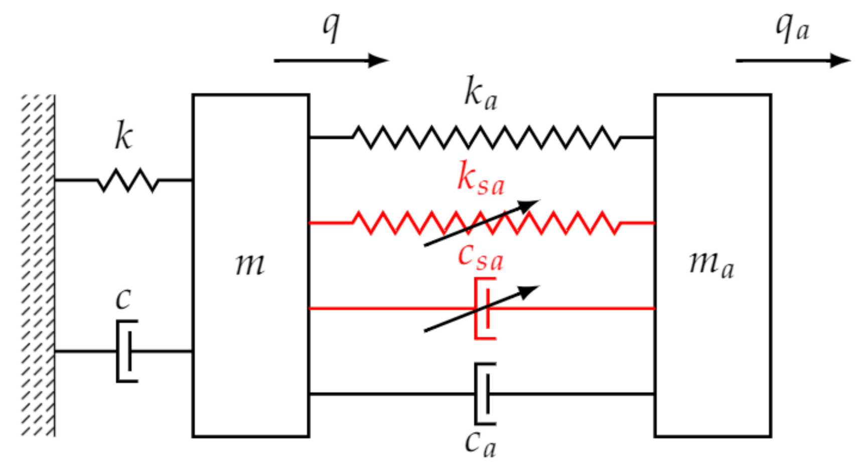
Semi-active TMDs (SATMDs), as represented in Figure 5, have the distinctive feature that a variable stiffness (k_sa) or damper (c_sa) allows adapting the TMD properties to ensure a better tuning than passive TMDs. In the case of the simultaneous use of passive and active variable springs (obtained through the force exerted by an actuator), a small control effort is required whenever the passive part of the TMD is tuned to the frequency to be absorbed, while the active part is adopted to perform adaptation, increasing robustness or accomplishing secondary tasks to optimize performances.

Adjustable dampers are also used in SATMDs by employing variable-orifice hydraulic dampers or dampers based on magnetorheological fluids. Just a small amount of energy is required to modulate the damping of such devices; therefore, lower power requirements with respect to ATMDs are required. This technique is very promising, especially in civil engineering applications, which is the field where SATMDs have found more use due to the lower-frequency contents of the excitations.

In the seminal work [33], the SATMD is compared with the passive TMD and the ATMD, demonstrating the small amount of energy required to adapt damping while ensuring similar performances for the ATMD. Additionally, SATMDs offer reliability, robustness, and cost-effectiveness comparable to passive TMDs.

The design of SATMDs, with time-varying damping, through the optimal control theory has been proposed in [34], and its actual effectiveness to reduce the steady-state response of a SDOF primary structure under harmonic excitation has been assessed. In [35], a magnetorheological damper is used to design a SATMD for a SDOF structure subject to seismic inputs. The magnetorheological SATMD outperforms the classical TMD in the seismic induced vibration suppression.

Single and multiple SATMDs with variable stiffness are proposed in [36] for the control of SDOF and MDOF primary structures. The devices are effective when they have a low damping ratio and the excitation frequency can be tracked.

Semiactive vertical and pendulum TMDs have been proposed in [37], where the authors exploit a variable stiffness pendulum TMD based on the magnetic induction principle to tackle the frequency detuning that occurs due to the changes in the operating environment of the main structures that arise in long-term operations.

A phase control algorithm for the SATMD is proposed in [38]. The idea is inspired by the power flow theory proposed in [39], i.e., the best performances of the TMD are achieved when it remains at a phase lag of −90° to the structure. The algorithm proposed in [38] relies on detecting whenever the phase lag of the TMD is not equal to −90° with respect to the structure and to brings it back through the application of a semi-active variable friction force that slows down the TMD mass block velocity. The effectiveness of the approach is validated through the simplified SDOF model of the Taipei 101 skyscraper.

The performances of SATMD with varying damping for SDOF structures subject to various type of loads have been studied in [40], leading to significantly superior performances of the SATMD with respect to the passive TMD regardless of the type of excitations and providing also cost advantages over the ATMD [41].

SATMDs composed by magneto-sensitive rubber have been studied in [42,43] for the vibration isolation of an infinite-dimensional flexible foundation subject to harmonic excitation varying in a prescribed frequency range.

In [41], inspired by the idea of the fully-active virtual absorber (see Section 4.5) introduced in [44], a SATMD is designed by simultaneously exploiting a linear actuator in parallel with the spring of a passive undamped TMD. The idea is that the actuator sets a virtual TMD with programmable characteristic frequency in such a way that an antiresonance is assigned regardless of the precise knowledge of the dynamics of the primary structure.

In [45], a particular implementation of SATMD is proposed, which is able to change its natural frequency exploiting the idea of generating a force that virtually changes the inertial mass of the device through a dynamic magnetic actuator. The SATMD effectively absorbs each excitation frequency provided by the main rotor of helicopters.

4. Active Antiresonance Assignment with No Additional Masses

4.1. Motivations

Along with the usage of ATMDs and SATMDs, other antiresonance assignment methods have been developed through active control paradigms, usually performed through the feedback of a suitable number of displacements, speed, and acceleration signals. These methods perform vibration absorption without adding new masses, and hence new DOFs, in the system. Although they have been less investigated, the recent theoretical enhancement in the theory of feedback control have boosted a quick growth of their effectiveness in the most recent years, leading to new effective solutions.

Basically, three groups can be defined (see Figure 6) and a summary and comparison of the main methods is provided in Table 3:

• state-feedback control;
• output-feedback control;
• virtual ATMDs.

Table 3. Active antiresonance assignment control techniques: a comparison of existing papers.

Paper Reference	[48,49]	[50]	[51]	[52]	[53]	[54,55,56]	[2]	[57]
Damped system	No	Yes	Yes	Yes	Yes	No	Yes	Yes
Discrete/Continuous system	Discrete	Discrete	Discrete	Discrete	Discrete	Continuous	Discrete	Discrete/Continuous
Symmetric/Asymmetric system	Symm.	Symm.	Both	Symm.	Symm.	Symm.	Symm.	Symm.
1st order formulation/2nd order formulation/Receptance method	2nd order	Recept.	Recept. and 1st order	Recept.	2nd order	2nd order	Recept.	2nd order
State feedback (SF)/Output feedback (OF)	SF.	SF	SF	SF	OF	OF	OF	OF
Collocated controller/Non Collocated	-	-	-	-	Colloc.	Colloc.	Colloc.	Colloc.
Point receptance/Cross receptance	Point	Both	Both	Both	Point	Point	Both	Point
Imposed actuation matrix	No	Yes	Yes	Yes	Yes	Yes	Yes	Yes
Time delay	No	No	No	No	No	No	No	No
Number of assigned zeros	N-1 complex conjugate pairs	Up to N-1 complex conjugate pairs	Up to N-1 complex conjugate pairs	Up to N-1 complex conjugate pairs	1	1 complex conjugate pair	Up to N-1 complex conjugate pairs	1 complex conjugate pair
Control of poles spillover	Yes	Partial	Yes	Partial	No	No	Partial	No

Table 3. Active antiresonance assignment control techniques: a comparison of existing papers.

Paper Reference	[48,49]	[50]	[51]	[52]	[53]	[54,55,56]	[2]	[57]
Damped system	No	Yes	Yes	Yes	Yes	No	Yes	Yes
Discrete/Continuous system	Discrete	Discrete	Discrete	Discrete	Discrete	Continuous	Discrete	Discrete/Continuous
Symmetric/Asymmetric system	Symm.	Symm.	Both	Symm.	Symm.	Symm.	Symm.	Symm.
1st order formulation/2nd order formulation/Receptance method	2nd order	Recept.	Recept. and 1st order	Recept.	2nd order	2nd order	Recept.	2nd order
State feedback (SF)/Output feedback (OF)	SF.	SF	SF	SF	OF	OF	OF	OF
Collocated controller/Non Collocated	-	-	-	-	Colloc.	Colloc.	Colloc.	Colloc.
Point receptance/Cross receptance	Point	Both	Both	Both	Point	Point	Both	Point
Imposed actuation matrix	No	Yes	Yes	Yes	Yes	Yes	Yes	Yes
Time delay	No	No	No	No	No	No	No	No
Number of assigned zeros	N-1 complex conjugate pairs	Up to N-1 complex conjugate pairs	Up to N-1 complex conjugate pairs	Up to N-1 complex conjugate pairs	1	1 complex conjugate pair	Up to N-1 complex conjugate pairs	1 complex conjugate pair
Control of poles spillover	Yes	Partial	Yes	Partial	No	No	Partial	No

Figure 6. A summary of the active antiresonance assignment methods with no additional masses.

Figure 6. A summary of the active antiresonance assignment methods with no additional masses.

Table 3 shows that antiresonance assignment through active control has been usually solved with ad-hoc methods exploiting either the second-order formulation of the system model or receptance, which are two common representations for vibrating systems. At first glance, even the methods developed in the literature for pole placement through state-space, first-order models seem to be suitable for assigning antiresonance by formulating a first-order model of the adjunct system and then by applying standard techniques, such as the place function of MATLAB (which exploits the algorithm proposed in [46]) or the Ackermann’s formula [47]. A deeper investigation reveals that these methods are not suitable for antiresonance assignment for several reasons. First, they require the inversion of the mass matrix of the adjunct system which can be ill-conditioned or even singular (as often happens for cross-receptances). Additionally, the adjunct system is often nearly uncontrollable. A second reason is that standard methods usually need all the poles to be placed it; hence, assigning just a few antiresonances while the other ones are free to assume arbitrary values is not possible. These issues justify the development of methods ad-hoc developed for antiresonance assignment that are discussed in the following paragraphs.

4.2. State-Feedback Approaches

The most eminent researchers in the field of dynamic structural modification also studied the antiresonance assignment through active control and proposed some meaningful results for linear time-invariant systems. The equation of motion of the closed-loop state-feedback controlled system is:

$$\left\{\begin{array}{l}M\ddot{q}\left(t\right)+C\dot{q}\left(t\right)+Kq\left(t\right)=Bf\left(t\right)+B_{C}u\left(t\right)\hfill \\ u\left(t\right)=-{\left[\begin{array}{cc}F& G\end{array}\right]}^T\left\{\begin{array}{c}\dot{q}\left(t\right)\\ q\left(t\right)\end{array}\right\}\hfill \end{array}\right.,$$

(13)

where $u\left(t\right)\in {ℝ}^{N_c}$ is the control force vector (with $N_C$ denoting the number of independent control forces), $B_C\in {ℝ}^{N\times N_c}$ is the control force distribution matrix, and $F,G\in {ℝ}^{N\times N_C}$ are the gain matrices.

Antiresonance assignment has been usually studied in the case of rank-one control, i.e., one independent control force is employed. The control and gain matrices B_C, F and G become vectors, denoted in the following parts of the paper respectively by $b_C$, f and g, leading to the scalar control force:

$$u\left(t\right)=-f^T\dot{q}\left(t\right)-g^{T}q\left(t\right)$$

(14)

As in ATMDs, speed feedback emulates passive dampers, while position feedback emulates passive springs. The use of acceleration feedback is less adopted, mainly because antiresonance frequency can be shifted either through position feedback or through acceleration feedback. Nonetheless, most of the methods proposed in the following can be extended to account for acceleration feedback too.

4.2.1. Assignability of the Zeros through State-Feedback Control

The assignability of the zeros can be computed exploiting the controllability condition for second-order systems that can be found in several books and papers for the assignment of poles (see e.g., [58]), properly formulated for the adjunct system. Indeed, the zeros of the generic receptance h_pq are completely assignable by means of a control force defined by state-feedback algorithm if and only if:

$$\mathrm{rank}\left[\begin{array}{c}{z}_i^2\hspace{0.17em}{M}_{\overline{q}\overline{p}}+z_i\hspace{0.17em}{C}_{\overline{q}\overline{p}}+K_{\overline{q}\overline{p}}\hspace{1em}{B}_C{}_{\overline{q}}\end{array}\right]=N-1$$

(15)

for all the zeros $z_i$ of the open-loop system, where $B_C{}_{\overline{q}}$ is obtained by removing the q-th row from the controller force distribution matrix B_c. On the other hand, the zeros of h_pq are partially assignable whenever the condition in Equation (15) is satisfied just for some zeros.

4.2.2. Antiresonance Assignment for Undamped Systems and Non-Imposed Control Force Distribution Vector

One of the first works addressing active antiresonance assignment in vibrating systems was proposed by Ram in [48,49]. A state feedback method to assign the N-1 zeros of the N-th point receptance together with two complex conjugate poles has been developed, while the remaining poles are imposed to match those of the open-loop system. The method computes the position feedback gain, the control force distribution vectors for the case of sparse force distribution vectors are admitted, and the method has been developed with reference to symmetric, undamped systems, with no possibility of modifying the pole or zero damping. Additionally, the method does not allow for imposing the desired force distribution vector, as it is common in practice and requires distributed actuation even if the rank-one control is performed.

A two-stage procedure is proposed. First, the control gain vector g is computed to assign the two prescribed complex conjugated closed-loop poles $p^c$ to a certain value:

$$g=-\frac{p_1^o-p^c}{p_1^o}K{u}_{r,1}$$

(16)

where $p_1^o$ and $u_{r,1}$ are the eigenvalue-eigenvector pair of the first mode obtained through the open-loop pencil: $Q_o\left(p\right)=K-pM$. In the second stage, the force distribution vector b_c is determined such that the N-1 zeros are assigned. The principal submatrix ${\widehat{Q}}_o\left(z\right)\in {ℝ}^{\left(N-1\right)\times \left(N-1\right)}$, its eigenvalues $z_1^o,\dots ,z_{N-1}^o$ and eigenvectors $u_{z,1},\dots ,u_{z,N-1}$ are obtained and the system matrices are partitioned as follows:

$$b_C=\left\{\begin{array}{c}{\widehat{b}}_C\\ b_{C,N}\end{array}\right\},\hspace{0.17em}\hspace{0.17em}\hspace{0.17em}\hspace{0.17em}\hspace{0.17em}\hspace{0.17em}g=\left\{\begin{array}{c}\widehat{g}\\ g_N\end{array}\right\},\hspace{0.17em}\hspace{0.17em}\hspace{0.17em}\hspace{0.17em}\hspace{0.17em}\hspace{0.17em}K=\left[\begin{array}{cc}\widehat{K}& \widehat{k}\\ {\widehat{k}}^T& k_{NN}\end{array}\right]$$

(17)

Finally, the control force distribution vector that enables us to assign the prescribed closed-loop zeros $z_1^c,\dots ,z_{N-1}^c$ is obtained through:

$${\widehat{b}}_C=-\widehat{K}{U}_{z}r$$

(18)

where $U_z=\left[u_{z,1},\dots ,u_{z,N-1}\right]$ and r is a vector whose coefficients are:

$$r_j=\frac{1}{{\widehat{g}}^T{u}_{z,j}}\frac{z_j^c-z_j^o}{z_j^o}{\displaystyle \prod _{\begin{array}{c}i=1\\ j\ne 1\end{array}}^{N-1}\frac{z_i^c-z_j^o}{z_i^o-z_j^o}}\hspace{0.17em}\hspace{0.17em}\hspace{0.17em}\hspace{0.17em}\hspace{0.17em}\hspace{0.17em}\hspace{0.17em}\mathrm{with}\hspace{0.17em}\hspace{0.17em}j=1,\dots ,N-1$$

(19)

while the N-th entry of $b_C$ is obtained through a prescribed normalization condition.

4.2.3. The Rank-One Receptance Method: The Original Formulation

A milestone in the field of active control of LTI vibrating systems is the work proposed by Mottershead and Ram in [50], where the assignment of poles and zeros is interpreted as a rank-1 modification to the dynamic stiffness matrix of the system, leading to a receptance-based formulation. This method has been firstly developed to perform the pole placement through full-state feedback control of symmetric LTI systems with rank-one control. Then, a mathematical frame has been developed with reference to the adjoint system to assign a set of zeros, as well as to concurrently assign a set of poles.

A meaningful result provided by [50] shows that the computation of the gain vector $k=\left\{\begin{array}{c}f\\ g\end{array}\right\}\in {ℝ}^{2N}$ for the assignment of n_z zeros through full-state feedback can be written as a linear system:

$$\left[\begin{array}{cc}{z}_1{t}_1^T& t_1^T\\ z_2{t}_2^T& t_2^T\\ ⋮& ⋮\\ z_{n_z}{t}_{n_z}^T& t_{n_z}^T\end{array}\right]\left\{\begin{array}{c}f\\ g\end{array}\right\}=\left\{\begin{array}{c}-h_{pq}\left(z_1\right)\\ -h_{pq}\left(z_2\right)\\ ⋮\\ -h_{pq}\left(z_{n_z}\right)\end{array}\right\},$$

(20)

where the i-th vector $t_i\in {ℂ}^N$ is defined as follows:

$$t_i=h_{pq}\left(z_i\right)H\left(z_i\right)b_C-\left[e_p^{T}H\left(z_i\right)b_C\right]H\left(z_i\right)e_q.$$

(21)

The use of receptance-based formulation has the advantage that the method just relies on the measured receptance, and hence it does not require the knowledge of the M, C, and K matrices. Another great advantage of receptance-based formulation, for pole placement too, is the good numerical conditioning. On the other hand, receptances are sometimes difficult to measure for rotational coordinates [2]. Additionally, the practice of the implementation of state feedback control usually replaces the measured state with the estimated one by implementing state observers, which usually require first-order, state-space formulations.

The receptance-based approach formulated in [50] has been subsequently exploited for some particular applications by adapting the formulation to the specific feature of the model under investigation. For example, in [59] it is applied to an active control for pole and zero assignment in viscoelastic systems.

4.2.4. The Rank-One Receptance Method with Regional Pole Placement

The main limitation of solving Equation (20) alone is that it does not account for spillover on the unassigned 2N-n_z poles, and hence it does not ensure the asymptotic stability of the controlled system. To tackle this issue, a two-stage approach has been recently proposed in [51] by the authors of this paper, handling asymmetric and ill-conditioned systems too.

Let us first recast the linear system in Equation (20) in a more compact form:

$$Gk=y$$

(22)

with the obvious meaning of G and y. Since the linear system in Equation (22) is underdetermined, as a matter of fact, $G\in {ℂ}^{n_z\times 2N}$ with $n_z\le 2\left(N-1\right)$, its solution k can be expressed as the sum of the particular solution of the non-homogeneous equation, denoted k₀, and a solution of the homogeneous system GVk_r = 0, hence:

$$k=k_0+V{k}_r$$

(23)

where the columns of matrix V span the null space of G, i.e., $V\in \mathrm{span}\left(\ker \left(G\right)\right)$. A similar approach exploiting the null space of the linear system has been successfully applied to pole assignment, too [60,61].

In the first stage of the method proposed in [51], the particular solution k₀ is computed to assign the prescribed n_z zeros for receptance h_pq. In the second stage, the set of solutions of the homogeneous system related to the zero-assignment problem is exploited to cluster the closed-loop system poles into D-stable regions, i.e., portions of the complex plane that ensure stability and the prescribed dynamic properties for the closed-loop system. In such a way, in the second-stage of the method, the powerful LMI theory [60,61,62,63] is adopted to compute the (2N-n_z)-dimensional vector k_r by solving the semi-definite programming:

$$\begin{array}{l}\min \hspace{0.17em}\hspace{0.17em}\hspace{0.17em}\hspace{0.17em}\hspace{0.17em}\hspace{0.17em}\hspace{0.17em}{‖p‖}_2^2\\ \mathrm{subj}\hspace{0.17em}\hspace{0.17em}\hspace{0.17em}\hspace{0.17em}\hspace{0.17em}\hspace{0.17em}\hspace{0.17em}{\Psi }_D\left(A_1,p,\hspace{0.17em}X\right)\prec 0\\ \hspace{0.17em}\hspace{0.17em}\hspace{0.17em}\hspace{0.17em}\hspace{0.17em}\hspace{0.17em}\hspace{0.17em}\hspace{0.17em}\hspace{0.17em}\hspace{0.17em}\hspace{0.17em}\hspace{0.17em}\hspace{0.17em}\hspace{0.17em}\hspace{0.17em}\hspace{0.17em}X=X^T\succ 0\end{array}$$

(24)

where:

$$\begin{array}{c}A=\left[\begin{array}{cc}-M^{-1}C& -M^{-1}K\\ I& 0\end{array}\right]\hspace{0.17em}\hspace{0.17em}\hspace{0.17em}\hspace{0.17em}\hspace{0.17em}\hspace{0.17em}\hspace{0.17em}B=\left[\begin{array}{c}{M}^{-1}{b}_C\\ 0\end{array}\right]\\ A_1=A-B{k}_0^T\\ p=XV{k}_r\\ {\Psi }_D\left(A_1,p,\hspace{0.17em}X\right)=R\otimes X+Z\otimes \left(A_{1}X-B{p}^T\right)+Z^T\otimes {\left(A_{1}X-B{p}^T\right)}^T\end{array}$$

(25)

By adopting suitable values for matrices R and Z, several LMI regions with different shapes are obtained [63].

4.2.5. The Rank-One Receptance Method with Integral Action

An extension of the receptance method in the case of the rank-one control has been proposed in [52] to include the integral control action by adopting a formulation of the integral similar to the one previously proposed in [64] for pole placement in flexible link mechanisms with state feedback and integral action. The use of an integral term is widely adopted in positioning control to improve disturbance rejection and reduce steady-state errors; in contrast, it is infrequently adopted whenever the sole goal is assigning poles or zeros, since proportional and derivative (PD) controllers, i.e., position and speed feedback, suffice to perform the assignment.

The scalar control force of the resulting PID controller is $u\left(t\right)=-f^T\dot{q}\left(t\right)-g^{T}q\left(t\right)-n^T{\displaystyle {\int }_0^{T_f}q\left(t\right)}\mathrm{d}t$, where n is the vector of the integral gains, and Equation (20) is adapted as follows:

$$\left[\begin{array}{ccc}{z}_1{t}_1^T& t_1^T& \frac{t_1^T}{z_1}\\ z_2{t}_2^T& t_2^T& \frac{t_2^T}{z_2}\\ ⋮& ⋮& ⋮\\ z_{n_z}{t}_{n_z}^T& t_{n_z}^T& \frac{t_{n_z}^T}{z_{n_z}}\end{array}\right]\left\{\begin{array}{c}f\\ g\\ n\end{array}\right\}=\left\{\begin{array}{c}-h_{pq}\left(z_1\right)\\ -h_{pq}\left(z_2\right)\\ ⋮\\ -h_{pq}\left(z_{n_z}\right)\end{array}\right\}$$

(26)

4.3. Output-Feedback Approaches

The need for a state observer to feed back the estimated state in lieu of the actual one is partially overcome using output feedback. On the other hand, the number of assignable zeros decreases, as discussed in the following, and the achievable performances of output feedback are usually less than those of state-feedback.

4.3.1. Assignment for Point-Receptances with Collocated Controllers through Unit-Rank Output Feedback

Antiresonance assignment for point-receptances by means of output feedback has been effectively solved in [53] by Singh and Ram. The authors developed a closed-form solution for damped vibrating systems in the case of a collocated control (i.e., the control actuator and the feedback sensor are in the same position). The position feedback gain k_c and the velocity feedback gain c_c for assigning antiresonance ${\omega }_z^d$ through the scalar control force $u\left(t\right)=-k_c{x}_{N-1}\left(t\right)-c_c{\dot{x}}_{N-1}\left(t\right)$ are computed through the following relation:

$$k_c+j{\omega }_z^d{c}_c=-\frac{\det \left(-{\left({\omega }_z^d\right)}^2\widehat{M}+j{\omega }_z^d\widehat{C}+\widehat{K}\right)}{\det \left(-{\left({\omega }_z^d\right)}^2\tilde{M}+j{\omega }_z\tilde{C}+\tilde{K}\right)},$$

(27)

where $\widehat{M},\hspace{0.17em}\widehat{C},\hspace{0.17em}\widehat{K}$ are obtained by removing the N-th row and column from M, C, and K (i.e., the point receptance index). $\tilde{M},\hspace{0.17em}\tilde{C},\hspace{0.17em}\tilde{K}$ are, in turn, computed from $\widehat{M},\hspace{0.17em}\widehat{C},\hspace{0.17em}\widehat{K}$, removing the row and columns corresponding to the (N-1)-th row and column of M, C, K (i.e., the index of the collocated actuator-sensor pair). The method is validated by means of numerical example on systems with few coordinates.

Few other approaches have been proposed in the literature to solve some specific problems. In [54,55,56], the problem of absorbing the harmonic response at the end of an axially vibrating rod is considered. The authors proposed different strategies, e.g., formulations based on the deformation or on the spectral data are carried out to compute the collocated displacement feedback control gain at a particular location that ensures the assignment of a prescribed antiresonance frequency.

4.3.2. Assignment for Point-Receptances with Collocated Controllers through Multi-Rank Output Feedback

The receptance-based approach has been further exploited by Mottershead and his co-workers in [2] to assign zeros to a point-receptance through more collocated pairs of sensors and actuators. The closed-loop system is represented as follows, where C_o is the output sensing matrix and $F_y,G_y$ are the gain matrices:

$$\left\{\begin{array}{l}M\ddot{q}\left(t\right)+C\dot{q}\left(t\right)+Kq\left(t\right)=Bf\left(t\right)+B_{C}u\left(t\right)\hfill \\ u\left(t\right)=-{\left[\begin{array}{cc}{F}_y& G_y\end{array}\right]}^T\left\{\begin{array}{c}\dot{y}\left(t\right)\\ y\left(t\right)\end{array}\right\}\hfill \\ \left\{\begin{array}{c}\dot{y}\left(t\right)\\ y\left(t\right)\end{array}\right\}=\left[\begin{array}{cc}{C}_O& 0\\ 0& C_O\end{array}\right]\left\{\begin{array}{c}\dot{q}\left(t\right)\\ q\left(t\right)\end{array}\right\}\hfill \end{array}\right.,$$

(28)

Collocated pairs are adopted, leading to $C_O=B_C^T$, since stability is ensured if actuators and sensors do not introduce phase-lag [65]. The assignment of n_z zeros for p-th point receptance is formulated as the solution of the following condition:

$${\left[\mathrm{adj}\left(I+H\left(z_i\right)B_C\left(G_y^T+z_i{F}_y^T\right)C_O\right)H\left(z_i\right)\right]}_{pp}=0\hspace{0.17em}\hspace{0.17em}\hspace{0.17em}\hspace{0.17em}\hspace{0.17em}\mathrm{with}\hspace{0.17em}\hspace{0.17em}i=1,\dots ,n_z$$

(29)

where the pp-th receptance of the adjunct matrix is set to zero for all the prescribed antiresonances z_i. Poles are assigned together with the zeros, and the gain matrices are imposed to be symmetric and positively semi-definite. Equation (29) leads to characteristic equations that are nonlinear in the control gains; hence, there may be one or more real solutions, or there may be no solution. On the other hand, the assumption of diagonal and positive semi-definite gain matrices simplifies the numerical solutions while ensuring that the control does not cause instability. The authors themselves recognize that using fully populated symmetric gain matrices would enlarge the achievable results by allowing more poles and zeros to be assigned than the number of actuators and sensors, or to accomplish secondary tasks, such as reducing the control effort or increasing robustness. To increase robustness of the closed-loop system in a prescribed frequency range from ${\omega }_{\min }$ to ${\omega }_{\max }$, the authors introduced a constraint in the solution of Equation (29) through the minimum singular ($\underset{\_}{\sigma }$) value of the matrix in Equation (30):

$$\begin{array}{c}\underset{\_}{\sigma }\left(I+H\left(j\omega \right)B_C\left(G_y^T+j\omega F_y^T\right)C_O\right)>r\\ {\omega }_{\min }\le \omega \le {\omega }_{\max }\end{array},$$

(30)

r is the minimum allowable value over the selected frequency range.

The paper also provides the experimental application of the method to a T-shaped plate.

4.3.3. Assignment for Point-Receptances through Unit-Rank Output Feedback with Time Delay

Active antiresonance assignment for symmetric LTI systems with time delay has been investigated by Singh et al. in [57], where output feedback is exploited. The authors refer to their method as “nodal control”, in contrast to the full-state feedback control. Due to the presence of time delay τ in sensor measurements, the characteristic equation of the closed-loop system is transcendental. Therefore, it has an infinite number of roots: 2N roots are the so-called “primary roots”, while an infinite number of “secondary roots” (or “latent roots”) is due to the presence of the time delay and appears in the controlled system [60,66,67]. The authors, in [57], exploited a low-order Taylor series approximation of the time-delay and computed the control gains for the assignment of antiresonance to the point-receptance of a non-conservative system through a single-input and single-output control. The scalar control force is therefore:

$$u\left(t-\tau \right)=-k_c{x}_{N-1}\left(t-\tau \right)-c_c{\dot{x}}_{N-1}\left(t-\tau \right)$$

(31)

By exploiting the second-order model and some mathematical developments similar to those employed in [53], a closed-form solution of the position feedback gain k_c and the velocity feedback gain c_c is obtained:

$$k_c=\frac{{\omega }_z^d\tau \mathrm{Im}\left(\varphi \right)-\mathrm{Re}\left(\varphi \right)}{{\tau }^2{\left({\omega }_z^d\right)}^2+1},\hspace{0.17em}\hspace{0.17em}\hspace{0.17em}\hspace{0.17em}\hspace{0.17em}\hspace{0.17em}\hspace{0.17em}{c}_c=\frac{\mathrm{Im}\left(\varphi \right)+{\omega }_z^d\tau \mathrm{Re}\left(\varphi \right)}{{\omega }_z^d\left({\tau }^2{\left({\omega }_z^d\right)}^2+1\right)}$$

(32)

where

$$\varphi =-\frac{\det \left(-{\left({\omega }_z^d\right)}^2\widehat{M}+j{\omega }_z^d\widehat{C}+\widehat{K}\right)}{\det \left(-{\left({\omega }_z^d\right)}^2\tilde{M}+j{\omega }_z\tilde{C}+\tilde{K}\right)}$$

(33)

The proposed approximation of the time-delay holds only if the time delay is very small. The limitation of this method is that the stability of the controlled system is not guaranteed, as the authors themselves state in [57]. Additionally, the method is developed to assign undamped antiresonance. A second formulation based on the full Taylor series (i.e., the series with infinite terms) is proposed, too. Again, stability is not always ensured for some delays due to the secondary roots that are not imposed in the control synthesis.

4.4. Numerical Examples of Active Control

4.4.1. Numerical Examples of Active Control: Assignment of a Single Antiresonance through State or Output Feedback

The goal of this section is to assign an antiresonance frequency through the techniques proposed in [53] for output feedback collocated control (Equation (27)), and [50] for state feedback (Equation (20)), and then to compare the results. Let us consider the system sketched in Figure 7 that has been taken from the literature as a test case [68,69,70,71,72]. The system is made of six lumped masses and springs of unitary value (1 kg for the masses and 1 Nm⁻¹ for the springs). The system is lightly damped and the Rayleigh damping model is assumed (see e.g., [73]): the mass and stiffness proportional coefficients are, respectively, a = 1 10⁻² s⁻¹, b = 1 10⁻⁶ s, such that C = aM+bK [74,75].

Let us consider the point-receptance h_3,3(jω), where an undamped antiresonance is assigned at 1.000 rads⁻¹ (i.e., the zero locations are 0 ± 1j) exploiting one control force whose force distribution vector is $b_C^{}$ = [1, 0, 0, 0, 0, 0]^T. Such a choice ensures the partial controllability of the adjoint system since only two zeros ensure a rank of the controllability matrix equal to 5. In the case of output-feedback, the output measurement matrix for the collocated control is therefore $C_O=b_C^T$.

The zeros obtained by means of the proposed controllers are reported in

Table 4. Zeros of the original and modified receptance h_3,3(jω) with the different controllers to assign a complex conjugate zero pair.

Original System Zeros	Output-Feedback Method [53]	State-Feedback Method [50] Solved Through Pinv	State-Feedback Method [50] Solved Through Mldivide
−0.005 ± 0.720 j	−0.005 ± 0.720 j	−0.005 ± 0.720 j	−0.005 ± 0.720 j
−0.005 ± 1.176 j	0 ± 1.000 j	0 ± 1.000 j	0 ± 1.000 j
−0.005 ± 1.520 j	−0.005 ± 1.520 j	−0.005 ± 1.520 j	−0.005 ± 1.520 j
−0.005 ± 1.902 j	−0.004 ± 1.871 j	−0.005 ± 1.897 j	−0.004 ± 1.871 j
−0.005 ± 2.042 j	−0.005 ± 2.042 j	−0.005 ± 2.042 j	−0.005 ± 2.042 j

, while the control gains are reported in

Table 5. The control gains in the numerical example of zeros assignment through unit-rank active control.

Gain Vector k	Output-Feedback Method [53]	State-Feedback Method [50] Solved Through Pinv	State-Feedback Method [50] Solved Through Mldivide
Velocity gains f
f1	−0.0125	−0.0100	−0.0125
f2	-	−0.0060	0
f3	-	0	0
f4	-	0	0
f5	-	0	0
f6		0	0
Position gains g
g1	−0.500	−0.4000	−0.500
g2	-	−0.2000	0
g3	-	0	0
g4	-	0	0
g5	-	0	0
g6	-	0	0
${‖k_0‖}_2^{}$	0.5002	0.4774	0.5002

. The unit-rank receptance-based method [50] leads to an underdetermined linear system whenever antiresonance is assigned. Two solutions are here compared: the first solution is obtained when solving Equation (26) by means of the pseudo-inverse of the coefficient matrix (that is referred to in the tables as pinv), that leads to the minimum norm solution; the second one solve the underdetermined system by exploiting the mldivide function of MATLAB, which aims to obtain the fewest possible nonzero components in the control gain vector by exploiting a QR-decomposition algorithm [76] which does not lead necessarily the minimum norm solution. In control system design, minimum norm solution is attractive since it offers a heuristic rule to reduce the actuator effort and noise influence; conversely, the solution with the fewest possible nonzero components enables us to design controllers with fewer coordinates to be measured (i.e., output-feedback controllers).

In the case of solving Equation (20) for the assignment of a complex conjugated pair of zeros through pinv the gains vector k₀ is fully populated while exploiting mldivide only two entries of k₀ are not-null, thus matching in this example the solution of the output-feedback solution.

It follows that, for assigning a pair of complex conjugated zeros (i.e., an antiresonance), the output-feedback controller, as well as the state-feedback controller obtained through mldivide, both lead to a proportional-derivative controller.

The open-loop and closed-loop receptances h_3,3(jω) are compared in Figure 8 to confirm the fulfilment of the assignment task.

The same control task is performed through the state feedback with integral action by solving the system in Equation (26) [52] and comparing the results provided pinv and mldivide. The open-loop and closed-loop zeros of receptance h_3,3(jω) are reported in

Table 6. Zeros of the original and modified receptance h_3,3(jω) with the controller with integral action to assign a complex conjugate zero pair.

Original System Zeros	Method [52] Solved Through Pinv	Method [52] Solved Through Mldivide
-	−0.0049	-
−0.005 ± 0.720 j	−0.005 ± 0.720 j	−0.005 ± 0.720 j
−0.005 ± 1.176 j	0 ± 1.000 j	0 ± 1.000 j
−0.005 ± 1.520 j	−0.005 ± 1.520 j	−0.005 ± 1.520 j
−0.005 ± 1.902 j	−0.005 ± 1.897 j	−0.004 ± 1.871 j
−0.005 ± 2.042 j	−0.005 ± 2.042 j	−0.005 ± 2.042 j

; the 2-norm of the control gains are listed in

Table 7. Control gain 2-norms in the numerical example of the assignment of zeros through unit-rank active control with integral action.

Gain Vector k	Method [52] Solved Through Pinv	Method [52] Solved Through Mldivide
${‖f‖}_2^{}$	0.0059	0.0125
${‖g‖}_2^{}$	0.4472	0.5000
${‖n‖}_2^{}$	0.0059	0
${‖k_0‖}_2^{}$	0.4473	0.5002

. The minimum-norm computation (i.e., pinv) leads to a proportional-integral-derivative controller. In contrast, computing the controller through mldivide leads to the proportional-derivative controller obtained in Table 5: indeed, such a controller configuration is enough to assign the desired antiresonance.

4.4.2. Numerical Examples of Active Control: Assignment of More Antiresonances

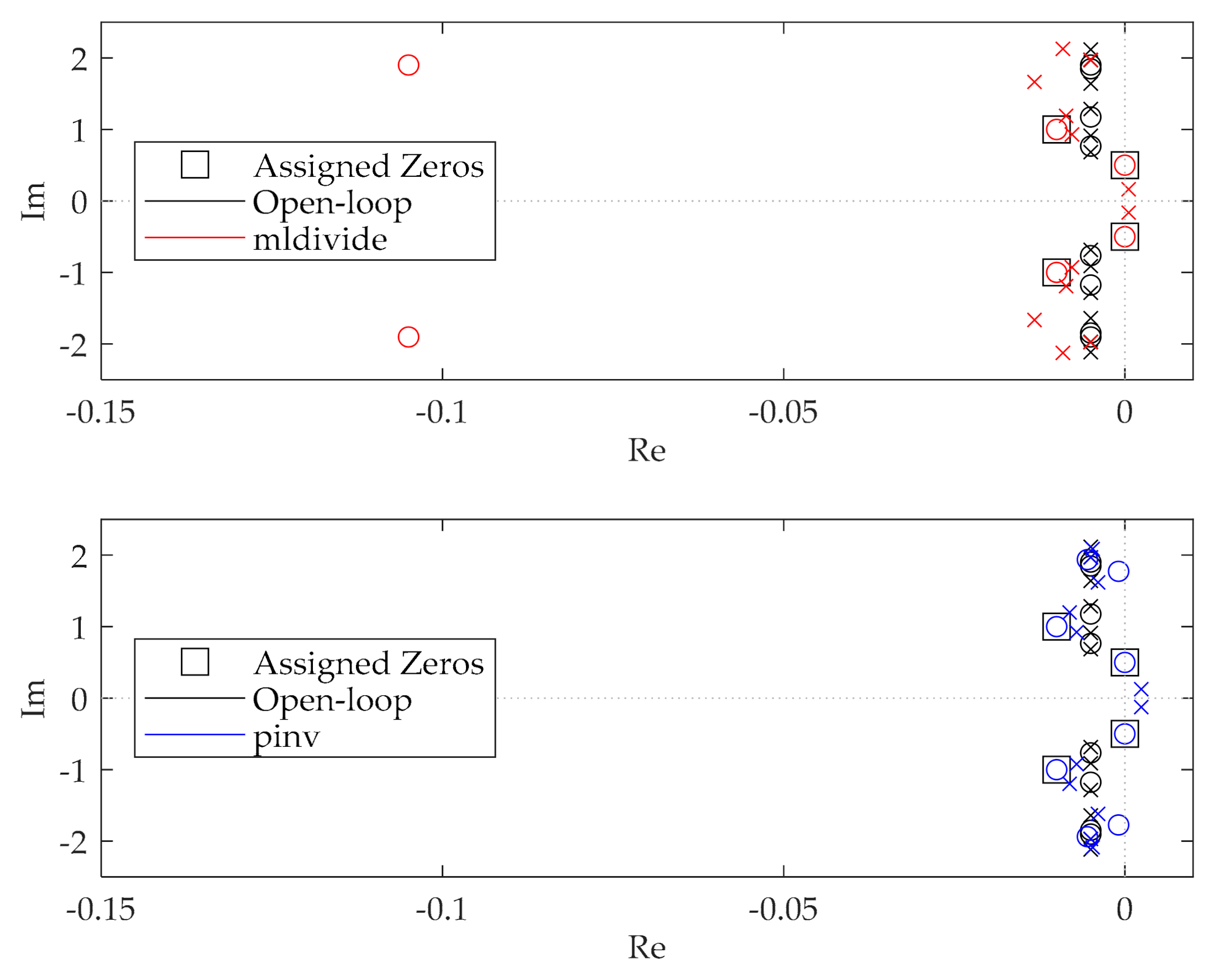
The goal of this section is to assign two antiresonances, i.e., two complex conjugate pairs of zeros (0 ± 0.5j and −0.01 ± 1j), in the cross-receptance h_3,4(jω). For example, let us consider $b_C^{}$ = [1, 0, 0, 0, 1, 0]^T, which ensures the complete assignability of the receptance zeros. The obtained zeros are reported in

Table 8. Zeros of the original and modified receptance h_3,4(jω) with the different controllers to assign two complex conjugate zero pairs.

Original System Zeros	State-Feedback Method [50] Solved Through Pinv	State-Feedback Method [50] Solved Through Mldivide
−0.005 ± 0.765 j	0 ± 0.500 j	0 ± 0.500 j
−0.005 ± 1.176 j	−0.010 ± 1.000 j	−0.010 ± 1.000 j
−0.005 ± 1.848 j	−0.001 ± 1.774 j	−0.105 ± 1.902 j
−0.005 ± 1.902 j	−0.006 ± 1.938 j	0.082 ± 1.910 j

, by solving again Equation (26) with the two methods discussed in Section 4.4.1; the control gains are shown in

Table 9. Control gains in the numerical example of the assignment of zeros through the unit-rank active control for receptance h_3,4(jω).

Gain Vector k0	State-Feedback Method [50] Solved Through Pinv	State-Feedback Method [50] Solved Through Mldivide
Velocity gains f
f1	0.0129	0.0263
f2	0.0093	0
f3	0	0
f4	−0.0093	0
f5	−0.0201	0
f6	−0.0324	−0.0580
Position gains g
g1	−0.391	−0.500
g2	−0.109	0
g3	0	0
g4	0.109	0
g5	−0.457	0
g6	−0.609	−0.920
${‖k_0‖}_2^{}$	0.8707	1.0495

.

Once again, the assignment task is correctly fulfilled. As expected, the solution provided by the pseudoinverse leads to a smaller 2-norm of vector k₀, with the drawback of obtaining a fully populated gain vector which requires more sensors or a state observer. However, it leads to a pair of RHCP complex conjugate poles as well as the solution provided by mldivide, as shown through the pole-zero map in Figure 9. This fact highlights that the solution of the linear system in Equation (20) should be done carefully to ensure stability. This issue is tackled in Section 4.4.3 through the method proposed in [51] to cluster the closed-loop poles to ensure the stability of the closed-loop system.

If the integral action is included too, as in [52], both the solutions of Equation (26) obtained through mldivide and pinv lead to RHCP poles, as shown in Figure 10.

4.4.3. Numerical Examples of Active Control: Assignment of More Antiresonances with Embedded an a-Priori Stability Condition

The test case of Section 4.4.2 is solved in this section through the two-stage approach proposed in [51] to ensure that the closed-loop poles must belong to the left half of the complex plane for asymptotic stability, i.e., introducing a LMI with R = 0 and Z = 1 in Equation (25).

The first stage is solved, again, through the pinv and mldivide functions leading to the same control gains k₀ reported in Table 9 and whose pole-zero map are shown in Figure 10. In the second stage, the semi-definite programming in Equation (24) is solved through the YALMIP toolbox for MATLAB [77] adopting Mosek as the solver. Figure 11 highlights that in both cases, the control gains k = k₀ + Vk_r (reported in

Table 10. Stabilizing control gains obtained in the second stage of the method in the numerical example of the assignment of zeros through the unit-rank active control for receptance h_3,4(jω) with LMI constraints.

Gain Vectork = k0+Vkr	State-Feedback Method [51](k0 Obtained Through Pinv)	State-Feedback Method [51](k0 Obtained Through Mldivide)
Velocity gains f
f1	0.0134	0.0274
f2	0.0227	0.0119
f3	0.0141	0.0131
f4	0.0052	0.014
f5	−0.0309	−0.0192
f6	−0.0244	−0.0439
Position gains g
g1	−0.391	−0.500
g2	−0.109	0
g3	0	0
g4	0.109	0.001
g5	−0.458	0
g6	−0.608	−0.921
${‖k‖}_2^{}$	0.8711	1.0495

) ensure the asymptotic stability of the closed-loop system, since the closed-loop poles belong to the LHCP (whose shape is highlighted by the dashed line in Figure 11).

The steady-state responses of the open-loop and closed-loop systems, controlled with the stabilizing gains computed through mldivide, are compared in Figure 12a to corroborate the capability of absorbing vibrations when a harmonic disturbance with a frequency equal to 0.500 rads⁻¹ excites coordinate 4. The control force is reported in Figure 12b.

4.5. The Fully-Active, Virtual Active Tuned Mass Damper

The TMDs discussed so far in Section 3 introduce at least one additional DOF in the system due to the mass of the TMD. A different approach in the design of ATMDs is the so-called virtual ATMD, VATMD, which emulates, in a fully-active framework, the force u(t) that the passive TMD (sketched in Figure 13) would exert on the main system without any passive mass, dampers or springs. The operating principle has been first proposed in [44]. The idea can be easily explained through a virtual undamped TMD, the actuator force emulates the elastic forces transmitted to the primary system by the spring:

$$u\left(t\right)=-k_c\left(q\left(t\right)-q_a\left(t\right)\right)$$

(34)

where $q_a\left(t\right)$ emulates the displacement of the mass of classical, undamped, passive TMD:

$$m_c{\ddot{q}}_a\left(t\right)=k_c\left(q\left(t\right)-q_a\left(t\right)\right)$$

(35)

Hence, the control action in the frequency domain s = jω is:

$$u(s)=\frac{-k_c{m}_c{s}^2}{m_c{s}^2+k_c}q(s)$$

(36)

The mass and stiffness of the VATMD are, in practice, tuning parameters. This idea can be also extended to include damping in Equation (35), with the aim of increasing robustness, as done in passive TMDs.

The concept of VATMD has been further extended in [44] to emulate more complicate and effective TMDs. For example, the absorption of vibration during the transient can be achieved by emulating a TMD made by a series of two equal masses connected through a virtual linear damper and linked to the primary system (the first one) and the ground (the second one) through two equal springs. This arrangement is denoted as the virtual symmetric absorber; more symmetric absorbers can be also employed to enhance the performances. In the same paper, the virtual symmetric absorber has been applied to more challenging systems such as a multi-DOF structures, nonlinear systems, open-loop unstable systems, and to an inverted-pendulum subjected to actuator constraints.

The virtual TMD with variable stiffness is analyzed in [78] to enhance the robustness whenever it is applied to systems with time-varying harmonic excitations. The adaptation algorithm consists of a phase detector with a low-pass filter.

The idea of the VATMD control logic has been recently extended to damp the vibrational modes too, in [79], leading to the active modal tuned mass damper (AMTMD) where each VATMD is tuned to damper a specific vibrational mode of the controlled structure. To keep the controlled modes decoupled, the number of actuators must match the number of modes to be controlled, and a control action similar to the one in Equations (35) and (36), plus damping terms, is obtained.

4.5.1. Numerical Example: Design of a VATMD and Effect of the Actuator Dynamic

In this numerical test case, a simple oscillator with one DOF is considered. The primary system is assumed undamped and composed by a mass (m = 1 kg) and a grounding spring (k = 1 Nm⁻¹). The goal is to design a VATMD and then to consider the effect of the dynamic of the actuator that exerts the control force, which is often neglected for simplicity (see, e.g., [19]). Let us assume that an antiresonance ${\omega }_f=\sqrt{\frac{k_c}{m_c}}$ should be assigned, for example, at 0.950 rads⁻¹ (which corresponds to 0.95 ω₀ with ${\omega }_0=\sqrt{\frac{k}{m}}$). The passive TMD design formulas proposed by Den Hartog can be applied [10,80] to design the second order compensator, rather than using the undamped TMD as in Equation (36). In practice, Equations (35) and (36) are replaced by the following ones:

$$u\left(t\right)=-k_c\left(q\left(t\right)-q_a\left(t\right)\right)-c_c\left(\dot{q}\left(t\right)-{\dot{q}}_a\left(t\right)\right)$$

(37)

$$m_c{\ddot{q}}_a\left(t\right)=k_c\left(q\left(t\right)-q_a\left(t\right)\right)+c_c\left(\dot{q}\left(t\right)-{\dot{q}}_a\left(t\right)\right)$$

(38)

A definition of the control forces has been proposed in [79] for the AMTMD. By considering the scenario of a disturbance force applied to the mass of the primary system, the control gains are obtained through the following relations commonly used for passive TMDs:

$$\frac{{\omega }_f}{{\omega }_0}=\frac{1}{1+\mu }\hspace{1em}\hspace{0.17em}\hspace{0.17em}\hspace{0.17em}{\xi }_d=\sqrt{\frac{3\mu }{8\left(1+\mu \right)}}$$

(39)

where $\mu =\frac{m_c}{m}$ and ξ_d is the damping ratio of the TMD alone, assumed as grounded.

The control loop to implement the control forces in Equations (37) and (38) is sketched in Figure 14. The receptance of the open-loop primary system in the Laplace s-domain of the main system is denoted G(s), while C(s) denotes the transfer function of the controller in Equations (37) and (38) that allows us to compute the force to be exerted by the actuator:

$$\begin{array}{c}\mathrm{G}(s)=\frac{1}{s^{2}m+k}\\ \mathrm{C}\left(s\right)=\frac{s^2{m}_c\left(s{c}_c+k_c\right)}{s^2{m}_c+s{c}_c+k_c}\end{array}$$

(40)

To propose a more comprehensive analysis of the actual effectiveness of VATMDs, which is usually neglected in most of the literature, the effect of the actuator bandwidth ω_A is investigated in this paper by representing it through a first order low-pass filter A(s):

$$\mathrm{A}\left(s\right)=\frac{{\omega }_A}{s+{\omega }_A}$$

(41)

The transfer function between the disturbance force f_d and the displacement of the main system q is therefore:

$$\frac{q\left(s\right)}{f_d\left(s\right)}=\frac{\mathrm{G}\left(s\right)}{1+\mathrm{C}\left(s\right)\mathrm{A}\left(s\right)\mathrm{G}\left(s\right)}$$

(42)

The amplitude of the response of the primary system, for the same tuning of the VATMD made through Equation (39), is compared in Figure 15 for different bandwidths of the actuator. While the VATMD features the same amplitude reduction of the passive TMDs if ω_A>> ω_f, the effectiveness of the active controller vanishes whenever the actuator dynamic is comparable with ω_f. This result has been here shown in the case of VATMD; however, the same concept can be applied to all the approaches discussed and tested in this paper, also including the case of multi-DOF primary systems.

The model adopted in Figure 14 allows us to explain the effect of the sensor bandwidth by considering C(s) as the transfer function of the sensor and by leading again to the same closed-loop system of Equation (42).

Therefore, as a simple rule-of-thumb, the bandwidth of the actuator and of the sensors should be approximately 10 times higher than the desired antiresonance frequency, to make their effect almost negligible compared to the “ideal” ATMD and TMD.

4.6. Comparison of Active Vibration Absorption Techniques

In this section, the use of state-feedback [51], output-feedback [53] and VATMD are compared in solving the antiresonance assignment task of Section 4.4.1: an undamped antiresonance is assigned at 1.000 rads⁻¹ for the point-receptance h_3,3(jω). The state-feedback controller is synthetized by solving the linear system in Equation (20) through the pseudo-inverse (pinv). The output-feedback controller, whose control gains are obtained by solving Equation (27), is obtained by feeding back the displacement of the 1^st coordinate to the controller. The VATMD for the damped multi-DOF 6-mass system is designed through the control scheme proposed in Figure 16, i.e., the actuation is non-collocated with respect to sensor employed to feedback the displacement of coordinate q₃ to the controller C(s). The control gains in Equation (40) are computed by setting c_c = 0 Nsm⁻¹, μ = 0.1, m = 1 kg and ω_f = 1 rads⁻¹. The actuator dynamics is neglected in the three cases by assuming that it is significantly higher than ω_f, by exploiting the general result discussed in Section 4.5.1 (see Figure 15 and the related comments).

The steady-state displacement for coordinate q₃ vanishes for all the three controllers and the control force u(s) is exactly the same. However, different frequency responses are obtained, as corroborated by the receptances shown in Figure 17. It should be noted that the VATMD introduces an additional pair of complex poles at ω = 1.08rads⁻¹ (that depends on the tuning rule adopted) due to the denominator of the controller transfer function in Equation (40). In contrast, state feedback and output feedback just change the pole frequencies. This is a great advantage of these approaches, due to the static feedback of speed and position. Besides, output feedback leads to higher robustness margins in this example as shown in

Table 11. Robustness margins of the closed-loop system for different controllers.

Controller Type	State Feedback	Output Feedback	VATMD
Disk-based gain margin [dB]	±0.36	±0.39	±0.03
Disk-based phase margin [°]	±2.4	±2.6	±0.2

.

5. Some Applications of Antiresonance Assignment through Active Control

Several applications of the antiresonance assignment through active control have been proposed in the literature, mainly exploiting active and semi-active TMDs, inspired by the plenty of applications developed over the years through the passive counterpart. Methods exploiting the novel state-feedback and output-feedback assignment are, in contrast, less employed since the methods are more recent. This section provides an overview of some applications in different areas of engineering by just quoting some samples. Basically, these methods apply some of the concepts discussed in the previous Sections and extend them to tackle specific problem or performance requirements related to the peculiarities of the system model or of the vibration to control.

5.1. Antiresonance Assignment in Helicopters

Antiresonance assignment is popular in the avionic field to absorb the vibrations induced by the rotor in helicopters; some of these works are reported in this Section.

In [81] it is proposed an active control strategy to absorb the vibrations of the Agusta A129 helicopter. The strategy is based on a harmonic cancellation controller that rejects one or more disturbance harmonics by performing the active antiresonance assignment.

In [82] the modeling and the simulation of a vibration absorber in helicopters is developed by exploiting bond graphs. The system is simulated exploiting the differential algebraic equations and the benefits of the antiresonance assignment are shown.

In [83,84] an active suspension system is developed to enhance the performances of the dynamic antiresonant vibration absorber traditionally employed in helicopters [85]. In particular, the main advantage of the passive absorber combined with an active part is the power reduction. Furthermore, the authors studied the effectiveness in the bandwidth of ±10% of the assigned antiresonance.

In [86] the authors showed that open-loop antiresonance frequencies determine the optimal condition to tune the parameters for the closed-loop controllers, to suppress the transonic buffet, i.e., the aerodynamic instability phenomena which occurs at certain flight parameters.

5.2. Antiresonance Assignment in Industrial Devices and Machines

Industrial devices and machines are often subjected to periodic disturbance forces, for example, due to the presence of rotating shafts.

A tuned mass damper with variable frequency is designed for rotating machinery applications in [87]. The assigned antiresonance frequency varies by changing the effective length of a cantilever rod composing the on-line cage-type TMD proposed by the authors.

In [88] a tunable vibration absorber for unbalanced rotor system is proposed. The assigned antiresonance can be adjusted by changing the distance between the outer magnet and the inner magnet of the magnetic spring composing the absorber. The effectiveness of the device is experimentally demonstrated.

In [89] a SATMD is designed to assign a tunable antiresonance frequency for micro-vibration control of milling machine heads, experimental cutting tests are proposed to assess for the effectiveness of the controller.

In [90,91] the authors exploit the structural antiresonances to reject high-frequency disturbances in the design of a non-collocated active controller implemented on a ball-screw drive.

5.3. Antiresonance Assignment in Buildings and Civil Structures

In civil engineering active and semi-active TMDs have been widely employed over the last decades. Several literature reviews list the papers; hence here just some samples are provided.

Several studies have been performed, both through simulations and experimentations. For example, active TMDs have been developed to control buildings. In [92] an active tuned mass damper which exploits acceleration, velocity and displacement feedback is developed to control 1-DOF systems. The technique is applied by simulating the response of a 10-Story Three-Bay Steel Building excited through the acceleration record in the 1940s during the Ground EI Centro earthquake. The control of floor vibrations is tackled in [93] through the design and simulation of a SATMD with variable damping obtained through piezoelectric friction dampers which ensure a quick response if compared with the traditionally employed hydraulic fluid dampers. The same problem is analyzed in [94] where the mass variability due to the human occupants is considered. A semiactive magnetorheological pendulum TMD is designed and experimental tests on a laboratory testbed are carried out. Several practical applications of ATMD and SATMD for vibration control of buildings in Japan are provided in [95].

Active structural vibration control for seismic protection in nuclear power plants is considered in [96]. State-feedback control is employed to damp the resonances of the closed-loop system and further, anti-resonances of the structure are selected in such a way that those neutralize some of the main resonances of the bedrock, numerical simulations are performed to validate the effectiveness of the proposed approach.

Some applications in the control of railway vehicles have been developed inspired by the seminal work on VATMD proposed in [44]. For example, in [97] the VATMD is exploited to suppress the self-excited vibration that arises between the girder and magnetic levitation vehicles by performing an active antiresonance assignment through an electromagnetic control force; numerical simulations corroborate the effectiveness of the technique. The semi-active TMD using a magneto-rheological fluid damper for controlling the vibration of railway vehicles is proposed in [98] with an experimental application.

Employing TMDs for antiresonance assignment has been attractive for controlling wind turbines vibration too, wither through semi-active [99] or active [100,101,102] TMDs. An experimental application of semi-active control of a wind turbine is provided in [103] through a laboratory testbed. A review of structural control for wind turbines is proposed in [104].

5.4. Antiresonance Assignment and Energy Harvesting

In recent years, the TMDs have been extended to applications simultaneously dealing both with the harmonic vibration suppression and the energy harvesting, leading to the so-called energy-regenerative TMD [105,106,107,108,109,110]. Several theoretical studies have been proposed (see e.g., [107,109,110]) and various applications have been developed.

In [105] the semi-active series multi-DOF TMD is exploited to perform both vibration absorption and energy harvesting. Numerical simulations are carried out based on the model of a tall building equipped under random and harmonic excitations. The results corroborate the effectiveness of the SATMD to control the vibration while harvesting a large amount energy.

The feasibility of simultaneous energy harvesting and vibration control is experimentally demonstrated in [106]. Energy is harvested from the prototype laboratory building, when it is excited by a harmonic force, exploiting the regenerative electromagnetic TMD with energy harvesting function.

Robust electro-mechanical design criteria for dual-TMDs for vibration absorption and energy harvesting in bridges are proposed in [108]: effectiveness of the design is corroborated through numerical simulations.

A numerical comparison between the TMD and the TMD-inerter has been proposed in [111] for both harmonic vibration absorption and energy harvesting. This device has been investigated in [112] through numerical analyses for wind-induced vibration control and energy harvesting in building structures.

The delayed resonator (see Section 3.3) has been employed as well to perform energy harvesting [113,114]. The authors show, by simulation and experiments, that the energy harvesting capability of vibration absorbers is improved by exploiting feedback control laws.

6. Conclusions

This paper provides a review and comparative numerical study on active approaches to eigenstructure assignment. The paper critically compares several approaches, either inherited from the extension of the theory of passive TMDs (that are transformed into active TMDs) or exploiting the control theory, i.e., based on state or output feedback. The latter ones do not need additional masses, as the TMDs requires, and just require servo-controlled actuators. A hybrid approach that emulates passive TMDs without any additional mass is the virtual ATMD that translates the idea of TMDs in a fully-active framework. The drawbacks of active control over passive approaches to antiresonance assignment are also highlighted by analysing the effect of bandwidths (of sensors or actuators) and the stability margins, whose analysis is of great importance in the case of closed-loop systems to ensure stability and hence feasibility in real systems.

By comparing the various approaches discussed, a great advantage of output and state feedback techniques is that they do not introduce additional pairs of undamped poles in the system dynamics, while just modifying the existing ones. The recent researches proposed by the authors of this paper allow us to control such a spillover to make the pole lie within the prescribed regions of the complex place. In contrast, ATMDs and VATMDs introduce an underdamped pair of poles.

Future research directions will favourably take advantage of the availability of advanced numerical methods and higher computational power, as well as of the recent methods of theory of control that could be exploited in the field of antiresonance assignment. In terms of “hardware”, the current and future methods will benefit high-performance actuators with high force-to-size ratio and high bandwidth and of the use of antiresonance assignment in combination with energy harvesting to increase the energy efficiency of the vibration absorption, too.

References

- Frahm, H. Device for Damping Vibrations of Bodies. U.S. Patent 989,958, 18 April 1911. [Google Scholar]
- Mottershead, J.E.; Tehrani, M.G.; James, S.; Ram, Y.M. Active vibration suppression by pole-zero placement using measured receptances. J. Sound Vib. 2008, 311, 1391–1408. [Google Scholar] [CrossRef]
- Ouyang, H. A hybrid control approach for pole assignment to second-order asymmetric systems. Mech. Syst. Signal Process. 2011, 25, 123–132. [Google Scholar] [CrossRef]
- Richiedei, D.; Trevisani, A. Simultaneous active and passive control for eigenstructure assignment in lightly damped systems. Mech. Syst. Signal Process. 2017, 85, 556–566. [Google Scholar] [CrossRef]
- He, J. Structural modification. Philos. Trans. R. Soc. A Math. Phys. Eng. Sci. 2001, 359, 187–204. [Google Scholar] [CrossRef]
- Tsai, S.H.; Ouyang, H.; Chang, J.Y. Inverse structural modifications of a geared rotor-bearing system for frequency assignment using measured receptances. Mech. Syst. Signal Process. 2018, 110, 59–72. [Google Scholar] [CrossRef]
- Anh, N.D.; Nguyen, N.X. Design of TMD for damped linear structures using the dual criterion of equivalent linearization method. Int. J. Mech. Sci. 2013, 77, 164–170. [Google Scholar] [CrossRef]
- Kalehsar, H.E.; Khodaie, N. Optimization of response of a dynamic vibration absorber forming part of the main system by the fixed-point theory. KSCE J. Civ. Eng. 2018, 22, 2354–2361. [Google Scholar] [CrossRef]
- Rohman, A.; Muzaka, K.; Anam, C. Optimization of Excitation Source and Dva Mass from the Weight Point in the 2-Dof Main Systems in Reducing Translation and Rotation Vibration. In Proceedings of the IOP Conference Series: Materials Science and Engineering, Malang, Indonesia, 23–25 October 2018. [Google Scholar]
- Ormondroyd, J.; Hartog, J.P. Den Theory of the dynamic absorber. Trans. ASME 1928, 50, 9–22. [Google Scholar]
- Sun, J.Q.; Jolly, M.R.; Norris, M.A. Passive, adaptive and active tuned vibration absorbers—A survey. J. Mech. Des. Trans. ASME 1995, 117, 234–242. [Google Scholar] [CrossRef]
- Elias, S.; Matsagar, V. Research developments in vibration control of structures using passive tuned mass dampers. Annu. Rev. Control 2017, 44, 129–156. [Google Scholar] [CrossRef]
- Crosby, M.; Karnopp, D.C. The active damper: A new concept for shock and vibration control. Shock Vib. Bull. 1973, 43, 119–133. [Google Scholar]
- Nishimura, I.; Kobori, T.; Sakamoto, M.; Koshika, N.; Sasaki, K.; Ohrui, S. Active tuned mass damper. Smart Mater. Struct. 1992, 1, 306–311. [Google Scholar] [CrossRef]
- Malzahn, J.; Kashiri, N.; Roozing, W.; Tsagarakis, N.; Caldwell, D. What is the torque bandwidth of this actuator? In Proceedings of the IEEE International Conference on Intelligent Robots and Systems, Vancouver, BC, Canada, 24–28 September 2017; pp. 4762–4768. [Google Scholar]
- Zilletti, M.; Elliott, S.J.; Rustighi, E. Optimisation of dynamic vibration absorbers to minimise kinetic energy and maximise internal power dissipation. J. Sound Vib. 2012, 331, 4093–4100. [Google Scholar] [CrossRef] [Green Version]
- Chang, J.C.H.; Soong, T.T. STRUCTURAL CONTROL USING ACTIVE TUNED MASS DAMPERS. ASCE J. Eng. Mech. Div. 1980, 106, 1091–1098. [Google Scholar]
- Abdel-Rohman, M. Optimal design of active TMD for buildings control. Build. Environ. 1984, 19, 191–195. [Google Scholar] [CrossRef]
- Abé, M. Rule-Based Control Algorithm for Active Tuned Mass Dampers. J. Eng. Mech. 1996, 122, 705–713. [Google Scholar] [CrossRef]
- Guida, D.; Nilvetti, F.; Pappalardo, C.M. Optimal control design by adjoint-based optimization for active mass damper with dry friction. In Proceedings of the ECCOMAS Thematic Conference—COMPDYN 2013: 4th International Conference on Computational Methods in Structural Dynamics and Earthquake Engineering, Proceedings—An IACM Special Interest Conference, Kos Island, Greece, 12–14 June 2013; pp. 3030–3048. [Google Scholar]
- Li, C.; Li, J.; Qu, Y. An optimum design methodology of active tuned mass damper for asymmetric structures. Mech. Syst. Signal Process. 2010, 24, 747–765. [Google Scholar] [CrossRef]
- Asami, T. Optimal design of double-mass dynamic vibration absorbers arranged in series or in parallel. J. Vib. Acoust. Trans. ASME 2017, 139, 011015. [Google Scholar] [CrossRef]
- Nishihara, O.; Asami, T. Closed-form solutions to the exact optimizations of dynamic vibration absorbers (minimizations of the maximum amplitude magnification factors). J. Vib. Acoust. Trans. ASME 2002, 124, 576–582. [Google Scholar] [CrossRef]
- Warburton, G.B. Optimum absorber parameters for various combinations of response and excitation parameters. Earthq. Eng. Struct. Dyn. 1982, 10, 381–401. [Google Scholar] [CrossRef]
- Miller, D.W.; Crawley, E.F.; Ward, B.A. Inertial Actuator Design for Maximum Passive and Active Energy Dissipation in Flexible Space Structures. In Proceedings of the Collection of Technical Papers–AIAA/ASME/ASCE/AHS/ASC Structures, Structural Dynamics and Materials Conference, Cambridge, MA, USA, 15 April 1985. [Google Scholar]
- Yamaguchi, H. Damping of Transient Vibration by a Dynamic Absorber. Trans. Jpn. Soc. Mech. Eng. Ser. C 1988, 54, 561–568. [Google Scholar] [CrossRef] [Green Version]
- Krenk, S. Frequency analysis of the tuned mass damper. J. Appl. Mech. Trans. ASME 2005, 72, 936–942. [Google Scholar] [CrossRef]
- Olgac, N.; Holm-Hansen, B.T. A Novel active vibration absorption technique: Delayed resonator. J. Sound Vib. 1994, 176, 93–104. [Google Scholar] [CrossRef]
- Olgac, N.; Elmali, H.; Vijayan, S. Introduction to the dual frequency fixed delayed resonator. J. Sound Vib. 1996, 189, 355–367. [Google Scholar] [CrossRef]
- Jalili, N.; Olgac, N. Multiple delayed resonator vibration absorbers for multi-degree-of-freedom mechanical structures. J. Sound Vib. 1999, 223, 567–585. [Google Scholar] [CrossRef]
- Wang, F.; Xu, J. Parameter design for a vibration absorber with time-delayed feedback control. Acta Mech. Sin. Xuebao 2019, 35, 624–640. [Google Scholar] [CrossRef]
- Wang, F.; Sun, X.; Meng, H.; Xu, J. Time-delayed Feedback Control Design and its Application for Vibration Absorption. IEEE Trans. Ind. Electron. 2020, 1. [Google Scholar] [CrossRef]
- Hrovat, D.; Barak, F.; Rabins, M. Semi-active versus passive or active tuned mass dampers for structural control. J. Eng. Mech. 1983, 109, 691–705. [Google Scholar] [CrossRef]
- Pinkaew, T.; Fujino, Y. Effectiveness of semi-active tuned mass dampers under harmonic excitation. Eng. Struct. 2001, 23, 850–856. [Google Scholar] [CrossRef]
- Aldemir, U. Optimal control of structures with semiactive-tuned mass dampers. J. Sound Vib. 2003, 266, 847–874. [Google Scholar] [CrossRef]
- Nagarajaiah, S.; Sonmez, E. Structures with semiactive variable stiffness single/multiple tuned mass dampers. J. Struct. Eng. 2007, 133, 67–77. [Google Scholar] [CrossRef] [Green Version]
- Wang, Z.; Gao, H.; Wang, H.; Chen, Z. Development of stiffness-adjustable tuned mass dampers for frequency retuning. Adv. Struct. Eng. 2019, 22, 473–485. [Google Scholar] [CrossRef]
- Chung, L.L.; Lai, Y.A.; Walter Yang, C.S.; Lien, K.H.; Wu, L.Y. Semi-active tuned mass dampers with phase control. J. Sound Vib. 2013, 332, 3610–3625. [Google Scholar] [CrossRef]
- Soong, T.T.; Dargush, G.F. Passive Energy Dissipation Systems in Structural Engineering; Wiley: New York, NY, USA, 1997; ISBN 978-0-471-96821-4. [Google Scholar]
- Kim, H.S.; Chang, C.; Kang, J.W. Control performance evaluation of semi-active tmd subjected to various types of loads. Int. J. Steel Struct. 2015, 15, 581–594. [Google Scholar] [CrossRef]
- Wu, S.T.; Chiu, Y.Y.; Yeh, Y.C. Hybrid vibration absorber with virtual passive devices. J. Sound Vib. 2007, 299, 247–260. [Google Scholar] [CrossRef]
- Alberdi-Muniain, A.; Gil-Negrete, N.; Kari, L. Direct energy flow measurement in magneto-sensitive vibration isolator systems. J. Sound Vib. 2012, 331, 1994–2006. [Google Scholar] [CrossRef]
- Wang, B.; Kari, L. Modeling and vibration control of a smart vibration isolation system based on magneto-sensitive rubber. Smart Mater. Struct. 2019, 28, 065026. [Google Scholar] [CrossRef]
- Wu, S.T. Virtual vibration absorbers with inherent damping. J. Guid. Control. Dyn. 2002, 25, 644–650. [Google Scholar] [CrossRef]
- Cinquemani, S.; Braghin, F.; Resta, F. Semi active tunable mass damper for helicopters. In Proceedings of the Active and Passive Smart Structures and Integrated Systems 2017, Portland, OR, USA, 11 April 2017. [Google Scholar]
- Kautsky, J.; Nichols, N.K.; Van Dooren, P. Robust pole assignment in linear state feedback. Int. J. Control 1985, 41, 1129–1155. [Google Scholar] [CrossRef]
- Ackermann, J. Der Entwurf linearer Regelungssysteme im Zustandsraum (Design of a Linear Control System Involving State-Space Vector Feedback). Automatisierungstechnik 1972, 20. [Google Scholar] [CrossRef]
- Ram, Y.M. On Inverse Spectral Problems and Pole-Zero Assignment. In Systems and Control in the Twenty-First Century; Springer: Boston, MA, USA, 1997. [Google Scholar]
- Ram, Y.M. Pole-zero assignment of vibratory systems by state feedback control. JVC/Journal Vib. Control 1998, 4, 145–165. [Google Scholar] [CrossRef]
- Ram, Y.M.; Mottershead, J.E. Receptance method in active vibration control. AIAA J. 2007, 45, 562–567. [Google Scholar] [CrossRef]
- Richiedei, D.; Tamellin, I. Active control of linear vibrating systems for antiresonance assignment with regional pole placement. J. Sound Vib. 2021, 494, 115858. [Google Scholar] [CrossRef]
- Peng, L.; Wang, J.; Yu, G.; Wang, Z.; Yin, A.; Ren, H. Active Vibration Control of PID Based on Receptance Method. J. Sens. 2020, 2020, 1–8. [Google Scholar] [CrossRef]
- Singh, K.V.; Ram, Y.M. Dynamic absorption by passive and active control1. J. Vib. Acoust. Trans. ASME 2000, 122, 429–433. [Google Scholar] [CrossRef]
- Ram, Y.M. Nodal control of a vibrating rod. Mech. Syst. Signal Process. 2002, 16, 69–81. [Google Scholar] [CrossRef]
- Singh, A.N.; Ram, Y.M. Dynamic absorption in a vibrating beam. Proc. Inst. Mech. Eng. Part C J. Mech. Eng. Sci. 2003, 217, 187–197. [Google Scholar] [CrossRef]
- Singh, A.N.; Ram, Y.M.; Singh, K.V.; Pang, S.S. Zero assignment in continuous systems. In Proceedings of the American Society of Mechanical Engineers, Design Engineering Division (Publication) DE, Washington, DC, USA, 15–21 November 2003. [Google Scholar]
- Singh, K.V.; Datta, B.N.; Tyagi, M. Closed form control gains for zero assignment in the time delayed system. J. Comput. Nonlinear Dyn. 2011, 6, 021002. [Google Scholar] [CrossRef]
- Datta, B.N. Numerical Methods for Linear Control Systems; Academic Press: New York, NY, USA, 2004; ISBN 978-0-12-203590-6. [Google Scholar]
- Singh, K.V.; Ling, X. Active Control of Viscoelastic Systems by the Method of Receptance. J. Vib. Acoust. Trans. ASME 2018, 140, 024501. [Google Scholar] [CrossRef]
- Belotti, R.; Richiedei, D. Pole assignment in vibrating systems with time delay: An approach embedding an a-priori stability condition based on Linear Matrix Inequality. Mech. Syst. Signal Process. 2020, 137, 106396. [Google Scholar] [CrossRef]
- Belotti, R.; Richiedei, D.; Tamellin, I. Pole Assignment for Active Vibration Control of Linear Vibrating Systems through Linear Matrix Inequalities. Appl. Sci. 2020, 10, 5494. [Google Scholar] [CrossRef]
- Boyd, S.; El Ghaoui, L.; Feron, E.; Balakrishnan, V. Linear Matrix Inequalities in System and Control Theory; Society for Industrial and Applied Mathematics (SIAM): Philadelphia, PA, USA, 1994. [Google Scholar]
- Chilali, M.; Gahinet, P. H∞ design with pole placement constraints: An LMI approach. IEEE Trans. Automat. Control 1996, 41, 358–367. [Google Scholar] [CrossRef]
- Ouyang, H.; Richiedei, D.; Trevisani, A. Pole assignment for control of flexible link mechanisms. J. Sound Vib. 2013, 332, 2884–2899. [Google Scholar] [CrossRef]
- Preumont, A. Vibration control of active structures. Solid Mech. Its Appl. 2011, 179, 1–452. [Google Scholar] [CrossRef]
- Singh, K.V.; Ouyang, H. Pole assignment using state feedback with time delay in friction-induced vibration problems. Acta Mech. 2013, 224, 645–656. [Google Scholar] [CrossRef]
- Araújo, J.M. Discussion on ‘State feedback control with time delay’. Mech. Syst. Signal Process. 2018, 98, 368–370. [Google Scholar]
- Mottershead, J.E. On the zeros of structural frequency response functions and their sensitivities. Mech. Syst. Signal Process. 1998, 12, 591–597. [Google Scholar] [CrossRef]
- Mottershead, J.E. Structural modification for the assignment of zeros using measured receptances. J. Appl. Mech. Trans. ASME 2001, 68, 791–798. [Google Scholar] [CrossRef]
- Mottershead, J.E.; Mares, C.; Friswell, M.I. Inverse method for the assignment of vibration nodes. Mech. Syst. Signal Process. 2001, 15, 87–100. [Google Scholar] [CrossRef] [Green Version]
- Belotti, R.; Richiedei, D.; Tamellin, I. Antiresonance assignment in point and cross receptances for undamped vibrating systems. J. Mech. Des. 2019, 142, 022301. [Google Scholar] [CrossRef]
- Shi, Y.; Li, S. An inverse modification method for assigning antiresonant frequencies. Appl. Acoust. 2020, 170, 107524. [Google Scholar] [CrossRef]
- Belotti, R.; Caracciolo, R.; Palomba, I.; Richiedei, D.; Trevisani, A. An Updating Method for Finite Element Models of Flexible-Link Mechanisms Based on an Equivalent Rigid-Link System. Shock Vib. 2018, 2018, 1–14. [Google Scholar] [CrossRef]
- Rayleigh, J.W.S. The Theory of Sound, 2nd ed.; Dover Publications: Mineola, NY, USA, 1945. [Google Scholar]
- Caughey, T.K.; O’kelly, M.E.J. Classical normal modes in damped linear dynamic systems. J. Appl. Mech. Trans. ASME 1964, 32, 583–588. [Google Scholar] [CrossRef]
- Golub, G.H.; Van Loan, C.F. Matrix Computations, 4th ed.; The Johns Hopkins University Press: Baltimore, MD, USA, 2013; ISBN 9781421407944. [Google Scholar]
- Löfberg, J. YALMIP: A toolbox for modeling and optimization in MATLAB. In Proceedings of the IEEE International Symposium on Computer-Aided Control System Design, New Orleans, LA, USA, 2–4 September 2004. [Google Scholar]
- Wu, S.T.; Shao, Y.J. Adaptive vibration control using a virtual-vibration-absorber controller. J. Sound Vib. 2007, 305, 891–903. [Google Scholar] [CrossRef]
- Cazzulani, G.; Resta, F.; Ripamonti, F. Active modal tuned mass damper for smart structures. Eng. Lett. 2011, 19, 1–10. [Google Scholar]
- Den Hartog, J.P. Mechanical Vibrations; Courier Corporation: Chelmsford, MA, USA, 1985. [Google Scholar]
- Bittanti, S.; Moiraghi, L. Active Control of Vibrations in Helicopters via Pole Assignment Techniques. IEEE Trans. Control Syst. Technol. 1994, 2, 343–351. [Google Scholar] [CrossRef]
- Boudon, B.; Malburet, F.; Carmona, J.C. Simulation of a helicopter’s main gearbox semiactive suspension with bond graphs. Multibody Syst. Dyn. 2017, 40, 375–405. [Google Scholar] [CrossRef] [Green Version]
- Rodriguez, J.; Gaudiller, L.; Chesne, S.; Cranga, P. Control of a helicopter main gearbox active suspension system. In Proceedings of the ASME Design Engineering Technical Conference, Buffalo, NY, USA, 17–20 August 2014. [Google Scholar]
- Rodriguez, J.; Cranga, P.; Chesne, S.; Gaudiller, L. Hybrid active suspension system of a helicopter main gearbox. J. Vib. Control 2018, 24, 956–974. [Google Scholar] [CrossRef]
- Flannelly, W.G. Dynamic Antiresonant Vibration Isolator. U.S. Patent US3322379A, 30 May 1967. [Google Scholar]
- Gao, C.; Zhang, W.; Kou, J.; Liu, Y.; Ye, Z. Active control of transonic buffet flow. J. Fluid Mech. 2017, 824, 312–351. [Google Scholar] [CrossRef]
- Huang, X.J.; He, L.D.; Xing, J.; Wang, K. Applied research on on-line control of rotor vibration with variable frequency tuned mass damper. Zhendong Gongcheng Xuebao/J. Vib. Eng. 2015. [Google Scholar] [CrossRef]
- Yao, H.; Wang, T.; Wen, B.; Qiu, B. A tunable dynamic vibration absorber for unbalanced rotor system. J. Mech. Sci. Technol. 2018, 32, 1519–1528. [Google Scholar] [CrossRef]
- Nagaya, K.; Kobayasi, J.; Imai, K. Vibration control of milling machine by using auto-tuning magnetic damper and auto-tuning vibration absorber. Int. J. Appl. Electromagn. Mech. 2002, 16, 111–123. [Google Scholar] [CrossRef]
- Sencer, B.; Dumanli, A. Optimal control of flexible drives with load side feedback. CIRP Ann.–Manuf. Technol. 2017, 66, 357–360. [Google Scholar] [CrossRef]
- Dumanli, A.; Sencer, B. Optimal high-bandwidth control of ball-screw drives with acceleration and jerk feedback. Precis. Eng. 2018, 54, 254–268. [Google Scholar] [CrossRef]
- Chang, C.C.; Yang, H.T.Y. Control of buildings using active tuned mass dampers. J. Eng. Mech. 1995, 121, 355–366. [Google Scholar] [CrossRef]
- Jiang, G.; Hanagan, L.M. Semi-active TMD with piezoelectric friction dampers in floor vibration control. In Proceedings of the Smart Structures and Materials 2006: Damping and Isolation, San Diego, CA, USA, 15 March 2006. [Google Scholar]
- Setareh, M.; Ritchey, J.K.; Murray, T.M.; Koo, J.H.; Ahmadian, M. Semiactive tuned mass damper for floor vibration control. J. Struct. Eng. 2007, 133, 242–250. [Google Scholar] [CrossRef]
- Ikeda, Y. Active and semi-active vibration control of buildings in Japan-practical applications and verification. Struct. Control Heal. Monit. 2009, 16, 703–723. [Google Scholar] [CrossRef]
- Radeva, S. Multiple-model structural control for seismic protection of nuclear power plant. Nucl. Eng. Des. 2010, 240, 891–898. [Google Scholar] [CrossRef]
- Zhou, D.F.; Hansen, C.H.; Li, J. Suppression of maglev vehiclegirder self-excited vibration using a virtual tuned mass damper. J. Sound Vib. 2011, 330, 883–901. [Google Scholar] [CrossRef]
- Shin, J.H.; Lee, J.H.; You, W.H.; Kwak, M.K. Vibration suppression of railway vehicles using a magneto-rheological fluid damper and semi-active virtual tuned mass damper control. Noise Control Eng. J. 2019, 67, 493–507. [Google Scholar] [CrossRef]
- Arrigan, J.; Pakrashi, V.; Basu, B.; Nagarajaiah, S. Control of flapwise vibrations in wind turbine blades using semi-active tuned mass dampers. Struct. Control Health Monit. 2011, 18, 840–851. [Google Scholar] [CrossRef]
- Fitzgerald, B.; Basu, B. Cable connected active tuned mass dampers for control of in-plane vibrations of wind turbine blades. J. Sound Vib. 2014, 333, 5980–6004. [Google Scholar] [CrossRef]
- Brodersen, M.L.; Bjørke, A.S.; Høgsberg, J. Active tuned mass damper for damping of offshore wind turbine vibrations. Wind Energy 2017, 20, 783–796. [Google Scholar] [CrossRef] [Green Version]
- Fitzgerald, B.; Sarkar, S.; Staino, A. Improved reliability of wind turbine towers with active tuned mass dampers (ATMDs). J. Sound Vib. 2018, 419, 103–122. [Google Scholar] [CrossRef]
- Caterino, N. Semi-active control of a wind turbine via magnetorheological dampers. J. Sound Vib. 2015, 345, 1–17. [Google Scholar] [CrossRef]
- Xie, F.; Aly, A.M. Structural control and vibration issues in wind turbines: A review. Eng. Struct. 2020, 210, 110087. [Google Scholar] [CrossRef]
- Tang, X.; Zuo, L. Regenerative semi-active control of tall building vibration with series TMDs. In Proceedings of the 2010 American Control Conference, Baltimore, MD, USA, 30 June–2 July 2010. [Google Scholar]
- Tang, X.; Zuo, L. Simultaneous energy harvesting and vibration control of structures with tuned mass dampers. J. Intell. Mater. Syst. Struct. 2012, 23, 2117–2127. [Google Scholar] [CrossRef]
- Ali, S.F.; Adhikari, S. Energy harvesting dynamic vibration absorbers. J. Appl. Mech. Trans. ASME 2013, 80, 041004. [Google Scholar] [CrossRef]
- Takeya, K.; Sasaki, E.; Kobayashi, Y. Design and parametric study on energy harvesting from bridge vibration using tuned dual-mass damper systems. J. Sound Vib. 2016, 361, 50–65. [Google Scholar] [CrossRef]
- Wang, J. Simultaneous vibration suppression and energy harvesting: Damping optimization for performance limit. Mech. Syst. Signal Process. 2019, 132, 609–621. [Google Scholar] [CrossRef]
- Qinlin, C.A.I.; Songye, Z.H.U.; Shitang, K.E. Can we unify vibration control and energy harvesting objectives in energy regenerative tuned mass dampers? Smart Mater. Struct. 2020, 29, 087002. [Google Scholar] [CrossRef]
- Marian, L.; Giaralis, A. The tuned mass-damper-inerter for harmonic vibrations suppression, attached mass reduction, and energy harvesting. Smart Struct. Syst. 2017, 19, 665–678. [Google Scholar] [CrossRef]
- Luo, Y.; Sun, H.; Wang, X.; Zuo, L.; Chen, N. Wind Induced Vibration Control and Energy Harvesting of Electromagnetic Resonant Shunt Tuned Mass-Damper-Inerter for Building Structures. Shock Vib. 2017, 2017, 1–13. [Google Scholar] [CrossRef] [Green Version]
- Kammer, A.S.; Olgac, N. Delayed-feedback vibration absorbers to enhance energy harvesting. J. Sound Vib. 2016, 363, 54–67. [Google Scholar] [CrossRef]
- Kammer, A.S.; Olgac, N. Delayed feedback control scheme for improved energy harvesting using piezoelectric networks. J. Intell. Mater. Syst. Struct. 2018, 29, 1546–1559. [Google Scholar] [CrossRef]
Figure 1.
A sketch of an ATMD.
Figure 2.
Sketch of the original system with the ATMD in the numerical example.
Figure 3.
Amplitude of the response of the primary system: comparison of different tunings of the ATMD (normalized by k).
Figure 4.
Sketch of the delayed resonator.
Figure 5.
Sketch of a SATMD.
Figure 7.
A sketch of the six-mass system.
Figure 8.
Open−loop and closed−loop receptances h3,3(jω): comparison with different controllers.
Figure 9.
Open-loop and closed-loop pole-zero maps of receptance h3,4(jω) with different controllers.
Figure 10.
Open-loop and closed-loop pole-zero maps of receptance h3,4(jω) with different controllers featuring integral action.
Figure 11.
Open-loop and closed-loop pole-zero maps of receptance h3,4(jω): (a) with the mldivide gains, (b) with the pinv gains.
Figure 12.
The steady-state response of the open-loop and closed-loop system (a) and the control force with the mldivide gains (b).
Figure 13.
Sketch of the single-DOF VATMD.
Figure 14.
A sketch of the closed-loop system with VATMD.