Reliable and Robust Observer for Simultaneously Estimating State-of-Charge and State-of-Health of LiFePO₄ Batteries

Abstract

Batteries are everywhere, in all forms of transportation, electronics, and constitute a method to store clean energy. Among the diverse types available, the lithium-iron-phosphate (LiFePO₄) battery stands out for its common usage in many applications. For the battery’s safe operation, the state of charge (SOC) and state of health (SOH) estimations are essential. Therefore, a reliable and robust observer is proposed in this paper which could estimate the SOC and SOH of LiFePO₄ batteries simultaneously with high accuracy rates. For this purpose, a battery model was developed by establishing an equivalent-circuit model with the ambient temperature and the current as inputs, while the measured output was adopted to be the voltage where current and terminal voltage sensors are utilized. Another vital contribution is formulating a comprehensive model that combines three parts: a thermal model, an electrical model, and an aging model. To ensure high accuracy rates of the proposed observer, we adopt the use of the dual extend Kalman filter (DEKF) for the SOC and SOH estimation of LiFePO4 batteries. To test the effectiveness of the proposed observer, various simulations and test cases were performed where the construction of the battery system and the simulation were done using MATLAB. The findings confirm that the best observer was a voltage-temperature (VT) observer, which could observe SOC accurately with great robustness, while an open-loop observer was used to observe the SOH. Furthermore, the robustness of the designed observer was proved by simulating ill-conditions that involve wrong initial estimates and wrong model parameters. The results demonstrate the reliability and robustness of the proposed observer for simultaneously estimating the SOC and SOH of LiFePO4 batteries.

1. Introduction

Monitoring battery operation and measuring battery aging in real life have been a challenging goal that includes a number of complex processes under complicated operating conditions. The state of charge (SOC) and state of health (SOH) of the lithium-iron-phosphate (LiFePO₄) battery must be estimated with an accurate method [1,2]. In addition, batteries work under variable aging and thermal conditions. Therefore, a battery observation system to monitor the aging and the operation needs to be built. This is a multi-control problem that needs to be expressed via mathematical equations and a combined thermal model, electrical model, and an aging model.

It is difficult to predict the behavior of batteries because of their non-linearity. Also, many attempts have been conducted to estimate and model the system’s inner state [3,4,5]. Recently, battery modeling has been introduced using many approaches to achieve accurate SOC estimation [6]. The model introduced in [7] took into consideration the robustness, accuracy, and low-cost hardware requirements. It was based on the online parameter identification of an electrical model using recursive least square (RLS) with the application of an unscented Kalman filter (UKF) to estimate SOC. The model parameters used in the filter were updated by the algorithm. An improved extended Kalman filter (EFK) algorithm was introduced to estimate lithium-iron-phosphate (LiFePO₄) battery SOC [8]. That model incorporated a second-order RC circuit with a fuzzy controller to adjust the noise variance. The results of that model showed better observable accuracy of the estimation than EKF. A third-order RC circuit model was introduced [9] based on sampling point Kalman joint algorithm in order to SOC estimation error correction. The error was controlled within 2% and that model was better than the second-order RC circuit model.

The temperature effect under dynamic load on the LiFePO₄ battery SOC has been studied experimentally [10]. The estimation approach was based on the RLS method, along with a model of an open-circuit voltage to SOC under different ranges of temperature. The results showed a remarkable accuracy with an error below 5.2%. Moreover, the dynamic characteristic of the LiFePO₄ battery under different rates of current was studied [11]. The proposed model to estimate the SOC showed reduced error results. It was based on both current rates and direction. The electrochemical-thermal model introduced in [12] was developed to simulate the temperature and voltage distribution three-dimensionally. The comparison between the predicted variables was made to validate the model accuracy. It was found that the main element for electrochemical performance improvement was the self-heating in the large-sized cells. In the recent years, advanced artificial intelligence and machine learning algorithms have been utilized in many worldwide practical applications with superior performance in diverse power system topics, e.g., [13,14,15,16,17,18,19,20] while renewables and storage systems are simulated intensively [21,22,23,24,25]. In [26], a single-particle model (SPM) was used to introduce a physical-chemical model of the lithium-ion battery, which governed its performance. The curves of charging and discharging were obtained for different cycle depths and current rates. The effect of the high number of cycles on the aging was introduced, as well as the electrolyte dynamics. The three-parameter method (TPM) was implemented for comparison purposes to validate the proposed model. The paper concluded that the used models had included a method to protect the battery via cutting the current in charge and discharge based on the electrode maximum stoichiometric concentration ranges of lithium. Besides, different values of the r_eff parameter were used to study the direct influence on the discharge voltage.

The aging performances of different batteries including LiFePO₄ were tested and compared in [27] through a series of start-stop micro cycles. The model introduced in [28] was used to estimate capacity loss during cyclic aging, based on the values of different current rates using the incremental capacity analysis (ICA). The results showed a capacity reduction with aging, with a prediction error below 3.2%. Moreover, a commercial LiFePO₄/graphite type aging cycle was tested in [29] via nineteen points, based on combinations of C-rate, temperature, depth of discharge, and SOC. SOH prediction approach was introduced in [30] based on grey Markov chain (GMC), considering the battery internal resistance using a designed monitor device. The results showed that the model is efficient in SOH estimation. Moreover, in [31], a SOH relative evaluation method was proposed based on the ohmic resistance. First, a dual extended Kalman filter (DEKF) was used for the ohmic resistance estimation along with the SOC. Then, the relative SOH was estimated based on the proposed method. The method was verified using a LiFePO₄ battery. An optimization technique using non-dominated sorting genetic algorithm II (NSGA-II) was introduced in [32] to estimate the SOH. The optimizer considered both accuracy and measurement cost. The validation was done using the measurement from two LiFePO₄/C batteries, providing the grid with the primary frequency regulation (PFR) service.

A combination of SOC and SOH estimation was introduced in [33]; a sequential algorithm to improve estimation performance was proposed. It used frequency-scale separation and estimated parameters/states sequentially by different frequencies of currents injection. The proposed algorithm was verified by experiments at different temperatures for varying battery capacities. As a combination of an electro-thermal model and a semi-empirical cycle-life model, a coupled electro-thermal-aging model was introduced in [34], which demonstrated the system dynamics for LiFePO₄ batteries. It provided an assumption for the behaviors of the battery, which would be discussed in the section of the mathematical model, as well as an open-loop observer for both SOC and SOH.

As stated above, considerable studies have focused on the estimation problem in LiFePO₄ batteries, where various approaches were investigated. Several existing approaches implement assumptions due to the complexity of the problem, such as the simplified linear models, which affect the accuracy rates and produce unreliable estimations for SOC and SOH of LiFePO₄ batteries. To cover the gap in the literature, this paper proposes a reliable and robust observer, which estimates the SOC and SOH of LiFePO₄ batteries in a simultaneous manner with high accuracy. To do so, comprehensive modeling of LiFePO₄ batteries was achieved via an equivalent-circuit model whose input is the ambient temperature and the current, and its output was assumed to be the voltage. Furthermore, a comprehensive model was proposed, which combines three parts: a thermal model, an electrical model, and an aging model. To assure high performance of the proposed observer, the use of the dual extended Kalman filter (DEKF) is adopted for the SOC and SOH estimation of LiFePO₄ batteries with current and terminal voltage sensors. A robust voltage-temperature (VT) observer and an open-loop observer were also built to provide an efficient method to monitor SOC and SOH for the battery. The system was constructed and simulated using MATLAB. Furthermore, the robustness of the proposed observer was verified by assessing its performance against ill-conditions that include wrong initial estimates and wrong model parameters. The intensive results reveal the reliability and robustness of the proposed observer for estimating both SOC and SOH of LiFePO4 batteries simultaneously, thereby ensuring safe operation for them.

The mathematical model is explained in Section 2. The algorithms and implementation are presented in Section 3. Section 4 introduces the results as well as their analysis. Finally, conclusions are provided in Section 5.

2. Mathematical Modelling

A coupled electro-thermal-aging model is the base of the analysis for LiFePO₄ batteries [34]. The model consists of a two-state thermal model, a two RC pair electrical model, and a semi-empirical aging model. The electrical model of LiFePO₄ batteries contains an open-circuit voltage (OCV, V_OC), an ohmic resistor (R₀), and two resistor-capacitor (RC) pairs (R₁, C₁, R₂, C₂).

The state-space model is given by:

$$\frac{\mathrm{d}SOC}{\mathrm{d}t}\left(t\right)=\frac{I\left(t\right)}{C_{bat}}$$

(1)

$$\frac{d{V}_2}{\mathrm{d}t}\left(t\right)=-\frac{V_2\left(t\right)}{R_2{C}_2}+\frac{I\left(t\right)}{C_2}$$

(2)

$$V_t\left(t\right)=V_{OC}\left(SOC\right)+V_1\left(t\right)+V_2\left(t\right)+R_{0}I\left(t\right)$$

(3)

where I(t) is the current (positive for charging), $C_{bat}$ is the battery nominal capacity, and V_t(t) is the terminal voltage. Three state variables are SOC and voltages across the two RC pairs V₁, V₂.

The identification of the electrical parameters is in [35]. For this model, the listed equations in Appendix A would be followed for the derivation of these parameters based on the SOC (I < 0) or discharge (I ≥ 0). As the core temperature could be greater than the surface one under high current rates [35], a two-state thermal system was hereby introduced to capture both core and surface temperature dynamics. The model of the radial heat transfer dynamics of a cylindrical battery could be as follows:

$$\frac{\mathrm{d}{T}_c\left(t\right)}{\mathrm{d}t}=\frac{T_s\left(t\right)-T_c\left(t\right)}{R_c{C}_c}+\frac{Q\left(t\right)}{C_c}$$

(4)

$$\frac{\mathrm{d}{T}_s\left(t\right)}{\mathrm{d}t}=\frac{T_f\left(t\right)-T_s\left(t\right)}{R_u{C}_s}+\frac{T_s\left(t\right)-T_c\left(t\right)}{R_c{C}_s}$$

(5)

C_c, C_s, R_c, and R_u represent the core heat capacity, surface heat capacity, heat conduction resistance, and convection resistance, respectively.

Table 1. The thermal parameters.

Rc (KW−1)	Ru (KW−1)	Cc (JK−1)	Cs (JK−1)
1.94	3.08	62.7	4.5

shows their values. The ambient temperature T_f is treated as uncontrollable input; the two-state variables are surface temperature T_s and core temperature T_c.

$Q\left(t\right)=\left|I\left(V_{OC}-V_t\right)\right|$ is heat generation including energy dissipated by electrode over-potentials and joule heating. Based on Equations (3) and (4), this could be rewritten as:

$$\frac{\mathrm{d}{T}_c\left(t\right)}{\mathrm{d}t}=\frac{T_s\left(t\right)-T_c\left(t\right)}{R_c{C}_c}+\frac{I\left(t\right)(V_1\left(t\right)+V_2\left(t\right)+R_{0}I\left(t\right)}{C_c}$$

(6)

The aging model is based upon a matrix of cycling tests from [34]. Results of the experiment suggest that capacity fade depends strongly on temperature and C-rate in the cell at low charge/discharge rates while neglecting the sensitivity to depth-of-discharge. The semi-empirical life model adopted the next equation, which describes the correlation between the capacity loss (∆Q_b, in%) and the discharged ampere-hour (Ah) throughput (A, the discharge current, depends on the rated capacity (C-rate)):

$$\Delta Q_b=M\left(c\right)\exp \left(\frac{-E_a\left(c\right)}{R{T}_c}\right)A{(c)}^z$$

(7)

where M(c) is the pre-exponential factor as a function of the rated capacity, which is denoted by c, and $E_a$ is the activation energy. R is the gas constant, which equals 8.3145 J mol⁻¹ K⁻¹.

Table 2. M(c) and C-rate relation.

M	31,630	21,681	12,934	15,512
C-rate c	0.5	2	6	10

shows the C-rate and M(c) relation. The power-law factor z and the activation energy E_a are given by:

$$E_a\left(c\right)=\mathrm{31,700}-370.3c \& z=0.55$$

(8)

This model considers a capacity loss of 20% for an automotive battery as the end-of-life (EOL). The corresponding Ah throughput A_tol and the number of cycles N are, therefore, computed as:

$$A_{tol}\left(c,T_c\right)={\left[\frac{20}{M\left(c\right)\exp \left(\frac{-E_a\left(c\right)}{R{T}_c}\right)}\right]}^{\frac{1}{z}}$$

(9)

$$N\left(c,T_c\right)=\frac{3600A_{tol}\left(c,T_c\right)}{C_{bat}}$$

(10)

Each cycle corresponds to 2 $\times C_{bat}$ charge throughput, and since A_tol is discharged Ah throughput, the total throughput including both charged and discharged Ah should be 2 × A_tol. Based on this, the battery SOH is defined as follows:

$$SOH\left(t\right)=SOH\left(t_0\right)-\frac{{\int }_{t_0}^t|I\left(\tau \right)\mathrm{d}\tau }{2N\left(c,T_c\right)C_{bat}}$$

(11)

where the initial time is t₀. SOH varies among [0, 1], SOH = 1 denotes a new battery and SOH = 0 means 20% capacity loss (EOL). The SOH derivative produces the aging model of the battery:

$$\frac{\mathrm{d}SOH}{\mathrm{d}t}\left(t\right)=-\frac{\left|I\left(t\right)\right|}{2N\left(c,T_c\right)C_{bat}}$$

(12)

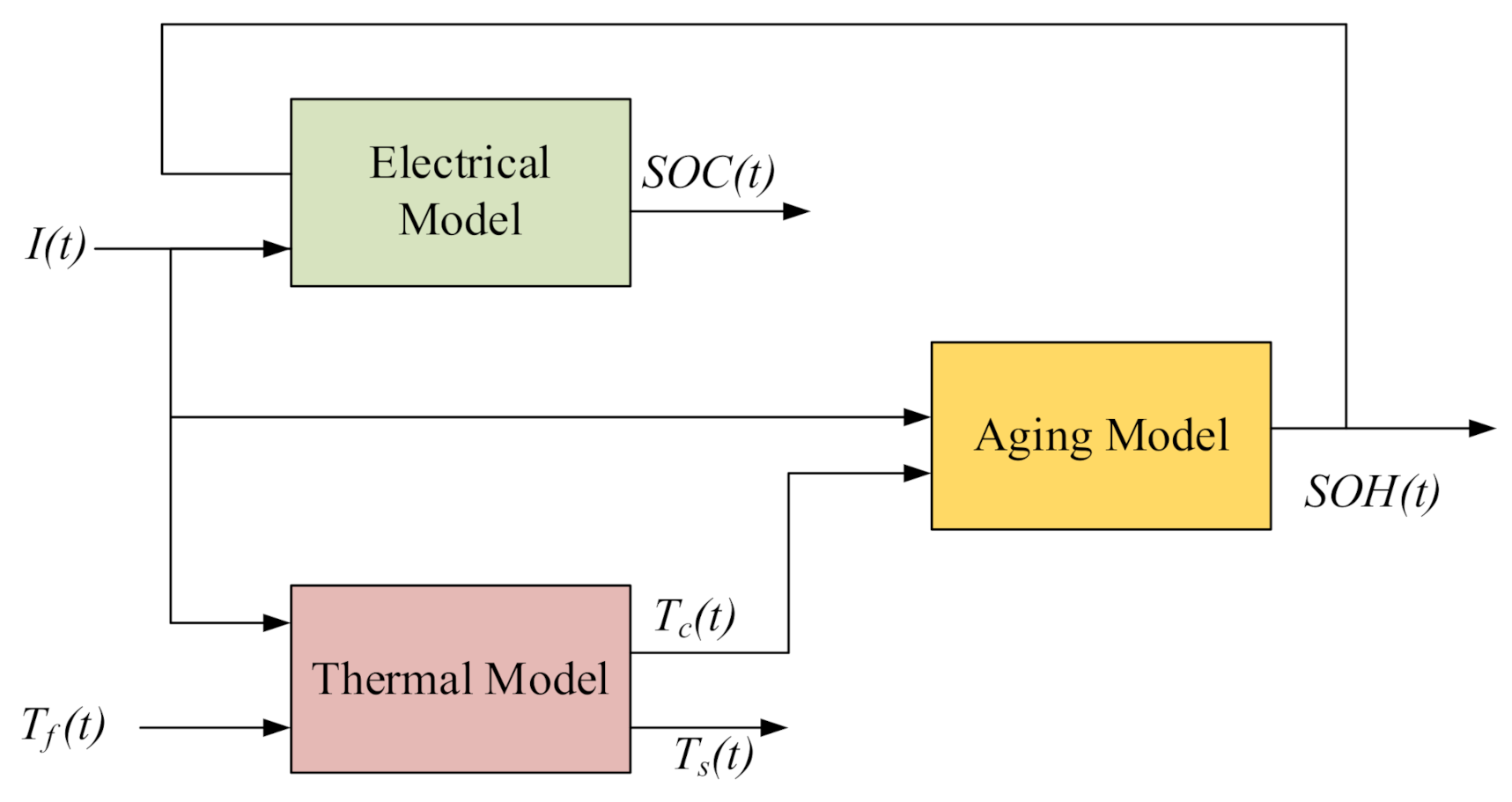
Figure 1 shows the combination of the three models. The dynamics of the model are that the inputs include the controllable current I(t), and the uncontrollable ambient temperature T_f (t).

3. Algorithms and Implementation

The Kalman filter (KF) is the broad name given to a class of stochastic estimation algorithms. However, in the strict sense, a KF refers to an estimation scheme for linear systems under the assumption of additive white noise, which follows a Gaussian distribution. Assuming that the system is stochastic in nature is truer to reality than assuming a purely deterministic process. This means that the computation is performed in a KF is accounting for variability and uncertainty within the system and attempts to supply an estimate of the optimal value, given this extra information. This stands in contrast to the deterministic observer, which uses a constant observation error gain, and does not dynamically evolve [36,37,38,39,40,41].

The assumptions made within the formulation of the KF are linear dynamics and additive Gaussian noises. Under these assumptions, properties of linear stochastic systems could be applied and neatly manipulated into an exact closed-form algorithm. As with many variants of Bayesian estimators, the algorithm for the KF is divided into two stages. The first stage is termed the model prediction/time update, where it uses a linear model with additive Gaussian process and measurement statistics to predict the next state in the time evolution of the system. Meanwhile, the second one is the measurement update that utilizes sensor measurements of the system and statistically updated “Kalman” gain to correct the model prediction estimate of the next state to the most likely value. The algorithm for the KF is shown below [42,43].

Stochastic State-Space Model:

$$x_{k+1}=A_k{x}_k+B_k{u}_k+W_k$$

$$y_k=C_k{x}_k+D_k{u}_k+v_k$$

Model Prediction:

$$x_k=A{x}_{k-1}+B{u}_k$$

$$P_k=A{P}_{k-1}{A}^T+Q$$

Measurement Update:

$$K_k=P_k{H}^T{\left(H{P}_k{H}^T+R\right)}^{-1}$$

$$x_k=x_k+K_k\left(z_k-H{x}_k\right)$$

$$P_k=\left(I-K_{k}H\right)P_k$$

3.1. Extended Kalman Filter (EKF)

The need to apply the EKF is the expected non-linearity of a true physical system. Often, in engineering practice, the knee-jerk reaction to nonlinear systems is to linearize them and hope that the resulting linearization errors prove to be insignificant. If this approach is applied to KF, the result is linearized KF (LKF). Unfortunately, the KF typically demonstrates very poor performance since it linearizes both the dynamics of the system and covariance of the system, compounding the error due to linearization. The solution is the EKF, which is an extremely important variant of the regular KF. Actually, the EKF is adapted to work with nonlinear systems while requiring a minimal change to the fundamental algorithm/processes [43].

The computing of a deterministic nonlinear equation is not easy for most users implementing state observers. In addition, the nonlinear computations are preserved and reducing linearization errors. On the other hand, nonlinear covariance and stochastic properties must be linearized since closed-form transformations of nonlinear systems are extremely challenging to solve or may not even exist. Consequently, linearization of these stochastic quantities is necessary to attempt to preserve the Gaussian of the filter, even if only an approximation. Therefore, the EKF is not an optimal observer since no guarantees of performance could be made due to the need to linearize. Finally, there exist other more advanced estimators, such as Bayesian estimator and particle filter, that could give more accurate estimation results but at a trade-off of computational expensiveness [43,44,45].

Space Model:

$$x_{k+1}=f\left(x_k,u_k\right)+w_k$$

$$y_k=\mathrm{g}\left(x_k,u_k\right)+v_k$$

where $w_k$ and $v_k$ are independent, zero-mean, Gaussian of covariance matrices, respectively.

Considering:

$$A_k=\frac{\partial f\left(x_k, u_k\right)}{\partial x}$$

$$C_k=\frac{\partial \mathrm{g}\left(x_k, u_k\right)}{\partial x}$$

For k = 1, 2, … compute:

Time Update:

$${\widehat{x}}_k^{-}=f\left({\widehat{x}}_{k-1}^{+},u_{k-1}\right)$$

$${\sum }_{\tilde{x},k}^{-}=A_{k-1}{\sum }_{\tilde{x},k-1}^{+}{A}^T{}_{k-1}+{\sum }_W$$

Measurements Update:

$$L_k={\sum }_{\tilde{x},k}^{-}{C}_k^T{\left[C_k{\sum }_{\tilde{x},k}^{-}{C}_k^T+{\sum }_v\right]}^{-1}$$

$${\widehat{x}}_k^{+}={\widehat{x}}_k^{-}+L_k\left[y_k-\mathrm{g}\left({\widehat{x}}_k^{-},u_k\right)\right]$$

$${\sum }_{\tilde{x},k}^{+}=\left(I-L_k{C}_k\right){\sum }_{\tilde{x},k}^{-}$$

3.2. State and Parameter Estimation

In the case of parameter estimation, the desired quantity to estimate is not a state of the system but some other parameter that is related to the system. In the general sense, to incorporate the desired parameter into the structure of whatever filter is being used, the parameter must be included (augmented) into the state-space model, as shown in the following form [44,45]:

$$x_{k+1}=F_k\left(p\right)x_k+G_k\left(p\right)u_k+L_k\left(p\right)w_k$$

(13)

$$y_k=H_k{x}_k+v_k$$

(14)

where $p$ is an unknown parameter vector, and by applying the following augmentation.

$$x^{\prime }=\left[\begin{array}{c}{x}_k\\ p_k\end{array}\right]$$

(15)

The system state space could be derived with parameter estimation:

$$x_{k+1}^{\prime }=\left[\begin{array}{c}{F}_k\left(p\right)x_k+G_k\left(p\right)u_k+L_k\left(p\right)w_k\\ p_k+w_{pk}\end{array}\right]$$

(16)

or:

$$x_{k+1}^{\prime }=f\left(x_k^{\prime },u_k,w_k,w_{pk}\right)$$

(17)

Additionally:

$$y_k=\left[\begin{array}{cc}{H}_k& 0\end{array}\right]\left[\begin{array}{c}{x}_k\\ p_k\end{array}\right]+v_k$$

(18)

The same algorithm used for state estimation could be implemented as estimate system parameters. It should be noted that the equation in the form given above treats the parameter as a constant value, only adding a small fictitious noise $w_{pk}$, to allow the small changes to be applied to the initial parameter value [46].

3.3. Dual Extended Kalman Filter (DEKF)

In the domain of parameter estimation with EKF, there are several approaches to achieve the same overall objective. Joint EKF runs a single filter that directly implements the augmented state-space shown above. The DEKF performs two coupled and simultaneous filters for state and parameters estimation. In general, there seems to a consensus that dual EKF demonstrates a computational advantage, while joint EKF demonstrates an accuracy advantage. For the purposes of this paper, the DEKF is implemented as the easiest solution to code and debug, where its process map has been clarified as follows [46,47,48,49,50].

State-Space Model:

$$x_{k+1}=f\left(x_k,u_k,{\theta }_k\right)+w_k \mathrm{and} {\theta }_{k+1}={\theta }_k+r_k$$

$$y_k=\mathrm{g}\left(x_k,u_k,{\theta }_k\right)+v_k \mathrm{and} d_k=\mathrm{g}\left(x_k,u_k,{\theta }_k\right)+e_k$$

where $w_k$, $v_k$, $r_k$ and $e_k$ are independent zero-mean Gaussian noise processes of covariance matrices ${\sum }_w$, ${\sum }_v$, ${\sum }_r$, ${\sum }_e$, respectively.

Definitions:

$$A_{k-1}=\frac{\partial f\left(x_{k-1},u_{k-1},{\widehat{\theta }}_k^{-}\right) }{\partial x_{k-1}}{C}_k^x=\frac{\partial \mathrm{g}\left(x_k,u_k,{\widehat{\theta }}_k^{-}\right) }{\partial x_k}{C}_k^{\theta }=\frac{d\mathrm{g}\left({\widehat{x}}_k^{-},u_k,\theta \right) }{d{x}_k}$$

Computation:

For k = +1, 2, … compute:

Weight filter time update:

$${\widehat{\theta }}_k^{+}={\widehat{\theta }}_{k-1}^{+}$$

$${\widehat{\theta }}_k^{\pm }={\sum }_{\theta ,k-1}+{\sum }_r$$

State filter time update:

$${\widehat{x}}_k^{-}=f\left({\widehat{x}}_{k-1}^{+}, u_{k-1},{\widehat{\theta }}_k^{-}\right)$$

$${\sum }_{x,k}^{-}=A_{k-1}{\sum }_{x,k-1}^{\pm }{A}^T{}_{k-1}+{\sum }_w$$

State filter measurement update:

$$L_k^x={\sum }_{\overline{x},k}^{-}{\left(C_k^x\right)}^T{\left[C_k^x{\sum }_{\overline{x},k}^{-}{\left(C_k^x\right)}^T+{\sum }_v\right]}^{-1}$$

$${\widehat{x}}_k^{+}={\widehat{x}}_k^{-}+L_k^x\left[y_k-\mathrm{g}\left({\widehat{x}}_k^{-},u_k,{\widehat{\theta }}_k^{-}\right)\right]$$

$${\sum }_{\overline{x},k}^{+}=\left(I-L_k^x{C}_k^x\right){\sum }_{\overline{x},k}^{-}$$

Weight filter measurement update:

$$L_k^{\theta }={\sum }_{\overline{\theta },k}^{-}{\left(C_k^{\theta }\right)}^T{\left[C_k^{\theta }{\sum }_{\overline{\theta },k}^{-}{\left(C_k^{\theta }\right)}^T+{\sum }_e\right]}^{-1}$$

$${\widehat{\theta }}_k^{+}={\widehat{\theta }}_k^{-}+L_k^x\left[y_k-\mathrm{g}\left({\widehat{x}}_k^{-},u_k,{\widehat{\theta }}_k^{-}\right)\right]$$

$${\sum }_{\overline{\theta },k}^{+}=\left(I-L_k^{\theta }{C}_k^{\theta }\right){\sum }_{\overline{\theta },k}^{-}$$

3.4. Sensor Estimator

The estimators utilize the measurable physical quantities, i.e., current and terminals voltage, of the cell in order to estimate its internal state. In a real application, the measurement is achieved by an acquisition unit collected by voltage and current sensors as well as single or multiple analog-to-digital converters (ADC). This ADC converts the attained analog signals into digital values. Typically, this procedure introduces a measurement noise. The estimators must be able to execute a correct estimation even in the presence of these perturbations. In order to develop reliable algorithms and to test their capability to work in an actual system, a model of the sensors has been developed.

This specified model uses the current $I$ as input during the cell voltages $V_i$ produced by the model of the battery and delivers as output. The measured current $\widehat{I}$ and voltages $\widehat{V_i}$. Both current and voltage sensors are modeled in the same way, as shown in Figure 2 and Figure 3. They introduce measurement noise as well as offset errors. Note that the mean and variance of the noise that was injected into the system were computed upon ±10%. The value of these errors is settable to simulate systems with different specifications. Furthermore, the acquisition system block can model the quantization error, i.e., the difference between the input signal value and its quantized value. This error depends on the number of bits of the ADC and its input range. These are editable parameters of the acquisition system. In particular, the current sensor input range is different from the voltage one. In fact, in this application, the voltage is a quantity included in the cell operating voltage range, which is always greater than zero. On the contrary, the current ADC has a large bipolar range.

4. Results and Discussion

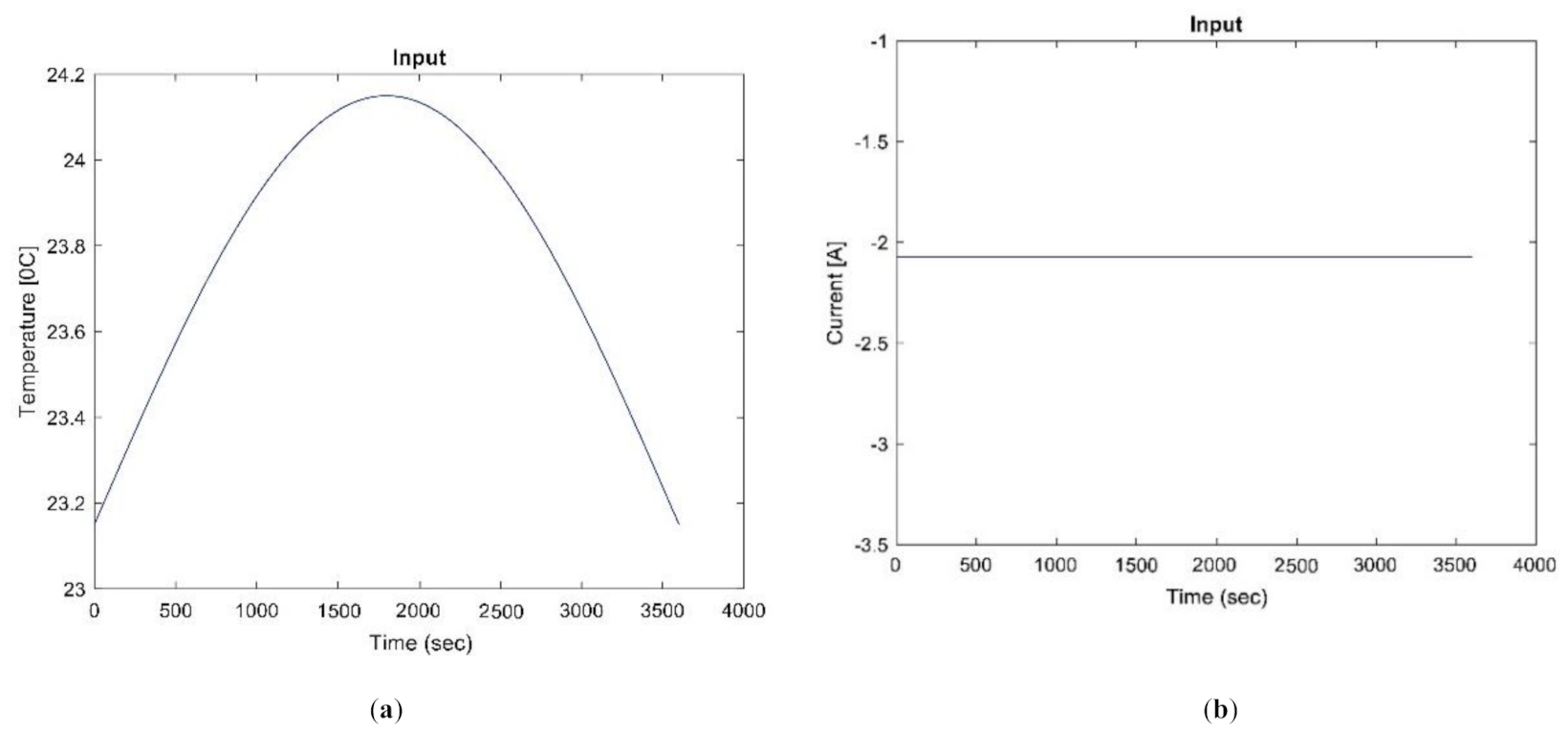
In this paper, the used parameters are based on A123 LiFePO₄ battery parameters. In the 1-h of simulation, the controllable input was the charging rate (=0.9 C-constant value). The uncontrollable one, ambient temperature, was assumed as a half-sine wave. Figure 4 presents the system inputs.

For the outputs of the simulation, after 1-h charging, the SOC reached 90%. As the SOC increased, the terminal voltage increased. As time passed, SOH decreased. Surface and core temperatures of the LiFePO₄ battery changed as they are affected by the ambient temperature and the current. Figure 5 presents these outputs.

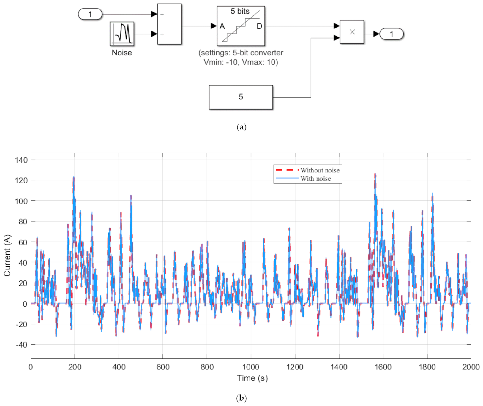
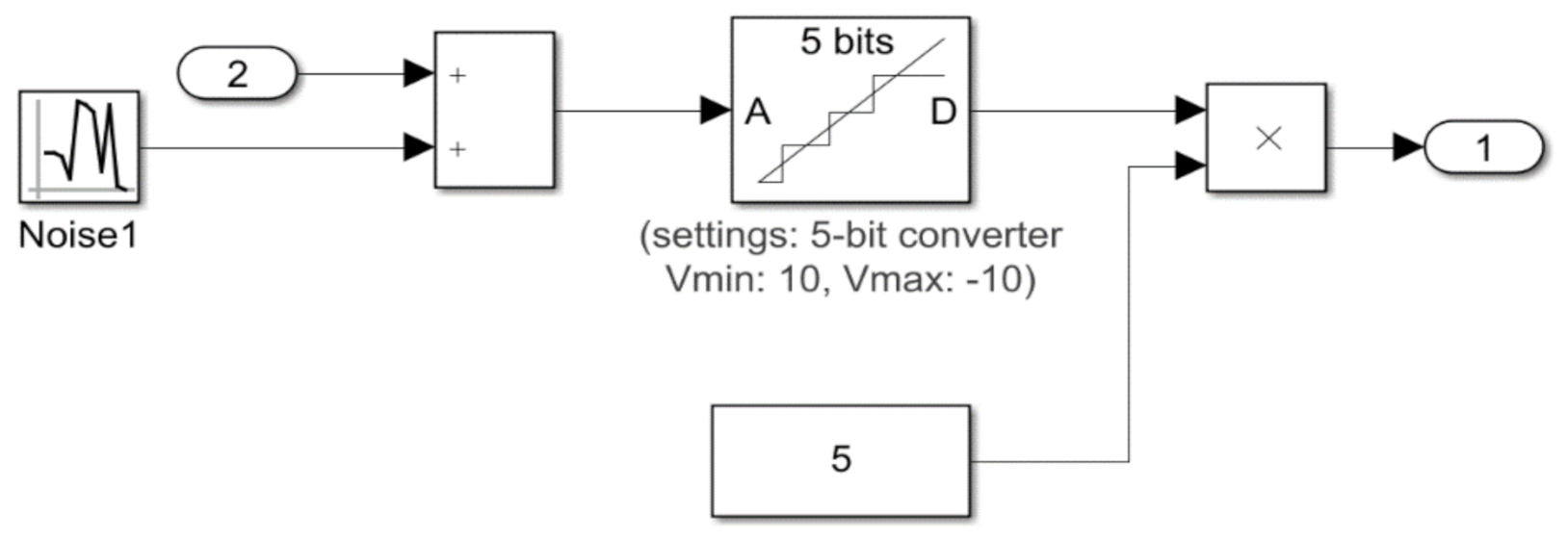
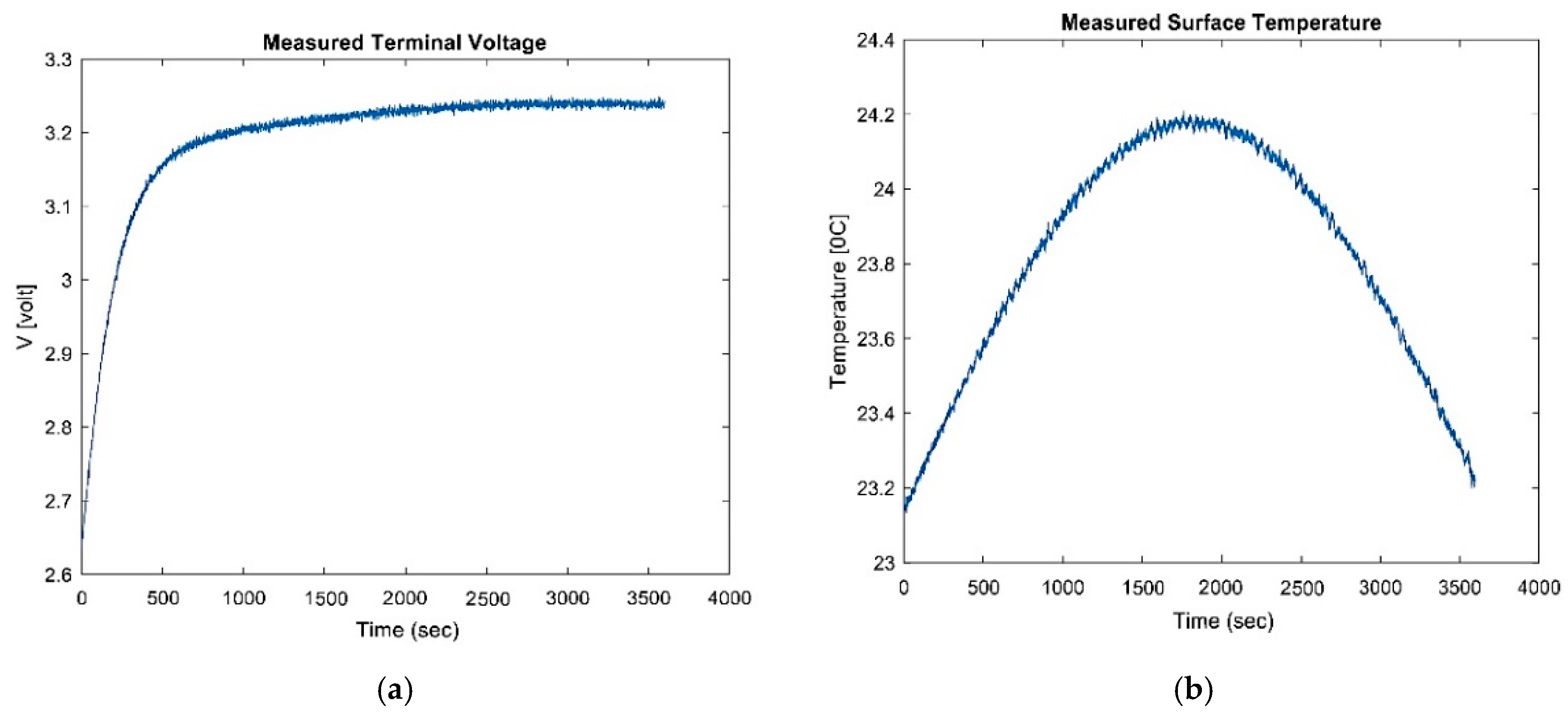
With adding white noises to both surface temperature and terminal voltage data with SNR = 60, the generated synthetic data produced surface temperature and terminal voltage measurements. Figure 6 introduces these synthetic measurements.

By using the EKF method, three different observers were created.

Table 3. The components of the three observers.

Control Inputs	Observer	Measured Inputs
Tf, Current	Temperature-measured observer	TS
Tf, Current	Voltage-measured observer	VT
Tf, Current	VT-measured observer	VT, TS

shows the three observer’s components.

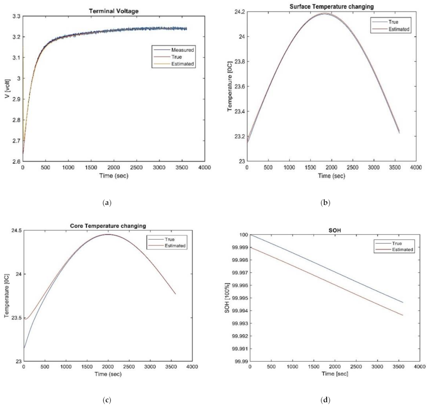
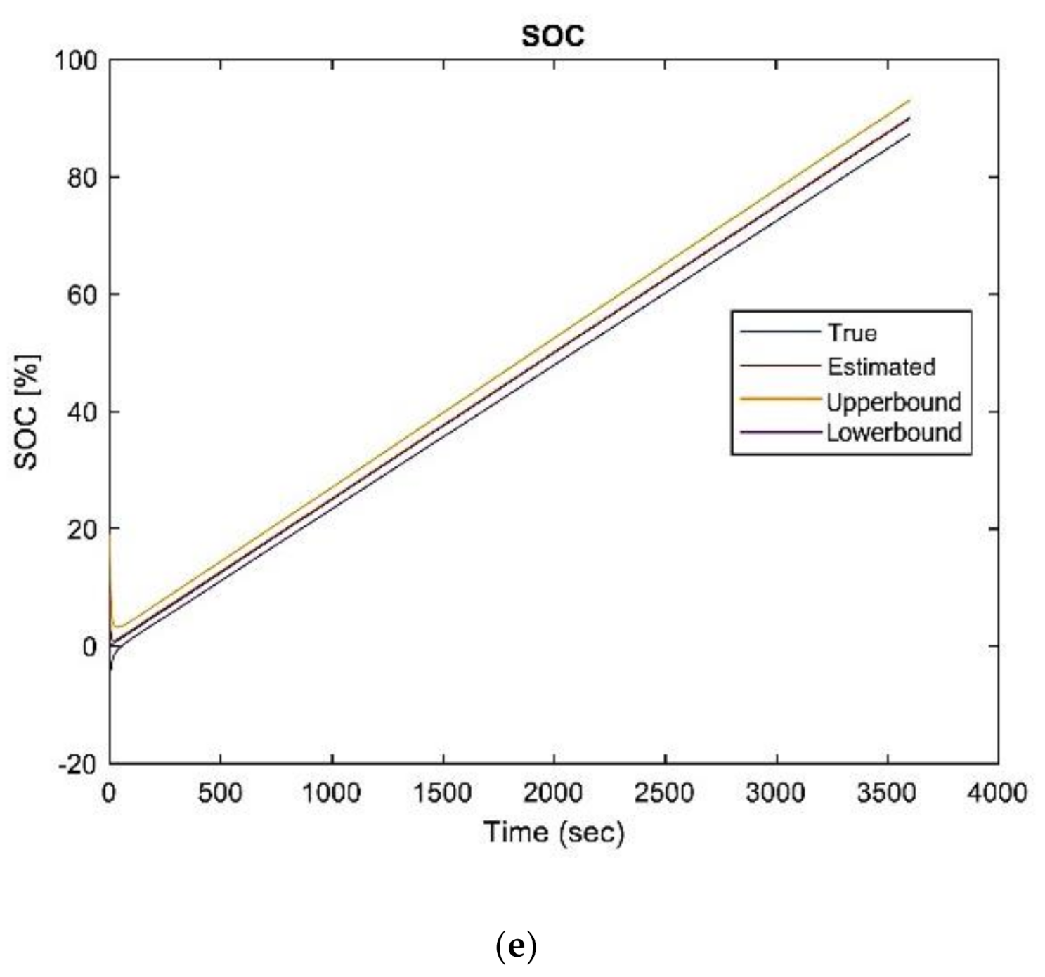
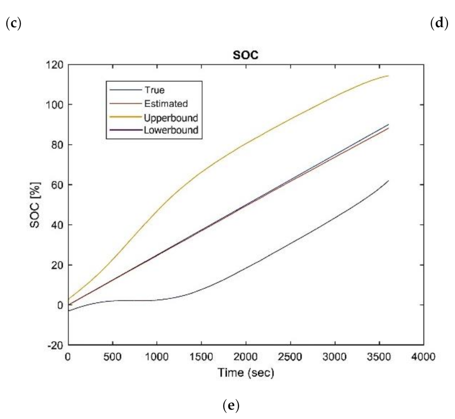
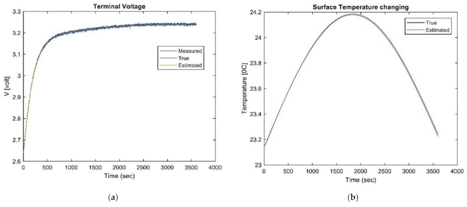
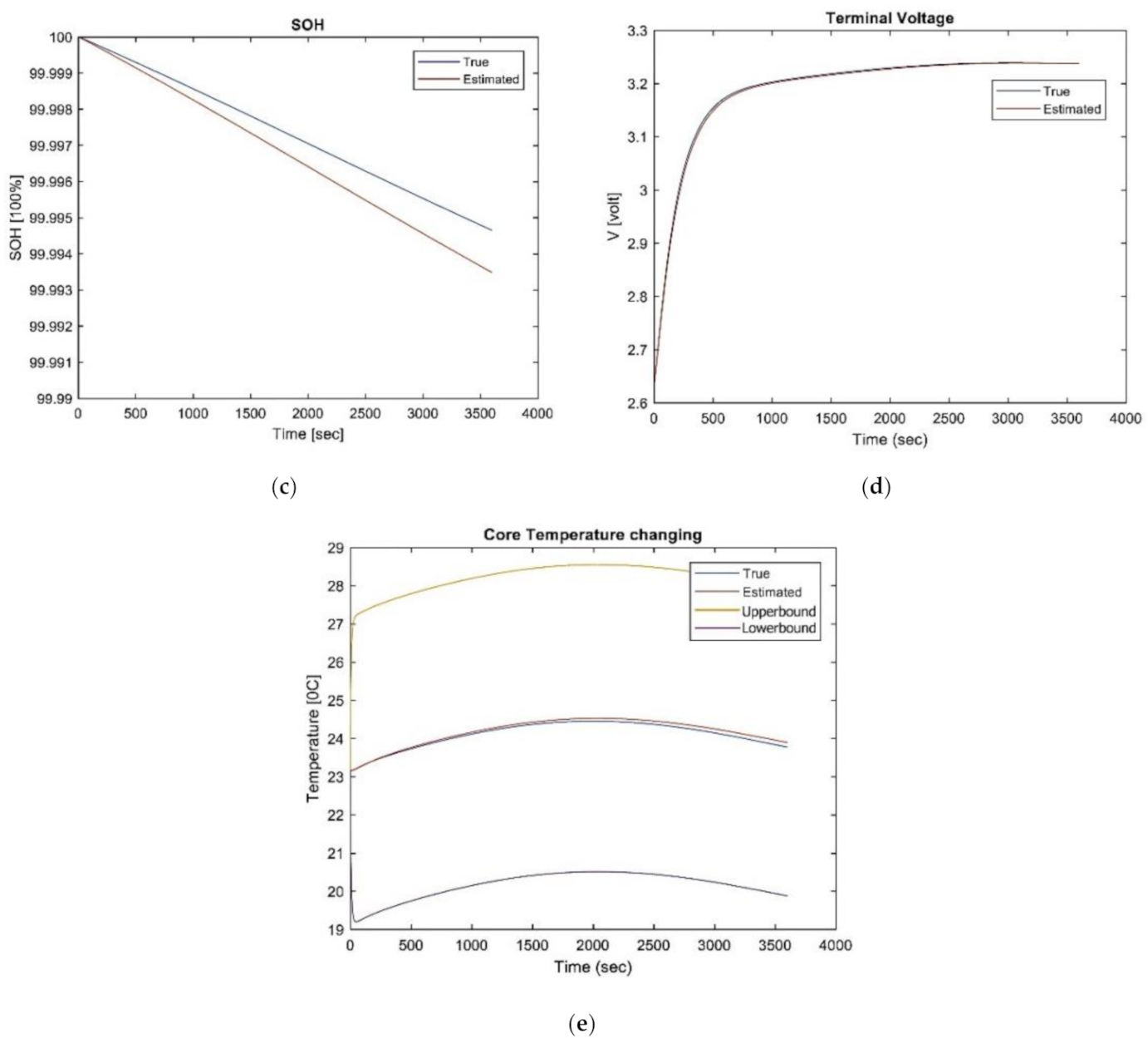
To examine the three observers’ robustness, wrong initial estimates and wrong parameter values were used, respectively. The voltage-measured observer values for that test are shown in Figure 7 and Figure 8, respectively. Note that these upper and lower bounds have been defined as the common bounds used in the literature.

Both terminal voltage and SOC were estimated well for the voltage-measured observer. After 1000 s, the estimated core and surface temperatures converged with their true values. However, that did not happen to the estimated SOH. That result indicated that the SOH was unobservable. The reason for that was that the observability matrix of the voltage-measured observer was not full rank. Span ([0, 0, 0, 1, 0, 0]^T, [0, 0, 0, 0, 1, 0]^T, [0, 0, 0, 0, 1]^T) is the observability matrix null space. That indicates that the T_c, T_s states, and SOH were unobservable. Nevertheless, when the model of the observer is accurate, the convergence of the temperatures to their true values would occur, although temperatures are unobservable for the voltage-measured observer. The reason for that is the core and surface temperatures would only reach their equilibrium states after a long time as the thermal system is asymptotically stable. 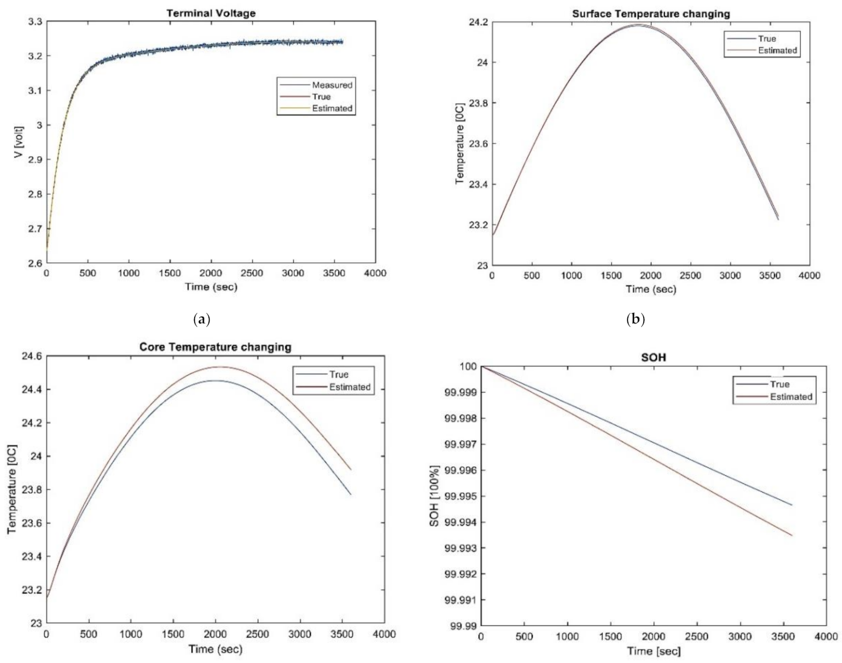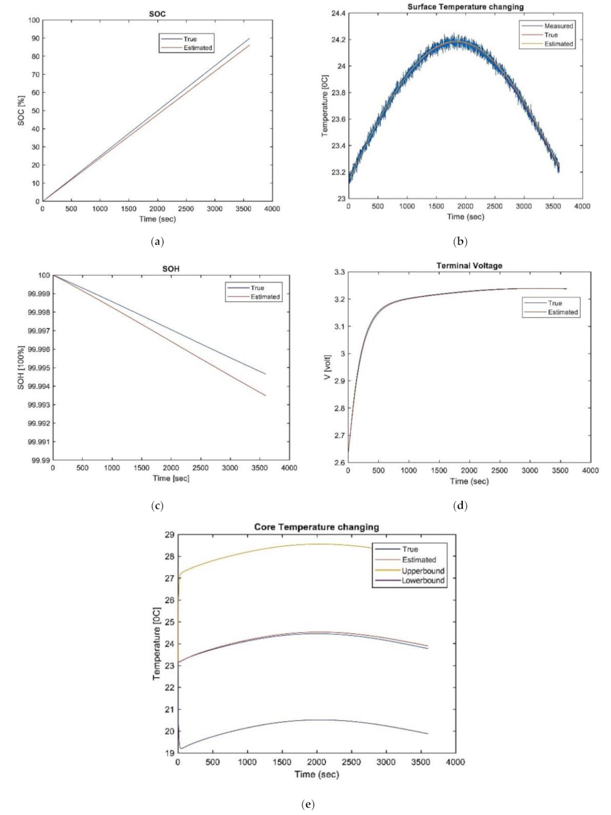Figure 9 and Figure 10 present temperature-measured observer estimation tests using wrong initial estimates and wrong parameter values, respectively.

For that observer, the core and surface temperatures are estimated well. The estimated SOC and SOH did not converge to their true values. The result of that test indicated that SOC and SOH were unobservable for that observer. The observability matrix rank of that observer was 4, which was not a full rank. Span ([1, 0, 0, 0, 0, 0]^T, [0, 0, 0, 0, 0, 1]^T) is the observability matrix null space, which indicates the unobservability of SOC and SOH for the observer as well.

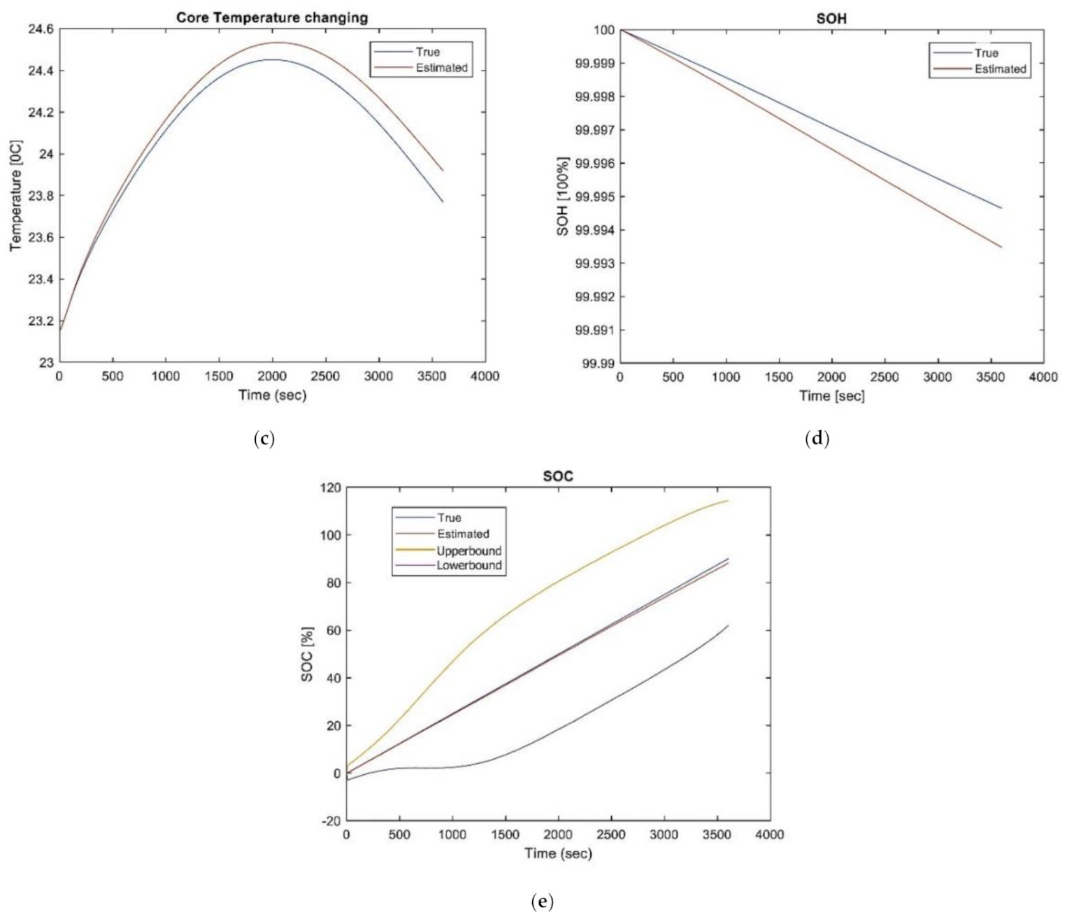
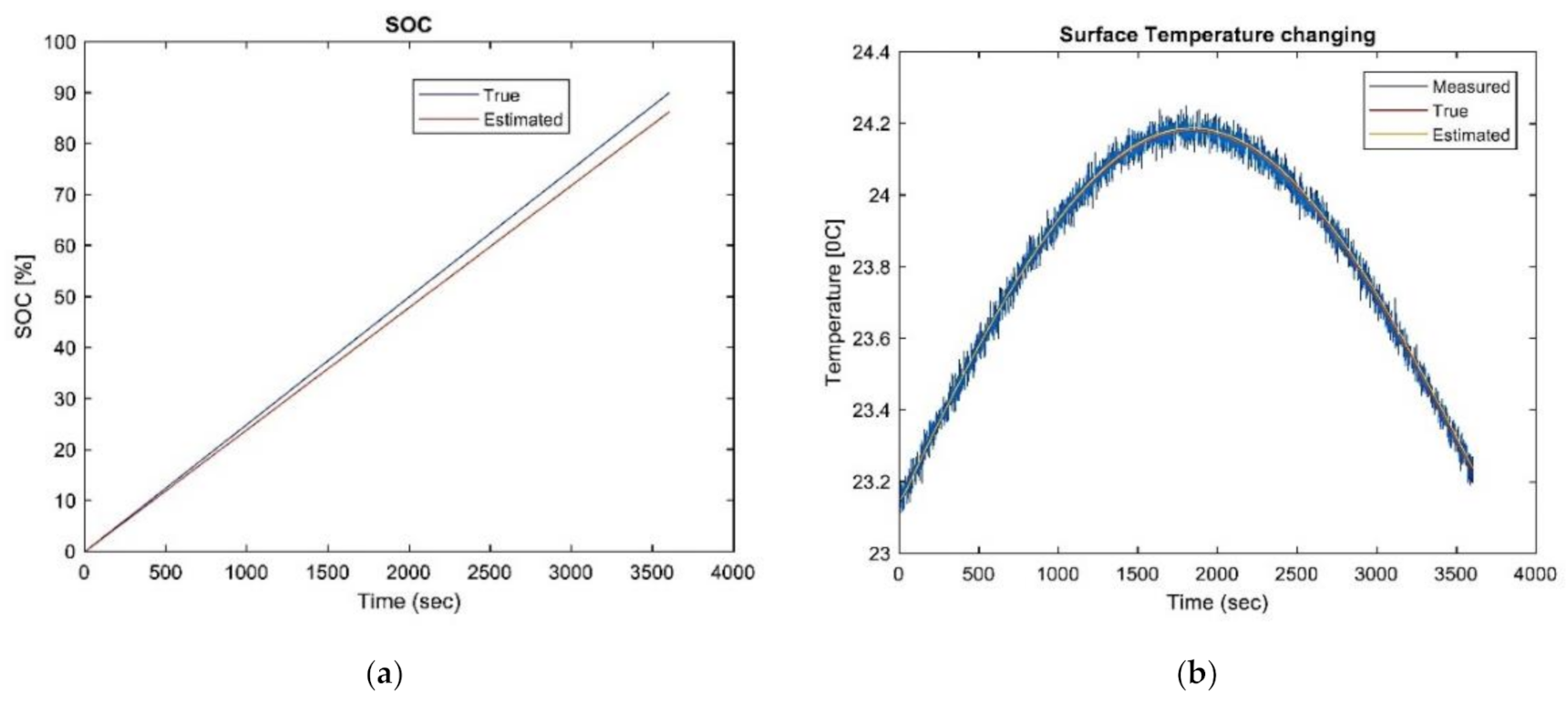
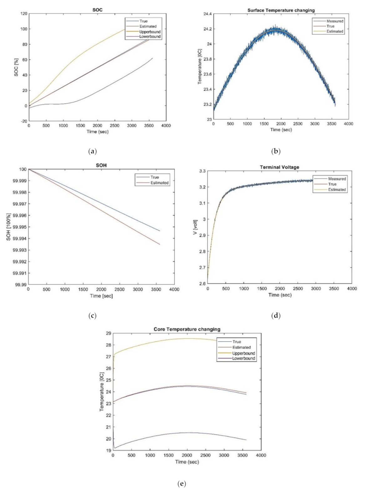
Figure 11 and Figure 12 present the results of the estimation test for the VT-measured observer using wrong initial estimates and wrong parameter values, respectively.

For the VT-measured observer, V_T, T_C, T_S, and SOC were well estimated, except for the SOH. The observability matrix rank of that observer was 5. Span ([0, 0, 0, 0, 0, 1]^T) was the observability matrix null space, which indicated the SOH unobservability as well. For the three observers’ performance evaluation, six battery states’ observability of the observers are shown in

Table 4. Observers’ observability for different states.

The Observers	SOC%	V1	V2	TS	TC	SOH%
Temperature-measured observer	No	Yes	Yes	Yes	Yes	No
Voltage-measured observer	Yes	Yes	Yes	No	No	No
VT-measured observer	Yes	Yes	Yes	Yes	Yes	No

,

Table 5. RMSE of EKF using wrong initial values.

The Observers	VT	TS	TC	SOC%	SOH%
Temperature-measured observer	0.0861	0.0055	0.0554	51.3642	0.1004
Voltage-measured observer	0.0163	0.0060	0.0607	0.2848	0.1009
VT-measured observer	0.1063	0.0059	0.0594	0.2758	0.1009

and

Table 6. RMSE of EKF using wrong parameters.

The Observers	VT	TS	TC	SOC%	SOH%
Temperature-measured observer	0.0034	0.0078	0.0798	51.4638	0.0669
Voltage-measured observer	0.0004	0.0090	0.0878	0.7590	0.0669
VT-measured observer	0.0004	0.0083	0.0848	0.7551	0.0669

, which present these three observers’ root-mean-squared error (RMSE) and two tests.

Analyzing the previous results, SOC and SOH are unobservable for temperature observers, while T_C, T_S, and SOH are unobservable for voltage observers. Nevertheless, the resistance of the circuit could affect the temperature. On the other hand, the temperature would affect the resistance as well. Therefore, T_C and T_S could be observed by an indirect approach with the voltage observer since the convergence of the temperature after a long time. That could lead to the idea that both voltage and temperature observers might be combined together as a VT-observer. Based on the results, there is an advantage for the VT-measured observer as most of the states could be estimated because it combines the two observers. It should be indicated that the SOH could not be estimated by any observer. However, the SOH values could be estimated well by an open-loop observer, provided that the model of the battery and the initial values are accurate. Additionally, based on the results, a positive linear relationship between SOC and the charging time could be noticed, while SOH has a negative one. It requires about two hours for the SOC to replenish from 0% to 90% in the simulation, with an associated SOH decay of 0.005%. The reason for running the simulation with an upper limit of 90% is to keep the health of the battery because this test will be applied many times. The lowest SOH is 99.995%, and the highest SOC is 87.4% compared to the original status. That indicates that the battery health and charging time is a tradeoff. This led to a rise in the balance between efficiency and safety. For higher efficiency, the charging time should be minimized; For the highest safety, the aging condition should be minimized. Through comparing these results with the proposed model in [29], in real-life cases, a balanced point should be found in different scenarios, which leads to a new topic—optimal control for battery charging. Since the importance of batteries as an energy storage device, the proposed observer would definitely advance sustainability. Therefore, the importance of the estimation of the states in energy systems could be noticed.

5. Conclusions

In this paper, electric, thermal, and aging models have been built, and the state estimation using DEKF and open-loop simulation has been implemented to construct an observing system for the LiFePO₄ battery. The constructive feature of the proposed observing system is that its reliable and robust performance for estimating both SOC and SOH of LiFePO₄ batteries, and so, yielding secure operation and extending their lifetime. Interestingly, the proposed open-loop observer monitors the SOC and SOH with curves’ trend as expected due to the accurate model parameters and initial values. Unlike these existing observers, the proposed VT-observer could observe the SOC, and the proposed open-loop observer could observe the SOH using correct parameters and initial estimates. The results of 1-h duration with 1-s resolutions demonstrate the reliability and robustness of the proposed observer for simultaneously monitoring the SOC and SOH of LiFePO₄ batteries.

References

1. Sánchez, L.; Anseán, D.; Otero, J.; Couso, I. Assessing the Health of LiFePO4 Traction Batteries through Monotonic Echo State Networks. Sensors 2018, 18, 9. [Google Scholar] [CrossRef] [PubMed] [Green Version]
2. Al-Gabalawy, M.; Nesreen, S.; Hosny, J.A.; Dawson, J.A.; Dawson, J.A.; Omar, A.I. State of Charge Estimation of a Li-Ion Battery Based on Extended Kalman Filtering and Sensor Bias. Int. J. Energy Res. 2021, 45, 6708–6726. [Google Scholar] [CrossRef]
3. Yin, A.; Tan, Z.; Tan, J. Life Prediction of Battery Using a Neural Gaussian Process with Early Discharge Characteristics. Sensors 2021, 21, 1087. [Google Scholar] [CrossRef] [PubMed]
4. Elsisi, M.; Tran, M.-Q.; Mahmoud, K.; Lehtonen, M.; Darwish, M.M.F. Deep Learning-Based Industry 4.0 and Internet of Things towards Effective Energy Management for Smart Buildings. Sensors 2021, 21, 1038. [Google Scholar] [CrossRef]
5. Al-Gabalawy, M. Optimal Peak Shifting of a Domestic Load Connected to Utility Grid Using Storage Battery Based on Deep Q-Learning Network. Int. J. Energy Res. 2021, 45, 3269–3287. [Google Scholar] [CrossRef]
6. Waag, W.; Fleischer, C.; Sauer, D. Critical Review of the Methods for Monitoring of Lithium-Ion Batteries in Electric and Hybrid Vehicles. J. Power Sources 2014, 258, 321–339. [Google Scholar] [CrossRef]
7. Zhang, J.; Wei, Y.; Qi, H. State of Charge Estimation of LiFePO4 Batteries Based on Online Parameter Identification. Appl. Math. Model. 2016, 40, 6040–6050. [Google Scholar] [CrossRef] [Green Version]
8. Cheng, P.; Zhou, Y.; Song, Z.; Ou, Y. Modeling and SOC Estimation of LiFePO4 Battery. In Proceedings of the 2016 IEEE International Conference on Robotics and Biomimetics (ROBIO), Qingdao, China, 3–7 December 2016; pp. 2140–2144. [Google Scholar]
9. Wang, A.; Jin, X.; Li, Y.; Li, N. LiFePO4 Battery Modeling and SOC Estimation Algorithm. In Proceedings of the 2017 29th Chinese Control and Decision Conference (CCDC), Chongqing, China, 28–30 May 2017; pp. 7574–7578. [Google Scholar]
10. Duong, V.-H.; Bastawrous, H.A.; See, K.W. Accurate Approach to the Temperature Effect on State of Charge Estimation in the LiFePO4 Battery Under Dynamic Load Operation. Appl. Energy 2017, 204, 560–571. [Google Scholar] [CrossRef]
11. Wang, Y.; You, Z.; Zhang, D.; Su, X. Characteristic Analysis and Modeling of LiFePO4Battery. In Proceedings of the 2019 IEEE Asia Power and Energy Engineering Conference (APEEC), Chengdu, China, 29–31 March 2019; pp. 234–239. [Google Scholar]
12. Mastali, M.; Foreman, E.; Modjtahedi, A.; Samadani, E.; Amirfazli, A.; Farhad, S.; Fraser, R.A.; Fowler, M. Electrochemical-Thermal Modeling and Experimental Validation of Commercial Graphite/LiFePO4 Pouch Lithium-Ion Batteries. Int. J. Therm. Sci. 2018, 129, 218–230. [Google Scholar] [CrossRef]
13. Meng, J.; Cai, L.; Stroe, D.I.; Huang, X.; Peng, J.; Liu, T.; Teodorescu, R. An Automatic Weak Learner Formulation for Lithium-ion Battery State of Health Estimation. IEEE Trans. Ind. Electron. 2021. [Google Scholar] [CrossRef]
14. Elsisi, M.; Tran, M.Q.; Mahmoud, K.; Lehtonen, M.; Darwish, M.M. Robust Design of ANFIS-Based Blade Pitch Controller for Wind Energy Conversion Systems Against Wind Speed Fluctuations. IEEE Access 2021, 9, 37894–37904. [Google Scholar] [CrossRef]
15. Mansour, D.-E.A.; Abdel-Gawad, N.M.K.; El Dein, A.Z.; Ahmed, H.M.; Darwish, M.M.F.; Lehtonen, M. Recent Advances in Polymer Nanocomposites Based on Polyethylene and Polyvinylchloride for Power Cables. Materials 2021, 14, 66. [Google Scholar] [CrossRef]
16. Alshehawy, A.M.; Mansour, D.M.; Ghali, M.; Lehtonen, M.; Darwish, M.M.F. Photoluminescence Spectroscopy Measurements for Effective Condition Assessment of Transformer Insulating Oil. Accept Processes 2021, 9. [Google Scholar]
17. Elsisi, M.; Mahmoud, K.; Lehtonen, M.; Darwish, M.M.F. An Improved Neural Network Algorithm to Efficiently Track Various Trajectories of Robot Manipulator Arms. IEEE Access 2021, 9, 11911–11920. [Google Scholar] [CrossRef]
18. Ward, S.A.; El-Faraskoury, A.; Badawi, M.; Ibrahim, S.A.; Mahmoud, K.; Lehtonen, M.; Darwish, M.M.F. Towards Precise Interpretation of Oil Transformers via Novel Combined Techniques Based on DGA and Partial Discharge Sensors. Sensors 2021, 21, 2223. [Google Scholar] [CrossRef]
19. Abouelatta, M.A.; Ward, S.A.; Sayed, A.M.; Mahmoud, K.; Lehtonen, M.; Darwish, M.M.F. Fast Corona Discharge Assessment Using FDM Integrated with Full Multigrid Method in HVDC Transmission Lines Considering Wind Impact. IEEE Access 2020, 8, 225872–225883. [Google Scholar] [CrossRef]
20. Ali, M.N.; Mahmoud, K.; Lehtonen, M.; Darwish, M.M.F. An Efficient Fuzzy-Logic Based Variable-Step Incremental Conductance MPPT Method for Grid-Connected PV Systems. IEEE Access 2021, 9, 26420–26430. [Google Scholar] [CrossRef]
21. Ali, A.; Mahmoud, K.; Lehtonen, M. Multi-objective Photovoltaic Sizing with Diverse Inverter Control Schemes in Distribution Systems Hosting EVs. IEEE Trans. Ind. Inform. 2021. [Google Scholar] [CrossRef]
22. Ali, E.S.; El-Sehiemy, R.A.; Abou El-Ela, A.A.; Mahmoud, K.; Lehtonen, M.; Darwish, M.M.F. An Effective Bi-Stage Method for Renewable Energy Sources Integration into Unbalanced Distribution Systems Considering Uncertainty. Processes 2021, 9, 471. [Google Scholar] [CrossRef]
23. Abaza, A.; El-Sehiemy, R.A.; Mahmoud, K.; Lehtonen, M.; Darwish, M.M.F. Optimal Estimation of Proton Exchange Membrane Fuel Cells Parameter Based on Coyote Optimization Algorithm. Appl. Sci. 2021, 11, 252. [Google Scholar] [CrossRef]
24. Said, M.; Shaheen, A.M.; Ginidi, A.R.; El-Sehiemy, R.A.; Mahmoud, K.; Lehtonen, M.; Darwish, M.M.F. Estimating Parameters of Photovoltaic Models Using Accurate Turbulent Flow of Water Optimizer. Processes 2021, 9, 627. [Google Scholar] [CrossRef]
25. Bendary, A.F.; Abdelaziz, A.Y.; Ismail, M.M.; Mahmoud, K.; Lehtonen, M.; Darwish, M.M.F. Proposed ANFIS Based Approach for Fault Tracking, Detection, Clearing and Rearrangement for Photovoltaic System. Sensors 2021, 21, 2269. [Google Scholar] [CrossRef]
26. Al-Gabalawy, M.; Hosny, N.S.; Hussien, S.A. Lithium-Ion Battery Modeling Including Degradation Based on Single-Particle Approximations. Batteries 2020, 6, 37. [Google Scholar] [CrossRef]
27. Kollmeyer, P.J.; Jahns, T.M. Aging and Performance Comparison of Absorbed Glass Matte, Enhanced Flooded, PbC, NiZn, and LiFePO4 12V Start Stop Vehicle Batteries. J. Power Sources 2019, 441, 227139. [Google Scholar] [CrossRef]
28. Ma, Q.; Liu, R.; Tang, C.; Wang, T.; Sun, J. LiFePO4 Battery Characteristic Analysis and Capacity Loss Prediction for Constant Current Cycling. In Proceedings of the 2019 IEEE Vehicle Power and Propulsion Conference (VPPC), Hanoi, Vietnam, 14–17 October 2019; pp. 1–5. [Google Scholar] [CrossRef]
29. Naumann, M.; Spingler, F.B.; Jossen, A. Analysis and Modeling of Cycle Aging of a Commercial LiFePO4/Graphite Cell. J. Power Sources 2020, 451, 227666. [Google Scholar] [CrossRef]
30. Zhu, M.; Hu, W.; Kar, N.C. The SOH Estimation of LiFePO4 Battery Based on Internal Resistance with Grey Markov Chain. In Proceedings of the 2016 IEEE Transportation Electrification Conference and Expo (ITEC), Dearborn, MI, USA, 27–29 June 2016; pp. 1–6. [Google Scholar] [CrossRef]
31. Guo, Q.; Qu, W.; Deng, H.; Zhang, X.; Li, Y.; Wang, X.; Yan, X. Estimation of Electric Vehicle Battery State of Health Based on Relative State of Health Evaluation. In Proceedings of the 2017 IEEE 2nd Advanced Information Technology, Electronic and Automation Control Conference (IAEAC), Chongqing, China, 25–26 March 2017; pp. 1998–2002. [Google Scholar] [CrossRef]
32. Lei, C.; Meng, J.; Stroe, D.; Peng, J.; Luo, G.; Teodorescu, R. Multi-objective Optimization of Data-driven Model for Lithium-ion Battery SOH Estimation with Short-Term Feature. IEEE Trans. Power Electron. 2020, 35, 11855–11864. [Google Scholar] [CrossRef]
33. Song, Z.; Hou, J.; Li, X.; Wu, X.; Hu, X.; Hofmann, H.; Sun, J. The Sequential Algorithm for Combined State of Charge and State of Health Estimation of Lithium-Ion Battery Based on Active Current Injection. Energy 2020, 193, 116732. [Google Scholar] [CrossRef] [Green Version]
34. Perez, H.E.; Hu, X.; Dey, S.; Moura, S.J. Optimal Charging of Li-Ion Batteries with Coupled Electro-Thermal-Aging Dynamics. IEEE Trans. Veh. Technol. 2017, 66, 7761–7770. [Google Scholar] [CrossRef]
35. Perez, H.E.; Siegel, J.B.; Lin, X.; Stefanopoulou, A.G.; Ding, Y.; Castanier, M.P. Parameterization and Validation of an Integrated Electro-Thermal Cylindrical Lfp Battery Model. In Proceedings of the ASME 2012 5th Annual Dynamic Systems and Control Conference joint with the JSME 2012 11th Motion and Vibration Conference, American Society of Mechanical Engineers, Fort Lauderdale, FL, USA, 17–19 October 2012; pp. 41–50. [Google Scholar]
36. Plett, G. Battery Management Systems; Volume I: Battery Modeling; Artech House: Norwood, MA, USA, 2015. [Google Scholar]
37. Ali, M.N.; Mahmoud, K.; Lehtonen, M.; Darwish, M.M.F. Promising MPPT Methods Combining Metaheuristic, Fuzzy-Logic and ANN Techniques for Grid-Connected Photovoltaic. Sensors 2021, 21, 1244. [Google Scholar] [CrossRef]
38. Elsisi, M.; Mahmoud, K.; Lehtonen, M.; Darwish, M.M.F. Reliable Industry 4.0 Based on Machine Learning and IoT for Analyzing, Monitoring, and Securing Smart Meters. Sensors 2021, 21, 487. [Google Scholar] [CrossRef]
39. Abbas, A.S.; El-Sehiemy, R.A.; Abou El-Ela, A.; Ali, E.S.; Mahmoud, K.; Lehtonen, M.; Darwish, M.M.F. Optimal Harmonic Mitigation in Distribution Systems with Inverter Based Distributed Generation. Appl. Sci. 2021, 11, 774. [Google Scholar] [CrossRef]
40. Bayoumi, A.S.; El-Sehiemy, R.A.; Mahmoud, K.; Lehtonen, M.; Darwish, M.M.F. Assessment of an Improved Three-Diode against Modified Two-Diode Patterns of MCS Solar Cells Associated with Soft Parameter Estimation Paradigms. Appl. Sci. 2021, 11, 1055. [Google Scholar] [CrossRef]
41. Ghoneim, S.S.; Mahmoud, K.; Lehtonen, M.; Darwish, M.M. Diagnostic Accuracy of Transformer Faults Using Teaching-Learning-Based Optimization. IEEE Access 2021, 9, 30817–30832. [Google Scholar] [CrossRef]
42. Plett, G. Battery Management Systems; Volume II: Equivalent-Circuit Methods; Artech House: Norwood, MA, USA, 2015. [Google Scholar]
43. Plett, G. LiPB Dynamic Cell Models for Kalman-filter SOC Estimation. In Proceedings of the 19th International Battery, Hybrid and Fuel Cell Electric Vehicle Symposium & Exhibition (EVS19), Busan, Korea, 19–23 October 2002. [Google Scholar]
44. Plett, G. Extended Kalman Filtering for Battery Management Systems of LiPB-Based HEV Battery Packs—Part 1: Background. J. Power Sources 2004, 134, 252–261. [Google Scholar] [CrossRef]
45. Mastali, M.; Vazquez-Arenas, J.; Fraser, R.; Fowler, M.; Afshar, S.; Stevens, M. Battery State of the Charge Estimation Using Kalman Filtering. J. Power Sources 2013, 239, 294–307. [Google Scholar] [CrossRef]
46. Wassiliadis, N.; Aderman, J.; Frericks, A.; Pak, M.; Reiter, C.; Lohmann, B.; Lienkamp, M. Revisiting the Dual Extended Kalman Filter for Battery State-of-Charge and State-of-Health Estimation: A Use-Case Life Cycle Analysis. J. Energy Storage 2018, 19, 73–87. [Google Scholar] [CrossRef]
47. Plett, G. Extended Kalman Filtering for Battery Management Systems of LiPB-Based HEV Battery Packs—Part 2: Modeling and Identification. J. Power Sources 2004, 134, 262–276. [Google Scholar] [CrossRef]
48. Plett, G. Extended Kalman Filtering for Battery Management Systems of LiPB-Based HEV Battery Packs—Part 3: State and Parameter Estimation. J. Power Sources 2004, 134, 277–292. [Google Scholar] [CrossRef]
49. Wang, L.; Lu, D.; Liu, Q.; Liu, L.; Zhao, X. State of Charge Estimation for LiFePO4 Battery via Dual Extended Kalman Filter and Charging Voltage Curve. Electrochim. Acta 2019, 296, 1009–1017. [Google Scholar] [CrossRef]
50. Kim, S.W.; Yu, J.S.; Namgoong, J.; Kim, J.H.; Kim, M.H. Progress in Li-Ion Polymer Battery and Pack System of LG Chem. For Transportation Applications. In Proceedings of the 20th Electric Vehicle Symposium (EVS20), Long Beach, CA, USA, 15–19 November 2003. [Google Scholar]
Figure 1. Electro-Thermal-Aging model coupling.
Applsci 11 03609 g001
Figure 2. Current sensor model; (a) the Matlab/Simulink block, and (b) current sensors with and without noises.
Applsci 11 03609 g002
Figure 3. Voltages sensor model.
Applsci 11 03609 g003
Figure 4. System inputs. (a) Temperature input values; (b) Current input values.
Applsci 11 03609 g004
Figure 5. Systems outputs; (a) SOC%, (b) terminal voltage, (c) SOH%, and (d) temperature changing.
Applsci 11 03609 g005
Figure 6. Measured outputs; (a) terminal voltage and (b) surface temperature.
Applsci 11 03609 g006
Figure 7. Voltage-measured observer estimation values using wrong initial values; (a) terminal voltage, (b) service temperature changing, (c) core temperature changing, (d) SOH, (e) SOC.
Applsci 11 03609 g007aApplsci 11 03609 g007b
Figure 8. Voltage-measured observer estimation test using wrong parameters; (a) terminal voltage, (b) service temperature changing, (c) core temperature changing, (d) SOH, (e) SOC.
Applsci 11 03609 g008aApplsci 11 03609 g008b
Figure 9. Temperature-measured observer estimation test using wrong initial values; (a) terminal voltage, (b) service temperature changing, (c) core temperature changing, (d) SOH, (e) SOC.
Applsci 11 03609 g009aApplsci 11 03609 g009b
Figure 10. Temperature-measured observer estimation test using wrong parameters; (a) SOC, (b) service temperature changing, (c) SOH, (d) terminal voltage, (e) core temperature changing.
Applsci 11 03609 g010aApplsci 11 03609 g010b
Figure 11. VT-measured observer estimation test using wrong initial values; (a) SOC, (b) service temperature changing, (c) SOH, (d) terminal voltage, (e) core temperature changing.
Applsci 11 03609 g011
Figure 12. VT-measured observer estimation test using wrong parameters; (a) SOC, (b) service temperature changing, (c) SOH, (d) terminal voltage, (e) core temperature changing.
Applsci 11 03609 g012