Review of Convective Heat Transfer Modelling in CFD Simulations of Fire-Driven Flows

Abstract

Progress in fire safety science strongly relies on the use of Computational Fluid Dynamics (CFD) to simulate a wide range of scenarios, involving complex geometries, multiple length/time scales and multi-physics (e.g., turbulence, combustion, heat transfer, soot generation, solid pyrolysis, flame spread and liquid evaporation), that could not be studied easily with analytical solutions and zone models. It has been recently well recognised in the fire community that there is need for better modelling of the physics in the near-wall region of boundary layer combustion. Within this context, heat transfer modelling is an important aspect since the fuel gasification rate for solid pyrolysis and liquid evaporation is determined by a heat feedback mechanism that depends on both convection and radiation. The paper focuses on convection and reviews the most commonly used approaches for modelling convective heat transfer with CFD using Large Eddy Simulations (LES) in the context of fire-driven flows. The considered test cases include pool fires and turbulent wall fires. The main assumptions, advantages and disadvantages of each modelling approach are outlined. Finally, a selection of numerical results from the application of the different approaches in pool fire and flame spread cases, is presented in order to demonstrate the impact that convective heat transfer modelling can have in such scenarios.

1. Introduction

The paper reviews the most commonly used approaches for convective heat transfer modelling in the context of fires. Focus is given on numerical modelling using Computational Fluid Dynamics (CFD) with Large Eddy Simulations (LES) considering both pool fires and turbulent wall fires (i.e., involving inert and/or combustible solid surfaces).

Progress in fire safety science, nowadays, strongly relies on the use of CFD for modelling scenarios that would be either too expensive to conduct experimentally (e.g., large-scale tests and/or performed repeatedly) or too complex, in terms of geometries, to analyse with analytical solutions and zone model approaches. Nevertheless, most real-life fire scenarios (e.g., involving industrial facilities or high-rise buildings) pose extreme challenges for CFD not only due to the different physical processes that need to be modelled (i.e., turbulence, combustion, radiation, soot, heat transfer, pyrolysis and flame spread) but also due to the wide range of length and times scales involved [1].

Boundary layer combustion [2] is a canonical configuration in fire research and applicable to various fire scenarios encountered in everyday life. A good understanding of the physics involved in such scenarios is essential and a pre-requisite for accurate and predictive fire modelling. Modelling of such scenarios (e.g., involving evaporation of liquid fuels and pyrolysis in the solid phase) can be quite challenging given the coupling between the gas and solid phases [3] which greatly affect the (convective and radiative) heat transfer to the fuel surface and the resulting fuel gasification rate [4]. The difficulties in convective heat transfer modelling lie in the fact that the convective transfer coefficient is dependant on various aspects including, e.g., the geometry of the problem (i.e., vertical, horizontal, inclined or complex surface), the type of scenario (i.e., involving natural, forced or mixed convection) as well as on the type of fluid involved (i.e., gas, liquid). Given the above mentioned aspects, no universal approach exists that can be used for modelling convective heat transfer within the context of fire scenarios. Within the context of boundary layer flows (i.e., momentum or buoyancy-driven), it is well accepted in literature that the grid sizes in the vicinity of surfaces must be millimetre-sized (i.e., values of $y^{+}\approx 1$ for wall-resolved simulations) for accurate convective heat transfer modelling [5]. On top of that, there are additional challenges involved in such scenarios including that the flows have low-to-moderate Reynolds numbers, for which the theory for turbulent boundary layers does not strictly apply, and that multi-physics phenomena (i.e., turbulence, combustion, radiation and mass transpiration) require accurate near-surface modelling.

Accurate modelling of the physical processes involved near the surface of pool fires or (flammable) walls is an active area of research in the literature [6]. When it comes to liquid pool fires, the influence of convection and radiation is often comparable for pool diameters up to $D < 0.3$ m [7,8]. The importance of convection decreases for $0.3$ m $< D < 1.0$ m until radiation becomes the dominant mode of heat transfer, with respect to the heat feedback to the fuel surface, when $D > 1.0$ m [9] due to mass transpiration effects (i.e., blockage in the convective heat fluxes due to fuel vapours leaving from the pool surface) [10]. Convection can also be important in scenarios involving flame spread, more specifically in the downstream flaming zone as well as on the early stages when pre-heating of the flammable surface occurs [11]. Recently, heat transfer modelling was also shown to greatly affect the burning behaviour of flammable walls depending on the approach used to model convection [12]. Nevertheless, the influence that convective heat transfer modelling can have in flame spread scenarios has not yet been extensively reported in literature. In general, there are still limited experimental data of individual heat flux components (i.e., convective and radiative) available for flame spread scenarios due to difficulties/uncertainties in the experimental measurements. Validation of CFD codes is then typically performed considering small-scale experiments where some experimental data are available (e.g., [13]).

The required CFD grid sizes for accurate fire plume modelling are typically in the order of centimetres [6]. Nevertheless, the required grid resolutions required within the boundary layer region (i.e., mm) for accurate convective heat transfer, even with today’s computers, can often be prohibitive for practical fire scenarios due to the wide range of length and time scales involved. In the context of LES, modelling of the boundary layer flow either involves fine-grained simulations (i.e., the flow field near the wall is well-resolved) or the use of wall functions and empirical (experimental) correlations that model the region near the wall (i.e., the flow near the wall is unresolved). An overview of these modelling approaches is presented in the paper.

2. Newton’s Law and CFD Equations

An overview of Newton’s law of cooling that governs convection as well as of the fundamental equations, typically solved by CFD codes within the context of LES, is presented in this section.

2.1. Newton’s Law of Cooling

Convection is the process of heat transfer between a surface and a fluid in motion and is governed by Newton’s law of cooling which is expressed as:

$${\dot{q}}_c^{{}^{″}}=\frac{{\dot{q}}_c}{A}=h(T_w-T_{\infty }),$$

(1)

where ${\dot{q}}_c^{{}^{″}}$ is the convective heat flux, ${\dot{q}}_c$ is the rate of convective heat transfer, A is the area where heat transfer occurs, h is the convective heat transfer coefficient, $T_w$ is the surface temperature and $T_{\infty }$ is the temperature of the surrounding fluid. The convective heat transfer coefficient, h, can be defined as the rate of heat transfer between a surface and a fluid per unit surface area per unit temperature difference.

The classification of convective heat transfer typically includes:

• Natural or free convection: fluid motion results from heat transfer and its resulting density differences (i.e., buoyancy),
• Forced convection: flow motion produced by an external agent (e.g., fan, pump),
• Mixed convection: combination of both forced and natural convection.

In general, the complexities associated with modelling convection are due to the dependency of the convective heat transfer coefficient, h, not only on the fluid properties (e.g., thermal conductivity, dynamic viscosity, density) but also on the surface geometry (e.g., horizontal, vertical) as well as on the type of flow (e.g., natural or forced convection). Typical values of the convective heat transfer coefficient encountered in different types of applications can be found

Table 1. Typical values of the convective heat transfer coefficient [14].

Application	h
	(W/(m${}^2·$ K))
Natural convection
Gases	2–25
Liquids	100–1000
Forced convection
Gases	25–250
Liquids	50–20,000

. It is worth noting that the presence of a medium is a prerequisite for convection to take place (i.e., as well as for conduction but not necessarily for radiation). Additionally, any convection scenario involves conductive heat transfer as well, occurring in a thin layer in the vicinity of the surface, since the fluid velocities there are zero (i.e., non-slip boundary condition between the fluid and the surface).

A brief overview of convective heat transfer, h, values reported in literature in the past for pool fires and flame spread scenarios, is presented below.

• Pool fires: Values in the order of $h/c_p=0.008$ kg/(m${}^2·$ s) have been reported for pools without lips while $h/c_p=0.0065$ kg/(m${}^2·$ s) for more turbulent fires with lip [15] (i.e., where $c_p=1$ kJ/(kg · K). The higher reported values for the cases without lip stem from their higher laminar heat transfer near the base of the pool [16].
• Flame spread: Under steady-state conditions, values of $h=15.9$ W/(m${}^2·$ K) have been reported by Mitler et al. [17], in the order of $h=17$–$18.2$ W/(m${}^2·$ K) by Tewarson et al. [18] while an asymptotic value of $h=18$ W/(m${}^2·$ K) was obtained from measurements conducted by Orloff et al. [15,16]. Finally, a value of $h=14$ W/(m${}^2·$ K) (i.e., a typical value corresponding to natural convection) has been used by Quintiere [19] in his modelling of the burning behaviour of PMMA. During steady-state conditions, it has been reported that radiative heat transfer accounted for approximately 75–80% [20] (or 75–87% in [21]) of the total heat fluxes in scenarios involving upward flame spread over PMM slabs. This implies that convection is expected to contribute to approximately 15–20% in the total heat transfer.

2.2. CFD Governing Equations

Within the context of fire modelling, most CFD codes (e.g., [22,23]) solve the filtered Navier–Stokes equations, along with transport equations for species mass fractions and sensible enthalpy, using Favre-filtered quantities. An overview of the main governing equations [24,25,26] (i.e., focusing on the gas phase only), often employed by CFD codes, is presented below.

• Continuity:

  $$\frac{\partial \overline{\rho }}{\partial t}+\nabla ·\left(\overline{\rho }\tilde{u}\right)=0$$

  (2)
• Momentum:

  $$\frac{\partial \left(\overline{\rho }\tilde{u}\right)}{\partial t}+\nabla ·\left(\overline{\rho }\tilde{u}\tilde{u}\right)=-\nabla \overline{p}+\nabla ·\left[{\mu }_{eff}\left(\nabla \tilde{u}+{(\nabla \tilde{u})}^T-\frac{2}{3}(\nabla ·\tilde{u})I\right)\right]+\overline{\rho }g$$

  (3)
• Chemical species:

  $$\frac{\partial \left(\overline{\rho }{\tilde{Y}}_k\right)}{\partial t}+\nabla ·\left(\overline{\rho }\tilde{u}{\tilde{Y}}_k\right)=\nabla ·\left[\overline{\rho }\left(D_k+\frac{{\nu }_{sgs}}{S{c}_t}\right)\nabla {\tilde{Y}}_k\right]+\overline{{\dot{\omega }}_k^{{}^{‴}}},(k=1,\dots ,N_s-1)$$

  (4)
• Sensible enthalpy:

  $$\frac{\partial \left(\overline{\rho }{\tilde{h}}_s\right)}{\partial t}+\nabla ·\left(\overline{\rho }\tilde{u}{\tilde{h}}_s\right)=\frac{\overline{Dp}}{Dt}+\nabla ·\left[\overline{\rho }\left(\alpha +{\alpha }_{sgs}\right)\nabla {\tilde{h}}_s\right]-\nabla ·\overline{{\dot{q}}_r^{{}^{″}}}+\overline{{\dot{q}}_c^{{}^{‴}}},$$

  (5)

  where $\rho$ is the density, u is the velocity, p is the pressure, ${\mu }_{eff}=\mu +{\mu }_{sgs}$ is the effective dynamic viscosity, $\mu$ is the molecular viscosity, ${\mu }_{sgs}=\rho {\nu }_{sgs}$ is the sub-grid scale viscosity, I is the identity tensor, g is the gravitational acceleration, $Y_k$ is the species mass fraction, $D_k$ is the species mass diffusivity, $S{c}_t$ is the turbulent Schmidt number, ${\dot{\omega }}_k^{{}^{‴}}$ is the species reaction rate, $N_s$ is the number of chemical species (i.e., typically solving for $N_s-1$ species and obtaining $N_2$ from mass conservation), $h_s$ is the sensible energy, $\alpha$ is the thermal diffusivity, $P{r}_t$ is the turbulent Prandtl number, ${\dot{q}}_r^{{}^{″}}$ is the radiative heat flux, ${\dot{q}}_c^{{}^{‴}}=\Delta H_c·{\dot{\omega }}_F^{{}^{‴}}$ is the heat release rate per unit volume due to combustion and $\Delta H_c$ is the heat of combustion of the fuel.

The sub-grid scale thermal diffusivity is calculated as:

$${\alpha }_{sgs}=\frac{{\mu }_{sgs}}{\rho P{r}_t}.$$

(6)

The assumption of a unity Lewis number is often employed by CFD codes (i.e., $Le=\alpha /D_k=1$), effectively using the effective thermal diffusivity for the diffusion in both the species (i.e., Equation (4)) and sensible energy (i.e., Equation (5)) equations. Differential diffusion effects are often neglected (i.e., $D_k=D$) since turbulent transport is more dominant than molecular diffusion for typical fire-related scenarios. Finally, the turbulent Prandtl and Schmidt numbers are also often assigned the same value (i.e., $S{c}_t=P{r}_t$).

The use of sub-models for closure of some of the terms involved in the governing equations (i.e., ${\mu }_{sgs}$ related to turbulence, $\overline{{\dot{\omega }}_k^{{}^{‴}}}$ related to combustion and $\overline{{\dot{q}}_r^{{}^{″}}}$ related to radiation) is required. Some widely-used models in fire modelling include the constant Smagorinsky [27], the dynamic Smagorinsky [28] and Deardorff [29] turbulence models, the Eddy Dissipation Model (EDM) combustion model [30] and the Finite Volume Discrete Ordinates Method (fvDOM) combined with either the constant radiative fraction approach, the grey gas model or the Weighted Sum of Grey Gas Model (WSGGM) [31] for modelling absorption/emission. A detailed presentation of these models is considered outside the scope of the paper.

The convective heat transfer models, presented later in the paper, are typically implemented in CFD codes as boundary conditions for the sub-grid scale thermal diffusivity, ${\alpha }_{sgs}$, in the sensible enthalpy equation (i.e., Equation (5)) [22]. Hence, convective heat transfer will directly influence the diffusivity of enthalpy (i.e., temperature field) in the near-field region of a surface (i.e., as well as the diffusivity of species if a unity Lewis number is employed in the modelling). The procedure through which the convective heat flux, ${\dot{q}}_c^{{}^{″}}$, is linked to the sub-grid scale thermal diffusivity, ${\alpha }_{sgs}$, is presented below.

The effective thermal diffusivity, ${\alpha }_{eff}$, is calculated based on the convective heat flux predicted from the corresponding approach as follows:

$${\alpha }_{eff}=\frac{{\dot{q}}_c^{{}^{″}}}{\rho c_p\frac{dT}{dn}},$$

(7)

where ${\alpha }_{eff}={\alpha }_{sgs}+\alpha$, $\rho$ and $c_p$ are the density and the specific heat evaluated at the surface temperature, respectively, n denotes the direction normal to the surface and $dT/dn$ is the temperature gradient based on the temperature of the first grid cell next to the surface and the surface temperature.

The sub-grid scale thermal diffusivity, ${\alpha }_{sgs}$, is then calculated by subtracting the molecular thermal diffusivity, $\alpha$, from the effective thermal diffusivity, ${\alpha }_{sgs}$, as:

$${\alpha }_{sgs}={\alpha }_{eff}-\alpha .$$

(8)

Finally, the convective heat fluxes, regardless of the method employed to estimate them, will be calculated as:

$${\dot{q}}_c^{{}^{″}}=\rho {\alpha }_{eff}{c}_p\frac{dT}{dn},$$

(9)

where the term $\rho c_p\frac{dT}{dn}$ is essentially cancelled between Equations (7) and (9).

3. Main Modelling Approaches

An overview of the main approaches, often employed by fire-related CFD codes, for modelling convective heat transfer is presented here. These approaches involve either calculation of the convective heat transfer coefficient, h, or of the convective heat fluxes, ${\dot{q}}_c^{{}^{″}}$, directly. Note that the approaches presented here can be applied to both non-reacting (i.e., not involving combustion or burning surfaces) and reacting scenarios.

Modelling of convective heat transfer, in the context of fire plume and flame spread scenarios, is a complex topic involving several modelling aspects (i.e., in both the gas and solid phases) and uncertainties for which often compensating effects are present. Isolating a specific modelling aspect (i.e., convection) in such scenarios is not possible given the inter-connected nature of all the different physical processes involved (i.e., convective heat transfer will be dependent on turbulence, combustion and radiation). The paper focuses on listing the main modelling approaches for modelling convective heat transfer reporting on possible advantages/disadvantages associated with each method. However, for the reasons mentioned above, and to avoid (potentially) drawing the wrong conclusions, the paper will not engage in a comprehensive discussion on the results available from previous numerical studies in literature.

3.1. Experimental Correlations

A typical approach for determining convective heat transfer in CFD simulations is the use of experimental (empirical) correlations based on non-dimensional numbers (i.e., the Nusselt number $Nu$) for different types of flows [32,33].

3.1.1. Non-Dimensional Numbers

Before presenting the main experimental correlations, an overview of the non- dimensional numbers involved in this approach is presented below:

• Reynolds number:

  $$Re=\frac{u{L}_c}{\nu }=\frac{\rho u{L}_c}{\mu },$$

  (10)

  expressing the ratio of inertial forces to viscous forces, is typically used to characterize whether a flow is laminar or turbulent in forced convection problems. The critical Reynolds number (i.e., number above which the flow is turbulent) varies depending on the flow configuration (e.g., $R{e}_{crit}=5\times {10}^5$ for flow over a plate) and can be used to calculate the critical distance, $x_{cr}$, from the leading edge of a surface, where the flow becomes turbulent.
• Grashof number:

  $$Gr=\frac{g\beta (T_w-T_{\infty })L_c^3}{{\nu }^2}$$

  (11)

  expressing the ratio of buoyancy forces to viscous forces, is typically used in natural convection problems.
• Prandtl number:

  $$Pr=\frac{\nu }{\alpha }=\frac{\mu c_p}{k}$$

  (12)

  expressing the ratio of molecular diffusivity of momentum to molecular diffusivity of heat across a fluid layer. The Prandtl number is used to characterize the relative thickness of the momentum and thermal boundary layers (e.g., thicker thermal boundary layer than momentum boundary layer for $Pr<1$).
• Nusselt number:

  $$Nu=\frac{h{L}_c}{k}$$

  (13)

  expressing the ratio of convective to conductive heat transfer across a fluid layer. For forced convection $Nu=f(Re,Pr)$ while for natural convection $Nu=f(Gr,Pr)$.
• Rayleigh number:

  $$Ra=Gr·Pr$$

  (14)

  expressing the ratio of buoyancy and viscosity forces multiplied by the ratio of momentum and thermal diffusivities, is typically used to characterise whether a flow is laminar or turbulent in natural convection scenarios. The critical Rayleigh number varies depending on the flow configuration and can be used to calculate the critical distance, $x_{cr}$, from the leading edge of a surface, where the flow becomes turbulent.

In the equations above, $\rho$ is the density, u is the velocity, $L_c$ is the characteristic length (to be discussed in more detail below), $\nu$ is the kinematic viscosity, $\mu$ is the dynamic viscosity, k is the thermal conductivity, $c_p$ is the specific heat and $\beta$ is the volume expansion coefficient ($\beta =1/T$ for ideal gases) of the fluid.

3.1.2. Film Temperature

The calculation of the non-dimensional numbers (i.e., $Re,Gr,Pr,Nu,Ra$) requires the evaluation of the fluid properties (e.g., $\nu$, $\alpha$, k) at a given temperature. Fluid properties are typically evaluated at the film temperature defined as [14]:

$$T_{film}=\frac{T_w+T_{\infty }}{2},$$

(15)

which is the arithmetic mean of the surface temperature (i.e., $T_w$) and the free-stream temperature (i.e., $T_{\infty }$). Within the context of CFD, $T_{\infty }$ is typically substituted by the temperature in first grid cell, $T_g$.

3.1.3. Characteristic Length $L_c$

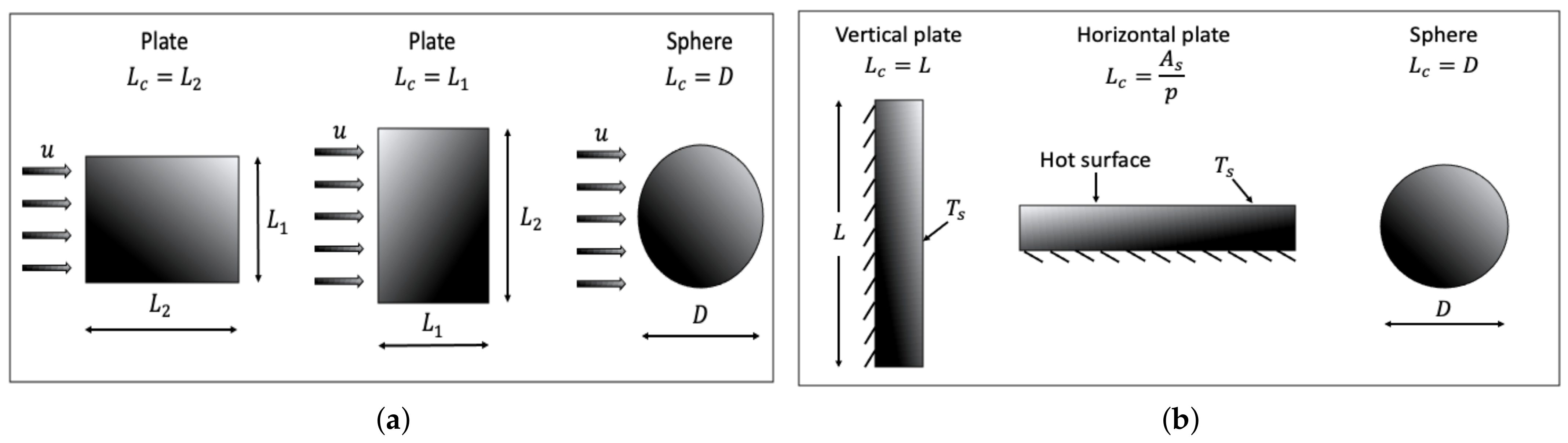
The characteristic length, $L_c$, over which convective heat transfer occurs depends on the type of scenario considered (i.e., natural or forced convection). An overview regarding the appropriate choice of $L_c$ is provided in Figure 1.

• Forced convection:
  For flow parallel to a plate: $L_c=L$ where L is the distance of the plate over which the fluid has to travel (i.e., in the direction of the flow). For flow around spheres: $L_c=D$ where D is the sphere diameter.
• Natural convection:
  For vertical plates: $L_c=L$ where L is the height of the plate. For horizontal plates: $L_c=A_s/p$ where $A_s$ and p are the surface area and perimeter of the plate, respectively. For spheres: $L_c=D$ where D is the sphere diameter.

3.1.4. Correlations

A brief overview of the most widely used experimental correlations for the Nusselt number, applicable to horizontal/vertical surfaces and spheres for both forced and natural convection scenarios, is given below. It is worth noting that these experimental correlations provide the average Nusselt number over the entire surface (i.e., use of the global characteristic length $L_c$), an approach that is most widely used in CFD modelling. No focus is given on experimental correlations based on the local Nusselt number (i.e., use of local length scales). Therefore, the non-dimensional numbers i.e., $Re$ and $Ra$ involved in

Table 2. Empirical correlations for the average Nusselt number for forced convection over isothermal surfaces. The characteristic length, $L_c$, is defined in Section 3.1.3.

Geometry	${\mathit{L}}_{\mathit{c}}$	Range of Validity	$\mathbf{Nu}$
Parallel to a plate
Laminar flow	L	$Re\le 5\times {10}^5$	$Nu=0.664R{e}^{1/2}P{r}^{1/3}$ [33]
		$0.6\le Pr\le 60$
Turbulent flow	L	$5\times {10}^5\le Re\le \times {10}^7$	$Nu=0.037R{e}^{4/5}P{r}^{1/3}$ [33]
		$0.6\le Pr\le 60$
Combined flow	L	$5\times {10}^5\le Re\le \times {10}^7$	$Nu=(0.037R{e}^{4/5}-871)P{r}^{1/3}$ [33]
		$0.6\le Pr\le 60$
Around a sphere	D	$0\le Re<200$	$Nu=2+0.6R{e}^{1/2}P{r}^{1/3}$ [35]
		$0\le Pr\le 250$

and

Table 3. Empirical correlations for the average Nusselt number for natural convection over isothermal surfaces. The characteristic length, $L_c$, is defined in Section 3.1.3.

Geometry	${\mathit{L}}_{\mathit{c}}$	Range of Validity	$\mathbf{Nu}$
Vertical plate
Laminar flow	L	${10}^4\le Ra\le {10}^9$	$Nu=0.59R{a}^{1/4}$ [32]
Turbulent flow	L	${10}^9\le Ra\le {10}^{13}$	$Nu=0.1R{a}^{1/3}$ [32]
Any type of flow	L	$Ra\le {10}^{12}$	$Nu={\left(0.825+\frac{0.387R{a}^{1/6}}{{(1+{(0.492/Pr)}^{9/16})}^{8/27}}\right)}^2$ [36]
Horizontal plate
Laminar flow	$A_s/p$	${10}^4\le Ra\le {10}^7$	$Nu=0.54R{a}^{1/4}$ [32]
Turbulent flow	$A_s/p$	${10}^7\le Ra\le {10}^{11}$	$Nu=0.15R{a}^{1/3}$ [32]
Sphere	D	Ra $\le {10}^{11}$	$Nu=2+\frac{0.589R{a}^{1/4}}{{(1+{(0.469/Pr)}^{9/16})}^{4/9}}$ [37]
		$Pr\ge 0.7$

, respectively, have to be calculated based on the characteristic length $L_c$. For completeness, a set of simplified correlations which calculate the convective heat transfer coefficients, h, in the case of natural convection is included in

Table 4. Simplified correlations for the average Nusselt number for natural convection over isothermal surfaces [34]. The characteristic length, $L_c$, is defined in Section 3.1.3.

Geometry	${\mathit{L}}_{\mathit{c}}$	Range of Validity	h
Vertical plate
Laminar flow	L	${10}^4\le Ra\le {10}^9$	$h=1.42{(\Delta T/L_c)}^{1/4}$
Turbulent flow	-	${10}^9\le Ra\le {10}^{13}$	$h=1.31{(\Delta T)}^{1/3}$
Horizontal plate
Laminar flow	$A_s/p$	${10}^4\le Ra\le {10}^9$	$h=1.32{(\Delta T/L_c)}^{1/4}$
Turbulent flow	-	${10}^9\le Ra\le {10}^{13}$	$h=1.52{(\Delta T)}^{1/3}$

. For a more complete set of empirical correlations, the reader is referred to [14,32,33,34].

The characterisation of the type of flow for forced convection (i.e., in Table 2) and for natural convection (i.e., in Table 3 and Table 4) implies the following:

• Laminar flow: The flow is laminar over the entire surface.
• Turbulent flow: The flow is turbulent over the entire surface or when the laminar region is too small relative to the turbulent region.
• Combined flow: For cases when the surface is sufficiently long for the flow to become turbulent but not long enough to disregard the laminar region.

Determination of whether the flow is laminar or turbulent is made by calculation of the Reynolds number for forced convection problems (e.g., [38]) and of the Rayleigh number for natural convection problems (e.g., [39]). Determination as to whether a combined flow exists over the surface, is made by comparing the critical distance, $x_{cr}$, (i.e., based on either the critical Reynolds or the critical Rayleigh number depending on the type of flow) with the characteristic length of the problem, $L_c$. If $x_{cr}<L_c$ then the flow over the surface is both laminar and turbulent (i.e., combined flow) while if $x_{cr}>L_c$ then the flow is laminar throughout the whole length of the surface.

The convective heat transfer, h, coefficient can be back-calculated from the Nusselt number by considering the fluid conductivity, k, and the characteristic length of the problem, $L_c$. Finally, the convective heat fluxes are then calculated based on Newton’s law as:

$${\dot{q}}_c^{″}=h(T_g-T_w),$$

(16)

where $T_g$ is the first grid cell value in the gas phase and $T_w$ is the surface temperature.

Convective heat transfer, within the context of fire-driven flows, is often modelled considering experimental correlations based on the Nusselt number [14] for either natural or forced convection. Nevertheless, there are some limitations associated with the use of such approaches, including that they have been developed for non-reacting flows, considering either iso-thermal or constant flux surfaces, and that they ignore mass transpiration effects. In addition, when employed within the context of CFD the first grid cell values are used as input in these correlations and not the free stream values since the latter are not well-defined. For this reason, the predicted rates of heat transfer can be highly dependant on the grid size [40]. It is also worth noting that uncertainties up to 25% have been reported in the resulting values of the convective heat transfer coefficient based on the free-stream properties and the roughness of the surface [14].

Both natural convection and forced convection correlations have been applied in literature in the past in order to calculate the Nusselt number and then estimate h. For example, in [41,42], it is assumed that natural convective heat transfer occurs at the surface of a burning liquid similarly to a hot surface facing upwards (see horizontal plate correlations in Table 2). On the other hand, a forced convection regime is assumed in [43]. It is of interest here to note that for natural convection, the Grashof number is proportional to the cubic power of the length scale L, i.e., $Gr\propto L^3$. Thus, $Nu\propto L^{3/4}$ in the laminar regime and $Nu\propto L$ in the turbulent regime. As h is inversely proportional to L, one obtains a −1/4 power dependence on L in the laminar regime and no dependence of h on L in the turbulent regime. A similar reasoning for the forced convection regime (where $Re$ is used) yields a −1/2 power law dependence in the laminar regime and a −1/5 power law dependence in the turbulent regime. Based on this dimensional analysis, the natural convection correlations are particularly interesting from a modelling point of view because they do not involve a length scale in the turbulent regime. This aspect would mainly be important in scenarios involving complex geometries where a single characteristic length scale would not be easily determined. In addition to the dimensional analysis, it is argued in [41] that, from a fundamental standpoint, natural convection is more representative than a forced convection with respect to the buoyancy-driven flow at the liquid surface.

Examples of modelling convective heat transfer using empirical correlation based on the Nusselt number exist in literature, e.g., [44].

3.2. Law of the Wall

This approach employs the use of wall functions [45] in order to try to mimic the sudden change of transport (i.e., from molecular to turbulent) in the vicinity of surfaces without explicitly resolving the viscous sublayer (i.e., the smallest length scales). The approach presented below is one of the available methods for modelling convective heat transfer employed by the Fire Dynamics Simulator (FDS) code [23,46]. The main theory follows dimensional analysis based on the idea that shear at the wall is constant. The friction velocity, $u_{\tau }=\sqrt{{\tau }_w/\rho }$, is an important scaling variable in the near-wall region, from which the non-dimensional streamwise velocity, $u^{+}=u/u_{\tau }$, and non-dimensional wall-normal stress distance, $y^{+}=y/{\delta }_v$, can be defined where ${\delta }_v=\nu /u_{\tau }=\mu /\left(\rho u_{\tau }\right)$ is the viscous length scale.

The law of the wall [47] for velocity can then be approximated as:

• Smooth wall:

  $$\begin{array}{c}\hfill u^{+}=y^{+}for{y}^{+}<11.81\\ \hfill u^{+}=\frac{1}{\kappa }ln\left(y^{+}\right)+Bfor{y}^{+}\ge 11.81,\end{array}$$

  (17)

  where $\kappa =0.41$ is the von K$\acute{a}$ rm$\acute{a}$n constant and $B=5.2$. The viscous and inertial stresses are important in regions (i.e., called buffer layer) where $5<y^{+}<30$. Following [48], the solution in this region is approximated by matching the viscous region and log regions at $y^{+}=11.81$.
• Rough wall:

  $$u^{+}=\frac{1}{\kappa }ln\left(\frac{y}{s}\right)+\tilde{B}\left(s^{+}\right),$$

  (18)

  where $s^{+}=s/{\delta }_v$ is the roughness length in viscous units and s is the dimensional roughness. The parameter $\tilde{B}$ can be estimated based on a piecewise function as:

  $$\tilde{B}=\left\{\begin{array}{c}B+\frac{1}{\kappa }ln\left(s^{+}\right)for{s}^{+}\ge 5.83\hfill \\ {\tilde{B}}_{max}for5.83\le s^{+}<30\hfill \\ B_{2}for{s}^{+}\ge 30,\hfill \end{array}\right.$$

  (19)

  where ${\tilde{B}}_{max}=9.5$ and the parameter $\tilde{B}$ varies with $s^{+}$ but reaches a constant value of $B_2=8.5$ in the fully rough limit [46].

By analogy to the near-wall model for velocity, the non-dimensional temperature is defined as [46]:

$$T^{+}=\frac{T_g-T_w}{T_{\tau }},$$

(20)

where $T_g$ is the gas phase temperature of the first grid cell next to the wall and the $T_w$ is the wall temperature.

The law of the wall model for $T^{+}$ is expressed as:

$$\begin{array}{c}\hfill T^{+}=Pr{y}^{+}for{y}^{+}\le 11.81\\ \hfill T^{+}=\frac{P{r}_t}{\kappa }ln\left(y^{+}\right)+B_{T}for{y}^{+}\ge 11.81,\end{array}$$

(21)

where $Pr$ and $P{r}_t$ are the molecular and turbulent Prandtl numbers, respectively.

The temperature scale, $T_{\tau }$, is defined as:

$$T_{\tau }=\frac{{\dot{q}}_c^{{}^{″}}}{\rho c_p{u}_{\tau }},$$

(22)

where ${\dot{q}}_c^{{}^{″}}$ is the convective heat flux at the wall, while $\rho$, $c_p$ and $u_{\tau }$ are the fluid density, the specific heat and the friction velocity, respectively.

The parameter $B_T$, which is the integration constant from the relation between velocity and temperature gradients, can be determined experimentally as, e.g., [49]:

$$B_T={(3.85P{r}^{1/3}-1.3)}^2+2.12 ln\left(Pr\right).$$

(23)

Finally, the convective heat transfer coefficient can then be calculated as:

$$h=\frac{{\dot{q}}_c^{{}^{″}}}{T_g-T_w}=\frac{\rho c_p{u}_{\tau }}{T^{+}}.$$

(24)

The law of the wall type of models may be more appropriate for well-resolved LES calculations in practical fire applications as they still require grid sizes that are not too coarse through evaluation of the $y^{+}$ values (i.e., the non-dimensional distance from the wall to the first mesh node).

Examples of modelling convective heat transfer using the law of the wall exist in literature, e.g., [50].

3.3. Wall-Resolved Approach

The wall-resolved approach implies the use of very fine grid sizes in order to resolve the viscous sub and transition layers (i.e., contribution from sub-grid scale quantities is zero). Within this approach, the convective heat fluxes can be calculated considering pure heat transfer by conduction (i.e., Fourier’s law) in the first grid cells as:

$${\dot{q}}_c^{″}=\rho \alpha c_p\frac{dT}{dn},$$

(25)

where $\rho$ is the density, $\alpha$ is the molecular thermal diffusivity, $c_p$ is the specific heat, n denotes the direction normal to the surface and $dT/dn$ is the temperature gradient calculated using the temperature in the first grid cell next to the wall and the wall temperature. The accuracy of the wall-resolved approach will be strongly dependant on the size of the computational grid and, typically, resolutions of the order of millimetres are needed in order to fully resolve the boundary layer. The accuracy of the convective heat transfer model has been reported to depend on the performance of the turbulence model in the near-wall region. In addition, discrepancies in the predictions of the total heat fluxes near the base of vertical flammable walls have been reported due to laminar flow structures which cannot be easily predicted by turbulence models [51].

Examples of fine-grained LES simulations of scenarios involving turbulent wall fires in literature include, e.g., [51,52,53,54], reporting on the heat feedback to the fuel surface (i.e., predicted convective and radiative heat fluxes). Additionally, an embedded flame heat flux method for simulations of quasi-steady state vertical flame spread has been reported. In this method, the convective and radiative heat fluxes during steady state were extracted from wall-resolved simulations and were used to improve the accuracy of coarse mesh simulations by embedding them as boundary conditions for the solid phase [55].

• Special case: The convective heat fluxes calculated with Equation (25) will typically start to be under-predicted with increasing grid size. To compensate for the reduction in the resolved heat fluxes, use of the effective thermal diffusivity can be made for calculating the convecting heat fluxes:

  $${\dot{q}}_c^{″}=\rho {\alpha }_{eff}{c}_p\frac{dT}{dn},$$

  (26)

  where ${\alpha }_{eff}=\alpha +{\alpha }_{sgs}$ and ${\alpha }_{sgs}$ are the effective and sub-grid scale thermal diffusivities, respectively. This approach considers sub-grid scale effects and attempts to model the convective heat transfer coefficient, h, without the explicit need of an empirical correlation through the use of a turbulence model.

The accuracy of this modelling approach will be dependant on the employed grid size as well as on the performance of the turbulence model near the wall. Ideally, the turbulence model should be able to predict vanishing turbulence close to the surface and to capture transitions from laminar to turbulent flows. Capturing these modelling aspects with turbulence models using constant coefficients will be more challenging as opposed to dynamic turbulence models. Towards the DNS limit, the sub-grid scale thermal diffusivity would tend to zero in this case and any heat transfer would be by pure conduction (i.e., Fourier’s law). This requirement will be satisfied by the dynamic Smagorinsky model, since the model parameter will tend to zero as the grid size approaches the Kolmogorov length scale, in contrast to the Smagorinsky model using a constant coefficient which will introduce a fixed error [56].

A convective heat transfer model, based on the concept of the effective thermal diffusivity, with a correction of the convective fluxes at coarse grids was recently reported in literature [11]. Additionally, the model has been applied to model convective heat transfer in upward flame spread of Single Burning Items (SBI) scenarios [12].

4. Specific Treatment of Burning Surfaces

In this section, the analogy between convective heat transfer and convective mass transfer is briefly outlined. In addition, an analysis of the additional aspects that need to be considered in scenarios involving simultaneously heat and mass transfer is given and an overview of different approaches specifically developed for modelling convective heat transfer of burning surfaces is presented. Finally, selected CFD results from the application of different modelling approaches for modelling convective heat transfer in pool fire and flame spread scenarios are presented.

4.1. Convective Mass Transfer: Analogy with Convective Heat Transfer

The dimensionless number involved in mass transfer problems, equivalent to the Nusselt number for heat transfer, is the Sherwood number defined as:

$$Sh=\frac{h_m{L}_c}{D},$$

(27)

expressing the ratio of the convective mass transfer to the rate of diffusive mass transport across a fluid layer. In the equation above, $h_m$ is the convective mass transfer coefficient, $L_c$ is the characteristic length of the problem and D is the mass diffusion coefficient.

Additionally, the Schmidt number (i.e., equivalent to Prandtl number in heat transfer) is defined as:

$$Sc=\frac{\nu }{D}=\frac{\mu }{\rho D},$$

(28)

expressing as the ratio of momentum diffusivity and mass diffusivity. The $Sc$ number is used to characterise fluid flows in which simultaneous momentum and mass diffusion processes occur.

Since $Pr\approx Sc\approx 0.7$ for combustion gases, then $Le=Pr/Sc\approx 1$ and it can be shown that $h_m=h/c_p$. This way, the mass transfer coefficient can be computed from heat transfer results (i.e., it stems from the Reynolds analogy which relates heat and mass transfer when $Le\approx 1$). The mass transfer coefficients, $h_m$, for forced convection problems can be obtained from Table 2 with the Prandtl number, $Pr$, replaced by the Schmidt number, $Sc$, and the Nusselt number, $Nu$, replaced by the Sherwood number, $Sh$ (i.e., $Sh=f(Re,Sc)$ ). An overview of these correlations is presented in

Table 5. Empirical correlations for the average Sherwood number for forced convection over surfaces. The characteristic length, $L_c$, is defined in Section 3.1.3.

Geometry	${\mathit{L}}_{\mathit{c}}$	Range of Validity	Sh
Parallel to a plate
Laminar flow	L	$Re\le 5\times {10}^5$	$Sh=0.664R{e}^{1/2}S{c}^{1/3}$ [33]
		$0.6\le Sc\le 60$
Turbulent flow	L	$5\times {10}^5\le Re\le \times {10}^7$	$Sh=0.037R{e}^{4/5}S{c}^{1/3}$ [33]
		$0.6\le Sc\le 60$
Combined flow	L	$5\times {10}^5\le Re\le \times {10}^7$	$Sh=(0.037R{e}^{4/5}-871)S{c}^{1/3}$ [33]
		$0.6\le Sc\le 60$
Around a sphere	D	$0\le Re<200$	$Sh=2+0.6R{e}^{1/2}S{c}^{1/3}$ [35]
		$0\le Sc\le 250$

.

Alternatively, use can also be made of experimental correlations for the Sherwood number [9] derived from burning surfaces. A brief overview of some, typically used, correlations in literature is presented below.

• Natural convective burning over vertical plates [57]:

  $$Sh=\frac{{\dot{m}}^{{}^{″}}{c}_p{L}_c}{k}=\frac{0.66R{a}_{*}^{1/4}}{\Sigma P{r}^{3/4}},R{a}_{*}\le {10}^9\left(Laminarflow\right)$$

  (29)

  $$Sh=\frac{{\dot{m}}^{{}^{″}}{c}_p{L}_c}{k}=\frac{0.0284R{a}_{*}^{0.4}}{\Sigma P{r}^{2/3}},R{a}_{*}>{10}^9\left(Turbulentflow\right)$$

  (30)

  with

  $$G{r}_{*}=\left(\frac{L_v}{4c_p{T}_{\infty }}\right)\left(\frac{g{L}^3}{{\nu }^2}\right)$$

  (31)

  $$\Sigma ={\left[\frac{1+B}{ln(1+B)B}\right]}^{1/2}{\left[\frac{1+0.5Pr/(1+B)}{3(B+{\tau }_o)\eta +{\tau }_o}\right]}^{1/4}$$

  (32)

  $${\tau }_o=\frac{c_p(T_{ign}-T_{\infty })}{L_v}$$

  (33)

  $$\eta =1-{\theta }_{FO}^{1/3}$$

  (34)

  $${\theta }_{FO}=\frac{r_o(B+1)}{B(r_o+1)}$$

  (35)

  $$r_o=\frac{Y_{O_2,\infty }}{r{Y}_{F,o}}$$

  (36)

  $$B=\frac{Y_{O_2,\infty }\Delta H_{O_2}-c_p(T_{ign}-T_{\infty })}{L_v},$$

  (37)

  where $R{a}_{*}=G{r}_{*}·Pr$ is a modified Rayleigh number, $L_v$ is the latent heat of vaporization of the fuel, $\nu$ is the kinematic viscosity, $Y_{F,o}$ is the mass fraction of the fuel, $O_{2,\infty }$ is the oxygen mass fraction in ambient air and r is the stoichiometric mass oxygen to fuel ratio.
• Forced convective burning of a flat plate [58]:

  $$Sh=\frac{{\dot{m}}^{{}^{″}}{c}_p{L}_c}{k}=0.385{\frac{u{L}_c}{\nu }}^{1/2}Pr\frac{ln(1+B)}{B^{0.15}}$$

  (38)

  where u is the flow velocity, $\nu$ is the kinematic viscosity of the fluid and B is the B-number of the fuel.

4.2. Blowing Effect

In fire scenarios (e.g., related to pool fires and flame spread) which involve simultaneously both convective heat and mass transfer, consideration of mass transpiration effects (i.e., ‘blowing’ effect) has to be made. This correction (i.e., blocking) factor, applied to the calculation of the convective heat fluxes, represents a reduction in the heat transfer process as mass transfer increases (e.g., release of flammable fuel vapours in liquid pool fires or combustible solid surfaces) and can be calculated as [9]:

$$f_{blowing}=\frac{(c_p·{\dot{m}}^{″})/h}{exp[(c_p·{\dot{m}}^{″})/h]-1},$$

(39)

where $c_p$ is the specific heat of the fluid, h is the convection coefficient and ${\dot{m}}^{″}$ is the fuel mass loss rate per unit area. The parameter $f_{blowing}$, which varies between 0 and 1 (i.e., approaches 1 as ${\dot{m}}^{″}\to 0$), acts to enlarge the boundary layer, due to blowing caused by the vaporized fuel, making it difficult to transfer heat across it [9]. For a detailed derivation of Equation (39) the reader is referred to [9].

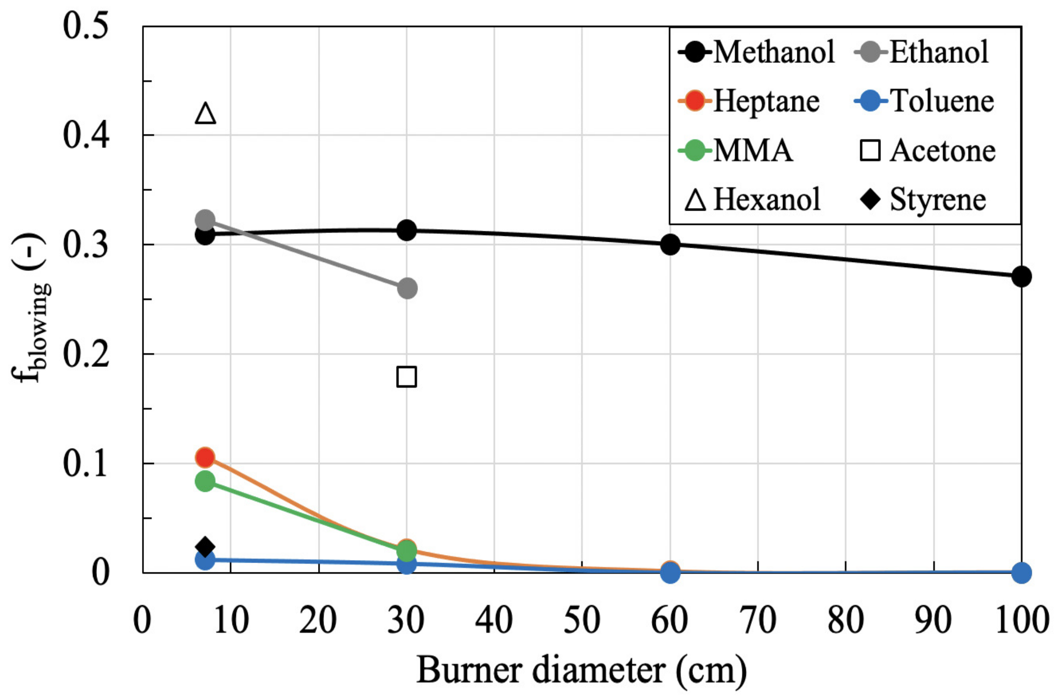
Figure 2 presents the magnitude of the $f_{blowing}$ factor for several fuels (i.e., both sooty and non-sooty) and pool diameters (i.e., 7 cm–100 cm). The experimental data are taken from [59,60] while a value of $h/c_p=0.0065$ kg/(m${}^2·$ s) for turbulent lip fires [15] has been considered. The results, as expected, suggest that for sootier fuels (e.g., toluene) and for increasing burner diameters, the blowing factor values decrease (i.e., significant blockage of convective heat towards the fuel surface).

The effect of mass transpiration (i.e., blockage of convective heat transfer with increasing mass transfer rates) has been reported experimentally in the past for upward spread scenarios over vertical PMM slabs [20]. Additionally, the inclusion of mass transpiration effects has also been considered when modelling flame spread using the approaches based on the law of the wall (e.g., [50]), based on the stagnant film theory (e.g., [12]) as well as on the convective heat transfer model of FireFOAM 2.2.x (e.g., [61,62,63]).

4.3. Modelling Approaches

An overview of approaches related to convective heat transfer modelling which are applicable when burning surfaces are involved, and that have appeared in the literature in the past, are presented in this section. The modelling approaches, previously presented in Section 3, are also applicable here even though not explicitly developed for flows involving burning surfaces.

• Based on the stagnant film theory [15,16]:
  The model is based on a 1D steady stagnant film approach and describes the gas-phase combustion process by considering known heat transfer relationships. The convective heat fluxes can be calculated as [9]:

  $${\dot{q}}_c^{″}=\frac{h}{c_p}\left[\left(\frac{{\chi }_a-{\chi }_r}{{\chi }_a}\right)Y_{O_2,\infty }\Delta H_{O_2}-c_p(T_w-T_{\infty })\right]·f_{blowing},$$

  (40)

  where ${\chi }_a$ is the combustion efficiency of the fuel, ${\chi }_r$ is the (global) radiative fraction, $Y_{O_2,\infty }$ is the ambient oxygen mass fraction, $\Delta H_{O_2}$ is the heat of combustion per kg of $O_2$ consumed (i.e., approximately 13.1 MJ/kg for many hydrocarbon fuels), $c_p$ is the heat capacity, $T_w$ is the surface temperature which, in a fully developed fire, can be taken as the boiling point for a liquid or the ignition temperature for a solid, $T_{\infty }$ is the ambient temperature and $f_{blowing}$ is a correction for the ‘blowing’ effect (i.e., see Section 4.2). This expression stems from the classical B-number theory which describes liquid fuel evaporation due to convective heat transfer from nearby flames [9]. Estimation of the convection coefficients, h, can be made through the use of empirical experimental correlations based on the Nusselt number (e.g., Table 2 and Table 3). The calculation of the convective heat fluxes based on the stagnant film theory does not involve the flame temperature directly (i.e., Equation (40)) rather only indirectly through the temperature-dependent properties (e.g., convection coefficient h, heat capacity $c_p$, thermal conductivity k, and Prandtl number $Pr$). For a detailed derivation of Equation (40) the reader is referred to [9]. It is interesting to note that Equation (40) can be re-written as:

  $${\dot{q}}_c^{″}=h(T_f-T_s),$$

  (41)

  where $T_f$ is a global flame temperature calculated as:

  $$T_f=T_{\infty }+\left(\frac{({\chi }_a-{\chi }_r)\Delta H_{O_2}}{{\chi }_a{c}_p}\right)\left(\frac{Y_{O_2,\infty }\Delta H_{O_2}}{c_p}\right).$$

  (42)
  The concept of a global flame temperature is further discussed, in the context of liquid pool fires, in [42].
  Employing the stagnant film theory for modelling convective heat transfer has been considered in literature in the past e.g., for predicting the mass loss rates of pool fires (e.g., [16,42]), for determining the convective heat fluxes from pool fire experiments (e.g., [64]) and in numerical simulations involving liquid pool fires in mechanically ventilated compartments (e.g., [65,66]). The method based on stagnant film theory, previously shown to be both accurate and grid insensitive for pool fires [67], has had limited applicability on CFD simulations of flame spread until recently, e.g., [12] but has been employed in a global analytical model [68] for determining the convective heat feedback from the gas-phase combustion to the surface of charring materials.
• FireFOAM 2.2.x model:

  -

  If ${\dot{m}}_{pyrol}^{″}<{10}^{-4}$ kg/(m${}^2·$ s):

  $${\dot{q}}_c^{″}=\frac{min(max(0,{\dot{q}}_{c,laminar}^{″}),{\dot{q}}_{c,threshold}^{″})}{{\dot{q}}_{c, threshold}^{″}}{\dot{q}}_{c, flame}^{″}$$

  (43)

  -

  If ${\dot{m}}_{pyrol}^{″}\ge {10}^{-4}$ kg/(m${}^2·$ s):

  $${\dot{q}}_c^{″}={\dot{q}}_{c, flame}^{″}·f_{blowing},$$

  (44)

  where ${\dot{m}}_{pyrol}^{″}$ is the mass loss rate due to pyrolysis of the solid fuel, ${\dot{q}}_{c, laminar}^{″}=-\alpha \rho c_p\frac{\partial T}{\partial s}$ is the convective heat flux calculated based on the molecular thermal diffusivity (positive for heating up of the wall, i.e., $T_g > T_w$), s is the direction normal to the wall, ${\dot{q}}_{c, threshold}^{″}$ is a threshold value (e.g., in the range of $0.5$ kW/m ${}^2$ [61]), ${\dot{q}}_{c, flame}^{″}$ is the maximum value (e.g., in the range of $15$ kW/m ${}^2$ [61]) of the convective heat flux without mass transfer (i.e., calculated based on an average temperature difference and a convection coefficient value) and $f_{blowing}$ is a correction for the ‘blowing’ effect (i.e., see Section 4.2). This approach, does not directly take into account the local properties of the flow and considers that the convective heat fluxes remain relatively constant with elevation (i.e., the convective heat transfer coefficient, h, is not calculated). The first part of the wall function is employed in the early stages of flame spread when pre-heating of the virgin material occurs and there is no (substantial) burning. In this case, a linear function will assign a fraction of the a priori-determined convective heat flux in the fuel surface based on the fire intensity (i.e., determined by the resolved convective heat flux) in this area [61,62].

  The convective heat transfer approach used in FireFOAM 2.2.x has some deficiencies. More specifically, a constant ${\dot{q}}_{c, flame}^{″}$ value is employed and the convective heat fluxes only change due to mass transpiration effects, not directly accounting for local properties of the flow (i.e., in the determination of the ${\dot{q}}_{c, flame}^{″}$). Effectively, the main part of the convective heat transfer model (i.e., Equation (43)) does not explicitly consider the flame temperature for determining the convective heat transfer value, since ${\dot{q}}_{c, flame}^{″}$ is an a-priori determined value, rather it is only used for calculating ${\dot{q}}_{c, laminar}^{″}$.

  Examples of modelling convective heat transfer using this approach exist in literature when it comes to flame spread over large-scale configurations, e.g., [62,63].

4.4. Special Topic: Convective Heat Transfer within the Liquid

When computing the convective heat flux at the liquid surface, besides the convective heat transfer coefficient, h, and the gas phase temperature, $T_g$, the liquid surface temperature is required. In general, when steady-state in fully-developed conditions is considered, the surface temperature is generally taken as the boiling temperature of the liquid. However, when transient calculations are sought, the surface temperature is calculated using a heat balance, which, in the most advanced approach, is coupled to the convective motion of the liquid by solving the Navier-Stokes equations as in e.g., [69,70].

The convective motion of the liquid may be caused by several mechanisms which, most likely, occur simultaneously. The first mechanism is due to the non-uniform heat flux distribution at the surface of the liquid which yields a non-uniform surface temperature distribution and consequently surface tension gradients therein. The liquid moves then from low surface tension regions to high surface tension regions. This is known as the Marangoni or capillary effect. The convective motion of the liquid may also be caused by a temperature difference between the liquid and the burner walls. A third potential cause for liquid motion is in-depth radiation, which causes the liquid temperature slightly beneath the surface to be higher than the surface temperature. This results in a hydrodynamic instability (called the Rayleigh-B$\acute{e}$nard instability), making the hot liquid rise above the slightly less hot liquid.

Detailed experimental data on the convective motion of the liquid in a pool fire remain very scarce. To the best of our knowledge, the most comprehensive experimental work on this topic has been carried out by Vali and his co-workers (e.g., [71]) where the flow field within the liquid has been measured using PIV and the thermal structure (of the liquid) has been characterised using thermocouples. However, the work remained limited to a 9 cm-diameter methanol pool fire.

From a modelling perspective, solving the Navier-Stokes equations, as done by Fukumoto et al. [69], remains a very computationally intensive approach for ‘practical’ fire dynamics simulations where a lot of resources are mainly devoted to the gas phase, given its importance with respect, for example, to tenability and structural integrity. The most common approach is to treat the liquid as a ‘thermally-thick solid’ by solving a 1D Fourier’s equation. In [43], convective motion of the liquid and the subsequent increased heat-up are indirectly accounted for by using the ‘effective thermal conductivity’, $k_{eff}$, which is calculated as:

$$k_{eff}=N{u}_i·k,$$

(45)

where k is the actual thermal conductivity of the liquid and $N{u}_i$ is the ‘internal’ Nusselt number (within the liquid), not to be confused with the Nusselt number used for convective heat transfer at the interface between the liquid and the surrounding gas.

In [43], $N{u}_i$ is calculated from a correlation for internally heated horizontal plane layer with isothermal top boundary and thermally insulated bottom boundary:

$$N{u}_i=0.338R{a}_i^{0.227}$$

(46)

The internal Rayleigh number, $R{a}_i$, is calculated as:

$$R{a}_i=\frac{g\beta {\dot{q}}_r^{{}^{‴}}{L}^5}{k\nu \alpha }f\left(\eta \right),$$

(47)

where g is the gravitational acceleration while $\beta$, $\nu$ and $\alpha$ are the coefficient of thermal expansion, the kinematic viscosity and the thermal diffusivity of the liquid, respectively. The variable ${\dot{q}}_r^{{}^{‴}}$ is a volumetric source term for in-depth radiation, L is the liquid depth, $\eta$ is the non-dimensional length-scale and f is a pre-defined function describing the distribution of radiation over the liquid depth (see [43] for more details).

The above approach has been further analysed and discussed by Beji [72] where the internal Nusselt number is calculated considering the configuration of a ‘horizontal cavity heated from below’:

$$N{u}_i=0.069R{a}_i^{1/3}P{r}^{0.074}.$$

(48)

The internal Rayleigh number is calculated as:

$$R{a}_i=\frac{g\beta \Delta T{l}_{in-depth}^3}{\nu \alpha },$$

(49)

where the length scale, $l_{in-depth}$, and the temperature difference, $\Delta T$, characterising the hydrodynamically unstable region (due to in-depth radiation) are calculated analytically (and numerically).

4.5. Special Topic: Influence of Grid Size

It is worth noting that in the case of turbulent wall fires (i.e., involving both inert and/or flammable surfaces), the use of smaller grid sizes will result in higher convective heat fluxes at the fuel surface due to better resolution of the flame temperature in the near-wall region and due to the fact that heat is distributed over smaller cell volumes. The way pyrolysis is usually modelled in CFD codes (i.e., there’s no fuel mass fraction boundary condition at the wall surface) does not affect the reaction rate in the gas phase. This is not the case for liquid pool fires where a fuel mass fraction boundary condition is imposed and used when solving the gas phase equations. Decreasing the grid size results in higher fuel mass fraction values in the first cells above the fuel surface (i.e., development of a fuel rich region typically on the centreline and on the burner edges). This aspect decreases the reaction rate and the gas temperature on the first grid cells, which in turn decreases the convective heat fluxes as well. This is primarily a numerical issue that can occur when the calculation of the convective heat fluxes in pool fires is based on the first grid cell values and the surface temperature. In such cases, a decrease in the convective heat fluxes with decreasing grid size will occur around the centre of the pool fire and can potentially affect the numerical predictions if liquid evaporation is modelled. This aspect has been reported/discussed in the past by [43,67,73] in the context of pool fire modelling. A suggested guideline would be to avoid the calculation of the convective heat fluxes based on the first grid cell values as these approaches will be highly grid sensitive. Rather the use of an average gas phase temperature (i.e., determined a-priori or dynamically during the simulation) could be a good alternative.

5. Applications

A selection of numerical results from the application of different approaches for modelling convective heat transfer in scenarios involving burning surfaces (i.e., pool fire and flame spread cases) is presented in this section. The CFD code that was used for the numerical simulations is FireFOAM 2.2.x [22], originally developed by FM Global. The main objective is to illustrate the influence that the different approaches for modelling convective heat transfer can have either on the heat fluxes at the fuel surface (i.e., for pool fires) or on the resulting heat release rates (i.e., for flame spread scenarios).

5.1. Pool Fires

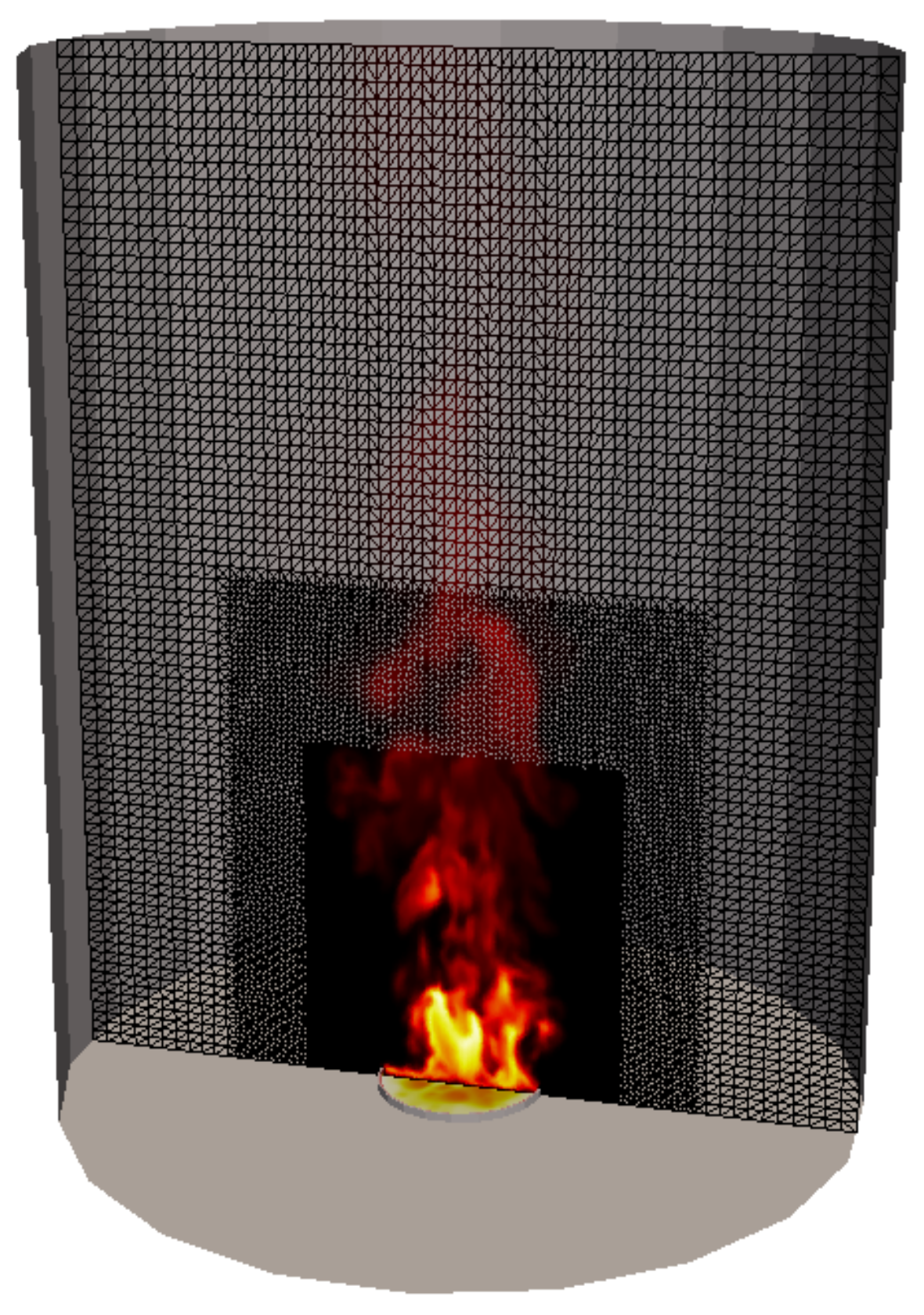
The target test case includes the medium-scale (i.e., 30 cm) methanol pool fire (i.e., 19 kW) experiments reported by Kim et al. [60] while the presented numerical results are reproduced from [67]. A cylindrical domain having dimensions 1.5 m × 1.8 m was used to model the case. The base mesh consisted of 2 cm cells on the centreline which were then stretched towards the side and top boundaries of the domain (i.e., ratio of initial to final grid size was 1.5). A local grid refinement strategy was then employed in order to have a grid resolution of 0.5 cm in the near-field region of the pool fires (i.e., see Figure 3). Turbulence was modelled with the dynamic Smagorinsky model employing a variable Prandtl number approach. Chemistry was considered to be infinitely fast and turbulence-chemistry interactions were modelled with the Eddy Dissipation Model (EDM) considering a turbulent mixing time scale (i.e., $C_{EDM}=2$). Radiation was modelled with the finite volume discrete ordinates model (fvDOM) and the absorption/emission term was modelled through the weighted sum of gray gases model (WSGGM). In total, 72 solid angles were used for angular discretization in the solution of the radiative transfer equation (i.e., with radiation solved every 20th time step). The characteristic lengths, $L_c$, for the natural and forced convection modelling approaches presented below are chosen as $L_{c, natural}=A_s/p=0.075$ m and $L_{c, forced}=D=0.3$ m, respectively (see Section 3.1.3).

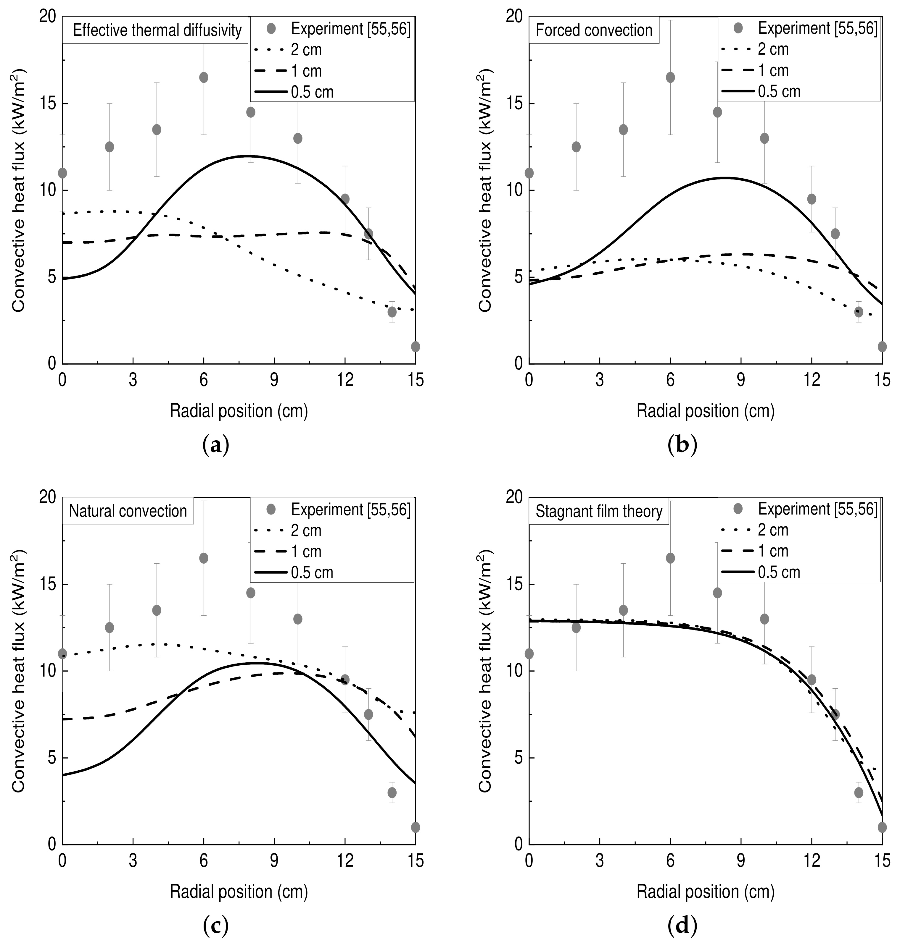
The predicted convective heat fluxes at the methanol pool surface with different approaches for modelling the convection are presented in Figure 4. Overall, a strong grid dependency is observed in the predictions with the approaches based on the effective thermal diffusivity, forced and natural convection (i.e., for all methods directly relying on the first grid cell values when determining the convective heat fluxes). With the use of coarse grid sizes (i.e., few cells across the pool diameter), fuel and oxidiser mix rapidly and produce high reaction rates above the pool surface. As the grid size is refined (i.e., more cells across the pool diameter), a fuel-rich region starts to develop, which then produces lower reaction rates above the pool surface. The result of this is that higher temperature differences (i.e., calculated based on the first grid cell and the surface temperature) are obtained when coarser cells are used as opposed to finer cells. This resulting decrease in the temperature difference, $\Delta T$, when the grid becomes smaller affects the calculated convective heat fluxes directly (i.e., through Newton’s law) as well as the calculated Grashof numbers for natural convection scenarios indirectly. The forced convection approach is not significantly affected by this aspect as it does not directly depend on temperature, rather on the velocity in the first grid cell which remains fairly constant around the centreline. Nevertheless, a noticeable grid dependency is observed at radial locations which are off-centre. The approach based on the stagnant film theory (i.e., Equation (40)), for which the convective heat fluxes do not directly depend on the local gas phase temperature (i.e., rather temperature is only used for the calculation of the convective heat transfer coefficient h), shows minimal effects of grid dependency. The reader is referred to [24,25], where additional analysis is included as well as the predicted temperature and velocity fields above the surface of the methanol pool fires are presented.

5.2. Flame Spread

The target test case includes the Single Burning Item (SBI) experiments with Medium Density Fiberboard (MDF) reported by Zeinali et al. [74,75]. The experiments include two flammable walls (i.e., long and short) positioned perpendicular to each other to form a corner (see Figure 5). The widths of the long and short walls are 1 m and 0.5 m, respectively, while their height is 1.5 m. A 30 kW triangular propane (C${}_3$H${}_8$) burner is used as fire source having a side dimension of 0.25 m, located at the corner at a distance of 0.04 m from the walls. There is a ramp-up time of 30 s until the peak HRR of the burner is reached. The presented numerical results are reproduced from [12]. The computational domain has a rectangular shape with dimensions of 1 m × 2 m × 1 m (length × height × width). A local grid refinement was considered using mesh sizes ranging between 1 cm to 4 cm, focusing on having the smaller grid resolution in locations where burning would occur (see Figure 5). The dynamic Smagorinsky model was used to model turbulence together with a dynamic procedure for the Prandtl number. Chemistry was considered to be infinitely fast and the Eddy Dissipation Model (EDM) (i.e., $C_{EDM}=2$) was used for modelling the turbulence–chemistry interactions. The finite volume discrete ordinates model (fvDOM) was used for radiation, neglecting absorption and modelling the emission term through the constant radiative fraction approach. The global radiative fraction, ${\chi }_r$, in the simulations varied between ${\chi }_{r, burner}=0.25$ and ${\chi }_{r, wall}=0.35$ depending on the mass flow rates of burner and the burning walls. In total, 72 solid angles were used for angular discretization in the solution of the radiative transfer equation (i.e., with radiation solved every 20th time step). For the thermal decomposition of the solid walls a simplified 1D pyrolysis model was employed which solved conservation equations for mass and energy using a fully implicit scheme. Pyrolysis was modelled using a single-step Arrhenius reaction considering three species: virgin material, char and pyrolysate. More details regarding the modelling as well as the optimised material used for the MDF walls are provided in [12]. The characteristic lengths, $L_c$, for the natural convection modelling approach presented below is chosen as $L_{c, natural}=1.5$ m (i.e., height of walls—see Section 3.1.3).

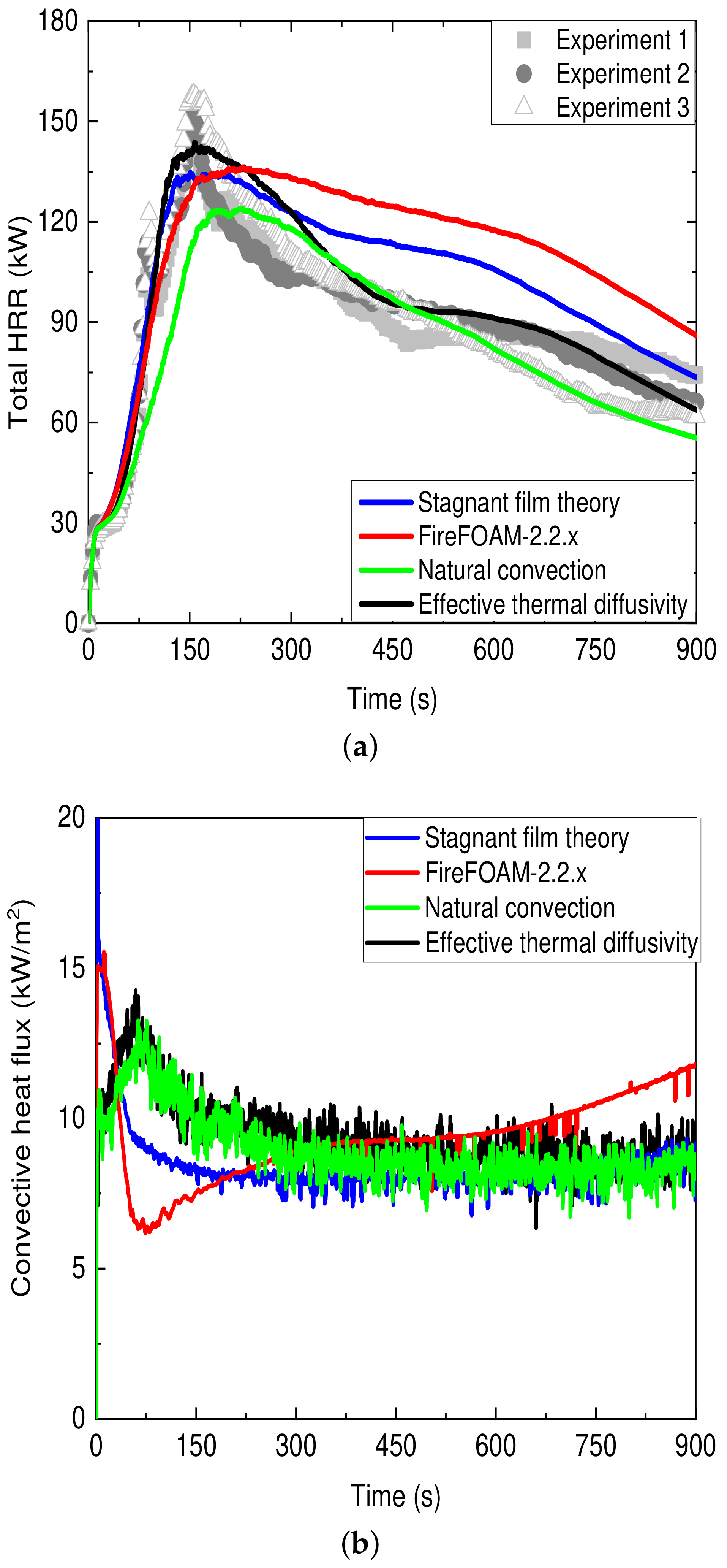
The evolution of the total (i.e., burner plus walls) heat release rate and the convective heat fluxes at sensor S1 (i.e., located on the long wall and positioned 21 cm from the bottom and 5 cm from the corner) as a function of time, with different approaches for modelling convective heat transfer, is presented in Figure 6. Given the uncertainties related to gas phase (i.e., turbulence, combustion, radiation and heat transfer) and solid phase (i.e., pyrolysis) modelling, the predictions using the effective thermal diffusivity are fairly good when compared to the experiments. More specifically, the predicted initial flame growth period, the maximum value of the HRR as well as the burning of the walls during the decay phase are all fairly well predicted. The predictions of the stagnant film theory approach were fair in the initial flame growth period but under-estimated the maximum value of the HRR and over-estimated the burning intensity of the flammable walls in the decay phase. These discrepancies can be potentially linked to the calculation of the convection coefficient which does not consider the local flow properties. The approach based on natural convection predicted well the decay phase but under-estimated both the maximum HRR value and the initial flame growth period, with the discrepancies possible stemming from the temperature sensitivity in the calculation of the convection coefficient. Nevertheless, it is worth noting that the blowing effect is neglected with this approach, which would essentially further reduce the predicted convective heat fluxes and would result in lower HRR predictions. Finally, the approach employed in FireFOAM 2.2.x predicted with fair accuracy the initial flame growth period but under-estimated the maximum value of the HRR and performed poorly in the decay phase by over-estimating the burning of the walls. A possible reason for the discrepancies could be that the convective heat fluxes are not calculated considering the local flow properties, rather only change in the presence of mass transfer [12].

Overall, convective heat transfer can be potentially be important in upward flame spread scenarios. Convective heat transfer contributes to the pre-heating of the virgin material during the early stages of flame spread and failing to accurately model it can greatly affect the burning behaviour (i.e., time to reach the maximum HRR, the maximum HRR value, decay phase) of flammable surfaces.

6. Concluding Remarks

The present paper focused on convective heat transfer and presented a review of the most commonly used approaches for modelling convective heat transfer with CFD, using Large Eddy Simulations (LES), in the context of fire-driven flows. The main assumptions, advantages and disadvantages of each modelling approach were outlined. The target cases that were examined mainly involved pool fires and turbulent wall fires, geometries that are very common and of practical importance in most fire scenarios. Numerical results from the application of different approaches for modelling convection were also presented in order to illustrate the influence that convective heat transfer can have in scenarios where the heat feedback to the fuel surface can be important (e.g., flame spread cases).

In general, more experimental data for individual heat flux components (i.e., radiative and convective) are needed for medium and large-scale flame spread scenarios. Currently, this is not the case due to experimental uncertainties/limitations. Nevertheless, measurements of local heat fluxes in simpler scenarios, e.g., involving steady laminar boundary layer diffusion flames [13], do exist in literature even though such conditions are not representative of typical fire cases. Often, model ‘validation’ is performed by considering (convective/radiative) heat fluxes obtained from fine-grained simulations (see e.g., [11,51,54,55]) which even though can be a good alternative it is also not necessarily free of errors (e.g., due to combustion/radiation modelling uncertainties in the region near the wall and challenging low dissipative schemes). Similar difficulties are also present in the context of pool fires and pose limitations for the validation of convective heat transfer models. Experimental measurements typically report the total heat fluxes and estimation of the convective component is made through the use of the stagnant film theory, e.g., [60,76]. The development of an experimental database, reporting on accurate measurements of convective heat fluxes for a range of fire scenarios, would be helpful towards further improving the accuracy of convection modelling with CFD codes.

References

- Drysdale, D. An Introduction to Fire Dynamics; Wiley & Sons: Hoboken, NJ, USA, 2011. [Google Scholar]
- Tieszen, S.R. On the fluid mechanics of fires. Annu. Rev. Fluid Mech. 2001, 33, 67–92. [Google Scholar] [CrossRef] [Green Version]
- Joulain, P. Convective and radiative transport in pool and wall fires: 20 years of research in Poitiers. Fire Saf. J. 1996, 26, 99–149. [Google Scholar] [CrossRef]
- Joulain, P. The behavior of pool fires: State of the art and new insights. Proc. Comb. Inst. 1998, 27, 2691–2706. [Google Scholar] [CrossRef]
- Piomelli, U.; Balaras, E. Wall-layer models for large-eddy simulations. Annu. Rev. Fluid Mech. 2002, 34, 349–374. [Google Scholar] [CrossRef] [Green Version]
- Brown, A.; Bruns, M.; Gollner, M.; Hewson, J.; Maragkos, G.; Marshall, A.; McDermott, R.; Merci, B.; Rogaume, T.; Stoliarov, S.; et al. Proceedings of the first workshop organized by the IAFSS Working Group on Measurement and Computation of Fire Phenomena (MaCFP). Fire Saf. J. 2018, 101, 1–17. [Google Scholar] [CrossRef]
- Hamins, A.; Fischer, S.J.; Kashiwagi, T.; Klassen, M.E.; Gore, J.P. Heat Feedback to the Fuel Surface in Pool Fires. Combust. Sci. Technol. 1994, 97, 37–62. [Google Scholar] [CrossRef]
- Steinhaus, T.; Welch, S.; Carvel, R.O.; Torero, J.L. Large-scale pool fires. Therm. Sci. 2007, 11, 101–118. [Google Scholar] [CrossRef]
- Quintiere, J.G. Fundamentals of Fire Phenomena; Wiley & Sons: Hoboken, NJ, USA, 2006. [Google Scholar]
- Hu, L. A review of physics and correlations of pool fire behaviour in wind and future challenges. Fire Saf. J. 2017, 91, 41–55. [Google Scholar] [CrossRef]
- Ren, N.; Wang, Y. A Convective Heat Transfer Model for LES Fire Modeling. Proc. Comb. Inst. 2021, 38, 4535–4542. [Google Scholar] [CrossRef]
- Maragkos, G.; Zeinali, D.; Merci, B. Influence of convective heat transfer modelling in CFD simulations of upward flame spread. Fire Saf. J. 2021, 122, 103347. [Google Scholar] [CrossRef]
- Singh, A.V.; Gollner, M.J. A methodology for estimation of local heat fluxes in steady laminar boundary layer diffusion flames. Combust. Flame 2015, 162, 2214–2230. [Google Scholar] [CrossRef]
- Incropera, F.P.; DeWitt, D.P.; Bergman, T.L.; Lavine, A.S. Fundamentals of Heat and Mass Transfer, 6th ed.; John Wiley & Sons: New York, NY, USA, 2006. [Google Scholar]
- Orloff, L.; de Ris, J. Froude Modeling of Pool Fires; Technical Report No. RC81-BT-9; Factory Mutual Research: Norwood, MA, USA, 1982. [Google Scholar]
- Orloff, L.; de Ris, J. Froude Modeling of Pool Fires. Symp. Combust. 1982, 19, 885–895. [Google Scholar] [CrossRef]
- Mitler, H.E. Algorithm for the Mass-loss Rate of A Burning Wall. Fire Saf. Sci. 1989, 2, 179–188. [Google Scholar] [CrossRef] [Green Version]
- Tewarson, A. Smoke Point Height and Fire Properties of Materials; NIST-GCR-88-555; National Institute of Standards and Technology: Gaithersburg, MD, USA, 1988.
- Quintiere, J.G. A Semi-Quantitative Model for the Burning Rate of Solid Materials. Fire Saf. Sci. 1992, 1, 3–25. [Google Scholar]
- Orloff, L.; de Ris, J.; Markstein, G.H. Upward turbulent fire spread and burning of fuel surface. Symp. Combust. 1975, 15, 183–192. [Google Scholar] [CrossRef]
- Orloff, L.; Modak, A.T.; Alpert, R.L. Burning of large-scale vertical surfaces. Symp. Combust. 1977, 16, 1345–1354. [Google Scholar] [CrossRef]
- FireFOAM Code Website. Available online: https://github.com/fireFoam-dev (accessed on 14 March 2021).
- Fire Dynamics Simulator (FDS) Code. Available online: https://pages.nist.gov/fds-smv/ (accessed on 14 March 2021).
- Maragkos, G.; Beji, T.; Merci, B. Advances in modelling in CFD simulations of turbulent gaseous pool fires. Combust. Flame 2017, 181, 22–38. [Google Scholar] [CrossRef]
- Maragkos, G.; Beji, T.; Merci, B. Towards predictive simulations of gaseous pool fires. Proc. Comb. Inst. 2019, 37, 3927–3934. [Google Scholar] [CrossRef]
- Maragkos, G.; Merci, B. On the use of dynamic turbulence modelling in fire applications. Combust. Flame 2020, 26, 9–23. [Google Scholar] [CrossRef]
- Smagorinsky, J. General Circulation Experiments with the Primitive Equations. I. The Basic Experiment. Mon. Weather Rev. 1963, 91, 99–164. [Google Scholar] [CrossRef]
- Moin, P.; Squires, K.; Cabot, W.H.; Lee, S. A dynamic subgrid-scale model for compressible turbulence and scalar transport. Phys. Fluids A 1991, 3, 2746–2757. [Google Scholar] [CrossRef]
- Deardorff, J.W. Stratocumulus-capped mixed layers derived from a three-dimensional model. Bound. Layer Meteorol. 1980, 18, 495–527. [Google Scholar] [CrossRef]
- Magnussen, B.F.; Hjertager, B.H. On mathematical modeling of turbulent combustion with special emphasis on soot formation and combustion. Proc. Comb. Inst. 1977, 16, 719–729. [Google Scholar] [CrossRef]
- Modest, M.F. The Weighted-Sum-of-Gray-Gases Model for Arbitrary Solution Methods in Radiative Transfer. J. Heat Transf. 1991, 113, 650–656. [Google Scholar] [CrossRef]
- McAdams, W.H. Heat Transmission; McGraw-Hill Book Company: New York, NY, USA, 1957. [Google Scholar]
- Welty, J.; Rorrer, G.L.; Foster, D.G. Fundamentals of Momentum, Heat and Mass Transfer; John Wiley & Sons: New York, NY, USA, 2014. [Google Scholar]
- Holman, J.P. Heat Transfer, 10th ed.; McGraw-Hill: New York, NY, USA, 2010. [Google Scholar]
- Ranz, W.E.; Marshall, W.R. Evaporation from Drops. Chem. Eng. Prog. 1952, 48, 141–146. [Google Scholar]
- Churchill, S.W.; Chu, H.H.S. Correlating Equations for Laminar and Turbulent Free Convection from a Vertical Plate. Int. J. Heat Mass Transf. 1975, 18, 1323–1329. [Google Scholar] [CrossRef]
- Churchill, S.W. Free Convection around Immersed Bodies. In Heat Exchanger Design Handbook; Hemisphere Publishing: New York, NY, USA, 1983. [Google Scholar]
- Chen, Q.; Zhai, Z. The use of CFD tools for indoor environmental design. In Advanced Building Simulation; Spon Press: New York, NY, USA, 2004; pp. 119–140. [Google Scholar]
- Petrik, M.; Erdos, A.; Jarmai, K.; Szepesi, G. Optimum design of an air tank for fatigue and fire load. Acta Polytech. Hung. 2021, 18, 163–177. [Google Scholar] [CrossRef]
- Zhai, Z.; Chen, Q.Y. Numerical determination and treatment of convective heat transfer coefficient in the coupled building energy and CFD simulation. Build. Environ. 2004, 39, 1001–1009. [Google Scholar] [CrossRef]
- Beji, T.; Merci, B. Development of a numerical model for liquid pool evaporation. Fire Saf. J. 2018, 102, 48–58. [Google Scholar] [CrossRef]
- Hamins, A.P.; Yang, J.C.; Kashiwagi, T. Global Model for Predicting the Burning Rates of Liquid Pool Fires; NIST Interagency/Internal Report (NISTIR)-6381; National Institute of Standards and Technology: Gaithersburg, MD, USA, 1999.
- Sikanen, T.; Hostikka, S. Modelling and simulation of liquid pool fires with in-depth and heat transfer. Fire Saf. J. 2016, 80, 95–109. [Google Scholar] [CrossRef]
- Markus, E.; Snegirev, A.; Kuznetsov, E.; Tanklevskiy, L. Application of the thermal pyrolysis model to predict flame spread over continuous and discrete fire load. Fire Saf. J. 2019, 108, 102825. [Google Scholar] [CrossRef]
- Launder, B.E.; Spalding, D.B. The Numerical Computation of Turbulent Flows. Comput. Methods Appl. Mech. Eng. 1974, 3, 269–289. [Google Scholar] [CrossRef]
- McGrattan, K.; Hostikka, S.; Floyd, J.; McDermott, R.; Vanella, M. Fire Dynamics Simulator Technical Reference Guide Volume 1: Mathematical Model, 6th ed.; NIST Special Publication 1018-1; National Institute of Standards and Technology: Gaithersburg, MD, USA, 2020.
- Pope, S.B. Turbulent Flows; Cambridge University Press: Cambridge, UK, 2000. [Google Scholar]
- Werner, H.; Wengle, H. Large-eddy simulation of turbulent flow over and around a cube in a plate channel. In Proceedings of the 8th Symposium on Turbulent Shear Flows, Munich, Germany, 9–11 September 1991; pp. 155–168. [Google Scholar]
- Kader, B.A. Temperature and concentration profiles in fully turbulent boundary layers. Int. J. Heat Mass Transf. 1981, 24, 1541–1544. [Google Scholar] [CrossRef]
- Yan, Z.; Holmstedt, G. CFD Simulation of Upward Flame Spread over Fuel Surface. Fire Saf. Sci. 1997, 5, 345–356. [Google Scholar] [CrossRef] [Green Version]
- Ren, N.; Wang, Y.; Vilfayeau, S.; Trouvé, A. Large Eddy Simulation of Propylene Turbulent Vertical Wall Fires. In Proceedings of the Seventh International Seminar on Fire and Explosion Hazards, Providence, RI, USA, 5–10 May 2013. [Google Scholar]
- Ren, N.; Wang, Y.; Trouvé, A. Large Eddy Simulation of Vertical Turbulent Wall Fires. Procedia Eng. 2013, 33, 443–452. [Google Scholar] [CrossRef] [Green Version]
- Fukumoto, K.; Wang, C.; Wen, J. Large eddy simulation of upward flame spread on PMMA walls with a fully coupled fluid–solid approach. Combust. Flame 2018, 190, 365–387. [Google Scholar] [CrossRef] [Green Version]
- Ren, N.; Wang, Y.; Vilfayeau, S.; Trouvé, A. Large eddy simulation of turbulent vertical wall fires supplied with gaseous fuel through porous burners. Combust. Flame 2016, 169, 194–208. [Google Scholar] [CrossRef]
- Li, K.; Hostikka, S. Embedded flame heat flux method for simulation of quasi-steady state vertical flame spread. Fire Saf. J. 2019, 104, 117–129. [Google Scholar] [CrossRef] [Green Version]
- McDermott, R.J. Quality assessment in the fire dynamics simulator: A bridge to reliable simulations. In Proceedings of the Fire and Evacuation Modeling Technical Conference, Baltimore, MD, USA, 15–16 August 2011. [Google Scholar]
- Ahmad, T.; Faeth, G.M. Turbulent wall fires. Proc. Comb. Inst. 1979, 17, 1149–1160. [Google Scholar] [CrossRef]
- Glassman, I. Combustion; Academic Press: New York, NY, USA, 1977. [Google Scholar]
- Klassen, M.; Gore, J.P. Structure and Radiation Properties of Pool Fires; NIST GCR 94-651; National Institute of Standards and Technology: Gaithersburg, MD, USA, 1994.
- Kim, S.C.; Lee, K.Y.; Hamins, A. Energy Balance in Medium-Scale Methanol, Ethanol, and Acetone Pool Fires. Fire Saf. Sci. 2019, 107, 44–53. [Google Scholar]
- Zeinali, D.; Gupta, A.; Maragkos, G.; Agarwal, G.; Beji, T.; Chaos, M.; Wang, Y.; Degroote, J.; Merci, B. Study of the importance of non-uniform mass density in numerical simulations of fire spread over MDF panels in a corner configuration. Combust. Flame 2019, 200, 303–315. [Google Scholar] [CrossRef] [Green Version]
- Wang, Y.; Meredith, K.V.; Zhou, X.; Chatterjee, P.; Xin, Y.; Chaos, M.; Ren, N.; Dorofeev, S.B. Numerical Simulation of Sprinkler Suppression of Rack Storage Fires. Fire Saf. Sci. 2014, 11, 1170–1183. [Google Scholar] [CrossRef]
- Ren, N.; de Vries, J.; Zhou, X.; Chaos, M.; Meredith, K.V.; Wang, Y. Large-scale fire suppression modeling of corrugated cardboard boxes on wood pallets in rack-storage configurations. Fire Saf. J. 2017, 91, 695–704. [Google Scholar] [CrossRef]
- Hamins, A. Energetics of Small and Moderate-Scale Gaseous Pool Fires; NIST Technical Note 1926; National Institute of Standards and Technology: Gaithersburg, MD, USA, 2016.
- Nasr, A.; Suard, S.; El-Rabii, H.; Gay, J.; Garo, J.-P. Fuel Mass-Loss Rate Determination in a Confined and Mechanically Ventilated Compartment Fire Using a Global Approach. Combust Sci. Technol. 2011, 183, 1342–1359. [Google Scholar] [CrossRef]
- Suard, S.; Nasr, A.; Melis, S.; Garo, J.P.; El-Rabii, H.; Gay, L.; Rigollet, L.; Audouin, L. Analytical Approach for Predicting Effects of Vitiated Air on the Mass Loss Rate of Large Pool Fire in Confined Compartments. Fire Saf. Sci. 2011, 10, 1513–1524. [Google Scholar] [CrossRef]
- Maragkos, G.; Merci, B. Grid insensitive modelling of convective heat transfer fluxes in CFD simulations of medium-scale pool fires. Fire Saf. J. 2020, 120, 103104. [Google Scholar] [CrossRef]
- Ritchie, S.J.; Steckler, K.D.; Hamins, A.; Cleary, T.G.; Yang, J.C.; Kashiwagi, T. The Effect of Sample Size on the Heat Release Rate of Charring Materials. Fire Saf. Sci. 1997, 5, 177–188. [Google Scholar] [CrossRef]
- Fukumoto, K.; Wen, J.X.; Li, M.; Yanming, D.; Changjian, W. Numerical simulation of small pool fires incorporating liquid fuel motion. Combust. Flame 2020, 213, 441–454. [Google Scholar] [CrossRef]
- Xu, B.; Wen, J. The effect of convective motion within liquid fuel on the mass burning rates of pool fires—A numerical study. Proc. Comb. Inst. 2021, 38, 4979–4986. [Google Scholar] [CrossRef]
- Vali, A.; Nobes, D.S.; Kostiuk, L.W. Fluid motion and energy transfer within burning liquid fuel pools of various thicknesses. Combust. Flame 2015, 162, 1447–1488. [Google Scholar] [CrossRef]
- Beji, T. Theoretical analysis of the liquid thermal structure in a pool fire. J. Fire Sci. 2021, 39, 36–52. [Google Scholar] [CrossRef]
- Ahmed, M.M.; Trouvé, A. Large eddy simulation of the unstable flame structure and gas-to-liquid thermal feedback in a medium-scale methanol pool fire. Combust. Flame 2021, 225, 237–254. [Google Scholar] [CrossRef]
- Zeinali, D.; Verstockt, S.; Beji, T.; Maragkos, G.; Degroote, J.; Merci, B. Experimental study of corner fires: Part II: Flame spread over MDF panels. Combust. Flame 2018, 189, 491–505. [Google Scholar] [CrossRef]
- Zeinali, D. Flame Spread and Fire Behavior in a Corner Configuration. Ph.D. Thesis, Ghent University, Ghent, Belgium, 2019. [Google Scholar]
- Sung, K.; Chen, J.; Bundy, M.; Hamins, A. The characteristics of a 1 m methanol pool fire. Fire Saf. Sci. 2021, 120, 103121. [Google Scholar] [CrossRef]
Figure 1.
Characteristic length, , for (a) forced and (b) natural convection scenarios. and p are the surface area and perimeter of the plate, respectively.
Figure 2.
Magnitude of the (Equation (39)) factor for several fuels and pool diameters. Experimental data for the mass loss rate per unit area taken from [59,60].
Figure 3.
Overview of the computational domain, local grid refinement (i.e., 2 cm, 1 cm, 0.5 cm) employed in the numerical simulation of the 30 cm methanol pool fire [67].
Figure 4.
Average convective heat fluxes at the methanol pool surface as a function of grid size with the approach based on (a) the effective thermal diffusivity, (b) forced convection, (c) natural convection and (d) the stagnant film theory. Experimental data from [59,60] and simulation results from Maragkos et al. [67].
Figure 5.
Illustration of the computational mesh used in the numerical simulations. Figure reproduced from [12].
Figure 6.
Temporal evolution of the (a) total (i.e., burner plus walls) heat release rate and (b) the convective heat fluxes at sensor S1 with different approaches for modelling convection. Experimental data from Zeinali et al. [74,75] and simulation results from Maragkos et al. [12].