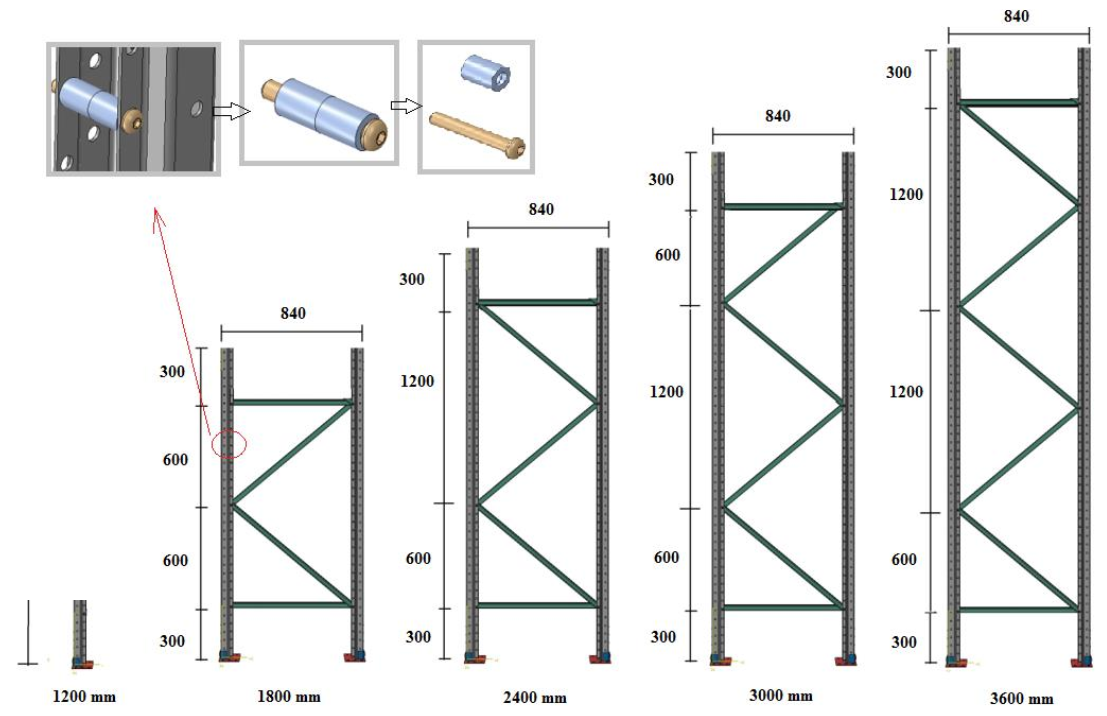
Figure 1.
Schematic of models.
Figure 1.
Schematic of models.
Figure 2.
Coupon test results for uprights: (
a) with 1.6 mm, and (
b) with 2.5 mm thickness [
9].
Figure 2.
Coupon test results for uprights: (
a) with 1.6 mm, and (
b) with 2.5 mm thickness [
9].
Figure 3.
Interactions between frame elements.
Figure 3.
Interactions between frame elements.
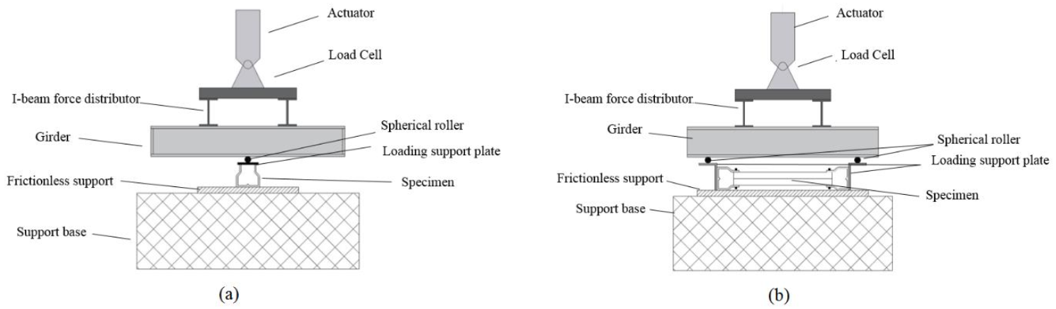
Figure 4.
(
a) Minor axis test setup. (
b) Major axis test setup [
9].
Figure 4.
(
a) Minor axis test setup. (
b) Major axis test setup [
9].
Figure 5.
Typical FE mesh of an upright section.
Figure 5.
Typical FE mesh of an upright section.
Figure 6.
Comparison of the FE model against the minor-axis test results for (a) non-reinforced model, (b) 200 mm reinforced model and (c) 300 mm reinforced model.
Figure 6.
Comparison of the FE model against the minor-axis test results for (a) non-reinforced model, (b) 200 mm reinforced model and (c) 300 mm reinforced model.
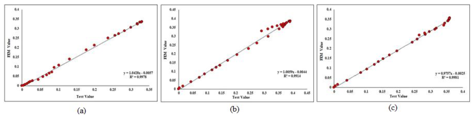
Figure 7.
Linear regression diagram for (a) non-reinforced model, (b) 200 mm reinforced model, and (c) 300 mm reinforced model.
Figure 7.
Linear regression diagram for (a) non-reinforced model, (b) 200 mm reinforced model, and (c) 300 mm reinforced model.
Figure 8.
Comparison of FE model against major-axis test results for (a) non-reinforced model, (b) 200 mm reinforced model and (c) 300 mm reinforced model.
Figure 8.
Comparison of FE model against major-axis test results for (a) non-reinforced model, (b) 200 mm reinforced model and (c) 300 mm reinforced model.
Figure 9.
Linear regression diagram for; (a) non-reinforced model, (b) 200 mm reinforced model, and (c) 300 mm reinforced model.
Figure 9.
Linear regression diagram for; (a) non-reinforced model, (b) 200 mm reinforced model, and (c) 300 mm reinforced model.
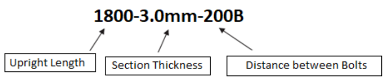
Figure 10.
Designation of models.
Figure 10.
Designation of models.
Figure 11.
Normalized moment-deflection curves for 1800 mm models about major axis.
Figure 11.
Normalized moment-deflection curves for 1800 mm models about major axis.
Figure 12.
Normalized moment-deflection curves for 2400 mm models about major axis.
Figure 12.
Normalized moment-deflection curves for 2400 mm models about major axis.
Figure 13.
Normalized moment-deflection curves for 3000 mm models about major axis.
Figure 13.
Normalized moment-deflection curves for 3000 mm models about major axis.
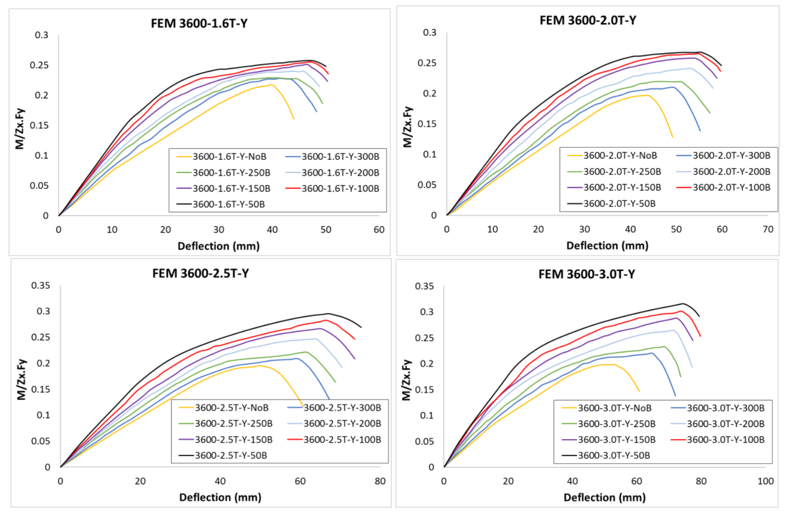
Figure 14.
Normalized moment-deflection curves for 3600 mm models about major axis.
Figure 14.
Normalized moment-deflection curves for 3600 mm models about major axis.
Figure 15.
The normalized ultimate moment of 1800, 2400, 3000, and 3600 mm models about major axis with respect to reinforcement spacing.
Figure 15.
The normalized ultimate moment of 1800, 2400, 3000, and 3600 mm models about major axis with respect to reinforcement spacing.
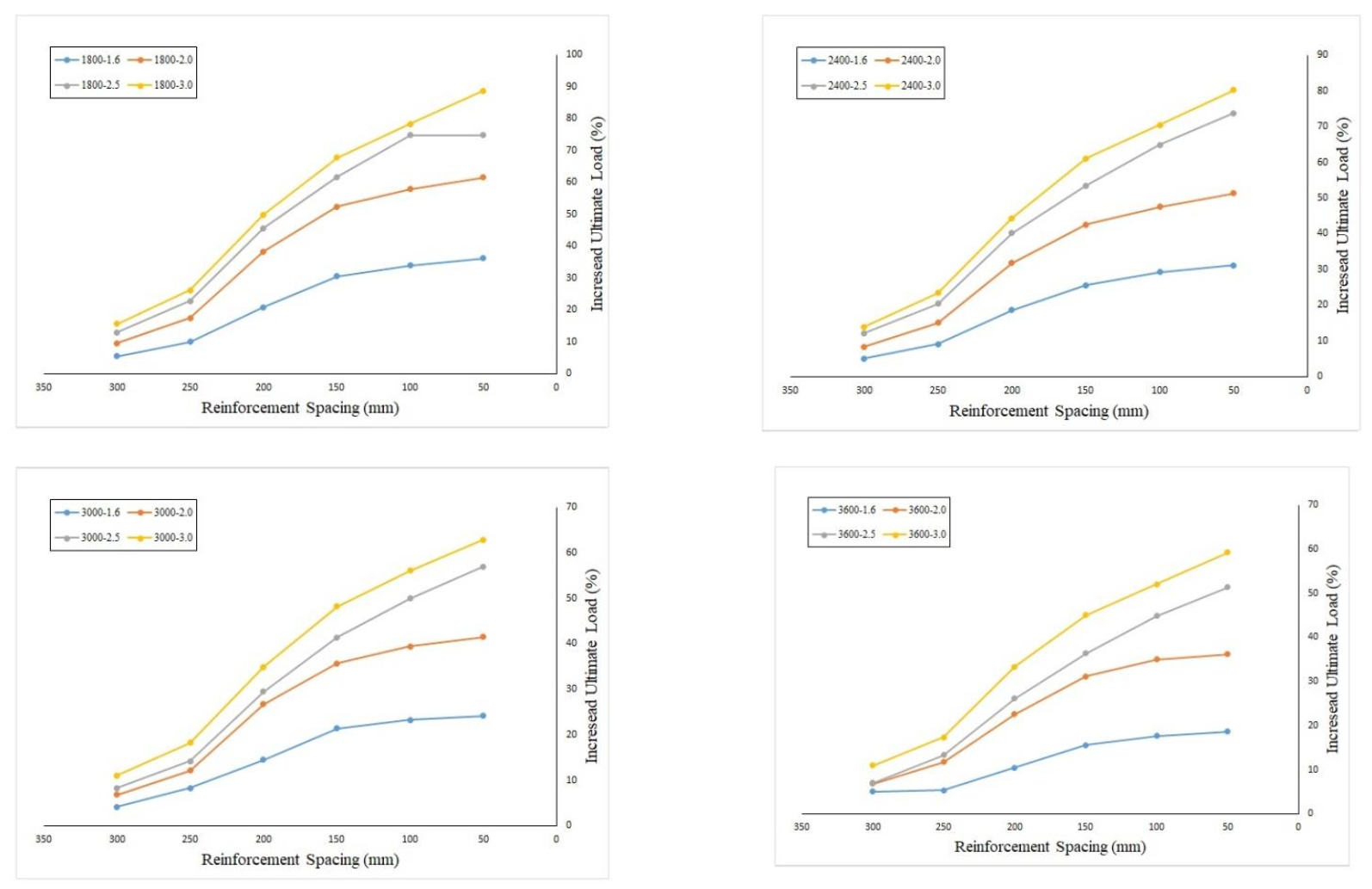
Figure 16.
Percentage of increased ultimate load of major axis analysis with different reinforcement spacing in length order.
Figure 16.
Percentage of increased ultimate load of major axis analysis with different reinforcement spacing in length order.
Figure 17.
Normalized moment-deflection curves for 1800 mm models about minor axis.
Figure 17.
Normalized moment-deflection curves for 1800 mm models about minor axis.
Figure 18.
Normalized moment-deflection curves for 2400 mm models about minor axis.
Figure 18.
Normalized moment-deflection curves for 2400 mm models about minor axis.
Figure 19.
Normalized moment-deflection curves for 3000 mm models about minor axis.
Figure 19.
Normalized moment-deflection curves for 3000 mm models about minor axis.
Figure 20.
Normalized moment-deflection curves for 3600 mm models about minor axis.
Figure 20.
Normalized moment-deflection curves for 3600 mm models about minor axis.
Figure 21.
The normalized ultimate moment of 1800, 2400, 3000, 3600 mm models about minor axis with respect to reinforcement spacing.
Figure 21.
The normalized ultimate moment of 1800, 2400, 3000, 3600 mm models about minor axis with respect to reinforcement spacing.
Figure 22.
Percentage of increased ultimate load with different reinforcement.
Figure 22.
Percentage of increased ultimate load with different reinforcement.
Figure 23.
Schematic representation of MLP neuron.
Figure 23.
Schematic representation of MLP neuron.
Figure 24.
Visualization of a single hidden layer MLP network.
Figure 24.
Visualization of a single hidden layer MLP network.
Figure 25.
PSO sequential flowchart.
Figure 25.
PSO sequential flowchart.
Figure 26.
Feature selection technique steps.
Figure 26.
Feature selection technique steps.
Figure 27.
Flowchart of the sequential combination of hybrid MLP–PSO–FS algorithm.
Figure 27.
Flowchart of the sequential combination of hybrid MLP–PSO–FS algorithm.
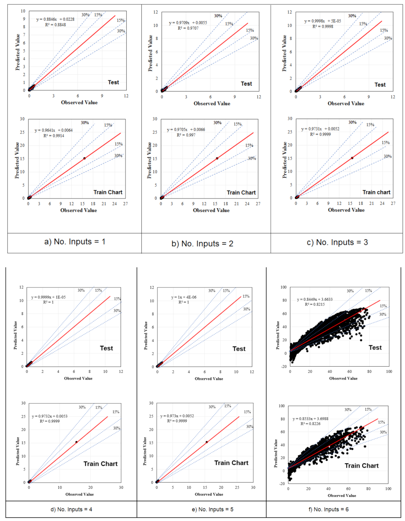
Figure 28.
Comparison of the predicted and measured load: (a) One input, (b) two inputs, (c) three inputs, (d) four input, (e) five inputs, (f) six inputs through MLP–PSO–FS model.
Figure 28.
Comparison of the predicted and measured load: (a) One input, (b) two inputs, (c) three inputs, (d) four input, (e) five inputs, (f) six inputs through MLP–PSO–FS model.
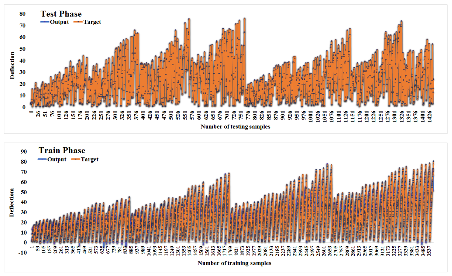
Figure 29.
MLP–PSO–FS (4 inputs) prediction vs. experimental diagram: (above) train phase, (below) test phase.
Figure 29.
MLP–PSO–FS (4 inputs) prediction vs. experimental diagram: (above) train phase, (below) test phase.
Figure 30.
MLP–PSO–FS (4 inputs) Error histograms: (above) train phase, (below) test phase.
Figure 30.
MLP–PSO–FS (4 inputs) Error histograms: (above) train phase, (below) test phase.
Figure 31.
MLP–PSO–FS regression charts (iteration = 100): (a) P150, (b) P250, (c) P350.
Figure 31.
MLP–PSO–FS regression charts (iteration = 100): (a) P150, (b) P250, (c) P350.
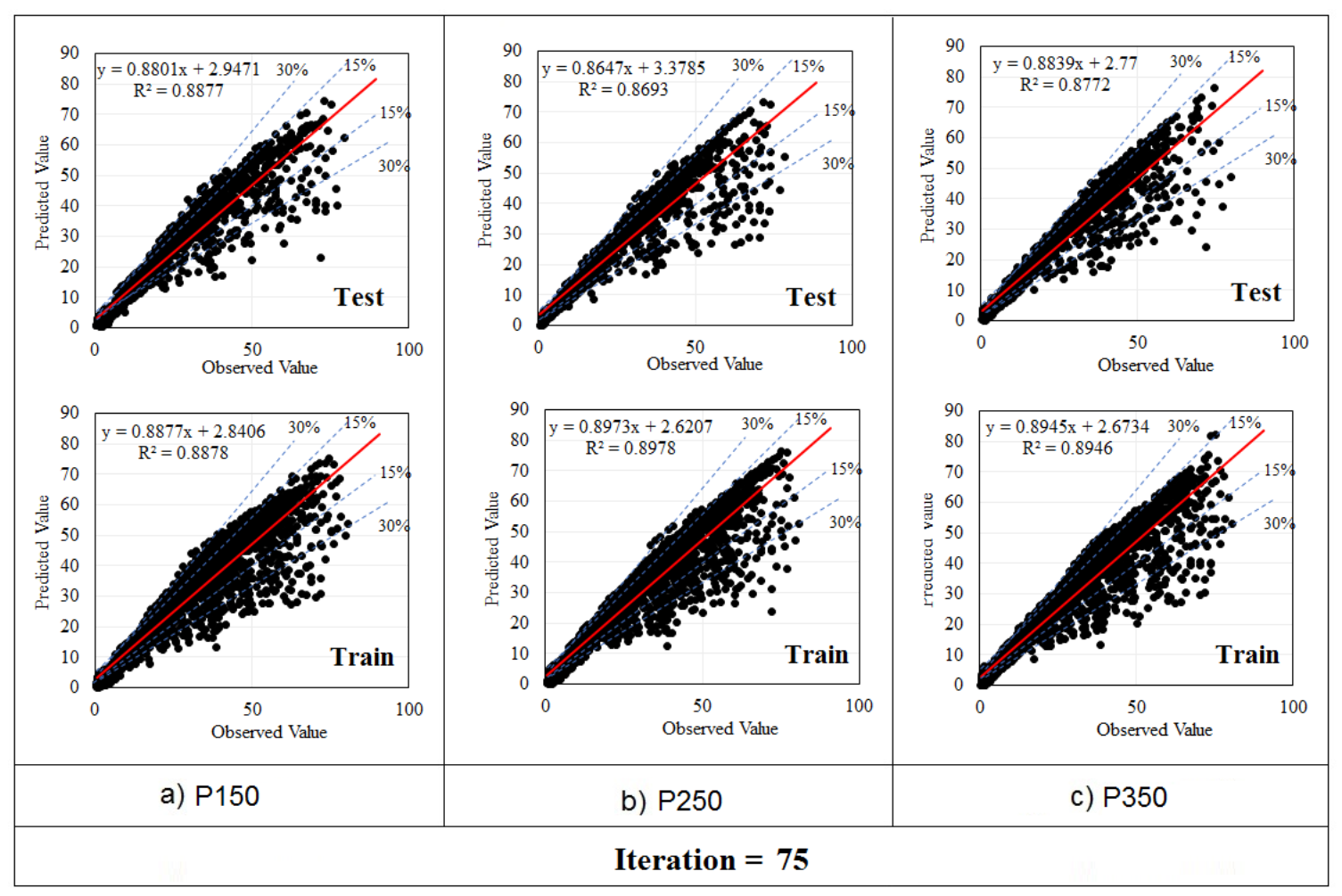
Figure 32.
MLP–PSO–FS regression charts (iteration = 75): (a) P150, (b) P250, (c) P350.
Figure 32.
MLP–PSO–FS regression charts (iteration = 75): (a) P150, (b) P250, (c) P350.
Figure 33.
MLP–PSO–FS regression charts (iteration = 45): (a) P150, (b) P250, (c) P350.
Figure 33.
MLP–PSO–FS regression charts (iteration = 45): (a) P150, (b) P250, (c) P350.
Figure 34.
MLP–PSO–FS (6 inputs) prediction vs. experimental diagram: (above) train phase, (below) test phase.
Figure 34.
MLP–PSO–FS (6 inputs) prediction vs. experimental diagram: (above) train phase, (below) test phase.
Figure 35.
PSO–FS (6 inputs) error histograms: (above) train phase, (below) test phase.
Figure 35.
PSO–FS (6 inputs) error histograms: (above) train phase, (below) test phase.
Table 1.
Geometrical features of models.
Table 1.
Geometrical features of models.
| Upright Length (mm) | Upright Thickness (mm) | Reinforcement Spacing (mm) |
|---|
| 1800 | 1.6
2.0
2.5
3.0 | 50
100
150
200
250
300 |
| 2400 |
| 3000 |
| 3600 |
Table 2.
Material properties of upright sections.
Table 2.
Material properties of upright sections.
| Thickness (mm) | Yield Stress, fy (MPa) | Ultimate Stress, fu (MPa) | Elongation (%) |
|---|
| 2.5 | 572 | 608 | 13 |
| 1.6 | 563 | 591 | 11 |
Table 3.
FEM vs. experimental results accuracy details in terms of evaluation criteria.
Table 3.
FEM vs. experimental results accuracy details in terms of evaluation criteria.
| Non-reinforced model | Evaluation criteria |
| Std * | 0.0619 |
| Pearson (r) | 0.9981 |
| R2 | 0.9963 |
| 200 mm reinforced model | Evaluation criteria |
| Std | 0.0803 |
| Pearson (r) | 0.9937 |
| R2 | 0.998 |
| 300 mm reinforced model | Evaluation criteria |
| Std | 0.0698 |
| Pearson (r) | 0.998 |
| R2 | 0.996 |
Table 4.
FEM vs. experimental results accuracy details in terms of evaluation criteria.
Table 4.
FEM vs. experimental results accuracy details in terms of evaluation criteria.
| Non-reinforced model | Evaluation criteria |
| Std * | 0.1242 |
| Pearson (r) | 0.9989 |
| R2 | 0.9978 |
| 200 mm reinforced model | Evaluation criteria |
| Std | 0.1357 |
| Pearson (r) | 0.9957 |
| R2 | 0.9914 |
| 300 mm reinforced model | Evaluation criteria |
| Std | 0.1224 |
| Pearson (r) | 0.999 |
| R2 | 0.9981 |
Table 5.
Best achieved results in deflection estimation.
Table 5.
Best achieved results in deflection estimation.
| Phase | Network Result |
|---|
| R | NSE | RMSE | MAE | WI |
|---|
| Test | 0.948 | 0.886 | 5.415 | 3.235 | 0.972 |
| Train | 0.943 | 0.878 | 5.702 | 3.303 | 0.970 |
Table 6.
Best achieved results in normalized load estimation.
Table 6.
Best achieved results in normalized load estimation.
| Phase | Network Result |
|---|
| R | NSE | RMSE | MAE | WI | |
|---|
| Test | 1.000 | 1.000 | 1.000 | 0.001 | 0.000 | 1.000 |
| Train | 1.000 | 1.000 | 1.000 | 0.000 | 0.000 | 1.000 |
Table 7.
Parameter characteristics used for PSO in this study.
Table 7.
Parameter characteristics used for PSO in this study.
| FIS Clusters | Population Size | Iterations | Inertia Weight | Damping Ratio | Learning Coefficient |
|---|
| Personal | Global |
|---|
| 10 | 150~350 | 45~100 | 1 | 0.99 | 1 | 2 |
Table 8.
Parameter characteristics used for MLP and FE in this study.
Table 8.
Parameter characteristics used for MLP and FE in this study.
| Parameter characteristics used for MLP |
| Hidden Layers | Training Function |
| 10 | Levenberg–Marquardt Backpropagation (LMBP) |
| Parameter characteristics used for FS |
| Number of runs | Number of functions (nf) |
| 3 | 1~6 |
Table 9.
The calculated accuracy criteria for the performance of the implemented models (Iteration = 150).
Table 9.
The calculated accuracy criteria for the performance of the implemented models (Iteration = 150).
| Population | Network Result |
|---|
| Training Phase | Testing Phase |
|---|
| R | NSE | RMSE | MAE | WI | r | NSE | RMSE | MAE | WI |
|---|
| 150 | 0.996 | 0.992 | 7.193 | 5.041 | 0.998 | 0.905 | 0.780 | 7.227 | 5.035 | 0.948 |
| 250 | 0.996 | 0.992 | 7.244 | 5.270 | 0.998 | 0.907 | 0.798 | 7.199 | 5.246 | 0.951 |
| 350 | 0.996 | 0.991 | 7.381 | 5.578 | 0.998 | 0.900 | 0.776 | 7.534 | 5.679 | 0.946 |
Table 10.
The calculated accuracy criteria for the performance of the implemented models (population = 250).
Table 10.
The calculated accuracy criteria for the performance of the implemented models (population = 250).
| Iteration | Network Result |
|---|
| Training Phase | Testing Phase |
|---|
| r | NSE | RMSE | MAE | WI | r | NSE | RMSE | MAE | WI |
|---|
| 100 | 0.995 | 0.990 | 7.837 | 5.751 | 0.998 | 0.882 | 0.711 | 8.333 | 5.953 | 0.934 |
| 150 | 0.996 | 0.992 | 7.244 | 5.270 | 0.998 | 0.907 | 0.798 | 7.199 | 5.246 | 0.951 |
| 200 | 0.995 | 0.991 | 7.504 | 5.339 | 0.998 | 0.899 | 0.762 | 7.421 | 5.250 | 0.944 |
Table 11.
The calculated accuracy criteria for the performance of the implemented models for different inputs.
Table 11.
The calculated accuracy criteria for the performance of the implemented models for different inputs.
| Number of Inputs | Network Result |
|---|
| Training Phase | Testing Phase |
|---|
| R2 | r | NSE | RMSE | MAE | WI | R2 | r | NSE | RMSE | MAE | WI |
|---|
| 1 | 0.885 | 0.941 | 0.870 | 0.035 | 0.026 | 0.969 | 0.991 | 0.935 | 0.854 | 0.038 | 0.028 | 0.965 |
| 2 | 0.971 | 0.985 | 0.970 | 0.018 | 0.003 | 0.993 | 0.997 | 0.978 | 0.955 | 0.022 | 0.004 | 0.989 |
| 3 | 1.000 | 1.000 | 1.000 | 0.002 | 0.000 | 1.000 | 1.000 | 1.000 | 0.999 | 0.003 | 0.001 | 1.000 |
| 4 | 1.000 | 1.000 | 1.000 | 0.001 | 0.000 | 1.000 | 1.000 | 1.000 | 1.000 | 0.001 | 0.000 | 1.000 |
| 5 | 1.000 | 1.000 | 1.000 | 0.000 | 0.000 | 1.000 | 1.000 | 1.000 | 1.000 | 0.001 | 0.000 | 1.000 |
| 6 | 0.822 | 0.996 | 0.992 | 7.244 | 5.270 | 0.998 | 0.823 | 0.907 | 0.798 | 7.199 | 5.246 | 0.951 |
Table 12.
Most effective inputs based on feature selection.
Table 12.
Most effective inputs based on feature selection.
| Feature | Number of Inputs |
|---|
| 1 | 2 | 3 | 4 | 5 | 6 |
|---|
| Length | | | | | X | X |
| Bolt | | | | | | X |
| Thickness | | X | X | X | X | X |
| Deflection | | | | X | X | X |
| Ult moment | X | X | X | X | X | X |
| Ult load | | | X | X | X | X |
Table 13.
The calculated accuracy criteria for the performance of the implemented models (iteration = 45).
Table 13.
The calculated accuracy criteria for the performance of the implemented models (iteration = 45).
| Population | Network Result |
|---|
| Training Phase | Testing Phase |
|---|
| r | NSE | RMSE | MAE | WI | r | NSE | RMSE | MAE | WI |
|---|
| 150 | 0.948 | 0.886 | 5.434 | 3.186 | 0.972 | 0.933 | 0.852 | 6.200 | 3.567 | 0.964 |
| 250 | 0.942 | 0.874 | 5.706 | 3.409 | 0.970 | 0.943 | 0.878 | 5.702 | 1.457 | 0.970 |
| 350 | 0.944 | 0.879 | 5.594 | 3.354 | 0.971 | 0.936 | 0.856 | 6.093 | 3.623 | 0.966 |
Table 14.
The calculated accuracy criteria for the performance of the implemented models (population = 250).
Table 14.
The calculated accuracy criteria for the performance of the implemented models (population = 250).
| Iteration | Network Result |
|---|
| Training Phase | Testing Phase |
|---|
| r | NSE | RMSE | MAE | WI | r | NSE | RMSE | MAE | WI |
|---|
| 45 | 0.942 | 0.874 | 5.706 | 3.409 | 0.970 | 0.943 | 0.878 | 5.702 | 1.457 | 0.970 |
| 75 | 0.948 | 0.886 | 5.415 | 3.235 | 0.972 | 0.932 | 0.848 | 6.297 | 3.583 | 0.964 |
| 100 | 0.947 | 0.884 | 5.492 | 3.137 | 0.972 | 0.938 | 0.862 | 5.936 | 3.310 | 0.967 |
Table 15.
The calculated accuracy criteria for the performance of the implemented models for different inputs.
Table 15.
The calculated accuracy criteria for the performance of the implemented models for different inputs.
| Number of Inputs | Network Result |
|---|
| Training Phase | Testing Phase |
|---|
| R2 | r | NSE | RMSE | MAE | WI | R2 | r | NSE | RMSE | MAE | WI |
|---|
| 1 | 0.493 | 0.702 | 0.046 | 12.000 | 8.788 | 0.807 | 0.496 | 0.704 | 0.097 | 12.504 | 3.893 | 0.803 |
| 2 | 0.783 | 0.885 | 0.723 | 7.993 | 5.684 | 0.936 | 0.782 | 0.884 | 0.734 | 7.889 | 2.437 | 0.937 |
| 3 | 0.853 | 0.924 | 0.828 | 6.511 | 4.034 | 0.959 | 0.805 | 0.897 | 0.758 | 7.626 | 1.914 | 0.943 |
| 4 | 0.892 | 0.944 | 0.880 | 5.608 | 3.342 | 0.971 | 0.857 | 0.926 | 0.831 | 6.512 | 1.610 | 0.960 |
| 5 | 0.897 | 0.947 | 0.885 | 5.441 | 3.242 | 0.972 | 0.870 | 0.933 | 0.839 | 6.279 | 1.545 | 0.963 |
| 6 | 0.888 | 0.942 | 0.874 | 5.706 | 3.409 | 0.970 | 0.890 | 0.943 | 0.878 | 5.702 | 1.457 | 0.970 |
Table 16.
Most effective inputs based on feature selection.
Table 16.
Most effective inputs based on feature selection.
| Feature | Number of Inputs |
|---|
| 1 | 2 | 3 | 4 | 5 | 6 |
|---|
| Length | | | X | X | X | X |
| Bolt | | | X | X | X | X |
| Thickness | | | | X | X | X |
| (M/ZY.Fy) | | | X | X | X | X |
| Ult moment | | X | | | | X |
| Ult load | X | X | | | X | X |


