
Integrating Convolutional Neural Network and Multiresolution Segmentation for Land Cover and Land Use Mapping Using Satellite Imagery


Department of Geomatics Engineering, Istanbul Technical University, Maslak, Istanbul 34469, Turkey
*
Author to whom correspondence should be addressed.
Appl. Sci. 2021, 11(12), 5551; https://doi.org/10.3390/app11125551
Submission received: 5 May 2021
/
Revised: 7 June 2021
/
Accepted: 11 June 2021
/
Published: 15 June 2021
(This article belongs to the Special Issue Machine Learning and Remote Sensing for Automatic Map Creation and Update)
Abstract
:Depletion of natural resources, population growth, urban migration, and expanding drought conditions are some of the reasons why environmental monitoring programs are required and regularly produced and updated. Additionally, the usage of artificial intelligence in the geospatial field of Earth observation (EO) and regional land monitoring missions is a challenging issue. In this study, land cover and land use mapping was performed using the proposed CNN–MRS model. The CNN–MRS model consisted of two main steps: CNN-based land cover classification and enhancing the classification with spatial filter and multiresolution segmentation (MRS). Different band numbers of Sentinel-2A imagery and multiple patch sizes (32 × 32, 64 × 64, and 128 × 128 pixels) were used in the first experiment. The algorithms were evaluated in terms of overall accuracy, precision, recall, F1-score, and kappa coefficient. The highest overall accuracy was obtained with the proposed approach as 97.31% in Istanbul test site area and 98.44% in Kocaeli test site area. The accuracies revealed the efficiency of the CNN–MRS model for land cover map production in large areas. The McNemar test measured the significance of the models used. In the second experiment, with the Zurich Summer dataset, the overall accuracy of the proposed approach was obtained as 92.03%. The results are compared quantitatively with state-of-the-art CNN model results and related works.
1. Introduction
The periodic monitoring of soil and urban ecological systems in a way that produces land-use and land cover (LULC) maps is an essential practice for environmental monitoring, sustainability, urban planning, natural resource monitoring, and determining socioeconomic policies. Land monitoring is one of the most important focus points of the LULC aspects around the world. Less than 0.1% of the earth’s surface is covered by urbanized areas, but more than 50% of the global population lives in cities [1]. Numerous Earth observation (EO) programs produce LULC and change maps on global and regional scales, and they have been widely used in many applications in the last few decades. Coordination of Information on the Environment Land Cover (CLC) with 39 countries involved; United States Geological Survey (USGS)’s products such as USGS Land Change Monitoring, Assessment, and Projection (LCMAP) Primary Land Cover mosaic for the conterminous United States from 1985 to 2017; Food and Agriculture Organization (FAO) products; and the AFRICOVER project are examples of the systematic production of LULC products. Until the last decade, these works have not utilized automatic or semiautomatic land cover classification system (LCCS) methods.
Nevertheless, applications for wide areas or regions are still a challenge for producers. Therefore, increasing the automation of the processes decreases time and human labor consumption for the LULC classification procedure. LULC production times have been declining in recent years. The production time was 10 years for CLC 1990, 3 years for CLC 2006, and 1.5 years for CLC 2018 [2]. There are similarities and differences in the production techniques and standards of each product. However, many databases use visual interpretation and digitizing on-screen processes in LULC map production. USGS produces Anderson LULC data using aerial photos by visual analysis in 1:250,000 scales [3]. CLC Map of Great Britain (CLCMGB) identifies land use classes using generalization procedures. These products were created using conventional visual image interpretation techniques, besides the considerable ancillary knowledge about land use [4]. However, there have been attempts to implement semiautomatic processes in producing LULC steps. Bronge and Näslund-Landenmark used a semiautomatic interactive approach for wetland classes, and their method is also used for producing the Swedish CLC [5]. Such processes are becoming more efficient with improvements in technology and devices.
Artificial intelligence (AI) presents new techniques and advantages for computer vision and image processing. In this concept, deep learning (DL) algorithm usage is increasing tremendously due to being robust and having fewer human operations. Deep learning is still a new field and has the potential to develop more over time. Therefore, land use classification of remote sensing data is experiencing tremendous growth, and the use of DL algorithms as methods has been increasing in the last 5 years [6]. In recent years, many challenges and datasets have arisen for the usage of DL in remote sensing applications. Many CNN models are used with Earth observation data: aerial photos and satellite imagery. In DL, there is a hidden feature extraction step; the algorithm learns to make an accurate prediction through its own data processing by using its artificial multilayered neural network structure and has a hidden layer. DL applications via remote sensing imagery can be grouped under object detection, classification, and segmentation.
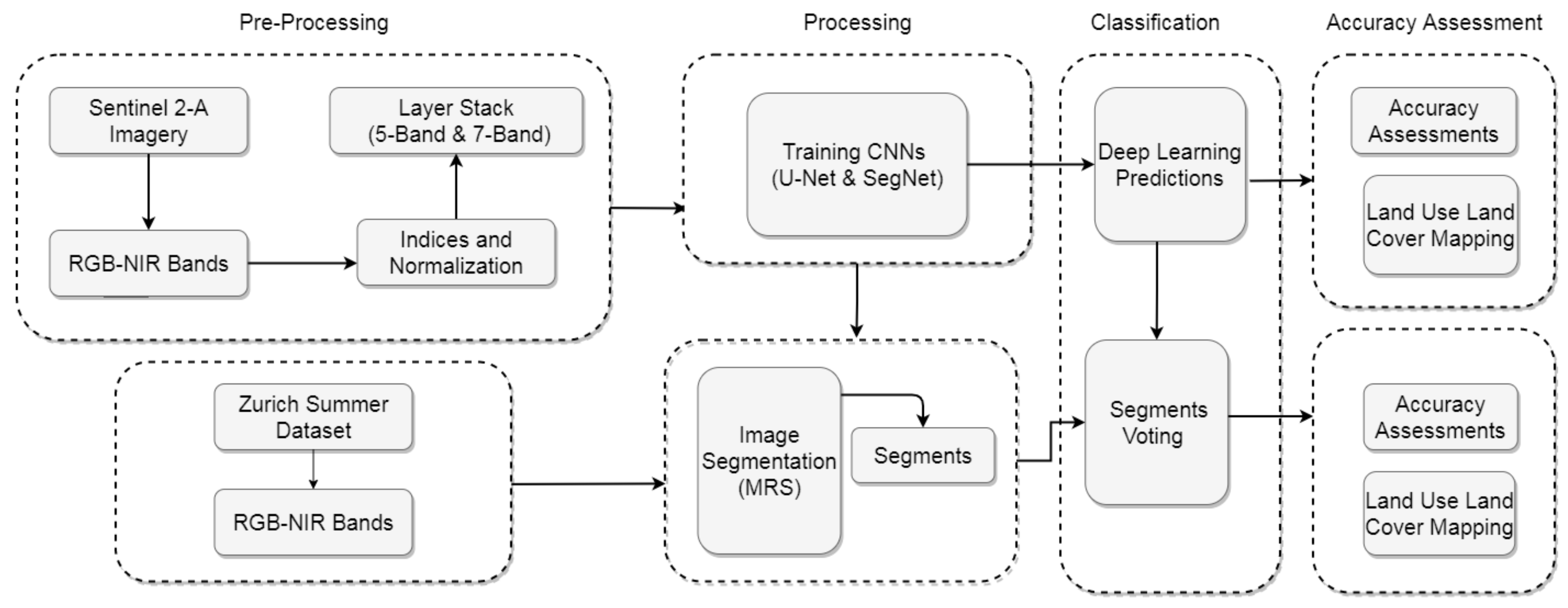
This study aims to produce land cover maps using the CNN-based models combining MRS application to refine the accuracies and automation of the land cover mapping process. The CNN–MRS model consists of two main steps: CNN-based land cover classification and improving the performance of the classification with spatial filter and multiresolution segmentation (MRS). The CNN–MRS model includes the U-Net and SegNet CNN algorithms. Problems such as noise encountered in the pixel-based approach are reduced by the object-based technique. Each of the segments created as a result of MRS is evaluated as an object. The weighted pixel label inside an object is spread over the entire object. The classification accuracy is increased by combining deep learning and multiresolution segmentation.
2. Related Works
In the past, land cover map producing method and accuracy and the data were different from current studies. The National Land Cover Database 1992 (NLCD 1992) for the United States, depending on using multi-temporal Landsat TM, used an unsupervised clustering method with the range of 74% to 85% overall accuracies in NLCD 2001 [7]. In CLC 1990, 2000, 2006, and 2012 from 50 to 25 m, geometric accuracy satellite data were used. In CLC 2018, Sentinel-2 imagery was first used, with ≥85% thematic accuracy. CLC is produced by a visual interpretation by the majority of countries [2]. In recent products, semiautomatic solutions have started to be applied by using in situ data, combining geographic information systems (GIS) with digital image processing, and generalization by a few countries.
In the last decade, the deep learning approach has been effective as a robust method for land cover classification using satellite images [8]. Semantic segmentation of satellite images with CNNs has been conducted for land-cover-based environmental monitoring. There are many tasks completed in this manner, including urbanization [9] and slum areas [10], forestry and vegetation [11], heterogeneous LULC classes [12], and watershed geospatial artificial intelligence (geoAI) applications. There are some large datasets used for segmentation studies, which are also used in several contests such as Deep Globe [13] and Big Net Earth [14]. Numerous challenges are available for image classification on platforms such as Kaggle and CrowdAnalytix to increase the LULC classification accuracy. On the other hand, there are methods such as U-Net and U-CAM, where segmentation accuracies of more than 85% can be achieved using datasets of modest size [15].
Audebert et al. [16] proposed a method that can increase semantic segmentation classification accuracy by using multiple kernels and data fusion from heterogeneous sensors (optical and laser) using CNN architecture. In the same study, the image segments were produced with multiresolution segmentation. NDVI, homogeneity, brightness, and rectangular fit features for each segment were obtained with the help of images from Semarang, Indonesia, and were given as input to deep learning. Another semantic segmentation application in remote sensing was presented by Kemker et al. [17]. Multispectral imagery (MSI) was used in their study, and synthetic MSI data were used using deep convolutional neural networks (DCNNs). Obtained weights were transferred to the real very high-resolution (VHR) MSI data to perform pixel wise classification. Liu et al. [18] proposed combining OBIA and DL and tested with VHR aerial remote sensing images for change detection analysis for natural disasters. In another study [19], Geo Eye-1 and Worldview-1 images were used in CNN architecture. The resulting CNN probabilities were used for object refinement using OBIA segmentation and fuzzy classification to generate sample segmentation of dwellings in a refugee camp. Papadomanolaki et al. used a developed object-based learning framework and compared the results with pixel-based learning using CNN in VHR imagery [20]. Martins et al. presented a framework including OBIA, skeleton-based algorithm usage for object analysis, and conducting several CNNs for land cover mapping using high-spatial-resolution, and the proposed method’s overall accuracy was 87.2% [21]. Another study [22] compared the results of fully convolutional networks, machine learning algorithms, and patch-based DCNN for object-based wetland mapping using unmanned aircraft system images. Li et al. used a methodology that includes an object-based CNN model for LULC mapping with high-resolution imagery [23]. Tuia et al. proposed a model as a region-based analysis for semantic segmentation, and they used spatial regularization and added the region level (related group of pixels) into conditional random fields (CRFs) on VHR satellite and aerial imagery [24].
This study aims to set an example of more automated land cover map production in regional monitoring programs to map scales with less human operator assistance and a convenient approach for updating land cover maps. Classification accuracy for the production of land cover maps was improved by integrating deep learning and object-based approaches. In addition, with the CNN–MRS model, a completely different urban texture was selected as the test area. The classification performance exhibited high accuracy in testing the adaptability to other regions. In most of the studies in the literature where OBIA and deep learning are used together, OBIA results (segments) are given as input to the CNN model. In this study, segmentation was used not as input data for deep learning, but for improving the DL classification results. The CNN-based land cover classification contains the salt–pepper effect, as it is pixel-based. Relevant pixels are grouped under segments by using MRS. Thus, the classification result obtained with deep learning is improved by integration with an object-based approach. The CNN–MRS model was applied to a public dataset and compared with the results of other state-of-the-art CNN models for the same dataset.
3. Study Area and Data
3.1. Sentinel Dataset
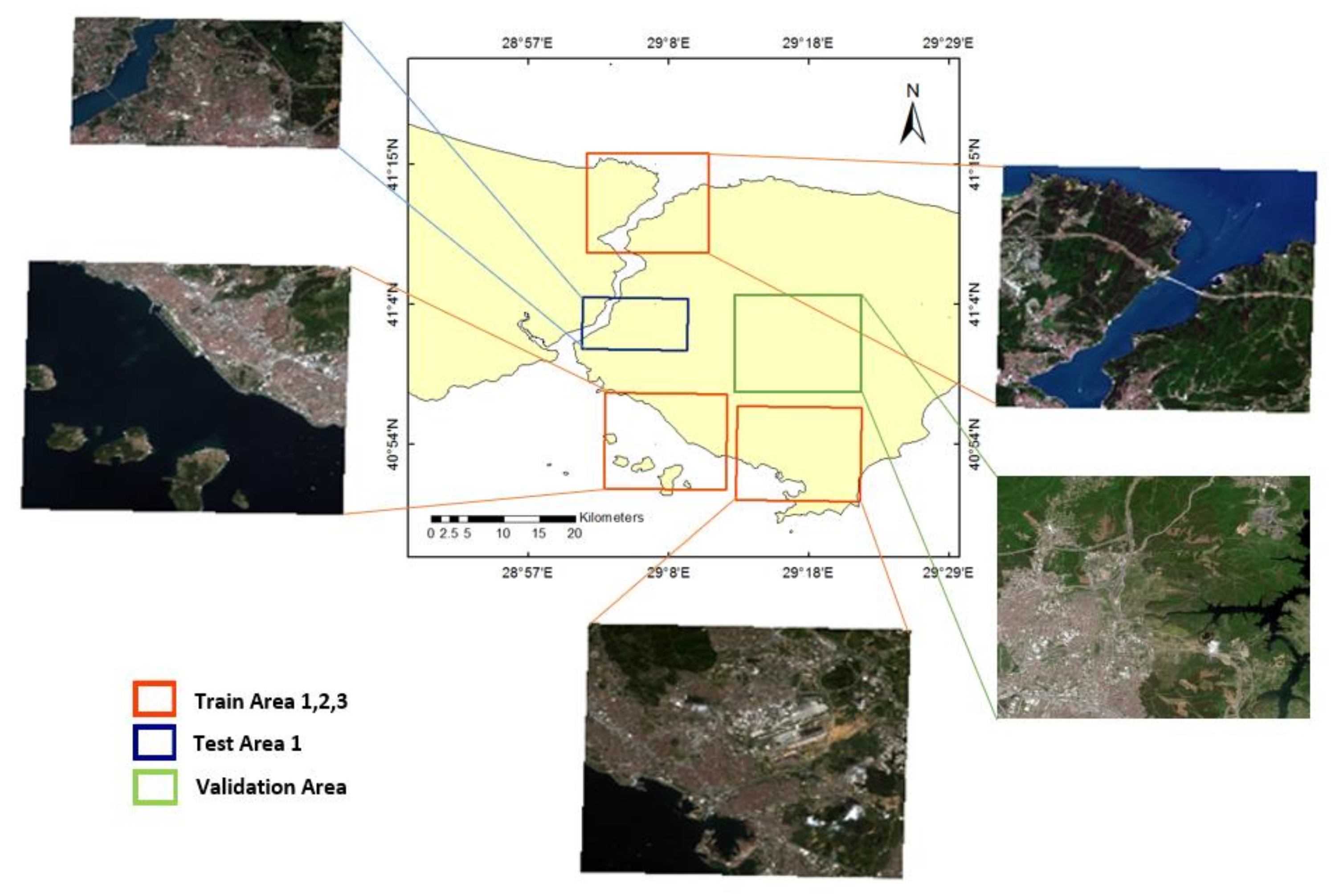
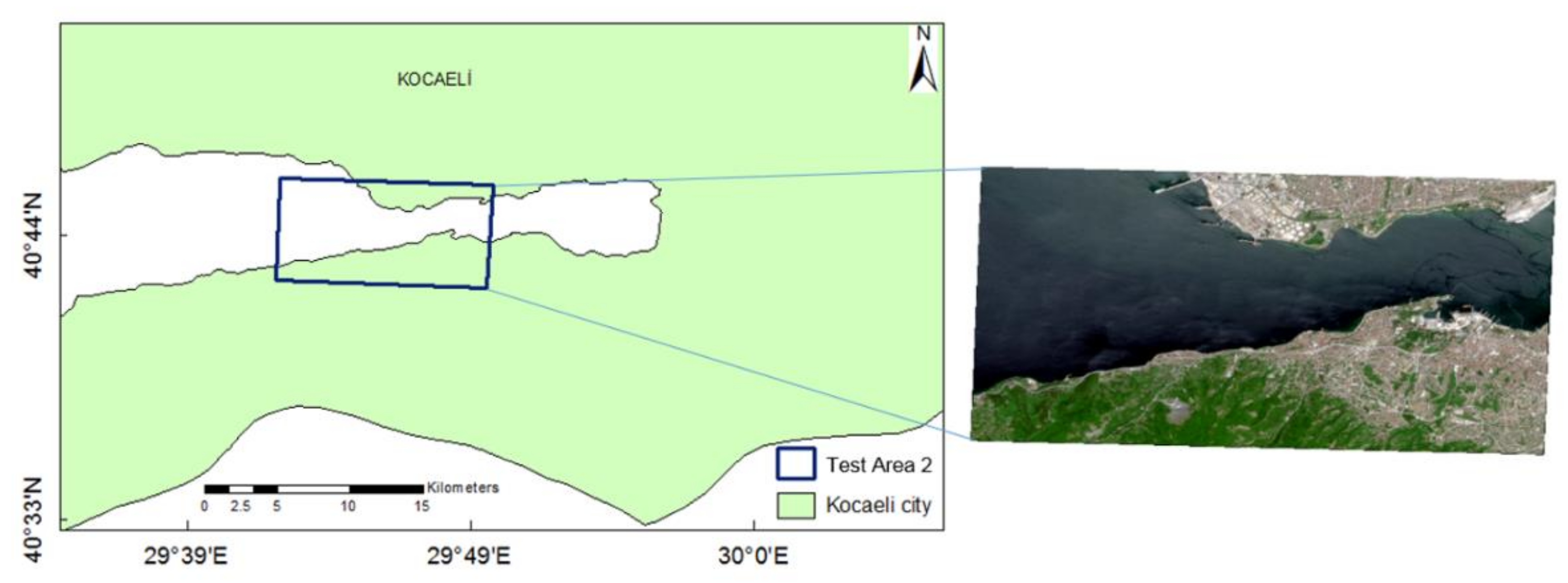
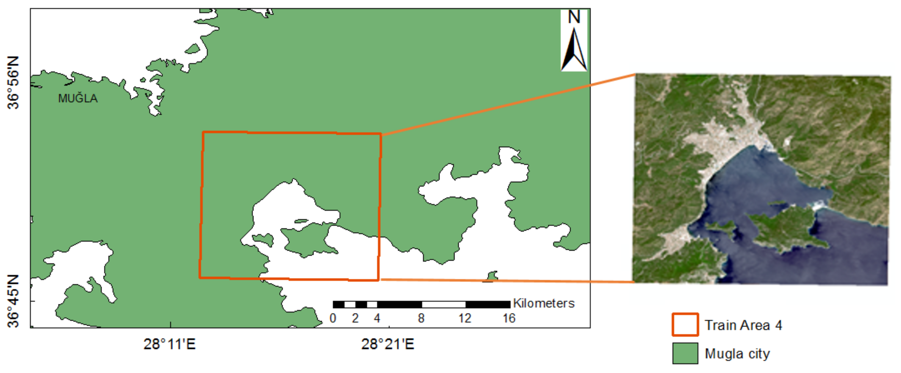
The study site is an approximately 658 km2 area located on the European and Asian sides of Istanbul, the Marmaris region in Mugla, and the nearby Golcuk region in Kocaeli, Turkey (Figure 1). As the study area, regions of approximately equal weight including built-up areas, water bodies, and forest and semi natural areas were selected from three different cities. These cities are located in the northwest and south of the country, so they have different urban and forest texture characteristics due to climate, demographic density, and land use differences. These areas were selected to enable the development of a convenient and adaptable methodology that can be applied to as wide a range of areas as possible, for example, in national map products. Training and testing images were selected separately in these regions. One area in Istanbul (Figure 2) and one area in Kocaeli city (Figure 3) were selected for testing. Three different areas in Istanbul (Figure 2) and one area from Mugla (Figure 4) were selected for training, while an area was selected for validation.
As satellite imagery, input Sentinel-2A imagery was used in the experiment. Sentinel-2 data can be retrieved from Sentinel-Hub (https://scihub.copernicus.eu/, accessed on 21 December 2020) and https://earthexplorer.usgs.gov/ with free access. Sentinel-2A products are ortho-images in UTM/WGS84 projection. The data acquisition date was 24 May 2020 for all satellite images used in this study. Red, green, blue, and near-infrared (NIR) bands were selected for preparing experiment data in 10 m spatial resolution. The images from Sentinel-2, an Earth observation mission from the Copernicus Programme, were used as input data in our study for the following reasons: (i) the satellite’s coverage area is wide (a swath width of 290 km) and used for global acquisitions. (ii) It is a European Space Agency (ESA) mission launched in 2015 and 2017. They provide noncommercial and free data that are multispectral imagery with 13 bands with 443–2190 nm, allowing the production many indices via bands for classifying LULC maps, land monitoring, and various estimations. Sentinel images are quite proper for regional monitoring programs in terms of spatial, spectral, and high temporal resolution (for a single Sentinel-2 satellite, it is 10 days and a combined constellation revisit frequency of 5 days). In deep learning, producing thematic maps with VHR images requires expensive GPU units and computer system requirements. Besides, Sentinel-2 imagery is convenient for thematic map producing requirements and does not require as much heavy processing as VHR images.
The study contains three classes of the first level of LCCS. The artificial surfaces class includes urban fabric, industrial units, dumps, construction, mining sites, and artificially vegetated nonagricultural areas. The forest and semi-natural areas class consists of forests, scrub and herbaceous vegetation associations, and open spaces with little or no vegetation. Water bodies include inland waters and marine waters. All these classes are situated in all training and testing sites.
The classification process follows the commonly used first-level LCCS classes. For instance, in CLC nomenclature, first level thematic maps correspond to 1:100,000 and have a minimum cartographic unit (MMU) of 25 ha and geometric accuracy better than 100 m [1]. Due to the scale used in maps in land cover map production, which includes classes at this level, the images in the dataset to be used in the study were produced with the help of cartographic generalization.
In the study, reference data were manually labeled for all Sentinel-2 images with the visual interpretation method. In visual interpretation, too small regions belonging to different classes were included in the neighboring larger area class. For example, the ships in the sea were included in the water bodies class, not the artificial surfaces class, and ground truth was prepared. Another example is the small wooded areas among the settlements, which were included in the settlement class, i.e., artificial surfaces, unless they met the condition of sufficient generalization. The class distribution of training data for the Sentinel dataset is presented in Table 1.
3.2. Zurich Summer Dataset
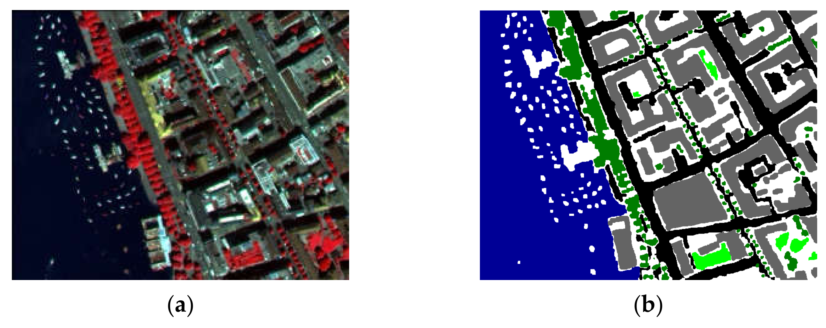
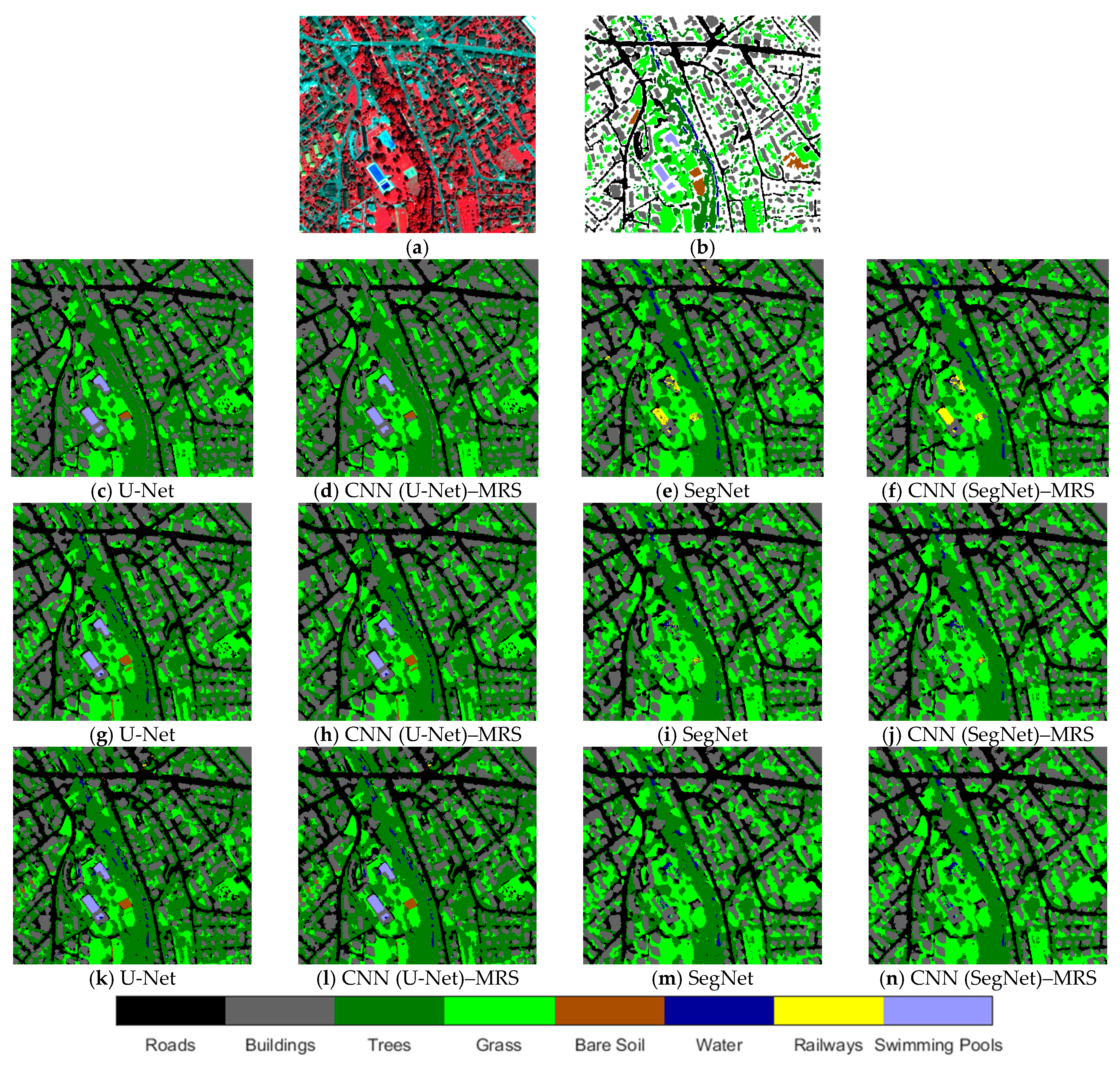
Zurich Summer v1.0 dataset [25] contains 20 cropped QuickBird satellite images with pan-sharpened 0.61 m resolution. The images have four channels (NIR, R, G, and B) and include eight different urban and periurban classes. The classes are roads, buildings, trees, grass, bare soil, water, railways, and swimming pools. A sample image is shown in Figure 5. The dataset class distribution is unbalanced, similar to the real world. The images have approximately 23 million pixels. In the experiment, the ZH-16 and ZH-17 images were used as test images and the ZH-20 image was used as validation data; other images were used in the training.
4. Methodology
Two different experiments were designed in the study. Sentinel data were used in the first experiment. The study area was selected from Istanbul, Mugla, and Kocaeli cities in Turkey. In this experiment, Sentinel-2A images were used. Sentinel-2A bands and spectral indices produced from the bands were stacked. Two different combinations were used as Sentinel datasets. The first dataset included five bands (R, G, B, NIR, and NDVI). The second dataset contained seven bands (R, G, B, NIR, NDVI, SR, and DVI). Additionally, the effect of the size of the input images used on the classification was examined.
In the second experiment, the CNN–MRS model was applied to the Zurich Summer public dataset. At the end of the experiment, the results of the Zurich dataset were compared with other state-of-the-art CNN models.
In the experiments, patch sizes of 32 × 32, 64 × 64, and 128 × 128 pixels were used. The results are shown in the form of tables and land cover maps. In Figure 6, the flowchart of the proposed CNN–MRS model is presented.
4.1. Convolutional Neural Networks
When the feature that can learn from the data is added, rule-based systems can function like classical machine learning. Representation learning can be applied by adding more layers with the feature of learning from data. Representation learning allows AI to adapt quickly to new tasks with less human intervention [26]. Specialized architectures for computer vision tasks are named convolutional networks. CNNs include many convolutional layers that are responsible for understanding the input data specifications. Convolution layers apply filters to the image to extract low- and high-level features in the image. A featured image is obtained, and this identifies a feature type by applying the first filter. Then, a second feature image uses a second filter that detects another feature type. In addition, most machine learning algorithms contain settings called hyperparameters that help control the algorithm’s behavior [26]. While the models are set and used, overfitting or underfitting are undesirable situations. The data used with a convolutional network usually consists of multiple channels. Our study input data have multiple channels as different image bands as well.
Another critical point to consider regarding neural networks is deciding on the architecture to be used [26]. Many different CNN models have been created with different combinations (convolutional layer, pooling, RELU activation, etc.). In this study, experiments were carried out using different architectures as CNN models. While some recent studies try to find an automated framework for datasets with optimum CNN architecture, transferability to other tasks (e.g., dwelling detection) is not apparent [19]. Therefore, determining the optimal CNN model and hyperparameters of the convolution can be changeable according to the case studies.
4.1.1. SegNet
SegNet [27] is a fully convolutional neural network architecture that gives the resolution of prediction output for pixel wise classification in the same way as the input image. The network includes the encoder–decoder layers, convolution layers, batch normalization, pooling indices, and rectified linear unit (ReLU) parts. There is symmetry in the structure of the downsampling and upsampling sections. Finally, the network produces the segmentation result with the softmax layer. This architecture is illustrated in Figure 7.
Each network of encoders and decoders generates a bank of filters to create and batch normalize feature maps. After that, the ReLU layer implements an activation function. The ReLU layer is followed by a max-pooling layer with a 2 × 2 core size. A multiclass classifier named softmax (Equation (1)) is used in the final decoder network to create possibilities to classify each pixel in the image [28].
where n refers to the number of classes, x is the output vector of the model, and index i is in the range of 0 to n − 1. In this study, weights of the VGG-16 [29] model were used as the initial weights.
4.1.2. U-Net
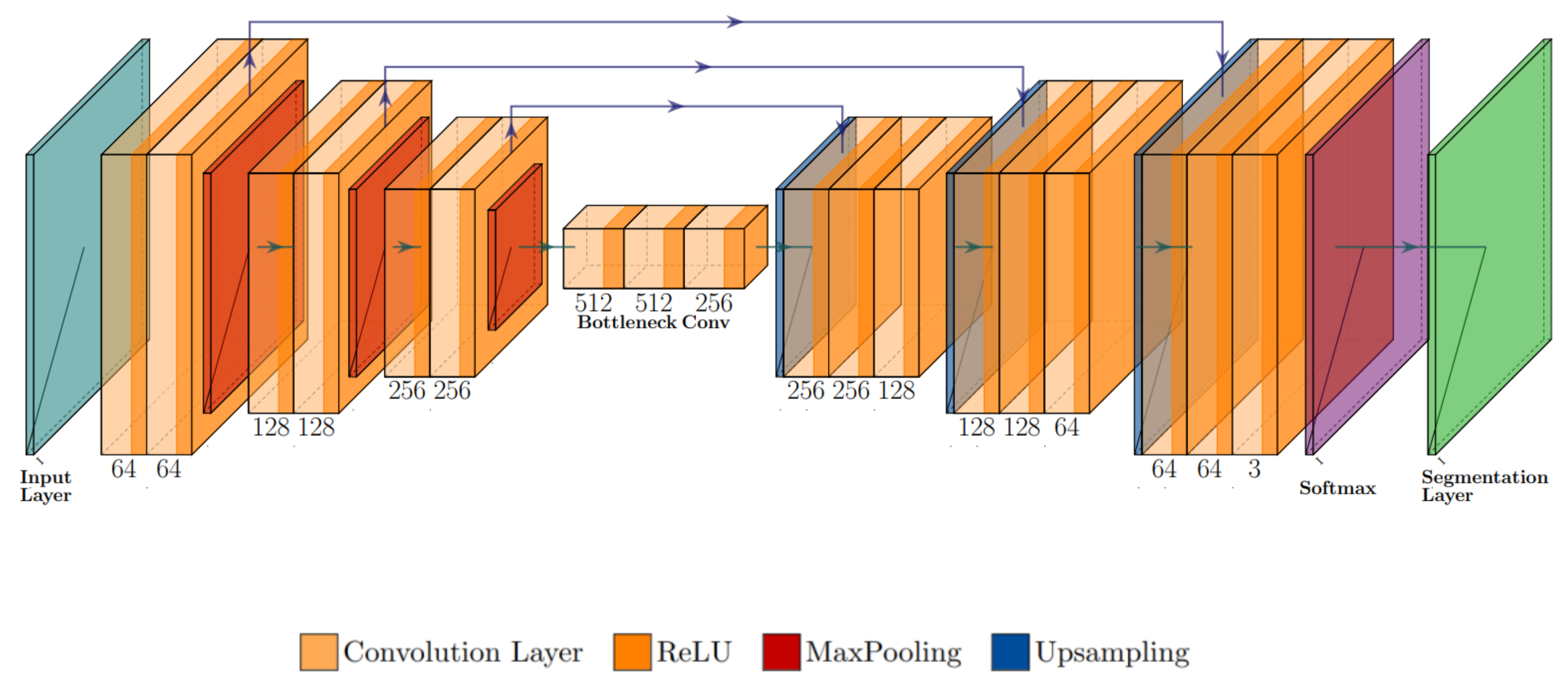
U-Net [30] architecture, which has 23 convolutional layers, includes multichannel feature maps and has a contracting path and an expansive path. There is the repetition of two 3 × 3 convolutions, with a ReLU operation and a 2 × 2 max-pooling part after each of them. The significant change in the U-Net architecture is that having many feature channels in the upsampling section enables the network to spread context information to higher resolution layers. As a result, the expansive path is symmetrical to the contracting way and creates a U-shaped architecture. This architecture has yielded good performance in various biomedical segmentation experiments [30]. It has a wide usage for many computer vision segmentation tasks due to working with very few training data and still yielding precise segmentation results. The generic U-Net architecture illustration is shown in Figure 8.
The general framework of the U-Net model consists of a 3 × 3 window size convolution layer followed by a 2 × 2 window size downsampling layer series. During the convolution process, the activation function (Equation (2)), a transformation function, is used.
where w refers to weight vector, b is bias vector, and is the input of the activation function and the output of convolution operation [28].
4.2. Multiresolution Segmentation
The multiresolution segmentation (MRS) algorithm proposed by Baatz et al. [31] is an alternative to pixel-based image processing algorithms. In the literature, MRS has been a widely used segmentation algorithm [32]. The MRS technique is based on spectral properties; segmentation is the method of separating images into parts. Segmenting an image into objects, extracting features from the objects, and then handling the required interpretation of the image by classifying the features is the main idea of this approach [33]. It can develop more descriptive attributes such as shape, texture, and contextual details by segmenting an image into meaningful objects as an alternative to pixel-based algorithms [34]. Image segmentation, whose purpose is to produce image objects appropriate for further classifications of spatial properties and context, is a key component of object-based image analysis (OBIA) [19]. In the multiresolution segmentation algorithm, the grouping of similar pixels into objects is determined according to the adjustable spectral values of the image layers and the scale, shape, and compactness. The growth of the regions can be limited by using parameters. The algorithm includes a merging process to minimize the average heterogeneity of image objects weighted by the size [34]. Thus, by the local mutual best fitting rule, the pixel groups are merged as segments. Shape and color weight values complement each other, and their sum is equal to 1. Similarly, the sum of compactness and smoothness values is 1, and these values individually change between 0 and 1. The merging cost function integrates spectral and shape heterogeneity, as shown in Equation (3) [33].
where w belongs to weight for spectral heterogeneity with the interval 0–1; and refer to shape and color parameters, respectively. In many studies, multiresolution segmentation was applied [35,36,37,38,39,40]. The algorithm has a widespread effect in remote sensing applications, and its use is continuing.
4.3. Majority Voting
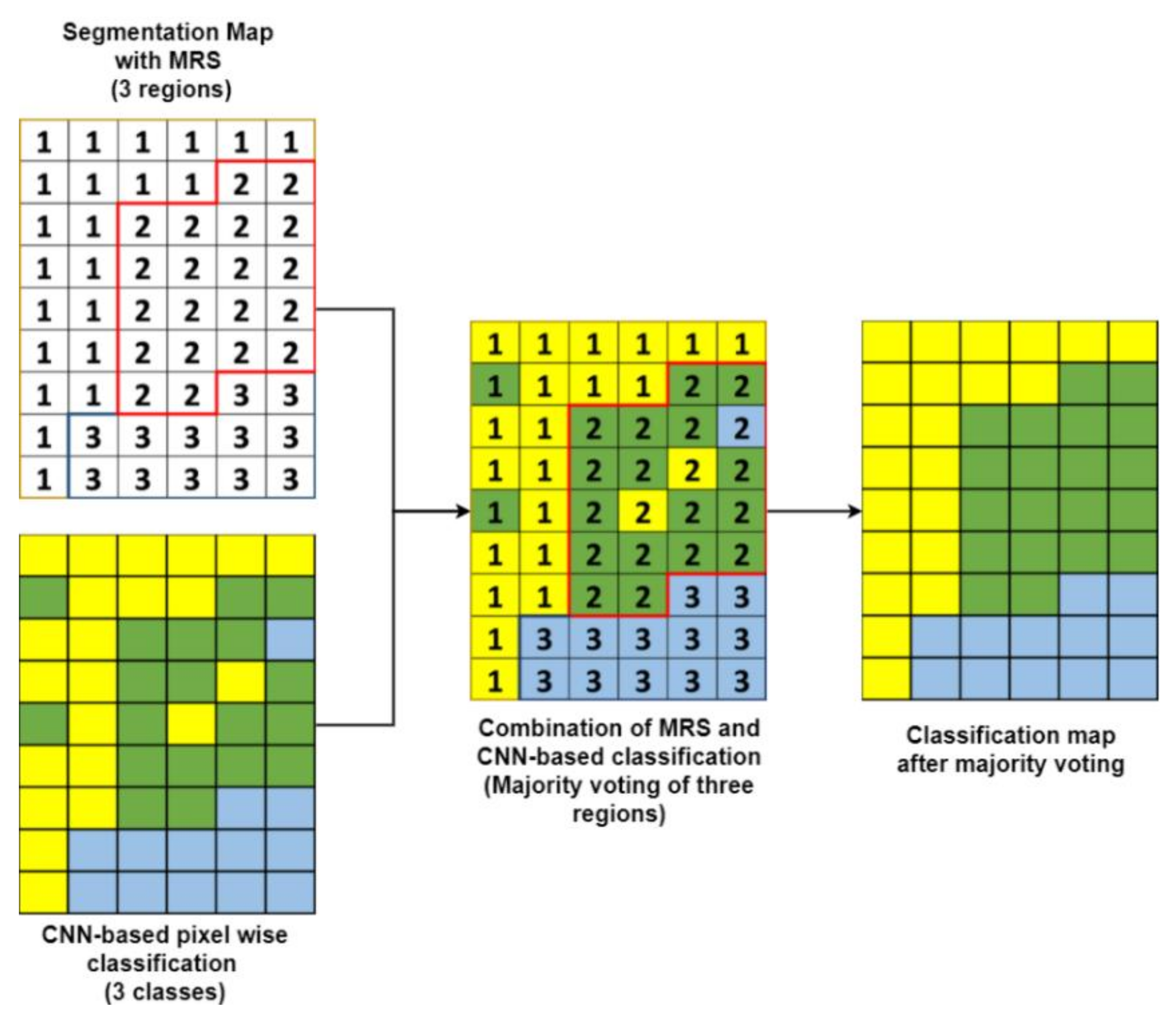
In the CNN–MRS model, class category is voted for by pixels in each object, which is segmented by MRS. The images are separated as objects by MRS. A segment includes n number pixels. Each pixel has a class category (Catc) after semantic labeling with semantic segmentation. A general mathematical model with formulas is shown in Equations (4)–(6). Labeled categories, Catc, are shown in Equation (4).
Catc = Cat 1|| Cat 2||,…,|| Cat k
Catm is a new category determined for the object, and k is the threshold value for determining the decision of the majority ratio. refers to the majority category for the object. It is calculated for each object of the MRS results. If an object cannot make the majority in a category with the specified k value, the classes of all pixels in that object will remain the same. Therefore, this application represents a category calculation made for each object. Each pixel in the object takes the new category value of the object it contains. Thus, CNN-based classification is refined by MRS-based majority voting (Figure 9).
4.4. Spectral Indices
Sentinel-2A images have 13 different spectral bands with various spatial resolutions. VNIR bands have 10 m spatial resolution. Many studies have shown that using indices as features in the classification can increase accuracy, especially according to the related classes. In this study, spectral indices and band ratios were used in CNN models with two combinations. These indices are normalized difference vegetation index (NDVI), differential vegetation index (DVI), and simple ratio (SR) (Table 2). These indices are beneficial for distinguishing green leaf objects generally. Besides, in this study, the water bodies class was distinguished from others well. Thus, there was no need to use indices for the water bodies class. These three selected indices helped to differentiate artificial surfaces from the forest and seminatural areas class. The effect of indices on classification was also investigated in this study. In the experiment, the five-band dataset includes VNIR bands and NDVI index, and the seven-band dataset includes VNIR bands and NDVI, DVI, and SR indices as layer stacking.
4.4.1. Normalized Difference Vegetation Index (NDVI)
In NDVI, healthy vegetation absorbs more red light in the visible area, while unhealthy vegetation has higher reflectance than healthy vegetation. NDVI values range between −1 and 1. NDVI is also used for drought monitoring worldwide and has fairly widespread use. NDVI is a good indicator for differentiating vegetation from artificial areas. It was used in both the five-band and seven-band datasets in the study.
4.4.2. Simple Ratio (SR)
Simple ratio (SR) is a spectral ratio index that is calculated with the ratio between reflectance recorded in the NIR and red bands. It is used for distinguishing objects that have green leaves from other objects in the images. Green leaf objects have low reflectance values in the red region but higher reflectance in the NIR region of the sensors. It is expected that soil regions and bare lands would have SR values of almost 1, but green leaf objects would have SR values much greater than 1. In addition, the SR index can be used to estimate the relative biomass in images.
4.4.3. Differential Vegetation Index (DVI)
Infrared and red band difference [44] as a vegetation index can differentiate between soil and vegetation regions. DVI was used in the seven-band dataset. The index may help separate impervious surface and non-cultivated soil areas, giving a similar result with SR as another related study example. Impervious surface regions belong to the artificial surfaces class, but non-cultivated soil areas belong to the forest and semi natural areas class in the study.
4.5. Accuracy Assessment and Classification Results Comparison
Standard accuracy assessment parameters for class metrics, namely precision, recall, F1-score, and intersection over union (IoU) (Equations (7)–(10)) were computed for the predicted images using metrics of true positive (TP), false positive (FP), and false negative (FN) [45]. Overall accuracy (OA) [46] and kappa [47] were evaluation metrics for the classification (Equations (11) and (12) [48]).
TP is when the prediction and example are positive. FP is when the prediction is positive but the example is negative. FN is when the prediction is negative but the example is positive. TN is the prediction and example are negative. IoU is calculated for all classes separately, and it is equal to the ratio of correctly classified pixels to the total number of ground truth and the predicted pixels. OA is an estimation of the percentage of correctly classified pixels. Av. F1 is the average of F1-score [49] of all classes that were calculated in all images.
One of the methods used to test whether the values or findings obtained from research are statistically significant is the McNemar test [50]. The statistical significance of the difference between the two proportions can be measured using McNemar’s test for dependent variables. The McNemar test depends on the chi-square distribution and uses a 2 × 2 dimensional error matrix in calculations [51]. In thematic mapping studies with the image classification method, accuracy assessment is conducted for different classifiers first. Then, the statistical significance of the difference between the accuracy calculations can be determined using the kappa coefficient and McNemar test [51]. The calculation of McNemar test value is shown in Equation (13), where f21 indicates the number of samples that were classified incorrectly (i, j = 1, 2) and a value is obtained.
For this analysis, 2 × 2 contingency tables (Table 3) were calculated by using the study’s results of each model and reference data for different test sites. When H0 hypothesis is accepted, that means two different methods do not have a significant difference. If the value of calculated χ2 is greater than the value of χ2 in the table, the H0 hypothesis is rejected. If the value of χ2 found by calculation is lower than the value of χ2 in the McNemar test table, the H0 hypothesis is accepted. Table values are constant; e.g., for 95% accuracy confidence; the table value is 3841. If the null hypothesis H0 is true, paired models are the same, or neither of the two models performs better than the other one. Thus, when H0 is true, it means the two methods do not have a significant difference. On the other hand, if the H1 hypothesis is true, there is a significant difference between the two models.
4.6. Experiment
In the first experiment, spectral indices (NDVI, DVI, and SR) were used for layer stacking in two combinations of Sentinel-2 bands. Five-band layer stacking included B4, B3, B2, B8, and NDVI. Seven-band layer stacking was obtained by adding two more indices: DVI and SR. All bands have a normalized interval with zero-center normalization in the image input layer of the algorithms. Zero-center normalization typically means that images are normalized with a mean of 0 and a standard deviation of 1.
In the Sentinel dataset, the training data consisted of three images of 1311 × 1287 pixels. The validation data consisted of an image of 1311 × 1287 pixels. Two testing data images were each 689 × 1101 pixels. The Sentinel dataset contained approximately 17% validation, 15% testing, and 68% training data. In CNN-based deep learning models according to the different patch sizes, proper batch sizes were set. CNN sample patch window refers to patch size, and it is an example of a convolution input sample. In this experiment, 128 × 128 patch size was determined as 16 batch size, 64 × 64 patch size as 32 batch size, and 32 × 32 patch size as 128 batch size. Batch size refers to how many data will be processed simultaneously in the DL process. The most suitable batch size parameters were selected according to the hardware features used. Moreover, stochastic gradient descent (SGD) was used as an optimization algorithm. The learning rate is a key parameter for the SGD algorithm [26]. In the experiment, the initial learning rate of 0.01 was applied. For each experiment, different and proper epoch numbers were set for the deep learning-based models.
In the second experiment, on the Zurich dataset, the same workflow was conducted. The dataset was split into testing, training, and validation parts. The obtained results were compared with state-of-the-art models in the literatüre.
The change in the image particle size was also a variable in the learning model, affecting the optimization in selecting other hyperparameters. Thus, optimum epoch numbers were determined experimentally. After hyperparameter determination, two deep learning methods were trained with selected hyperparameters using three different patch sizes (32 × 32, 64 × 64, and 128 × 128). All pixels in the images had labeled class categories according to deep learning-based learning models. Afterward, the classification results of the CNN models were post-processed by applying a median filter and MRS by using the semantic segmentation images. Median filtering is a nonlinear function often used for diminishing noise [52]. The function replaces pixels with the median of neighboring pixels by using a kernel-size window. The literature contains several applications of spatial filter types for LULC tasks [53,54], including to reduce speckle effect and preserve edges. The kernel size of the median filter was selected as 5 × 5 for the Sentinel dataset and 3 × 3 for the Zurich Summer dataset. In the study, the experiments were carried out with a computer with i7 7700HQ 2.8GHZ, 16GB RAM, and GTX1050Ti 4GB graphics card. The experiments were implemented in MATLAB software.
The algorithm of MRS is preferred in the CNN–MRS model to protect feature information of pixels. MRS is the first step of object-based image classification (OBIA) applications. In experiments, MRS was performed using eCognition Developer v.9.3, and the images were divided into segments including a seven-band stack image. MRS was performed with 65 scale, 0.3 shape, and 0.5 compactness parameters for the Sentinel dataset and 65 scale, 0.4 shape, and 0.5 compactness parameters for the Zurich Summer dataset. Thus, semantically related objects were generated to be used instead of pixels. The pixels labeled with CNN were relabeled according to the category of the major class within the segments generated as a result of MRS, and the pixels in the segment were combined under a single class. Since pixels belong to different classes in the segment, the optimum threshold value for determining the major class was experimentally determined as 40% for the Sentinel dataset and 80% for the Zurich Summer dataset.
5. Results
5.1. Segmentation Quality Assessment
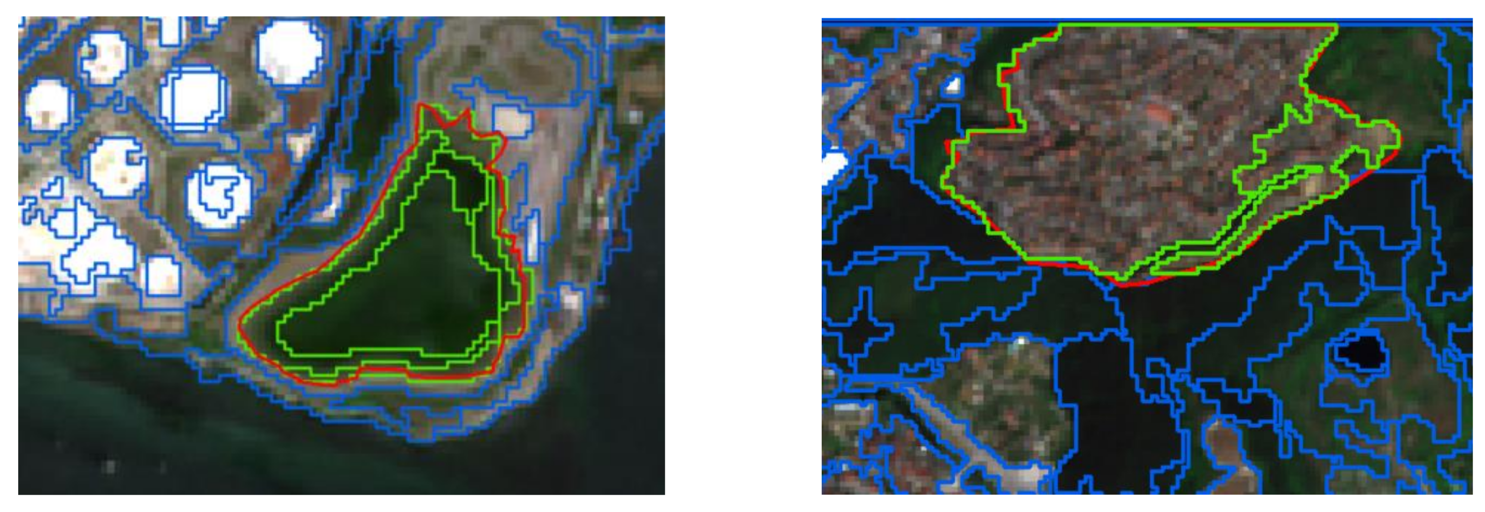
Multiresolution segmentation parameters are determined experimentally. There are some parameters in the literature to evaluate segmentation quality. The most used parameters are segmentation anomalies known as undersegmentation (US) [55] and oversegmentation (OS) [55] (Equations (14) and (15)). The division of the real object into more than one small subsegment is called oversegmentation, while part of the real object becoming part of another object is called undersegmentation [56]. These values are calculated as a function of the reference object area (Ar) and the object area obtained as a result of segmentation (As). In this study, US, OS, root mean square (RMS) [55], area fit index (AFI) [57], and quality rate (QR) [58] were used as segmentation quality metrics (Equations (16)–(18)). In good segmentation, US, OS, RMS, and AFI are expected to be 0 and the QR value is expected to be 1. Quality metrics were calculated for each test image. Some subsets of the test image are shown in Figure 10 and Figure 11.
According to segmentation quality metrics, the Sentinel dataset has better segmentation quality than the Zurich Summer dataset. The most important reason for this is the difference in resolution and the number of classes. As the resolution and the number of classes decrease, the segmentation quality increases. Because high-resolution images contain more details, the probability of objects mixing with each other is high. The segmentation quality metrics for both datasets are shown in Table 4 and Table 5.
5.2. Experimental Results for Sentinel Datasets
Deep learning-based scene classification and the proposed methodology using the CNN–MRS model were applied to the two different test site areas with five- and seven-band stack images. These processes were achieved for three different patch sizes: 32 × 32, 64 × 64, and 128 × 128. The optimum patch size for each model in the experiment was searched for.
The Istanbul city test area is approximately 75 km2, representing the most cosmopolitan city in the country. This first test area was selected from the same city as the three training images.
Table 6, Table 7, Table 8, Table 9, Table 10, Table 11, Table 12 and Table 13 show artificial surfaces class (AR), forest and semi-natural areas class (FSN), and water bodies class (WB). Overall accuracy (OA) and average F1-score (Av. F1) are also shown.
According to the five-band dataset results for the Istanbul city test site, the highest overall accuracy value was obtained with the CNN–MRS model with U-Net model patch size of 64 × 64 as 97.31% (Table 6). The lowest overall accuracy for the Istanbul test site was obtained with the SegNet model with a patch size of 128 × 128 as 79.41% (Table 7). The best performance for individual class F1-score was obtained with the CNN (U-Net)–MRS model with 64 × 64 patch size in the experiment for the water bodies class as 98.43% (Table 6). The worst F1-score was obtained by the SegNet model patch size 128 × 128 for forest and semi-natural class as 51.36% (Table 7). The best per-class score of IoU was found for the CNN (U-Net)–MRS model with 32 × 32 patch size for waterbodies class as 99.51% (Table 6). The lowest value of IoU was found for the SegNet model with 128 × 128 patch size for forest and semi-natural areas class as 53.67% (Table 7). Generally, artificial surface performance values for the models are at a modest level. It is also discernible in the semantic segmentation results that all CNN–MRS model results are better than the state-of-the-art CNN-based models.
In the Istanbul test site area, it is noticeable for the seven-band dataset that the best performance was obtained with the CNN (SegNet)–MRS model with 128 × 182 patch size as overall accuracy of 97.09% and kappa of 94.40%, and the CNN (U-Net)–MRS model with 32 × 32 patch size had an average F1-score of 94.68% (Table 8 and Table 9). Again, the same model yielded the best scores for artificial surfaces and forest and semi-natural areas classes as class metrics. The best performing model for the water bodies class is the same model with the 128 × 128 patch size. The worst performance results were found for the SegNet model with 32 × 32 patch size for overall accuracy at 89.23%, average F1-score at 71.74%, and kappa coefficient at 80.12% (Table 9).
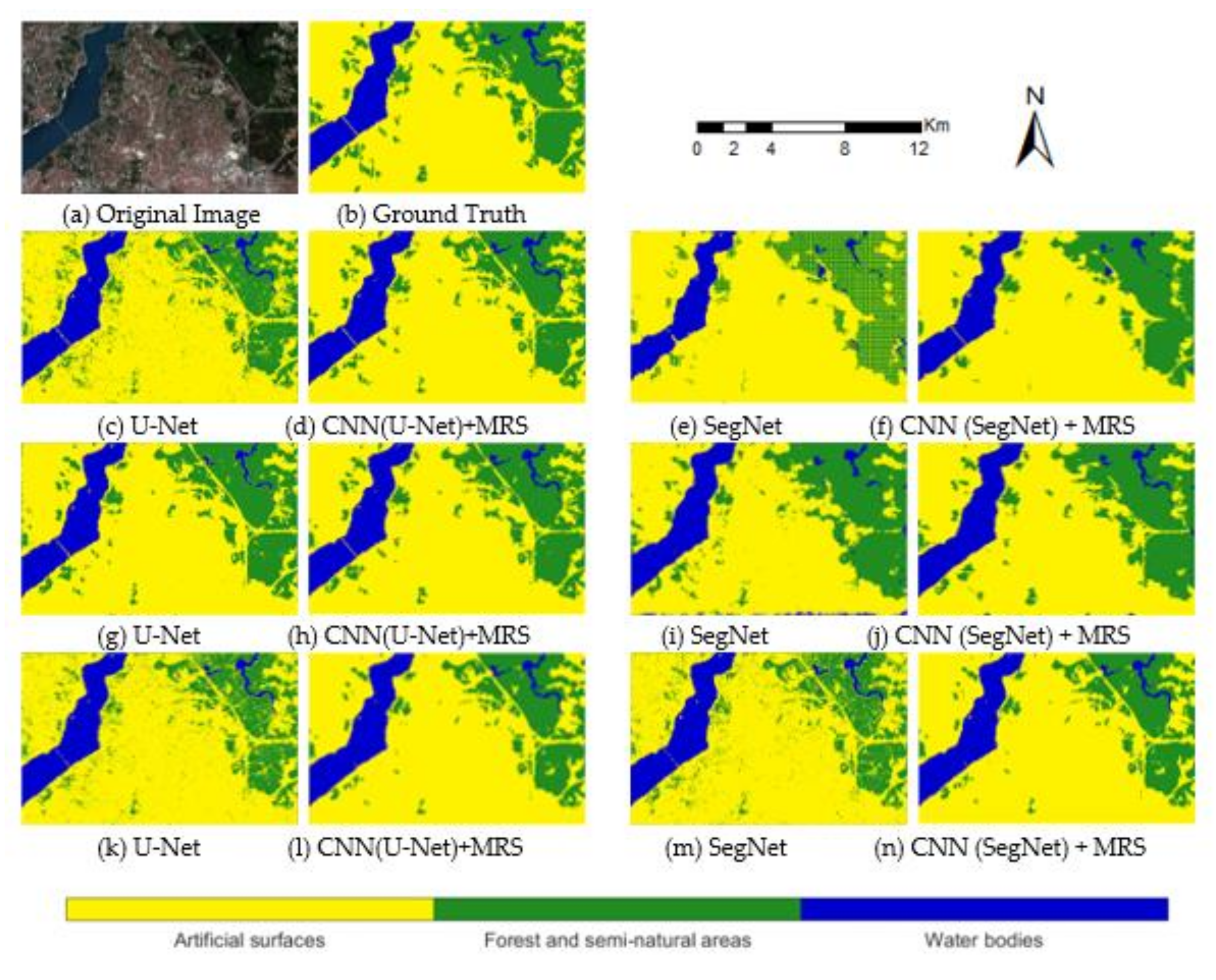
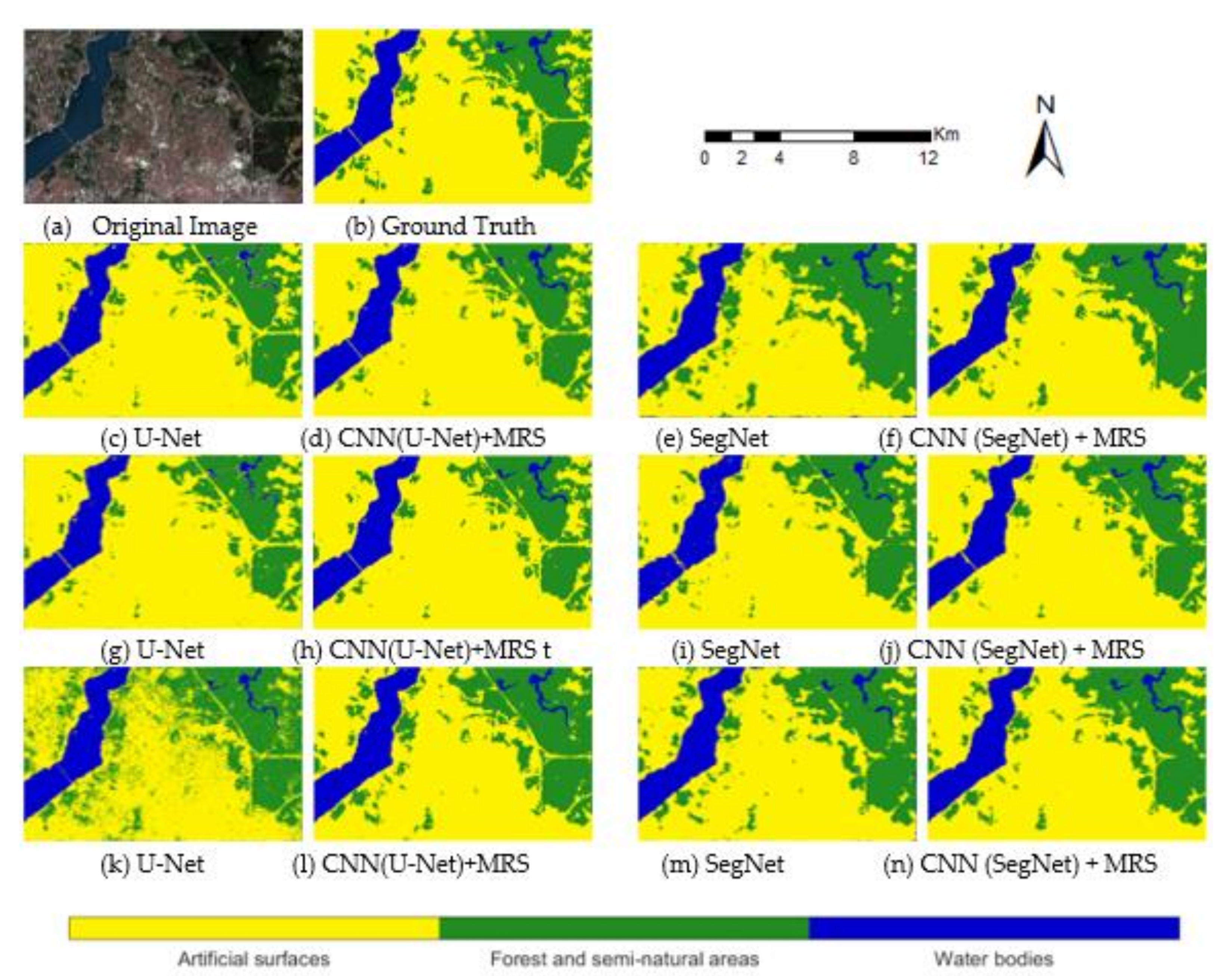
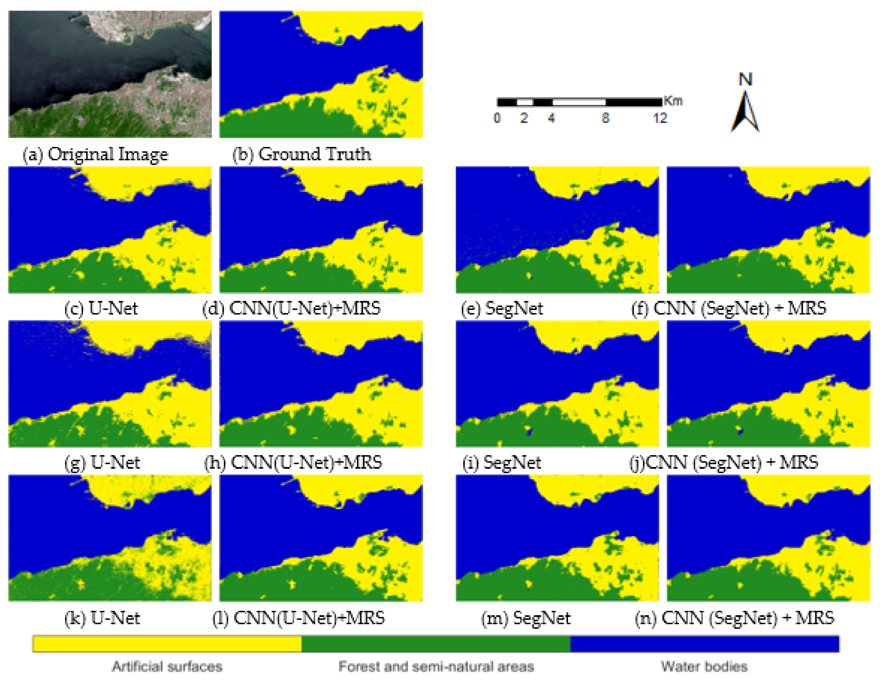
The classes were predicted better with the CNN–MRS model than with state-of-the-art CNN models. Notably, for the U-Net model with 128 × 128 patch size, the result has a strong salt–pepper effect (Figure 12). The CNN–MRS model used for this model helped to improve the results greatly. The bridge over the Bosphorus as an artificial surface class has disappeared in the results of some models. The bridge was segmented by CNN (U-Net)–MRS model with 32 × 32 and 64 × 64 patch sizes and CNN (SegNet)–MRS model with 64 × 64 patch size. Land cover classification results of five- and seven-band datasets for the Istanbul test site area are shown in Figure 12 and Figure 13, respectively.
The other test area was selected in different cities from the training areas. Thus, the usability of the trained models in different test areas was investigated. The Kocaeli test area results were comparable to those of the Istanbul test site. In Kocaeli, the highest overall accuracy result was found for the CNN (U-Net)–MRS model with five-band dataset and 32 × 32 patch size as 98.44% (Table 10). The lowest accuracy result was found using the SegNet model 32 × 32 patch size of the five-band dataset as 89.85% (Table 11). Likewise, in the accuracy assessment tables, the prediction figures found the recognizable differences in the results of the Kocaeli test site models with the five-band dataset (Figure 14). The harbor is generally minimalized or absent in semantic segmentation results with SegNet and CNN (SegNet)–MRS models. The most successful method in terms of overall accuracy for artificial surfaces and forest and semi-natural areas classes is CNN (U-Net)–MRS model using 32 × 32 patch size.
In the Kocaeli test site area, CNN (SegNet)–MRS models using 64 × 64 patch size had the highest scores for all evaluation metrics (except IoU value of the forest and semi-natural areas class). Finally, through these results, it is revealed that the results of state-of-the-art models based on CNNs are improved by using the CNN–MRS model. The worst values were obtained with SegNet model with 32 × 32 and 128 × 128 patch sizes. Moreover, there is no optimum CNN-based model. It varies according to the dataset and test site area.
The observable semantic segmentation results are shown for Kocaeli test site area with the seven-band dataset (Figure 15). There are considerable differences between this dataset and the five-band dataset for this region with the same models. In this experiment, our CNN (SegNet)–MRS model with 64 × 64 patch size yielded superior results compared to other models. U-Net models obtained more detailed results, and this caused a stronger salt–pepper effect in some patch sizes. SegNet models showed more smooth class transitions generally.
The best scores are the results of the CNN–MRS models in both class metrics and the aggregate five-band dataset. With overall accuracy at 98.44% and kappa coefficient at 97.44%, the results of our approach with U-Net with 32 × 32 patch size are the highest values (Table 9). For average F1-score, the 64 × 64 patch size with the same model resulted highest at 96.46%. The lowest predicted results of these evaluation metrics were obtained by using SegNet model with the 32 × 32 patch size (Table 11).
For individual classes, F1-score and IoU results are shown as different accuracy evaluation metrics. According to all test results, for separate classes, the best scores belonged to CNN–MRS model performances. The CNN–MRS models were compared quantitatively with mainstream and state-of-the-art CNN-based models (U-Net and SegNet) (Table 8, Table 9, Table 10, Table 11, Table 12 and Table 13). Significant superiority was shown by the CNN–MRS models, which had the best classification performances. The results of the seven-band dataset are shown in Table 12 and Table 13.
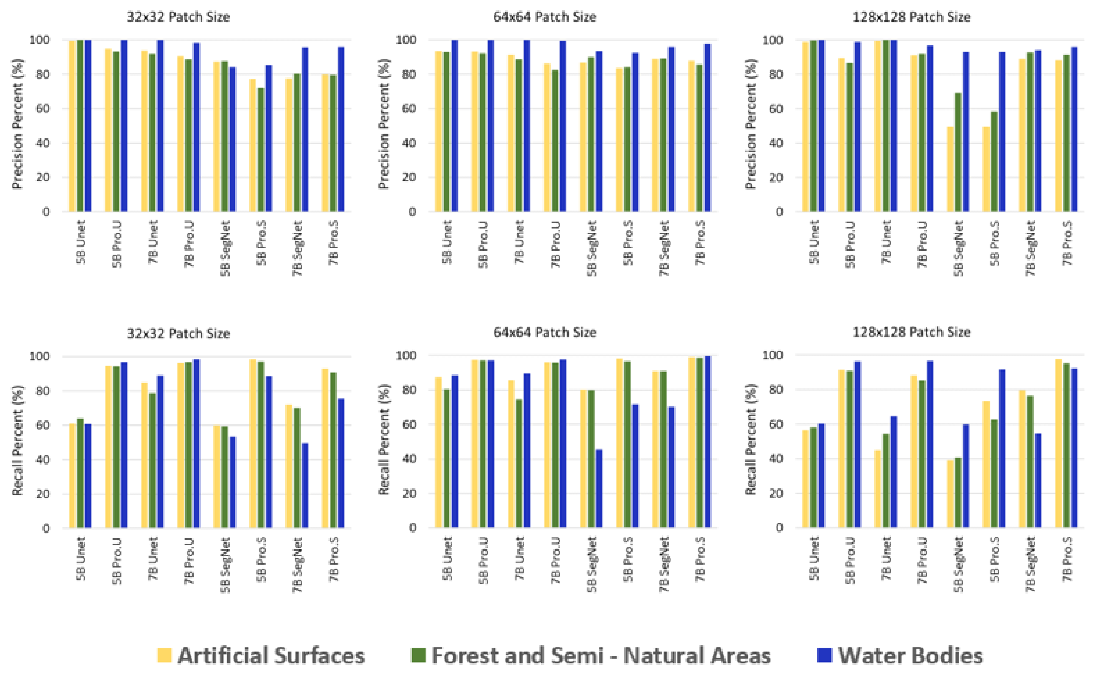
Applying a particular metric for understanding the assessment may not be sufficient in an imbalanced dataset. A more detailed evaluation may be required, especially for models with adaptation purposes. The results of the study were also examined as classification accuracy at the class level. Precision and recall of each class and recall values were calculated for all models with varied patch sizes for two datasets. Moreover, per-class F1-scores and average F1-score of the study also provide some required information about the efficiency of the models.
In general, precision scores for the individual classes were found to be better than recall for both test site areas. In the Istanbul test area, the lowest precision values were found for SegNet using 128 × 128 patch size in the five-band dataset. There is a slight difference in precision between CNN models and the CNN–MRS models. There is a substantial difference in recall between CNN models and the CNN–MRS models. The CNN–MRS model recall outcomes were better than those of state-of-the-art CNN-based models for all experiments.
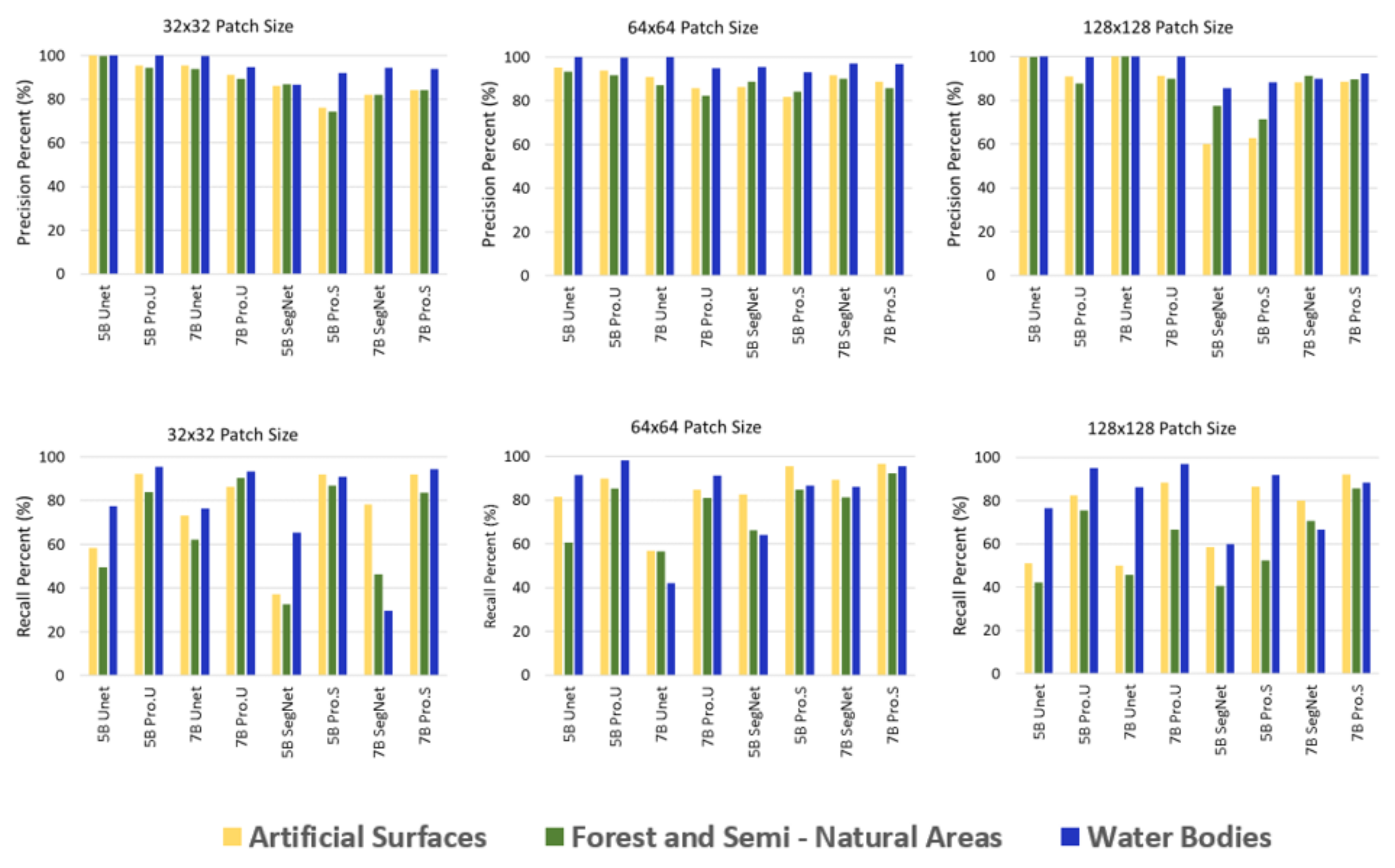
In both five- and seven-band Sentinel datasets, similar precision–recall trends were observed. In general, precision outcomes were better than recall outcomes. Therefore, F1-scores were decisive for the interpretation of this variety. In both test site areas, precision and recall of water bodies class outcomes are better than those of the other two classes. That was an ordinary circumstance because forest and semi-natural areas class and artificial surfaces class are highly nested. Recall values for all classes were increased with CNN-MRS models in İstanbul test area (Figure 16). Precision and recall values for Kocaeli test area were represented in Figure 17.
5.3. McNemar Test
McNemar [59] established several formulas to measure the significance of the difference between two correlated proportions. The McNemar test was used for the experiments of all different methods on five- and seven-band Sentinel datasets. Therefore, the significance of the difference between the accuracies of the land cover classification produced by different methods was statistically analyzed using the McNemar test.
McNemar test is used for paired nominal (categorical) data, and our study data are appropriate for that evaluation. In this study, all paired models correspond to H1 hypothesis. α is the significance level for 95% accuracy confidence. p is a value is calculated with the test. When H1 hypothesis is valid, α = 0.05 significance level for p < α. For all pairs, chi-squared values were calculated and compared to the value of 3841. According to the results, all paired models of our study are significantly different, and the predictive performance of the models is different. It was calculated for five- and seven-band Sentinel datasets for each patch size (32, 64, 128) for the state-of-the-art CNN models and proposed ones. According to the McNemar test, dataset H1 hypothesis for all methods of the Sentinel dataset is true, which means comparing all the methods is significant (Table 14).
5.4. Results for Zurich Summer Dataset
According to the quantitative comparison of the results, CNN–MRS model usage increased the accuracies and performance metrics. Applying the spatial filter and MRS on U-Net and SegNet classification increased the overall accuracies for all patch sizes. The highest evaluation metrics belong to SegNet–MRS models (Table 15 and Table 16). These refinement values of the proposed approach are also compatible with the experiments conducted on the Sentinel dataset (Table 9, Table 11 and Table 13).
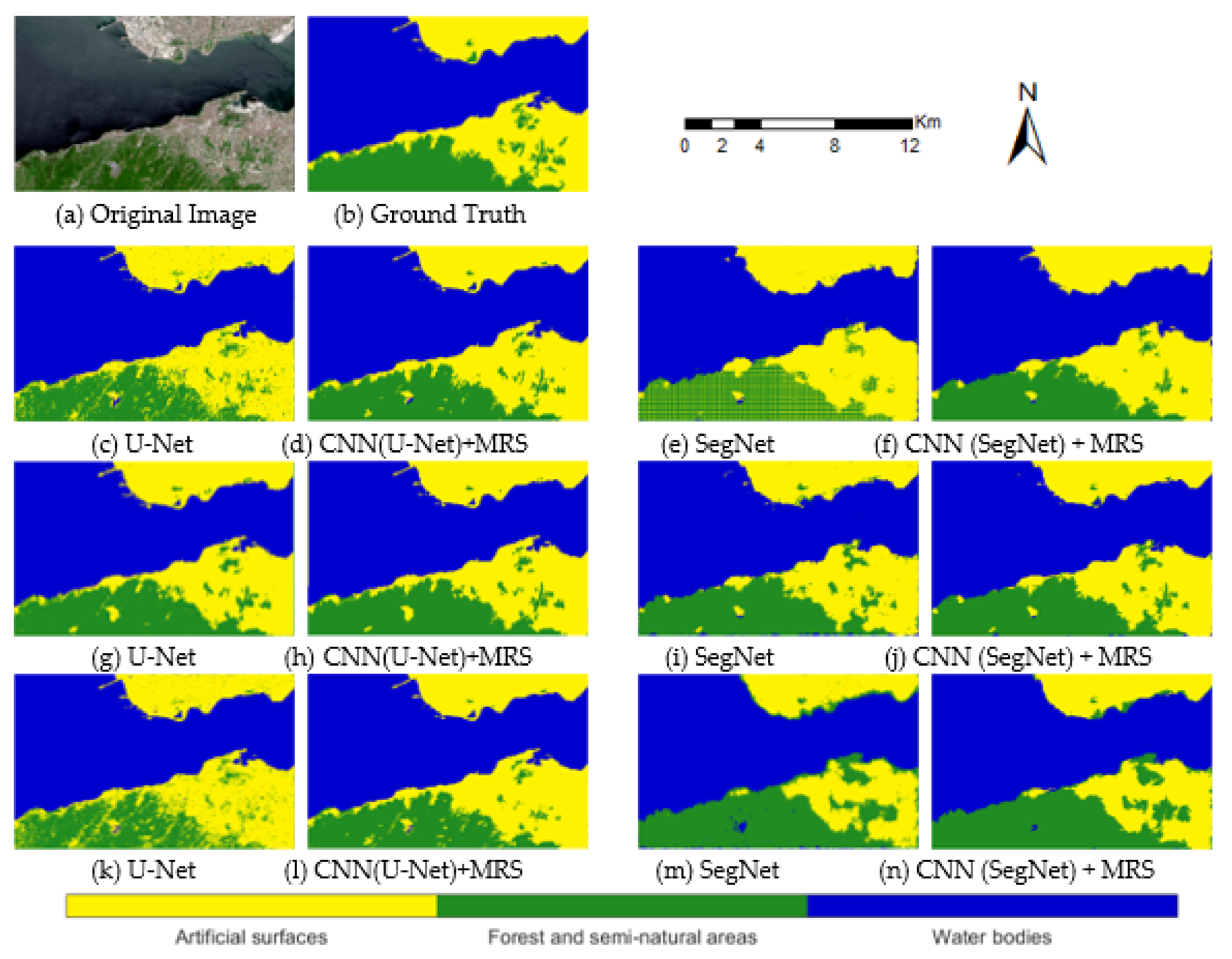
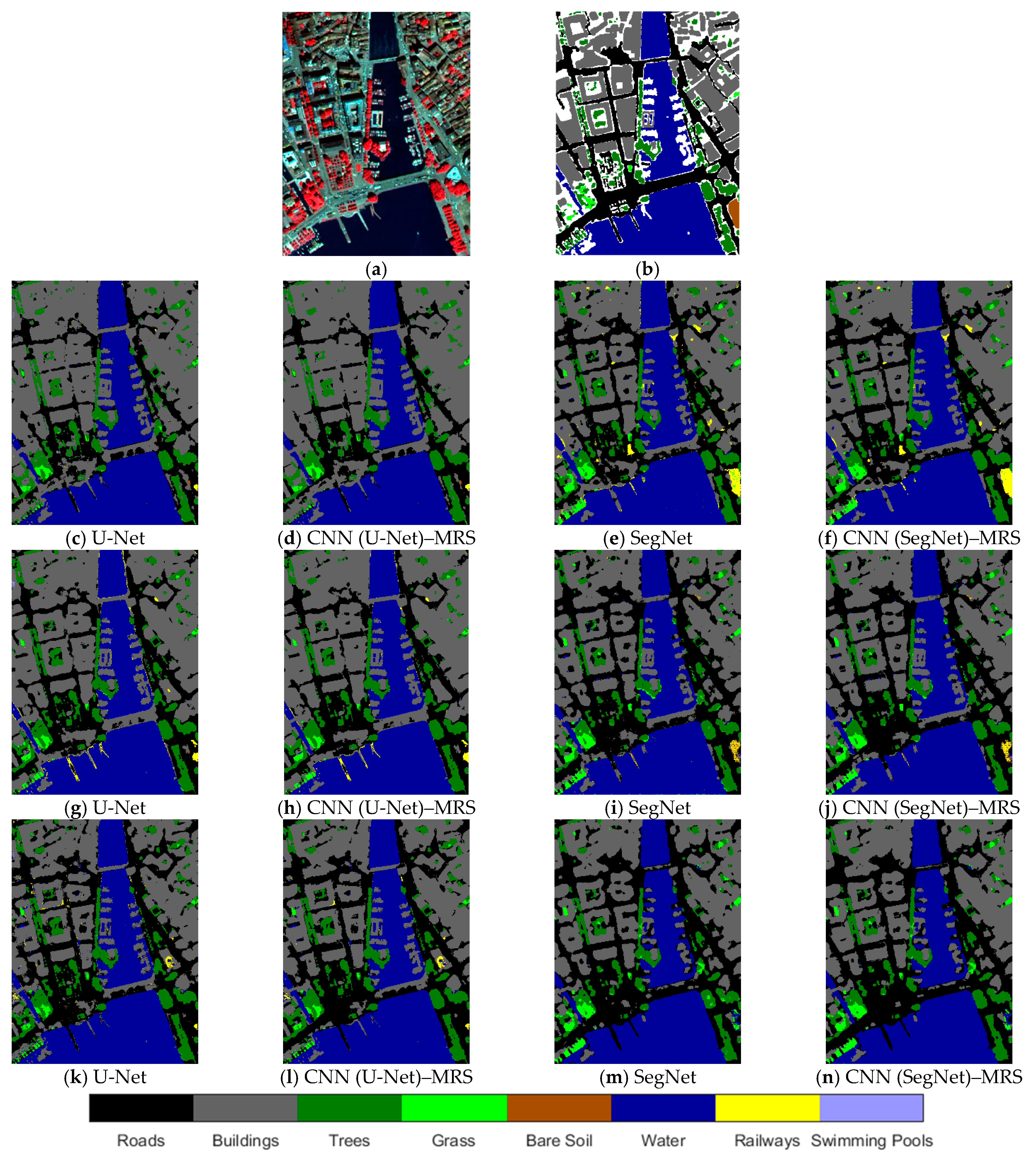
In the experiment, four bands were used. Like other studies in the literature, background was not considered in classification. In the CNN–MRS model, median filter size was 3 × 3. The ZH-16 and ZH-17 images were used as test images, and the ZH-20 image was used as validation data for the experiments. The proposed approach as CNN (SegNet)–MRS model had better performance on the public shared dataset than SegNet model in all metrics for the test images (Figure 18, Figure 19 and Table 15, Table 16). In CNN–MRS application, the object majority voting was applied as k = 80% for ZH-16 and ZH-17 images. Determining k threshold was dependent on the image, object size and category mixing. If there were more than k value segmentation predictions as classes in an object, then all the pixels were assigned the same class labeling of majority class, if not, first prediction class labels were preserved. Thus, the salt–pepper effect was decreased by applying the CNN–MRS model on the public VHR imagery dataset (Table 15).
Experiments on Zurich Summer dataset were compared with other state-of-the-art CNN models in the literature (Table 17). All methods were run on the same training, validation, and test data. The SegNet–MRS (128 × 128 patch) method in this study had the highest overall accuracy and weighted IoU in the ZH-16 test image, while it had the highest F1-score in the ZH-17 image.
6. Discussion
When considering the land cover map scale, the cartographic generalization would be helpful after applying the pixel-based deep learning approach. After applying CNN-based models, there is a salt and pepper effect when considering the scale as middle-scale reference thematic maps. LCCS has some generalization requirements, especially for too small objects. In the experiments in the Sentinel dataset, generally, ships and ports caused errors in the assessment. For instance, ships are accepted as water bodies in ground truth images as they are too small to accept as an object on that scale. In reference data, too small green areas, e.g., ships in the sea, were included in the neighboring wider area class (Figure 12 and Figure 13). This was a reason for the decrease in the class precision values (Figure 16) in the Sentinel dataset. In the Sentinel dataset, different dataset sizes were used in two test areas. The CNN (U-net)–MRS model was found to have a better classification with the five-band dataset, with overall accuracy of 97.31% and F1-score of 96.06% in Istanbul (Table 6). In the Kocaeli test area, the highest scores were found for the CNN (SegNet)–MRS model, with overall accuracy of 98.16% and F1-score of 92.54% for the seven-band dataset (Table 13).
Moreover, the CNN–MRS model is suitable for both the five- and seven-band datasets. For each experiment, it was revealed that the proposed CNN–MRS model has better results than the CNN-only models. As the noise ratio in the image increased in experiments, the amount of refinement in the classification increased using the CNN–MRS model (Figure 12, Figure 13, Figure 14 and Figure 15, Figure 18 and Figure 19). In addition, the McNemar test for the Sentinel dataset showed that comparing these different methodological models is significant (Table 14).
The Zurich Summer dataset used in the second experiment has very different weights of eight classes. Hence, as an imbalanced dataset, it affected the experimental results for LULC mapping. For this reason, swimming pools and bare land—the lowest weight classes in the datasets—could not be segmented in the CNN applications in the test images. This situation especially affected mean accuracy metric values (Table 15 and Table 16).
Previous studies of CNN for land cover mapping have generally focused on small areas. However, using traditional CNN methods in large areas produces coarser map results [21]. This study revealed that the classification results could be improved by combining object-based approaches and CNN models. Our findings are also consistent with similar studies [21,63].
7. Conclusions
In this study, we evaluated the effectiveness of the CNN–MRS model with combined mainstream and state-of-the-art CNN-based models for land cover mapping in two test areas situated in Turkey. The CNN–MRS methodology is also data-driven and can be adapted to different regional images of the same spatial resolution. The training and testing site sizes can be regularized according to DL model requirements. In the experiment, for this purpose, a test site area was chosen in a different city from the training site area. In addition, experiments were conducted with three different patch sizes for both CNN model classifiers. The CNN–MRS model and the other state-of-the-art CNN models were used for semantic segmentation for Sentinel and Zurich Summer datasets. The comparison results show the superiority of the CNN–MRS model using deep learning methods under different accuracy evaluation metrics.
Improving the producing and updating phase of regional EO tasks is a challenging task. The results of the proposed approach were compared with those of CNN-based state-of-the-art models. The proposed approach had a better classification ability than the CNN models in both Sentinel and public shared VHR imagery datasets. Related works in the literature considering the public dataset were also shown and discussed.
In EO missions, LULC mapping applications play a crucial role. Automatic classification systems and studies of refinement in map accuracies are tasks with great potential. For future studies, different band additions, including texture information and digital elevation model (DEM) layer, can also be applied. Additionally, we will focus on improving classification accuracy at larger patch sizes.
Author Contributions
Conceptualization, S.O.A., C.I.; Methodology, S.O.A.; Software, C.I.; Formal Analysis, S.O.A.; Investigation, S.O.A.; Resources, C.I.; Data Curation, S.O.A.; Writing—Original Draft Preparation, S.O.A.; Writing—Review & Editing, C.I.; Visualization, S.O.A.; Supervision, C.I. All authors have read and agreed to the published version of the manuscript.
Funding
This study was supported by Istanbul Technical University Scientific Research Office (BAP) with the project number MDK-2018-41541.
Institutional Review Board Statement
Not applicable.
Informed Consent Statement
Not applicable.
Data Availability Statement
Not applicable.
Conflicts of Interest
The authors declare no conflict of interest.
References
- Lee, S.-H.; Baik, J.-J. Evaluation of the vegetated urban canopy model (VUCM) and its impacts on urban boundary layer simulation. Asia Pac. J. Atmos. Sci. 2011, 47, 151–165. [Google Scholar] [CrossRef]
- Copernicus-CORINE Land Cover. Available online: https://land.copernicus.eu/pan-european/corine-land-cover (accessed on 25 December 2020).
- Loveland, T.; Merchant, J.; Brown, J.; Ohlen, D. Development of a land-cover characteristics database for the conterminous. Photogramm. Eng. Remote Sens. 1991, 57, 1453–1463. [Google Scholar]
- Brown, N.; Gerard, F.; Fuller, R. Mapping of land use classes within the CORINE land cover map of Great Britain. Cartogr. J. 2002, 39, 5–14. [Google Scholar] [CrossRef]
- Bronge, L.B.; Näslund-Landenmark, B. Wetland classification for Swedish CORINE Land Cover adopting a semi-automatic interactive approach. Can. J. Remote Sens. 2002, 28, 139–155. [Google Scholar] [CrossRef]
- Vali, A.; Comai, S.; Matteucci, M. Deep learning for land use and land cover classification based on hyperspectral and multi-spectral earth observation data: A review. Remote Sens. 2020, 12, 2495. [Google Scholar] [CrossRef]
- Pekkarinen, A.; Reithmaier, L.; Strobl, P. Pan-European forest/non-forest mapping with Landsat ETM+ and CORINE Land Cover 2000 data. ISPRS J. Photogramm. Remote Sens. 2009, 64, 171–183. [Google Scholar] [CrossRef]
- Heryadi, Y.; Miranda, E. Land Cover Classification Based on Sentinel-2 Satellite Imagery Using Convolutional Neural Network Model: A Case Study in Semarang Area, Indonesia. In Asian Conference on Intelligent Information and Database Systems; Springer: Cham, Switzerland, 2019; pp. 191–206. [Google Scholar]
- Qin, Y.; Wu, Y.; Li, B.; Gao, S.; Liu, M.; Zhan, Y. Semantic Segmentation of Building Roof in Dense Urban Environment with Deep Convolutional Neural Network: A Case Study Using GF2 VHR Imagery in China. Sensors 2019, 19, 1164. [Google Scholar] [CrossRef] [Green Version]
- Wurm, M.; Stark, T.; Zhu, X.X.; Weigand, M.; Taubenböck, H. Semantic segmentation of slums in satellite images using transfer learning on fully convolutional neural networks. ISPRS J. Photogramm. Remote Sens. 2019, 150, 59–69. [Google Scholar] [CrossRef]
- Neves, A.K.; Körting, T.S.; Fonseca, L.M.G.; Neto, C.D.G.; Wittich, D.; Costa, G.A.O.P.; Heipke, C. Semantic Segmentation of Brazilian Savanna Vegetation Using High Spatial Resolution Satellite Data and U-Net. ISPRS Ann. Photogramm. Remote Sens. Spat. Inf. Sci. 2020, 53, 505–511. [Google Scholar] [CrossRef]
- Yao, X.; Yang, H.; Wu, Y.; Wu, P.; Wang, B.; Zhou, X.; Wang, S. Land Use Classification of the Deep Convolutional Neural Network Method Reducing the Loss of Spatial Features. Sensors 2019, 19, 2792. [Google Scholar] [CrossRef] [Green Version]
- Demir, I.; Koperski, K.; Lindenbaum, D.; Pang, G.; Huang, J.; Basu, S.; Hughes, F.; Tuia, D.; Raskar, R. DeepGlobe 2018: A Challenge to Parse the Earth through Satellite Images. In Proceedings of the 2018 IEEE/CVF Conference on Computer Vision and Pattern Recognition Workshops, Salt Lake City, UT, USA, 18–22 June 2018; pp. 172–181. [Google Scholar]
- Sumbul, G.; Charfuelan, M.; Demir, B.; Markl, V. Bigearthnet: A Large-Scale Benchmark Archive for Remote Sensing Image Understanding. In Proceedings of the IGARSS 2019—2019 IEEE International Geoscience and Remote Sensing Symposium, Yokohama, Japan, 28 July–2 August 2019; pp. 5901–5904. [Google Scholar]
- Wang, S.; Chen, W.; Xie, S.M.; Azzari, G.; Lobell, D.B. Weakly Supervised Deep Learning for Segmentation of Remote Sensing Imagery. Remote Sens. 2020, 12, 207. [Google Scholar] [CrossRef] [Green Version]
- Audebert, N.; Le Saux, B.; Lefèvre, S. Semantic Segmentation of Earth Observation Data Using Multimodal and Multi-scale Deep Networks. In Asian Conference on Computer Vision; Springer: Berlin/Heidelberg, Germany, 2016; pp. 180–196. [Google Scholar]
- Kemker, R.; Salvaggio, C.; Kanan, C. Algorithms for semantic segmentation of multi-spectral remote sensing imagery using deep learning. ISPRS J. Photogramm. Remote Sens. 2018, 145, 60–77. [Google Scholar] [CrossRef] [Green Version]
- Liu, T.; Yang, L.; Lunga, D. Change detection using deep learning approach with object-based image analysis. Remote Sens. Environ. 2021, 256, 112308. [Google Scholar] [CrossRef]
- Ghorbanzadeh, O.; Tiede, D.; Wendt, L.; Sudmanns, M.; Lang, S. Transferable instance segmentation of dwellings in a refugee camp—Integrating CNN and OBIA. Eur. J. Remote Sens. 2021, 54, 127–140. [Google Scholar] [CrossRef]
- Papadomanolaki, M.; Vakalopoulou, M.; Karantzalos, K. A novel object-based deep learning framework for semantic seg-mentation of very high-resolution remote sensing data: Comparison with convolutional and fully convolutional networks. Remote Sens. 2019, 11, 684. [Google Scholar] [CrossRef] [Green Version]
- Martins, V.S.; Kaleita, A.L.; Gelder, B.K.; da Silveira, H.L.; Abe, C.A. Exploring multiscale object-based convolutional neural network (multi-OCNN) for remote sensing image classification at high spatial resolution. ISPRS J. Photogramm. Remote Sens. 2020, 168, 56–73. [Google Scholar] [CrossRef]
- Liu, T.; Abd-Elrahman, A.; Morton, J.; Wilhelm, V.L. Comparing fully convolutional networks, random forest, support vector machine, and patch-based deep convolutional neural networks for object-based wetland mapping using images from small unmanned aircraft system. GISci. Remote Sens. 2018, 55, 243–264. [Google Scholar] [CrossRef]
- Li, E.; Samat, A.; Liu, W.; Lin, C.; Bai, X. High-Resolution Imagery Classification Based on Different Levels of Information. Remote Sens. 2019, 11, 2916. [Google Scholar] [CrossRef] [Green Version]
- Tuia, D.; Volpi, M.; Moser, G. Decision Fusion with Multiple Spatial Supports by Conditional Random Fields. IEEE Trans. Geosci. Remote Sens. 2018, 56, 3277–3289. [Google Scholar] [CrossRef]
- Volpi, M.; Ferrari, V. Semantic segmentation of urban scenes by learning local class interactions. In Proceedings of the 2015 IEEE Conference on Computer Vision and Pattern Recognition Workshops, Boston, MA, USA, 7–12 June 2015; pp. 1–9. [Google Scholar]
- Goodfellow, I.; Bengio, Y.; Courville, A. Deep Learning; MIT Press: Cambridge, MA, USA, 2016. [Google Scholar]
- Badrinarayanan, V.; Kendall, A.; Cipolla, R. Segnet: A deep convolutional encoder-decoder architecture for image segmen-tation. IEEE Trans. Pattern Anal. Mach. Intell. 2017, 39, 2481–2495. [Google Scholar] [CrossRef]
- Abdollahi, A.; Pradhan, B.; Alamri, A.M. An ensemble architecture of deep convolutional Segnet and Unet networks for building semantic segmentation from high-resolution aerial images. Geocarto Int. 2020, 1–16. [Google Scholar] [CrossRef]
- Simonyan, K.; Zisserman, A. Very deep convolutional networks for large-scale image recognition. arXiv 2014, arXiv:1409.1556. [Google Scholar]
- Ronneberger, O.; Fischer, P.; Brox, T. U-net: Convolutional networks for biomedical image segmentation. In Proceedings of the International Conference on Medical Image Computing and Computer-Assisted Intervention, Cham, Switzerland, 5–9 October 2015; pp. 234–241. [Google Scholar]
- Baatz, M.; Schäpe, A. Multiresolution segmentation: An optimization approach for high quality multi-scale image segmen-tation. In Proceedings of the Angewandte Geographische Informations-Verarbeitung XII, Karlsruhe, Germany, 30 June 2000; Strobl, J., Blaschke, T., Griesebner, G., Eds.; Wichmann Verlag: Karlsruhe, Germany, 2000; pp. 12–23. [Google Scholar]
- Hossain, M.D.; Chen, D. Segmentation for Object-Based Image Analysis (OBIA): A review of algorithms and challenges from remote sensing perspective. ISPRS J. Photogramm. Remote Sens. 2019, 150, 115–134. [Google Scholar] [CrossRef]
- Wang, M. A multi-resolution remotely sensed image segmentation method combining rainfalling watershed algorithm and fast region merging. Int. Arch. Photogramm. Remote Sens. Spat. Inf. Sci. 2008, 37, 1213–1217. [Google Scholar]
- Tian, J.; Chen, D.-M. Optimization in multi-scale segmentation of high-resolution satellite images for artificial feature recognition. Int. J. Remote Sens. 2007, 28, 4625–4644. [Google Scholar] [CrossRef]
- Roni, R.; Jia, P. An Optimal Population Modeling Approach Using Geographically Weighted Regression Based on High-Resolution Remote Sensing Data: A Case Study in Dhaka City, Bangladesh. Remote Sens. 2020, 12, 1184. [Google Scholar] [CrossRef] [Green Version]
- Lang, S.; Hay, G.J.; Baraldi, A.; Tiede, D.; Blaschke, T. Geobia Achievements and Spatial Opportunities in the Era of Big Earth Observation Data. ISPRS Int. J. Geo-Inf. 2019, 8, 474. [Google Scholar] [CrossRef] [Green Version]
- Tetteh, G.; Gocht, A.; Schwieder, M.; Erasmi, S.; Conrad, C. Unsupervised Parameterization for Optimal Segmentation of Agricultural Parcels from Satellite Images in Different Agricultural Landscapes. Remote Sens. 2020, 12, 3096. [Google Scholar] [CrossRef]
- Wang, N.; Chen, F.; Yu, B.; Qin, Y. Segmentation of large-scale remotely sensed images on a Spark platform: A strategy for handling massive image tiles with the MapReduce model. ISPRS J. Photogramm. Remote Sens. 2020, 162, 137–147. [Google Scholar] [CrossRef]
- Ding, H.; Liu, K.; Chen, X.; Xiong, L.; Tang, G.; Qiu, F.; Strobl, J. Optimized Segmentation Based on the Weighted Aggregation Method for Loess Bank Gully Mapping. Remote Sens. 2020, 12, 793. [Google Scholar] [CrossRef] [Green Version]
- Kavzoglu, T.; Tonbul, H. An experimental comparison of multi-resolution segmentation, SLIC and K-means clustering for object-based classification of VHR imagery. Int. J. Remote Sens. 2018, 39, 6020–6036. [Google Scholar] [CrossRef]
- Rouse, J.W.; Haas, R.H.; Schell, J.A.; Deering, D.W. Monitoring Vegetation Systems in the Great Plains with ERTS; NASA Special Publication, 351; NASA: Washington, DC, USA, 1974; p. 309. [Google Scholar]
- Richardson, A.J.; Wiegand, C.L. Distinguishing vegetation from soil background information. Photogramm. Eng. Remote Sens. 1977, 43, 1541–1552. [Google Scholar]
- Pearson, R.L.; Miller, L.D. Remote mapping of standing crop biomass for estimation of the productivity of the shortgrass prairie. Remote Sens. Environ. 1972, VIII, 1355. [Google Scholar]
- Tucker, C.J. Red and photographic infrared linear combinations for monitoring vegetation. Remote Sens. Environ. 1979, 8, 127–150. [Google Scholar] [CrossRef] [Green Version]
- Alpaydın, E. Introduction to Machine Learning, 2nd ed.; MIT Press: London, UK, 2010. [Google Scholar]
- Congalton, R.G. A review of assessing the accuracy of classifications of remotely sensed data. Remote Sens. Environ. 1991, 37, 35–46. [Google Scholar] [CrossRef]
- Cohen, J. A Coefficient of Agreement for Nominal Scales. Educ. Psychol. Meas. 1960, 20, 37–46. [Google Scholar] [CrossRef]
- Chatziantoniou, A.; Psomiadis, E.; Petropoulos, G.P. Co-Orbital Sentinel 1 and 2 for LULC mapping with emphasis on wet-lands in a mediterranean setting based on machine learning. Remote Sens. 2017, 9, 1259. [Google Scholar] [CrossRef] [Green Version]
- Powers, D.M. Evaluation: From precision, recall and F-measure to ROC, informedness, markedness and correlation. Int. J. Mach. Learn. Technol. 2011, 2, 37–63. [Google Scholar]
- McNemar, Q. Note on the sampling error of the difference between correlated proportions or percentages. Psychometrika 1947, 12, 153–157. [Google Scholar] [CrossRef]
- Foody, G.M. Thematic map comparison: Evaluating the statistical significance of differences in classification accuracy. Photogramm. Eng. Remote Sens. 2004, 70, 627633. [Google Scholar] [CrossRef]
- Li, H.; Wang, C.; Zhong, C.; Zhang, Z.; Liu, Q. Mapping Typical Urban LULC from Landsat Imagery without Training Samples or Self-Defined Parameters. Remote Sens. 2017, 9, 700. [Google Scholar] [CrossRef] [Green Version]
- Hütt, C.; Koppe, W.; Miao, Y.; Bareth, G. Best Accuracy Land Use/Land Cover (LULC) Classification to Derive Crop Types Using Multitemporal, Multisensor, and Multi-Polarization SAR Satellite Images. Remote Sens. 2016, 8, 684. [Google Scholar] [CrossRef] [Green Version]
- Quan, Y.; Tong, Y.; Feng, W.; Dauphin, G.; Huang, W.; Xing, M. A Novel Image Fusion Method of Multi-Spectral and SAR Images for Land Cover Classification. Remote Sens. 2020, 12, 3801. [Google Scholar] [CrossRef]
- Clinton, N.; Holt, A.; Scarborough, J.; Yan, L.; Gong, P. Accuracy Assessment Measures for Object-based Image Segmentation Goodness. Photogramm. Eng. Remote Sens. 2010, 76, 289–299. [Google Scholar] [CrossRef]
- Kavzoglu, T.; Tonbul, H. A comparative study of segmentation quality for multi-resolution segmentation and watershed transform. In Proceedings of the 2017 8th International Conference on Recent Advances in Space Technologies (RAST), Istanbul, Turkey, 19–22 June 2017; pp. 113–117. [Google Scholar]
- Lucieer, A.; Stein, A. Existential uncertainty of spatial objects segmented from satellite sensor imagery. IEEE Trans. Geosci. Remote Sens. 2002, 40, 2518–2521. [Google Scholar] [CrossRef] [Green Version]
- Winter, S. Location similarity of regions. ISPRS J. Photogramm. Remote Sens. 2000, 55, 189–200. [Google Scholar] [CrossRef]
- Edwards, A.L. Note on the “correction for continuity” in testing the significance of the difference between correlated proportions. Psychometrika 1948, 13, 185–187. [Google Scholar] [CrossRef]
- Long, J.; Shelhamer, E.; Darrell, T. Fully convolutional networks for semantic segmentation. In Proceedings of the IEEE Conference on Computer Vision and Pattern Recognition, Boston, MA, USA, 7–12 June 2015; pp. 3431–3440. [Google Scholar]
- Chen, L.C.; Papandreou, G.; Schroff, F.; Adam, H. Rethinking atrous convolution for semantic image segmentation. arXiv 2017, arXiv:1706.05587. [Google Scholar]
- Chen, L.C.; Zhu, Y.; Papandreou, G.; Schroff, F.; Adam, H. Encoder-decoder with atrous separable convolution for semantic image segmentation. In Proceedings of the European Conference on Computer Vision (ECCV), Munich, Germany, 8–14 September 2018; pp. 801–818. [Google Scholar]
- Du, S.; Du, S.; Liu, B.; Zhang, X. Incorporating DeepLabv3+ and object-based image analysis for semantic segmentation of very high resolution remote sensing images. Int. J. Digit. Earth 2020, 14, 1–22. [Google Scholar] [CrossRef]
Figure 1.
Distribution of selected cities for study area in Turkey.

Figure 2.
Subset images of Sentinel-2A in Istanbul city for the experiment.

Figure 3.
Selected test image of Sentinel-2A in Kocaeli city for the experiment.

Figure 4.
Subset image of Sentinel-2A for the training area 4 in Mugla city for the experiment in Mugla city.
Figure 4.
Subset image of Sentinel-2A for the training area 4 in Mugla city for the experiment in Mugla city.

Figure 5.
Sample image of Zurich Summer dataset (ZH-12): (a) original image; (b) ground truth.

Figure 6.
Flowchart of the study.

Figure 7.
An illustration of the SegNet architecture of our study [27].
Figure 7.
An illustration of the SegNet architecture of our study [27].

Figure 8.
An illustration of the U-Net architecture of our study.

Figure 9.
Schematic explanation of majority voting within segmentation.

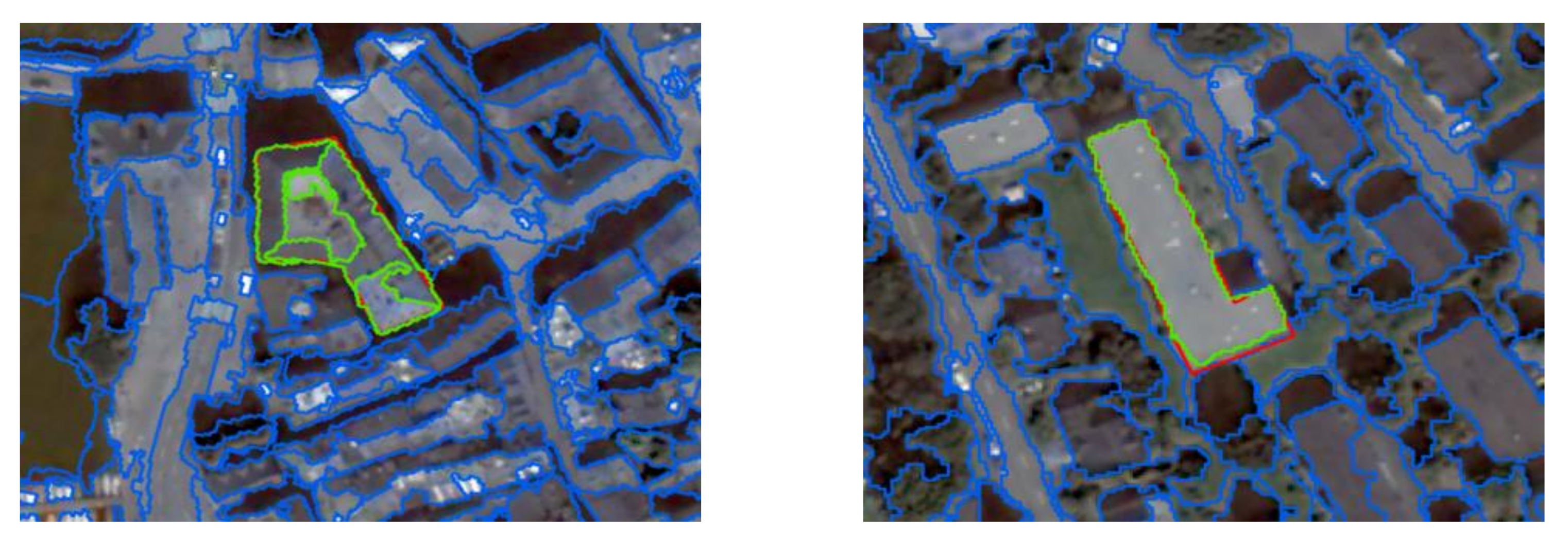
Figure 10.
Samples of segmentation from Sentinel dataset. Red line refers to reference object; green line refers to MRS segments.
Figure 10.
Samples of segmentation from Sentinel dataset. Red line refers to reference object; green line refers to MRS segments.

Figure 11.
Samples of segmentation from Zurich Summer dataset. Red line refers to reference object; green line refers to MRS segments.
Figure 11.
Samples of segmentation from Zurich Summer dataset. Red line refers to reference object; green line refers to MRS segments.

Figure 12.
Istanbul test area results of CNN models and CNN–MRS models with 5-band dataset (c–f): 32 × 32 patch size; (g–j): 64 × 64 patch size; (k–n): 128 × 128 patch size.
Figure 12.
Istanbul test area results of CNN models and CNN–MRS models with 5-band dataset (c–f): 32 × 32 patch size; (g–j): 64 × 64 patch size; (k–n): 128 × 128 patch size.

Figure 13.
Istanbul test area results of CNN models and CNN–MRS models with 7-band dataset (c–f): 32 × 32 patch size; (g–j): 64 × 64 patch size; (k–n): 128 × 128 patch size.
Figure 13.
Istanbul test area results of CNN models and CNN–MRS models with 7-band dataset (c–f): 32 × 32 patch size; (g–j): 64 × 64 patch size; (k–n): 128 × 128 patch size.

Figure 14.
Kocaeli test area results of CNN models and CNN–MRS models with five-band dataset (c–f): 32 × 32 patch size; (g–j): 64 × 64 patch size; (k–n): 128 × 128 patch size.
Figure 14.
Kocaeli test area results of CNN models and CNN–MRS models with five-band dataset (c–f): 32 × 32 patch size; (g–j): 64 × 64 patch size; (k–n): 128 × 128 patch size.

Figure 15.
Kocaeli test area results of CNN models and CNN–MRS models with 7-band dataset (c–f): 32 × 32 patch size; (g–j): 64 × 64 patch size; (k–n): 128 × 128 patch size).
Figure 15.
Kocaeli test area results of CNN models and CNN–MRS models with 7-band dataset (c–f): 32 × 32 patch size; (g–j): 64 × 64 patch size; (k–n): 128 × 128 patch size).

Figure 16.
Precision and recall values of different patch sizes for Istanbul test area. Pro.U is proposed approach as CNN (U-Net)–MRS and Pro.S. is proposed approach as CNN (SegNet)–MRS.
Figure 16.
Precision and recall values of different patch sizes for Istanbul test area. Pro.U is proposed approach as CNN (U-Net)–MRS and Pro.S. is proposed approach as CNN (SegNet)–MRS.

Figure 17.
Precision and recall values of different patch sizes for Kocaeli test area. Pro.U is proposed approach as CNN (U-Net)–MRS and Pro.S is proposed approach as CNN (SegNet)–MRS.
Figure 17.
Precision and recall values of different patch sizes for Kocaeli test area. Pro.U is proposed approach as CNN (U-Net)–MRS and Pro.S is proposed approach as CNN (SegNet)–MRS.

Figure 18.
Results of Zurich dataset (ZH-16): (a) original image; (b) ground truth; (c–f) 32 × 32 patch size; (g–j) 64 × 64 patch size; (k–n) 128 × 128 patch size.
Figure 18.
Results of Zurich dataset (ZH-16): (a) original image; (b) ground truth; (c–f) 32 × 32 patch size; (g–j) 64 × 64 patch size; (k–n) 128 × 128 patch size.

Figure 19.
Results of Zurich dataset (ZH-17): (a) original image; (b) ground truth; (c–f) 32 × 32 patch size; (g–j) 64 × 64 patch size; (k–n) 128 × 128 patch size.
Figure 19.
Results of Zurich dataset (ZH-17): (a) original image; (b) ground truth; (c–f) 32 × 32 patch size; (g–j) 64 × 64 patch size; (k–n) 128 × 128 patch size.


Table 1.
Training data class distribution for Sentinel dataset.
| Class | Pixel Count | Percentage (%) |
|---|---|---|
| Artificial surfaces | 1,972,691 | 30.0 |
| Forest and semi-natural areas | 2,266,083 | 34.5 |
| Water bodies | 2,331,916 | 35.5 |
Table 2.
Multispectral indices used in this study.
| Spectral Index | Formula | Authors |
|---|---|---|
| NDVI | Rouse, Haas, Schell, and Deering (1974) [41] | |
| DVI | Richardson and Wiegand (1992) [42] | |
| SR | Pearson and Miller (1972) [43] |
Table 3.
Contingency matrix between two models.
| Model 1 | Model 2 | ||
|---|---|---|---|
| Correct | Incorrect | ||
| Model 1 | Correct | f11 | f12 |
| Model 2 | Incorrect | f21 | f22 |
Table 4.
Segmentation quality metrics for Sentinel test dataset.
| OS | US | RMSE | AFI | QR | |
|---|---|---|---|---|---|
| Test Image (Istanbul) | 0.056 | 0.020 | 0.042 | 0.037 | 0.926 |
| Test Image (Kocaeli) | 0.030 | 0.041 | 0.036 | −0.012 | 0.931 |
Table 5.
Segmentation quality metrics for Zurich Summer dataset.
| OS | US | RMSE | AFI | QR | |
|---|---|---|---|---|---|
| Test Image (Image-16) | 0.071 | 0.021 | 0.053 | 0.051 | 0.910 |
| Test Image (Image-17) | 0.085 | 0.015 | 0.061 | 0.071 | 0.881 |
Table 6.
Istanbul test site with 5 bands: performance metrics with U-Net.
| Land Cover | U-Net Model | CNN (U-Net)–MRS | ||||||||||
|---|---|---|---|---|---|---|---|---|---|---|---|---|
| 32 × 32 | 64 × 64 | 128 × 128 | 32 × 32 | 64 × 64 | 128 × 128 | |||||||
| F1% | IoU% | F1% | IoU% | F1% | IoU% | F1% | IoU% | F1% | IoU% | F1% | IoU% | |
| AR | 75.57 | 86.39 | 90.45 | 90.63 | 71.99 | 84.67 | 94.73 | 95.00 | 95.22 | 96.02 | 90.46 | 92.52 |
| FSN | 78.03 | 66.58 | 86.19 | 77.41 | 73.39 | 60.28 | 93.70 | 86.34 | 94.52 | 89.43 | 88.69 | 79.15 |
| WB | 75.54 | 93.42 | 93.82 | 93.51 | 75.19 | 93.81 | 98.34 | 99.51 | 98.43 | 99.31 | 97.58 | 99.25 |
| OA | 90.16 | 93.39 | 88.65 | 96.59 | 97.31 | 94.78 | ||||||
| Av. F1 | 76.38 | 90.15 | 73.52 | 95.59 | 96.06 | 92.24 | ||||||
| Kappa | 80.40 | 86.85 | 76.87 | 93.16 | 94.66 | 89.38 | ||||||
Table 7.
Istanbul test site with 5 bands: performance metrics with SegNet.
| Land Cover | SegNet Model | CNN (SegNet)–MRS | ||||||||||
|---|---|---|---|---|---|---|---|---|---|---|---|---|
| 32 × 32 | 64 × 64 | 128 × 128 | 32 × 32 | 64 × 64 | 128 × 128 | |||||||
| F1 % | IoU% | F1% | IoU% | F1% | IoU% | F1 % | IoU% | F1% | IoU% | F1% | IoU% | |
| AR | 71.14 | 82.16 | 83.21 | 86.79 | 43.73 | 70.60 | 86.64 | 92.19 | 90.19 | 93.64 | 59.11 | 79.37 |
| FSN | 70.89 | 54.77 | 84.56 | 72.67 | 51.36 | 53.67 | 82.74 | 79.38 | 89.76 | 85.33 | 60.46 | 65.12 |
| WB | 65.35 | 76.46 | 61.15 | 84.82 | 72.79 | 83.46 | 87.01 | 90.75 | 80.69 | 96.09 | 92.35 | 93.46 |
| OA | 85.71 | 90.56 | 79.41 | 94.09 | 95.70 | 86.43 | ||||||
| Av. F1 | 69.13 | 76.31 | 55.96 | 85.46 | 86.88 | 70.64 | ||||||
| Kappa | 69.98 | 81.97 | 64.73 | 88.18 | 91.66 | 75.95 | ||||||
Table 8.
Istanbul test site with 7 bands: performance metrics with U-Net.
| Land Cover | U-Net Model | CNN (U-Net)–MRS | |||||||||||
|---|---|---|---|---|---|---|---|---|---|---|---|---|---|
| 32 × 32 | 64 × 64 | 128 × 128 | 32 × 32 | 64 × 64 | 128 × 128 | ||||||||
| F1 % | IoU% | F1% | IoU% | F1% | IoU% | F1 % | IoU% | F1% | IoU% | F1% | IoU% | ||
| AR | 89.12 | 89.53 | 88.27 | 89.12 | 61.83 | 78.66 | 93.34 | 94.70 | 90.82 | 93.66 | 89.71 | 93.19 | |
| FSN | 84.84 | 74.53 | 80.91 | 71.61 | 70.40 | 61.19 | 92.47 | 85.81 | 88.63 | 82.18 | 88.45 | 84.80 | |
| WB | 94.07 | 90.77 | 94.54 | 92.91 | 78.53 | 92.05 | 98.22 | 97.79 | 98.48 | 98.93 | 96.68 | 98.93 | |
| OA | 92.48 | 92.05 | 85.38 | 96.31 | 95.55 | 95.57 | |||||||
| Av. F1 | 89.34 | 87.91 | 70.25 | 94.68 | 92.64 | 91.61 | |||||||
| Kappa | 84.76 | 83.81 | 73.36 | 92.59 | 91.00 | 91.55 | |||||||
Table 9.
Istanbul test site with 7 bands: performance metrics with SegNet.
| Land Cover | SegNet Model | CNN (SegNet)–MRS | ||||||||||
|---|---|---|---|---|---|---|---|---|---|---|---|---|
| 32 × 32 | 64 × 64 | 128 × 128 | 32 × 32 | 64 × 64 | 128 × 128 | |||||||
| F1% | IoU% | F1% | IoU% | F1% | IoU% | F1% | IoU% | F1% | IoU% | F1% | IoU% | |
| AR | 74.74 | 84.23 | 89.89 | 89.67 | 84.07 | 88.03 | 85.81 | 91.75 | 93.05 | 95.03 | 92.57 | 95.56 |
| FSN | 74.93 | 70.45 | 90.12 | 75.07 | 83.81 | 74.44 | 84.86 | 82.41 | 91.67 | 86.95 | 93.37 | 89.79 |
| WB | 65.55 | 87.77 | 81.02 | 89.88 | 69.23 | 90.06 | 84.42 | 97.49 | 98.57 | 98.02 | 94.08 | 98.33 |
| OA | 89.23 | 92.49 | 91.60 | 94.60 | 96.57 | 97.09 | ||||||
| Av. F1 | 71.74 | 87.01 | 79.04 | 85.03 | 94.43 | 93.34 | ||||||
| Kappa | 80.12 | 84.99 | 84.03 | 89.80 | 93.17 | 94.40 | ||||||
Table 10.
Kocaeli test site with 5 bands: performance metrics with U-Net.
| Land Cover | U-Net Model | CNN (U-Net)–MRS | ||||||||||
|---|---|---|---|---|---|---|---|---|---|---|---|---|
| 32 × 32 | 64 × 64 | 128 × 128 | 32 × 32 | 64 × 64 | 128 × 128 | |||||||
| F1 % | IoU% | F1% | IoU% | F1% | IoU% | F1 % | IoU% | F1% | IoU% | F1% | IoU% | |
| AR | 73.72 | 83.74 | 87.73 | 88.21 | 67.59 | 80.49 | 93.81 | 95.35 | 91.76 | 94.27 | 86.51 | 92.73 |
| FSN | 66.07 | 76.05 | 73.47 | 85.05 | 59.31 | 69.94 | 88.87 | 92.80 | 88.42 | 92.01 | 81.18 | 88.41 |
| WB | 87.33 | 98.48 | 95.56 | 97.75 | 86.67 | 98.73 | 97.63 | 99.40 | 98.98 | 99.36 | 97.43 | 99.48 |
| OA | 94.43 | 96.01 | 93.22 | 98.44 | 98.17 | 97.60 | ||||||
| Av. F1 | 75.71 | 85.59 | 71.19 | 93.42 | 96.46 | 88.37 | ||||||
| Kappa | 90.88 | 93.50 | 88.86 | 97.44 | 97.01 | 96.07 | ||||||
Table 11.
Kocaeli test site with 5 bands: performance metrics with SegNet.
| Land Cover | SegNet Model | CNN (SegNet)–MRS | ||||||||||||
|---|---|---|---|---|---|---|---|---|---|---|---|---|---|---|
| 32 × 32 | 64 × 64 | 128 × 128 | 32 × 32 | 64 × 64 | 128 × 128 | |||||||||
| F1 % | IoU% | F1% | IoU% | F1% | IoU% | F1 % | IoU% | F1% | IoU% | F1% | IoU% | |||
| AR | 52.00 | 73.85 | 84.46 | 84.78 | 59.27 | 72.65 | 83.28 | 88.41 | 88.06 | 91.31 | 72.70 | 80.45 | ||
| FSN | 47.56 | 62.88 | 75.84 | 80.97 | 53.23 | 67.73 | 80.07 | 88.33 | 84.47 | 89.54 | 60.39 | 78.11 | ||
| WB | 74.52 | 94.69 | 76.71 | 96.67 | 70.52 | 95.76 | 91.44 | 97.26 | 89.62 | 98.54 | 89.93 | 97.99 | ||
| OA | 89.85 | 94.72 | 90.48 | 96.27 | 97.24 | 93.94 | ||||||||
| Av. F1 | 58.03 | 79.00 | 61.01 | 84.93 | 87.38 | 74.34 | ||||||||
| Kappa | 83.43 | 91.79 | 84.57 | 93.93 | 95.48 | 90.16 | ||||||||
Table 12.
Kocaeli test site with 7 bands: performance metrics with U-Net.
| Land Cover | U-Net Model | CNN (U-Net)–MRS | ||||||||||||
|---|---|---|---|---|---|---|---|---|---|---|---|---|---|---|
| 32 × 32 | 64 × 64 | 128 × 128 | 32 × 32 | 64 × 64 | 128 × 128 | |||||||||
| F1 % | IoU% | F1% | IoU% | F1% | IoU% | F1 % | IoU% | F1% | IoU% | F1% | IoU% | |||
| AR | 82.74 | 84.99 | 70.06 | 82.92 | 66.71 | 76.76 | 88.64 | 91.89 | 85.27 | 91.30 | 89.76 | 89.39 | ||
| FSN | 74.80 | 85.85 | 68.62 | 83.17 | 62.74 | 71.41 | 89.72 | 93.31 | 81.69 | 91.34 | 76.51 | 85.60 | ||
| WB | 86.48 | 95.53 | 59.34 | 94.55 | 92.66 | 98.13 | 93.85 | 97.49 | 93.04 | 97.56 | 98.38 | 99.44 | ||
| OA | 94.92 | 93.98 | 92.36 | 97.42 | 97.14 | 96.70 | ||||||||
| Av. F1 | 81.34 | 66.01 | 74.04 | 90.74 | 86.67 | 88.22 | ||||||||
| Kappa | 91.77 | 90.23 | 87.62 | 95.81 | 95.35 | 94.62 | ||||||||
Table 13.
Kocaeli test site with 7 bands: performance metrics with SegNet.
| Land Cover | SegNet Model | CNN (SegNet)–MRS | ||||||||||||
|---|---|---|---|---|---|---|---|---|---|---|---|---|---|---|
| 32 × 32 | 64 × 64 | 128 × 128 | 32 × 32 | 64 × 64 | 128 × 128 | |||||||||
| F1 % | IoU% | F1% | IoU% | F1% | IoU% | F1 % | IoU% | F1% | IoU% | F1% | IoU% | |||
| AR | 80.10 | 81.82 | 90.37 | 88.68 | 83.94 | 85.05 | 87.77 | 88.76 | 92.50 | 94.37 | 90.26 | 92.29 | ||
| FSN | 59.14 | 77.78 | 85.53 | 86.24 | 79.72 | 83.31 | 83.83 | 86.37 | 88.94 | 92.07 | 87.64 | 90.92 | ||
| WB | 44.97 | 96.39 | 91.34 | 97.92 | 76.46 | 97.44 | 94.07 | 99.06 | 96.19 | 99.20 | 90.34 | 98.84 | ||
| OA | 93.67 | 96.29 | 95.25 | 96.60 | 98.16 | 97.62 | ||||||||
| Av. F1 | 61.40 | 89.08 | 80.04 | 88.56 | 92.54 | 89.41 | ||||||||
| Kappa | 89.73 | 93.93 | 92.22 | 94.46 | 96.98 | 96.11 | ||||||||
Table 14.
McNemar test results for models.
| Test Area | Methods | 5-Band | 7-Band | ||||
|---|---|---|---|---|---|---|---|
| 32 × 32 | 64 × 64 | 128 × 128 | 32 × 32 | 64 × 64x | 128 × 128 | ||
| Istanbul | U-Net and CNN (U-Net)–MRS | 40,962.9 | 23,308.6 | 36,789.4 | 25,864.9 | 23,417.3 | 64,731.2 |
| SegNet and CNN (SegNet)–MRS | 54,857.5 | 36,063.2 | 46,511.0 | 38,202.1 | 28,055.5 | 39,722.9 | |
| Kocaeli | U-Net and CNN (U-Net)–MRS | 26,810.9 | 14,914.7 | 28,721.9 | 15,360.0 | 19,305.0 | 25,002.5 |
| SegNet and CNN (SegNet)–MRS | 43,818.4 | 17,189.7 | 22,612.7 | 19,273.0 | 13,006.4 | 14,391.3 |
Table 15.
Experimental results for ZH 16 image of the Zurich Summer dataset.
| Method | OA % | F1-Score % | Mean Acc. % | Weighted IoU% |
|---|---|---|---|---|
| 32 × 32 patch size | ||||
| SegNet | 88.76 | 81.05 | 71.13 | 81.41 |
| U-Net | 85.49 | 74.04 | 66.08 | 75.57 |
| SegNet–MRS * | 89.73 | 84.17 | 71.71 | 82.76 |
| U-Net–MRS * | 85.98 | 76.04 | 66.73 | 76.20 |
| 64 × 64 patch size | ||||
| SegNet | 90.05 | 74.92 | 75.54 | 82.88 |
| U-Net | 87.88 | 73.66 | 68.56 | 79.44 |
| SegNet–MRS * | 90.91 | 77.29 | 75.87 | 84.15 |
| U-Net–MRS * | 88.32 | 72.36 | 68.45 | 79.95 |
| 128 × 128 patch size | ||||
| SegNet | 91.09 | 72.17 | 72.93 | 84.39 |
| U-Net | 89.80 | 69.22 | 68.22 | 82.48 |
| SegNet–MRS * | 92.03 | 72.79 | 73.41 | 85.88 |
| U-Net–MRS * | 91.04 | 69.05 | 68.94 | 84.29 |
* Implementation of the proposed approach.
Table 16.
Experimental results for ZH 17 image of the Zurich Summer dataset.
| Method | OA % | F1-Score % | Mean Acc. % | Weighted IoU% |
|---|---|---|---|---|
| 32 × 32 patch size | ||||
| SegNet | 88.48 | 90.92 | 62.88 | 79.73 |
| U-Net | 85.83 | 68.72 | 65.51 | 78.82 |
| SegNet–MRS * | 89.17 | 91.53 | 62.88 | 80.88 |
| U-net–MRS * | 86.40 | 69.45 | 65.93 | 75.72 |
| 64 × 64 patch size | ||||
| SegNet | 90.31 | 75.68 | 59.51 | 82.42 |
| U-Net | 87.65 | 87.25 | 73.20 | 77.98 |
| SegNet–MRS * | 90.67 | 75.78 | 59.56 | 83.00 |
| U-Net–MRS * | 88.19 | 86.33 | 73.62 | 78.90 |
| 128 × 128 patch size | ||||
| SegNet | 89.48 | 87.93 | 58.58 | 80.78 |
| U-Net | 85.77 | 84.35 | 72.17 | 75.48 |
| SegNet–MRS * | 89.94 | 87.76 | 58.43 | 81.52 |
| U-Net–MRS * | 86.33 | 84.66 | 71.80 | 76.40 |
* Implementation of the proposed approach.
Table 17.
Comparison with other approaches on Zurich Summer dataset (The values are given as %).
| ZH-16 Image | ZH-17 Image | |||||
|---|---|---|---|---|---|---|
| Method | OA | F1-Score | Weighted IoU | OA | F1-Score | Weighted IoU |
| FCN [60] | 81.02 | 66.13 | 69.92 | 77.14 | 67.42 | 62.81 |
| DeeplabV3 + ResNet50 [61] | 88.02 | 69.54 | 79.38 | 89.21 | 81.36 | 80.74 |
| DeeplabV3 + Xception [62] | 90.29 | 76.02 | 83.05 | 90.21 | 82.11 | 82.33 |
| CNN–MRS * | 92.03 | 72.79 | 85.88 | 89.94 | 87.76 | 81.52 |
* Our implementation of the proposed methodology.
Publisher’s Note: MDPI stays neutral with regard to jurisdictional claims in published maps and institutional affiliations. |
© 2021 by the authors. Licensee MDPI, Basel, Switzerland. This article is an open access article distributed under the terms and conditions of the Creative Commons Attribution (CC BY) license (https://creativecommons.org/licenses/by/4.0/).
Share and Cite
MDPI and ACS Style
Atik, S.O.; Ipbuker, C. Integrating Convolutional Neural Network and Multiresolution Segmentation for Land Cover and Land Use Mapping Using Satellite Imagery. Appl. Sci. 2021, 11, 5551. https://doi.org/10.3390/app11125551
AMA Style
Atik SO, Ipbuker C. Integrating Convolutional Neural Network and Multiresolution Segmentation for Land Cover and Land Use Mapping Using Satellite Imagery. Applied Sciences. 2021; 11(12):5551. https://doi.org/10.3390/app11125551
Chicago/Turabian StyleAtik, Saziye Ozge, and Cengizhan Ipbuker. 2021. "Integrating Convolutional Neural Network and Multiresolution Segmentation for Land Cover and Land Use Mapping Using Satellite Imagery" Applied Sciences 11, no. 12: 5551. https://doi.org/10.3390/app11125551
Note that from the first issue of 2016, this journal uses article numbers instead of page numbers. See further details here.