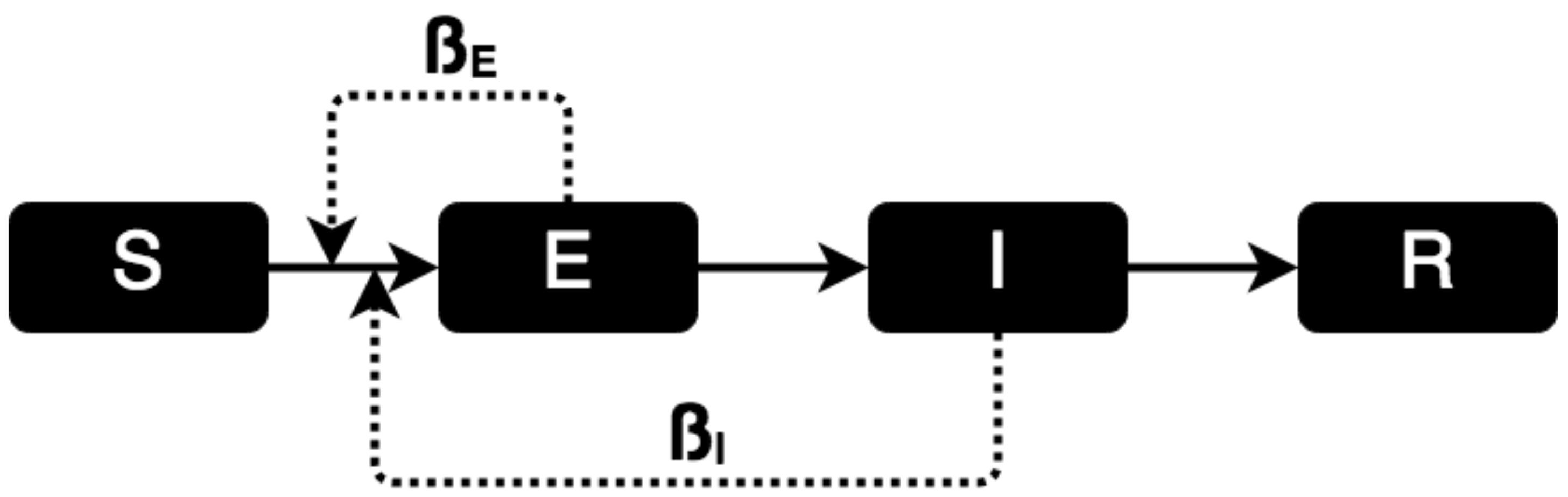
Figure 1.
Scheme of the SIR Model.
Figure 1.
Scheme of the SIR Model.
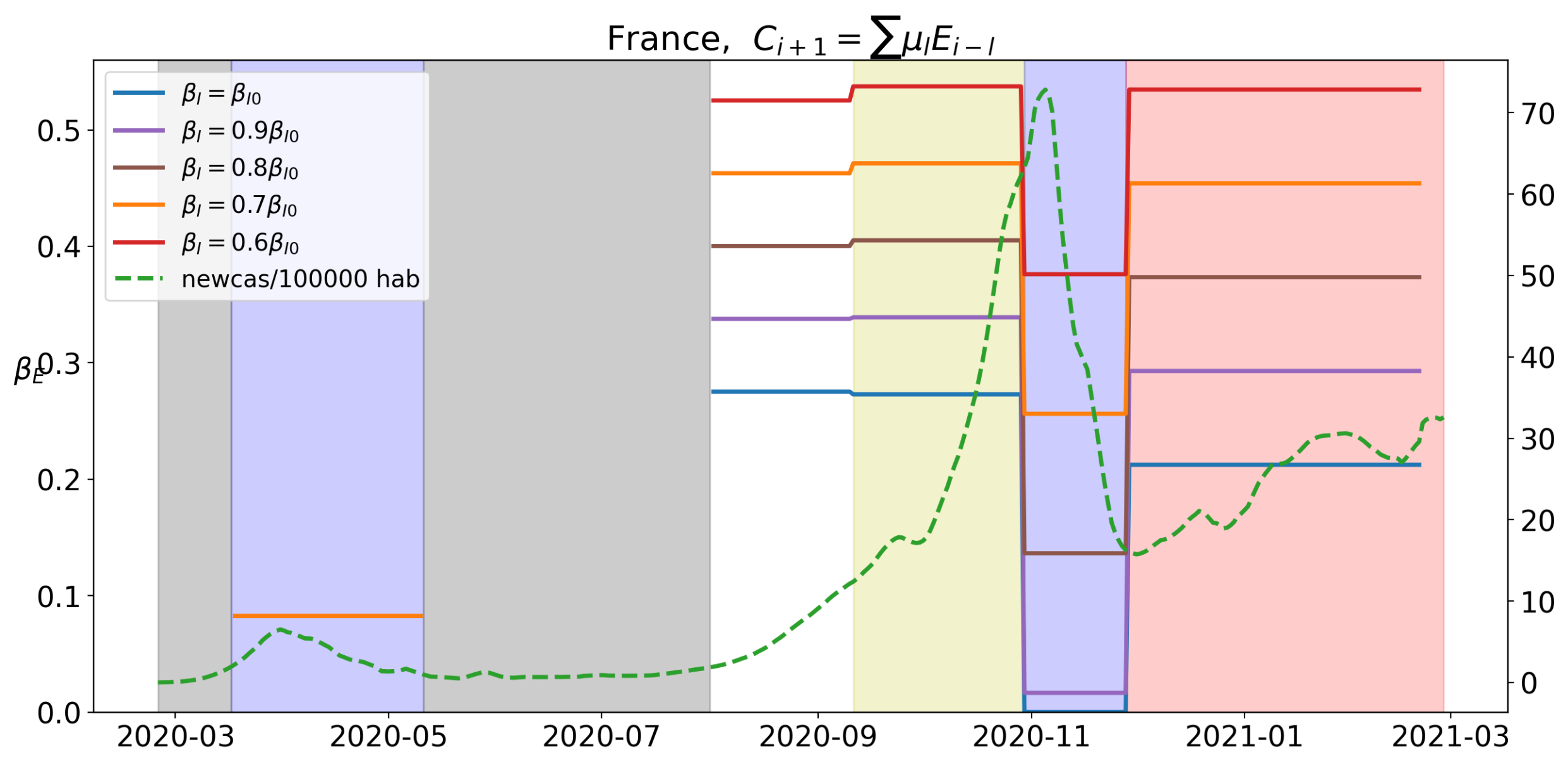
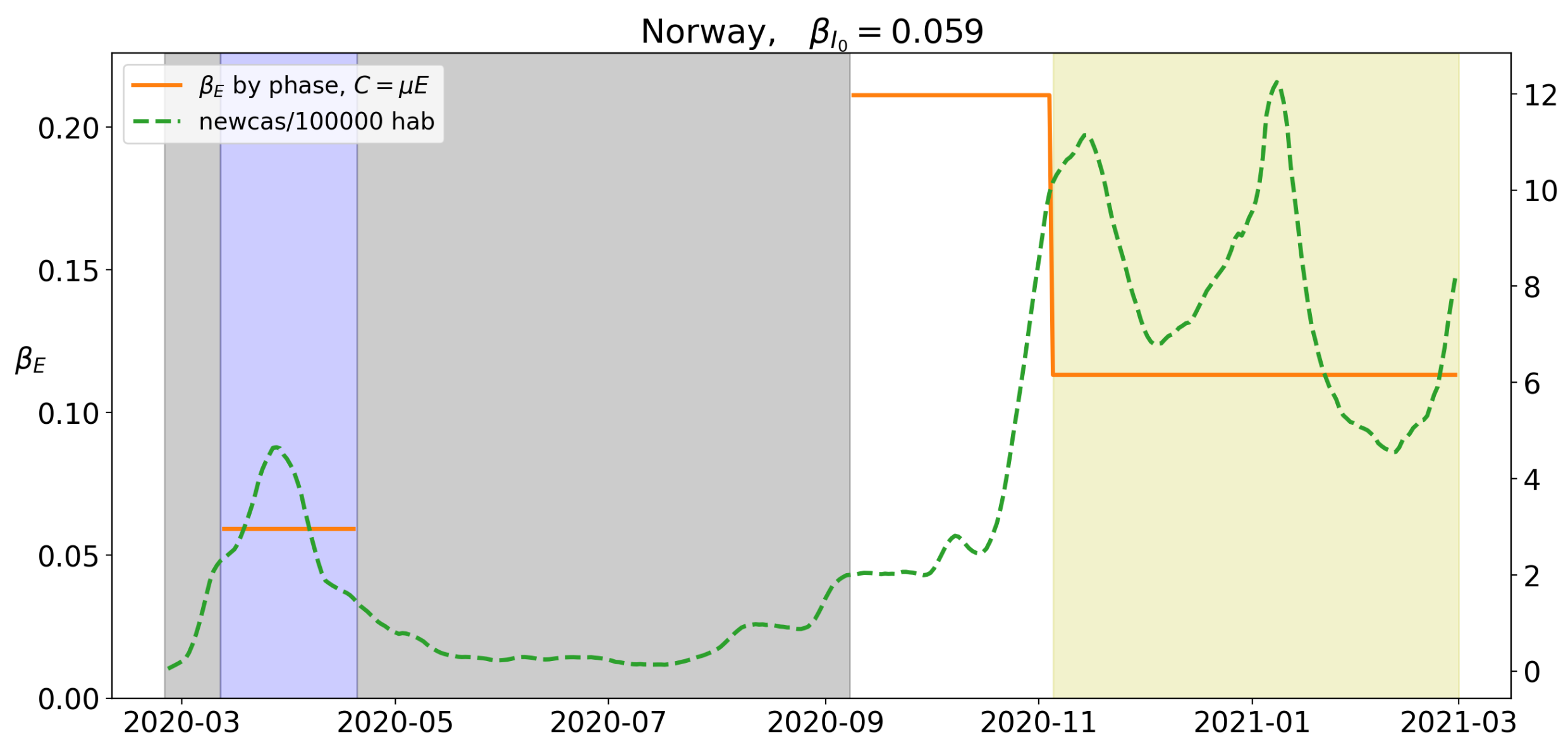
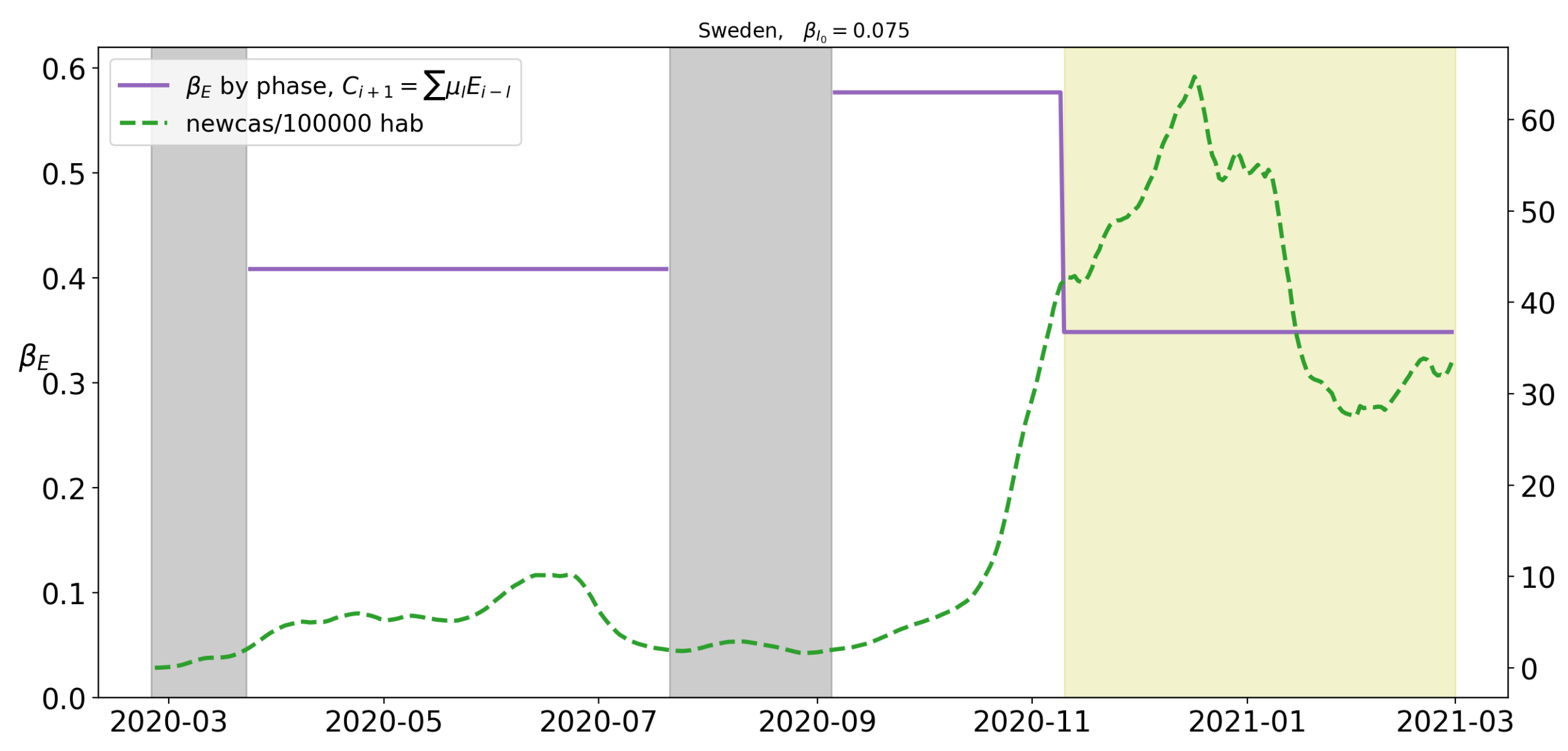
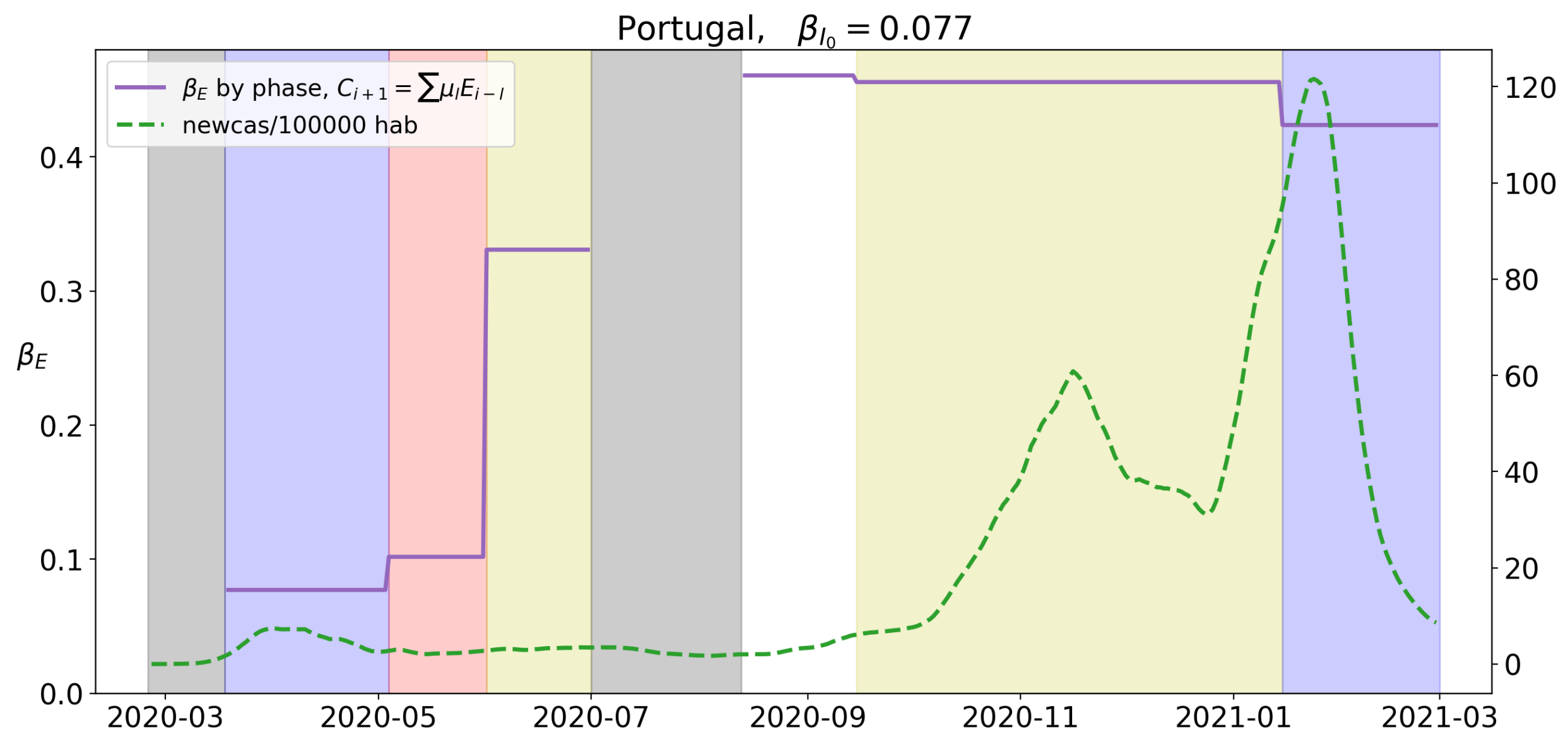
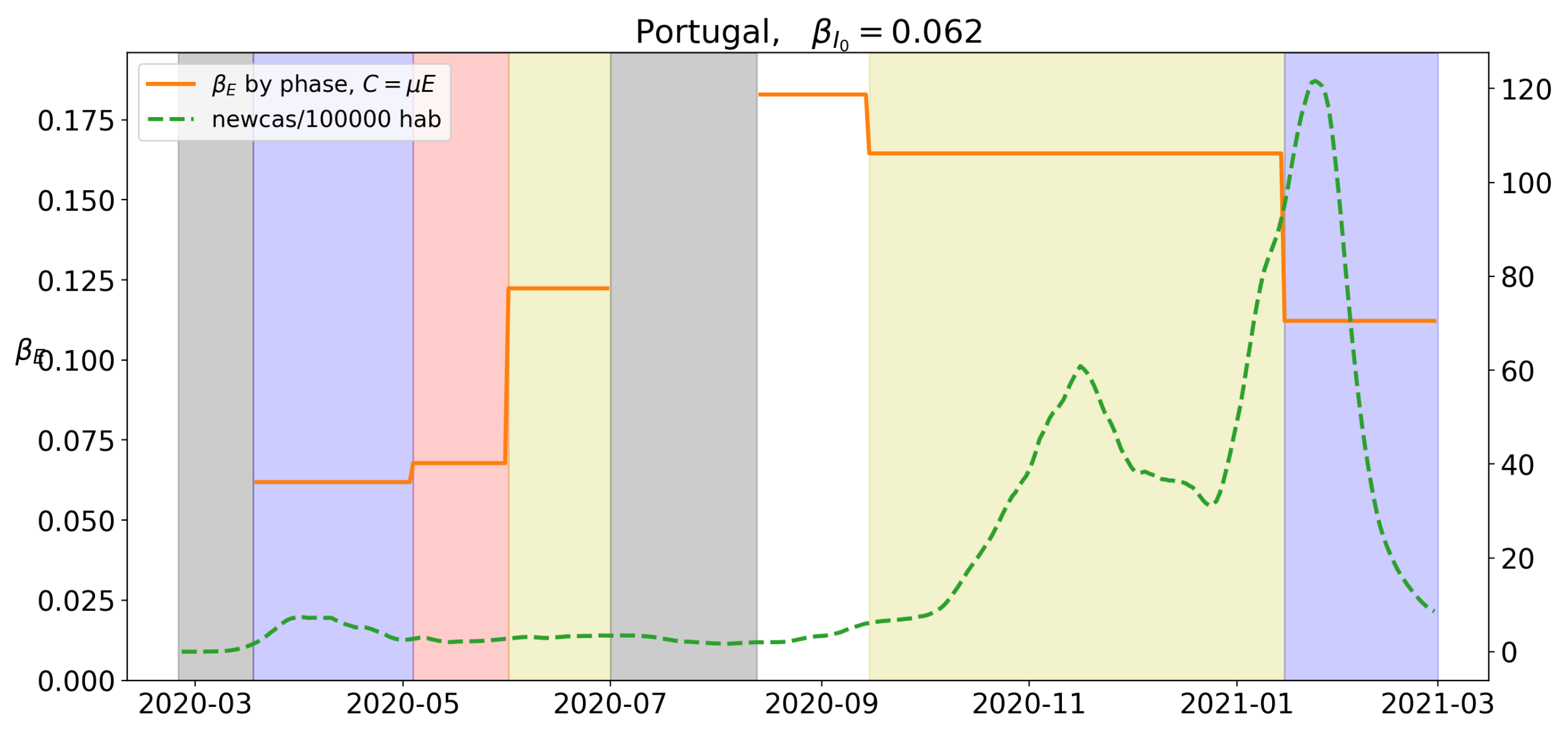
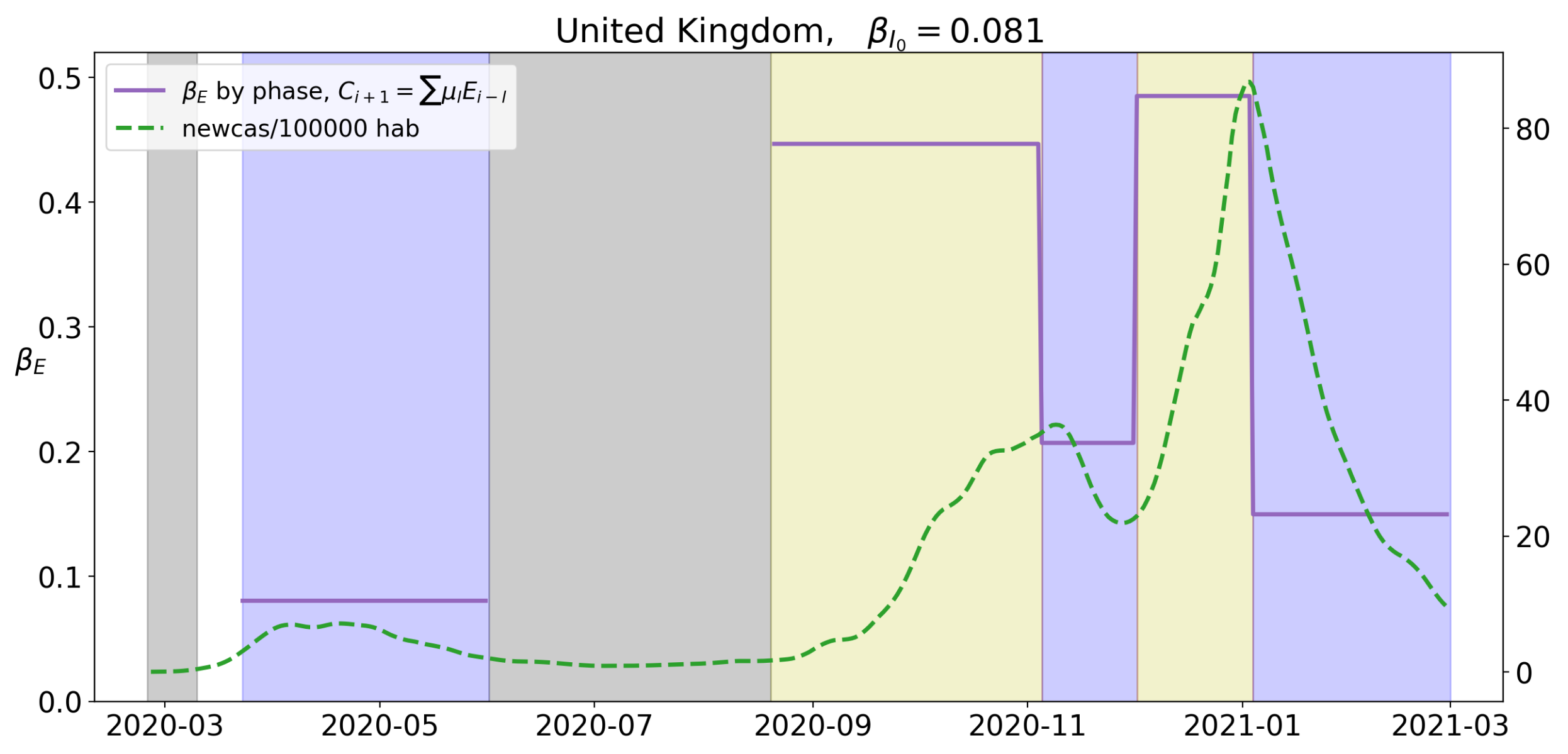
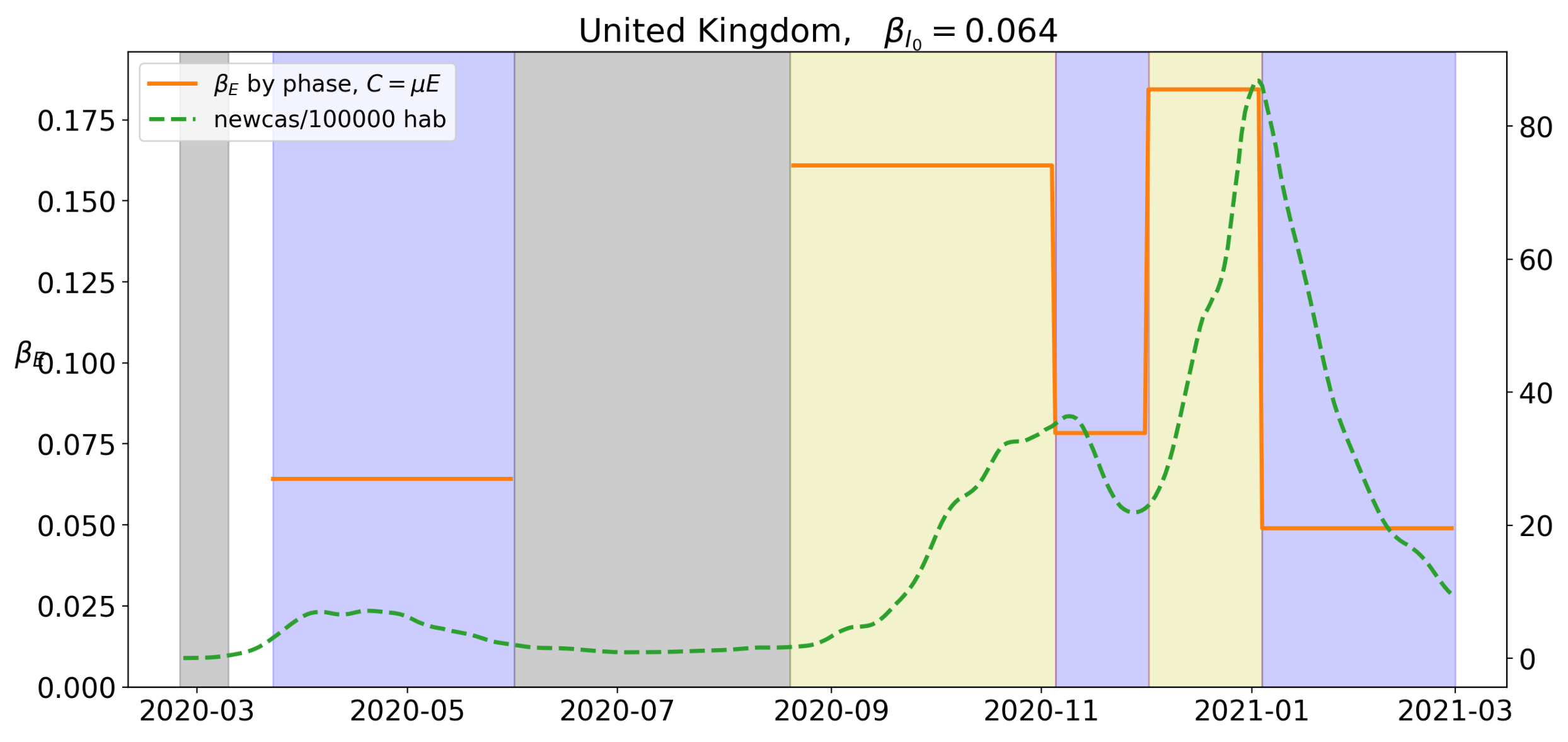
Figure 2.
Value of for the different levels of lockdown. Different k-values for reducing the are tried. Blue background will correspond to Stage 1, red to Stage 2, yellow to Stage 3 and white to Stage 4. A green dotted line corresponds to the value of new cases per 100,000 hab.
Figure 2.
Value of for the different levels of lockdown. Different k-values for reducing the are tried. Blue background will correspond to Stage 1, red to Stage 2, yellow to Stage 3 and white to Stage 4. A green dotted line corresponds to the value of new cases per 100,000 hab.
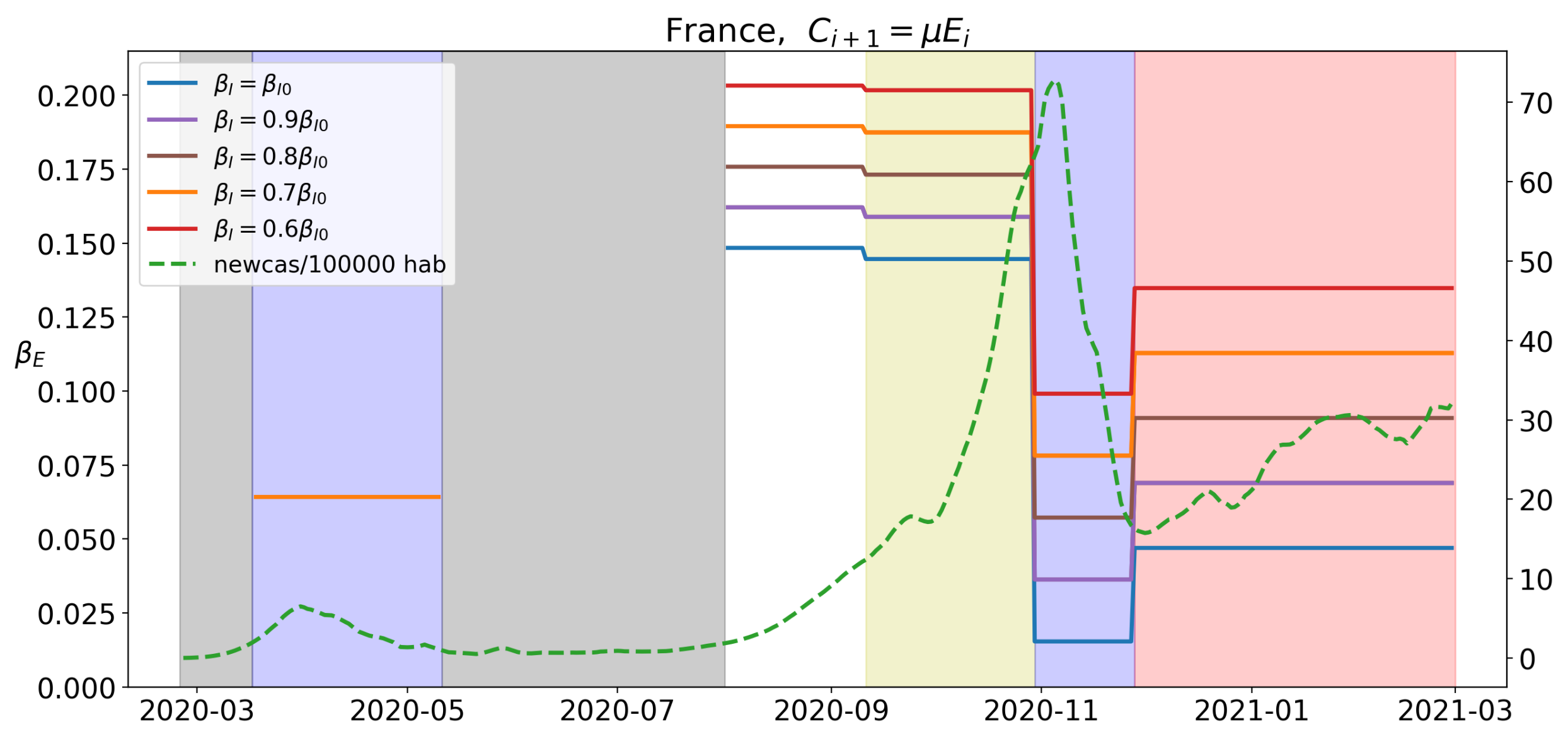
Figure 3.
Value of for the different levels of lockdown. Blue background will correspond to Stage 1, red to Stage 2, yellow to Stage 3 and white to Stage 4. A green dotted line corresponds to the value of new cases per 100,000 hab.
Figure 3.
Value of for the different levels of lockdown. Blue background will correspond to Stage 1, red to Stage 2, yellow to Stage 3 and white to Stage 4. A green dotted line corresponds to the value of new cases per 100,000 hab.
Figure 4.
Value of for the different levels of lockdown. Blue background will correspond to Stage 1, red to Stage 2, yellow to Stage 3 and white to Stage 4. A green dotted line corresponds to the value of new cases per 100,000 hab.
Figure 4.
Value of for the different levels of lockdown. Blue background will correspond to Stage 1, red to Stage 2, yellow to Stage 3 and white to Stage 4. A green dotted line corresponds to the value of new cases per 100,000 hab.
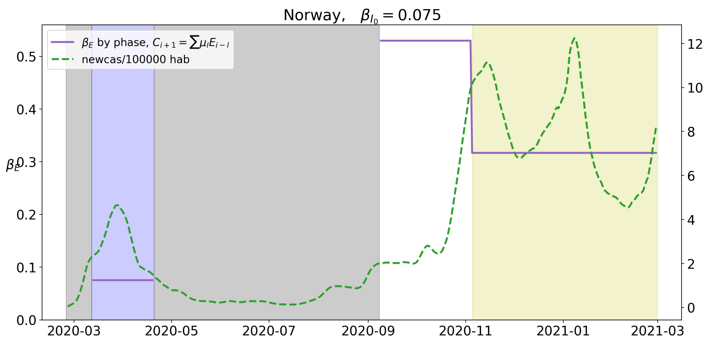
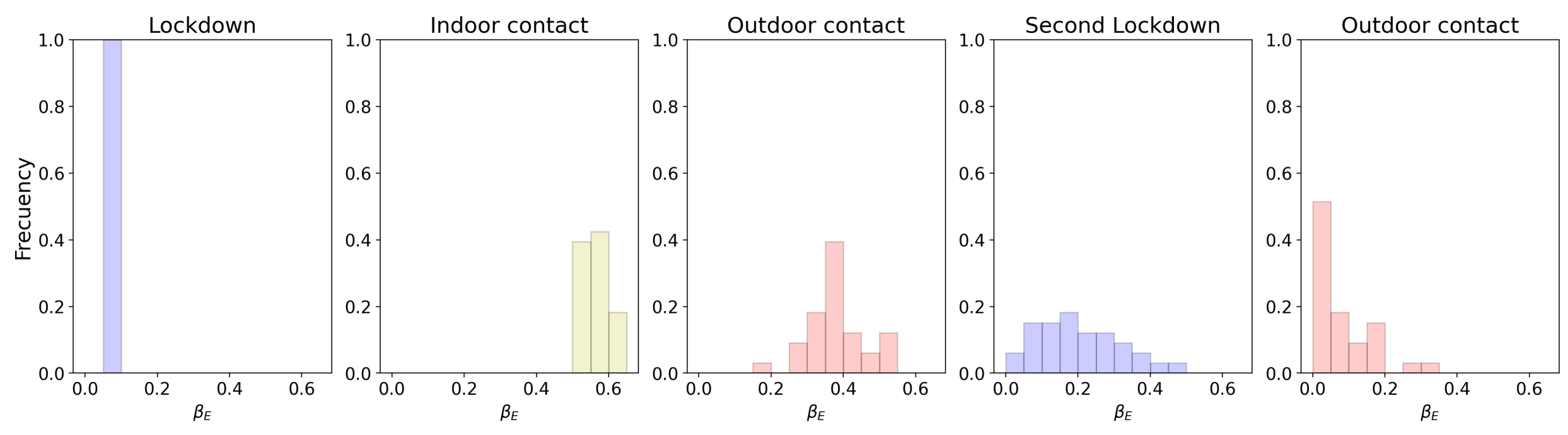
Figure 5.
Value of for the different levels of lockdown. Blue background will correspond to Stage 1, red to Stage 2, yellow to Stage 3 and white to Stage 4. A green dotted line corresponds to the value of new cases per 100,000 hab.
Figure 5.
Value of for the different levels of lockdown. Blue background will correspond to Stage 1, red to Stage 2, yellow to Stage 3 and white to Stage 4. A green dotted line corresponds to the value of new cases per 100,000 hab.
Figure 6.
Value of for the different levels of lockdown. Yellow background corresponds to a mild social distancing measure classified as Stage 3 and white background to “normality”, with no substantial self-isolation measures adopted. A green dotted line corresponds to the value of new cases per 100,000 hab.
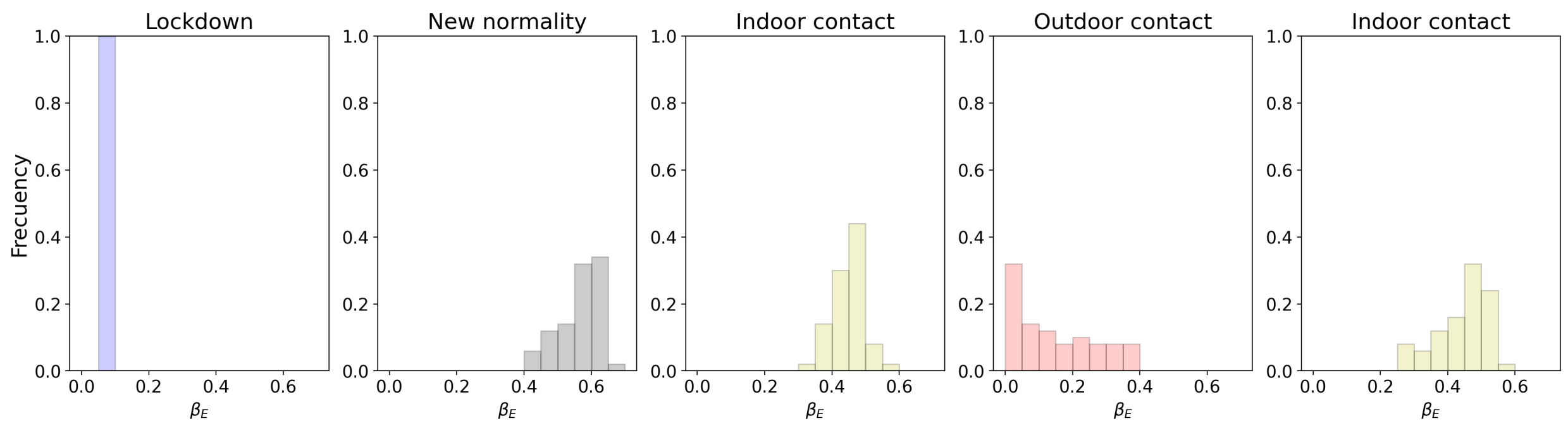
Figure 7.
Value of for the different levels of lockdown. Yellow backgrounds correspond to a mild social distancing measure classified as Stage 3 and white background to “normality”, with no substantial self-isolation measures adopted. A green dotted line corresponds to the value of new cases per 100,000 hab.
Figure 8.
Value of for the different levels of lockdown. Blue background will correspond to Stage 1, red to Stage 2, yellow to Stage 3 and white to Stage 4. A green dotted line corresponds to the value of new cases per 100,000 hab.
Figure 8.
Value of for the different levels of lockdown. Blue background will correspond to Stage 1, red to Stage 2, yellow to Stage 3 and white to Stage 4. A green dotted line corresponds to the value of new cases per 100,000 hab.
Figure 9.
Value of for the different levels of lockdown. Blue background will correspond to Stage 1, red to Stage 2, yellow to Stage 3 and white to Stage 4. A green dotted line corresponds to the value of new cases per 100,000 hab.
Figure 9.
Value of for the different levels of lockdown. Blue background will correspond to Stage 1, red to Stage 2, yellow to Stage 3 and white to Stage 4. A green dotted line corresponds to the value of new cases per 100,000 hab.
Figure 10.
Value of for the different levels of lockdown. Blue will correspond to Stage 1, yellow to Stage 3 and white to Stage 4. A green dotted line corresponds to the value of new cases per 100,000 hab.
Figure 10.
Value of for the different levels of lockdown. Blue will correspond to Stage 1, yellow to Stage 3 and white to Stage 4. A green dotted line corresponds to the value of new cases per 100,000 hab.
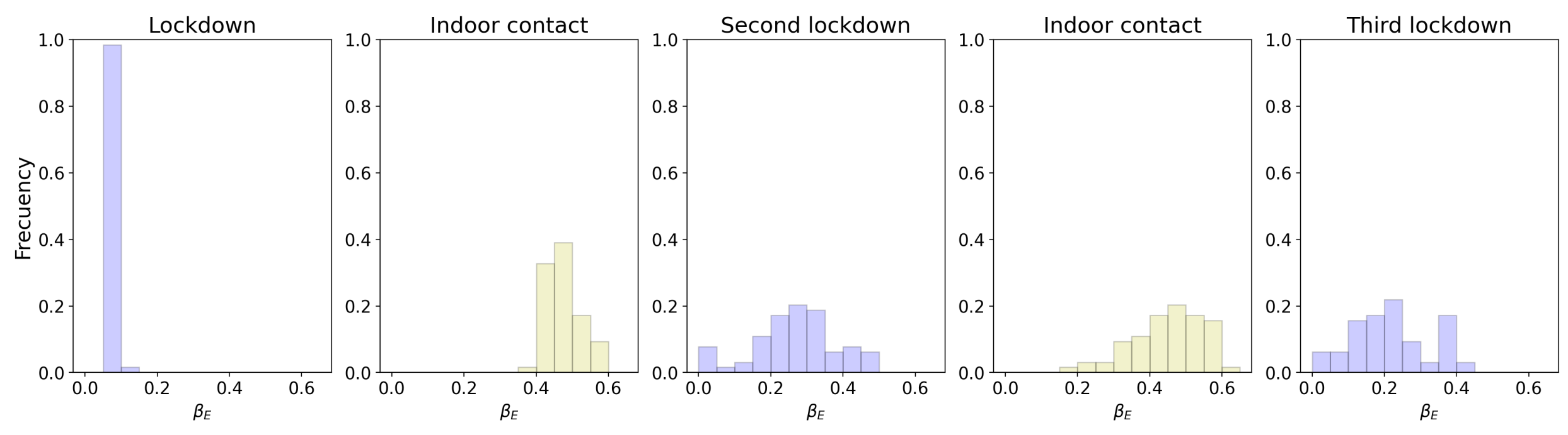
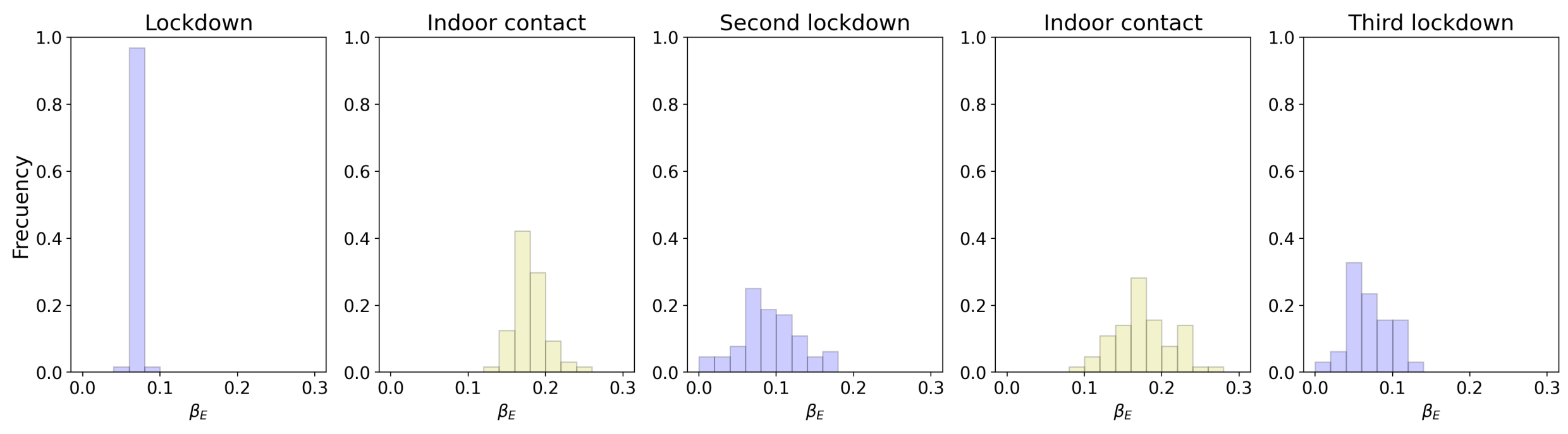
Figure 11.
Histogram of the 64 different counties of United Kingdom. The value of at the different levels of lockdown registered in 2020.
Figure 11.
Histogram of the 64 different counties of United Kingdom. The value of at the different levels of lockdown registered in 2020.
Figure 12.
Value of for the different levels of lockdown. Blue will correspond to Stage 1, yellow to Stage 3 and white to Stage 4. A green dotted line corresponds to the value of new cases per 100,000 hab.
Figure 12.
Value of for the different levels of lockdown. Blue will correspond to Stage 1, yellow to Stage 3 and white to Stage 4. A green dotted line corresponds to the value of new cases per 100,000 hab.
Figure 13.
Histogram of 64 different counties of United Kingdom. The value of at the different levels of lockdown registered in 2020.
Figure 13.
Histogram of 64 different counties of United Kingdom. The value of at the different levels of lockdown registered in 2020.
Figure 14.
Value of for the different levels of lockdown. Blue background will correspond to Stage 1, red to Stage 2, yellow to Stage 3 and white to Stage 4. A green dotted line corresponds to the value of new cases per 100,000 hab.
Figure 14.
Value of for the different levels of lockdown. Blue background will correspond to Stage 1, red to Stage 2, yellow to Stage 3 and white to Stage 4. A green dotted line corresponds to the value of new cases per 100,000 hab.
Figure 15.
Histogram of the 33 different regions of Germany. The value of at the different levels of lockdown registered in 2020.
Figure 15.
Histogram of the 33 different regions of Germany. The value of at the different levels of lockdown registered in 2020.
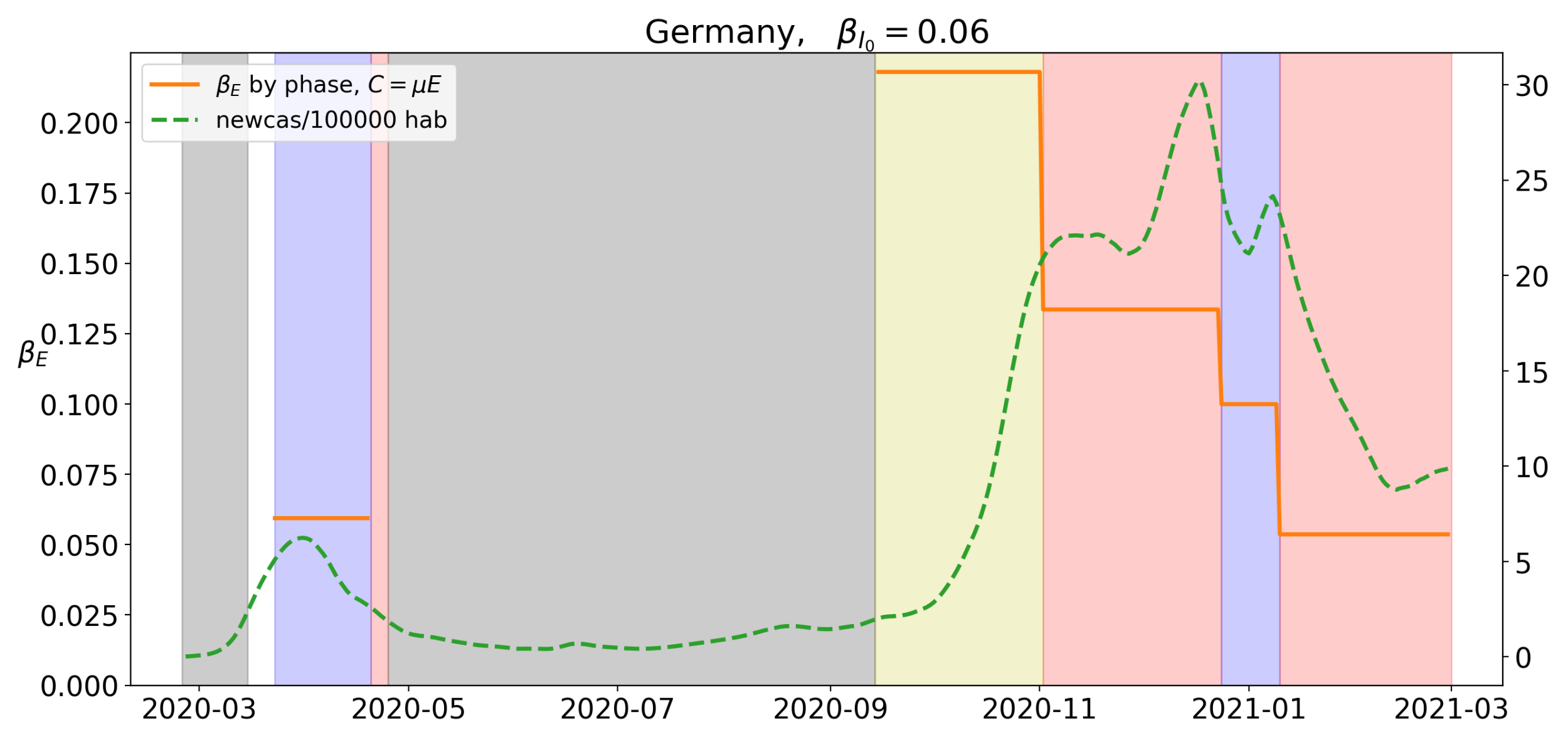
Figure 16.
Value of for the different levels of lockdown. Blue background will correspond to Stage 1, red to Stage 2, yellow to Stage 3 and white to Stage 4. A green dotted line corresponds to the value of new cases per 100,000 hab.
Figure 16.
Value of for the different levels of lockdown. Blue background will correspond to Stage 1, red to Stage 2, yellow to Stage 3 and white to Stage 4. A green dotted line corresponds to the value of new cases per 100,000 hab.
Figure 17.
Histogram of the 33 different regions of Germany. The value of at the different levels of lockdown registered in 2020.
Figure 17.
Histogram of the 33 different regions of Germany. The value of at the different levels of lockdown registered in 2020.
Figure 18.
Value of for the different levels of lockdown. Blue background will correspond to Stage 1, red to Stage 2, yellow to Stage 3 and white to Stage 4. A green dotted line corresponds to the value of new cases per 100,000 hab.
Figure 18.
Value of for the different levels of lockdown. Blue background will correspond to Stage 1, red to Stage 2, yellow to Stage 3 and white to Stage 4. A green dotted line corresponds to the value of new cases per 100,000 hab.
Figure 19.
Histogram of the 50 different provinces of Spain. The value of at the different levels of lockdown registered in 2020.
Figure 19.
Histogram of the 50 different provinces of Spain. The value of at the different levels of lockdown registered in 2020.
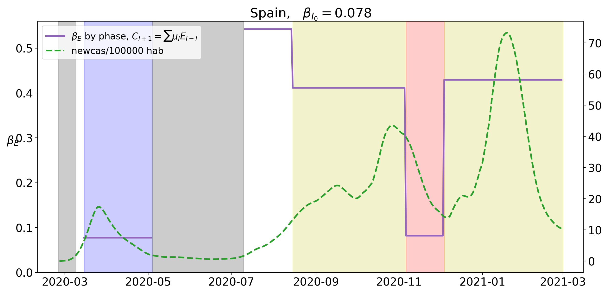
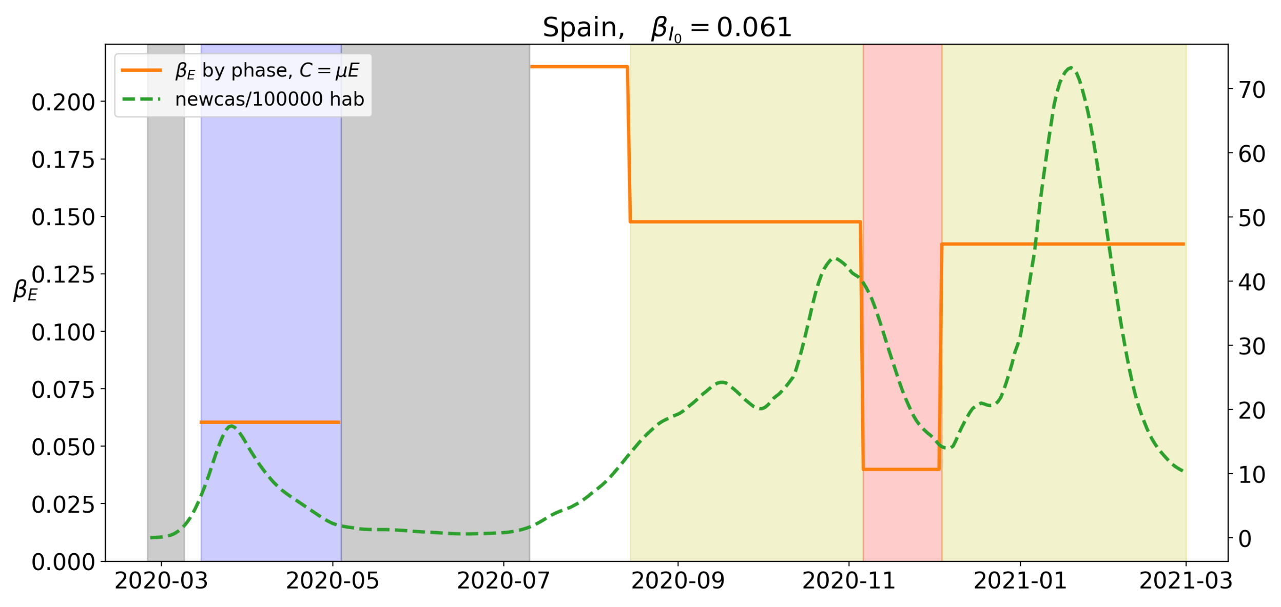
Figure 20.
Value of for the different levels of lockdown in Spain. Blue background will correspond to Stage 1, red to Stage 2, yellow to Stage 3 and white to Stage 4. A green dotted line corresponds to the value of new cases per 100,000 hab.
Figure 20.
Value of for the different levels of lockdown in Spain. Blue background will correspond to Stage 1, red to Stage 2, yellow to Stage 3 and white to Stage 4. A green dotted line corresponds to the value of new cases per 100,000 hab.
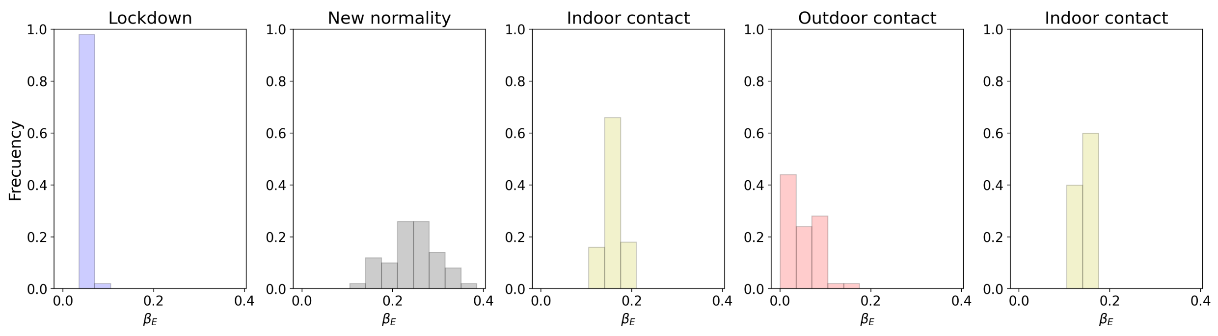
Figure 21.
Histogram of the 50 different provinces of Spain. The value of at the different levels of lockdown registered in 2020.
Figure 21.
Histogram of the 50 different provinces of Spain. The value of at the different levels of lockdown registered in 2020.
Figure 22.
Value of for the different levels of lockdown. Blue background will correspond to Stage 1, red to Stage 2, yellow to Stage 3 and white to Stage 4. A green dotted line corresponds to the value of new cases per 100,000 hab.
Figure 22.
Value of for the different levels of lockdown. Blue background will correspond to Stage 1, red to Stage 2, yellow to Stage 3 and white to Stage 4. A green dotted line corresponds to the value of new cases per 100,000 hab.
Figure 23.
Histogram of the 107 different regions of Italy. The value of at the different levels of lockdown registered in 2020.
Figure 23.
Histogram of the 107 different regions of Italy. The value of at the different levels of lockdown registered in 2020.
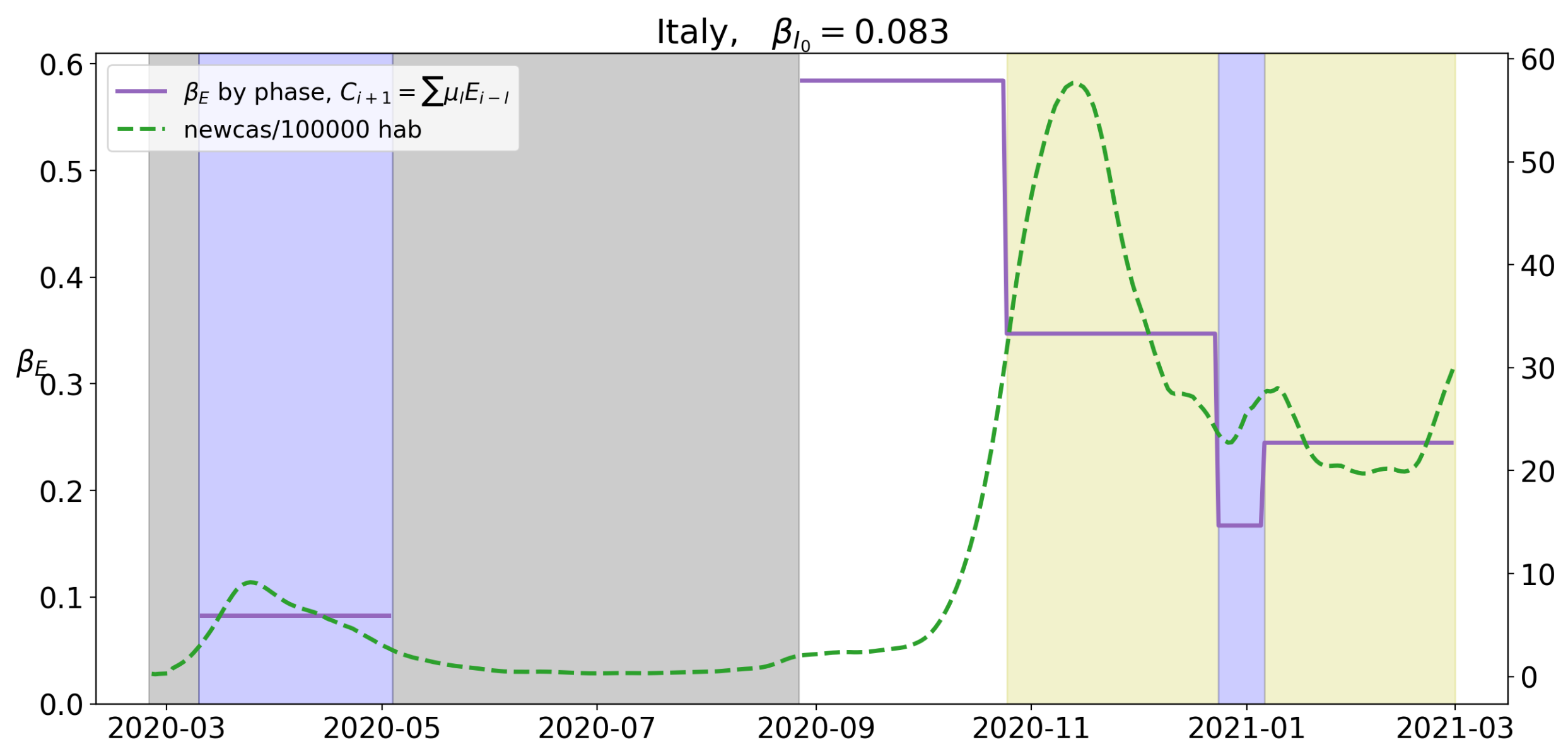
Figure 24.
Value of for the different levels of lockdown. Blue background will correspond to Stage 1, red to Stage 2, yellow to Stage 3 and white to Stage 4. A green dotted line corresponds to the value of new cases per 100,000 hab.
Figure 24.
Value of for the different levels of lockdown. Blue background will correspond to Stage 1, red to Stage 2, yellow to Stage 3 and white to Stage 4. A green dotted line corresponds to the value of new cases per 100,000 hab.
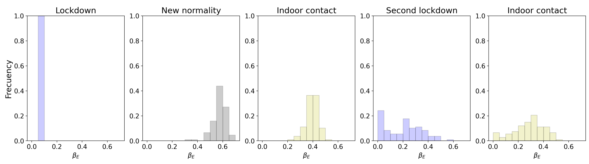
Figure 25.
Histogram of the 107 different regions of Italy. The value of at the different levels of lockdown registered in 2020.
Figure 25.
Histogram of the 107 different regions of Italy. The value of at the different levels of lockdown registered in 2020.
Table 1.
Data for France: Total cases, Cases per 100,000 inhabitants in the last 14 days, rate of Cases in the last 14 days and the previous 14 days interval, Death related to COVID-19.
Table 1.
Data for France: Total cases, Cases per 100,000 inhabitants in the last 14 days, rate of Cases in the last 14 days and the previous 14 days interval, Death related to COVID-19.
| Date | Total Cases | I | | Death |
|---|
| 17 March 2020 | 7730 | 11.2 | 37.6 | 225 |
| 11 May 2020 | 139,519 | 16.7 | 0.5 | 26,643 |
| 1 August 2020 | 189,547 | 20.7 | 1.9 | 30,251 |
| 11 September 2020 | 363,350 | 143.5 | 1.9 | 30,893 |
| 30 October 2020 | 1,331,984 | 741.4 | 2.2 | 36,565 |
| 28 November 2020 | 2,208,699 | 378.9 | 0.5 | 52,127 |
| 12 February 2021 | 3,427,386 | 408.4 | 1.0 | 81,448 |
Table 2.
Data for Norway: Total cases, Cases per 100,000 inhabitants in the last 14 days, rate of Cases in the last 14 days and the previous 14 days interval, Death related to COVID-19.
Table 2.
Data for Norway: Total cases, Cases per 100,000 inhabitants in the last 14 days, rate of Cases in the last 14 days and the previous 14 days interval, Death related to COVID-19.
| Date | Total Cases | I | | Death |
|---|
| 12 March 2020 | 860 | 15.9 | 15.9 | 0 |
| 20 April 2020 | 7106 | 25.1 | 0.4 | 154 |
| 8 September 2020 | 11,448 | 20.9 | 1.8 | 264 |
| 5 November 2020 | 22,467 | 104.2 | 3.2 | 284 |
| 12 February 2021 | 65,457 | 65.6 | 0.9 | 592 |
Table 3.
Data for Sweden: Total cases, Cases per 100,000 inhabitants in the last 14 days, rate of Cases in the last 14 days and the previous 14 days interval, Death related to COVID-19.
Table 3.
Data for Sweden: Total cases, Cases per 100,000 inhabitants in the last 14 days, rate of Cases in the last 14 days and the previous 14 days interval, Death related to COVID-19.
| Date | Total Cases | I | | Death |
|---|
| 23 March 2020 | 2169 | 17.8 | 5.7 | 33 |
| 21 July 2020 | 74,766 | 35.1 | 0.4 | 5670 |
| 5 September 2020 | 85,500 | 24.4 | 0.7 | 5848 |
| 10 November 2020 | 166,956 | 470.7 | 1.6 | 6092 |
| 12 February 2021 | 609,306 | 400.1 | 1.0 | 12,449 |
Table 4.
Data for Portugal: Total cases, Cases per 100,000 inhabitants in the last 14 days, rate of Cases in the last 14 days and the previous 14 days interval, Death related to COVID-19.
Table 4.
Data for Portugal: Total cases, Cases per 100,000 inhabitants in the last 14 days, rate of Cases in the last 14 days and the previous 14 days interval, Death related to COVID-19.
| Date | Total Cases | I | | Death |
|---|
| 23 March 2020 | 642 | 6.2 | 106 | 1 |
| 4 May 2020 | 25,524 | 45.3 | 0.6 | 1063 |
| 1 July 2020 | 42,523 | 47.1 | 1.2 | 1579 |
| 15 September 2020 | 65,021 | 65.8 | 1.9 | 1875 |
| 15 January 2021 | 528,469 | 1047.4 | 2.2 | 8543 |
| 12 February 2021 | 781,223 | 802.6 | 0.5 | 15,034 |
Table 5.
Data for the UK: Total cases, Cases per 100,000 inhabitants in the last 14 days, rate of change of I in 14 days, Death related to COVID-19.
Table 5.
Data for the UK: Total cases, Cases per 100,000 inhabitants in the last 14 days, rate of change of I in 14 days, Death related to COVID-19.
| Date | Total Cases | I | | Death |
|---|
| 23 March 2020 | 12,639 | 18 | 19.9 | 938 |
| 1 June2020 | 257,702 | 37.9 | 0.7 | 38,294 |
| 20 August 2020 | 325,468 | 22.37 | 1.4 | 41,494 |
| 5 November 2020 | 1,183,510 | 464.9 | 1.3 | 49,271 |
| 2 December 2020 | 1,696,375 | 317.5 | 0.7 | 61,050 |
| 4 January 2021 | 2,880,767 | 1042.7 | 1.8 | 79,323 |
| 12 February 2021 | 4,040,037 | 328.2 | 0.6 | 118,097 |
Table 6.
Histogram for the mean values of at the different stages of lockdown in the UK.
Table 6.
Histogram for the mean values of at the different stages of lockdown in the UK.
| Phase | Mean | Variance | CI 95% | p |
|---|
| Lockdown | 0.08 | | (80.7, 82.5) |
| Indoor contact | 0.46 | 12 | (452.6, 469.5) | 0 |
| Second lockdown | 0.22 | 134 | (192.0, 248.6) | 0 |
| Indoor contact | 0.47 | 80 | (452.0, 495.7) | 0 |
| Third lockdown | 0.17 | 69 | (144.8, 185.4) | 0 |
Table 7.
Histogram for the mean values of at the different stages of lockdown in the UK.
Table 7.
Histogram for the mean values of at the different stages of lockdown in the UK.
| Phase | Mean | Variance | CI 95% | p |
|---|
| Lockdown | | | (64, 66) |
| Indoor contact | | | (164, 173) | 0 |
| Second lockdown | | | (74, 93) | 0 |
| Indoor contact | | | (178, 194) | 0 |
| Third lockdown | | | (48, 59) | 0 |
Table 8.
Data for Germany: Total cases, Cases per 100,000 inhabitants in the last 14 days, rate of Cases in the last 14 days and the previous 14 days interval, Death related to COVID-19.
Table 8.
Data for Germany: Total cases, Cases per 100,000 inhabitants in the last 14 days, rate of Cases in the last 14 days and the previous 14 days interval, Death related to COVID-19.
| Date | Total Cases | I | | Death |
|---|
| 23 March 2020 | 35,985 | 40.8 | 16.3 | 708 |
| 20 April 2020 | 146,504 | 50.5 | 0.6 | 7537 |
| 14 September 2020 | 264,405 | 23.1 | 1.2 | 9593 |
| 2 November 2020 | 579,340 | 234.8 | 2.7 | 13,417 |
| 24 December 2020 | 1,614,002 | 397.52 | 1.3 | 43,701 |
| 10 January 2021 | 1,933,486 | 315.9 | 0.9 | 55,945 |
| 12 February 2021 | 2,326,814 | 147.8 | 0.7 | 69,327 |
Table 9.
Histogram for the mean values of at the different stages of lockdown in Germany.
Table 9.
Histogram for the mean values of at the different stages of lockdown in Germany.
| Phase | Mean | Variance | CI 95% | p |
|---|
| Lockdown | | | (78, 79) | |
| Indoor contact | | | (557, 579) | 0 |
| Outdoor contact | | | (355, 407) | 0 |
| Second Lockdown | | | (176, 252) | < |
| Outdoor contact | | | (53, 111) | < |
Table 10.
Histogram for the mean values of at the different stages of lockdown in Germany.
Table 10.
Histogram for the mean values of at the different stages of lockdown in Germany.
| Phase | Mean | Variance | CI 95% | p |
|---|
| Lockdown | | | (5.9, 6.0) | |
| Indoor contact | | | (21.7, 22.6) | 0 |
| Outdoor contact | | | (12.8, 14.5) | 0 |
| Second Lockdown | | | (8.8, 11.0) | < |
| Outdoor contact | | | (4.3, 6.1) | < |
Table 11.
Data for Spain: Total cases, Cases per 100,000 inhabitants in the last 14 days, rate of Cases in the last 14 days and the previous 14 days interval, Death related to COVID-19.
Table 11.
Data for Spain: Total cases, Cases per 100,000 inhabitants in the last 14 days, rate of Cases in the last 14 days and the previous 14 days interval, Death related to COVID-19.
| Date | Total Cases | I | | Death |
|---|
| 15 March 2020 | 12,874 | 26.9 | 108.9 | 508 |
| 4 May 2020 | 228,788 | 44.9 | 0.5 | 26,878 |
| 10 July 2020 | 266,181 | 16.6 | 1.8 | 29,796 |
| 15 August 2020 | 383,287 | 145.6 | 1.9 | 30,245 |
| 6 November 2020 | 1,453,433 | 619.4 | 1.4 | 41,167 |
| 4 December 2020 | 1,781,385 | 246.2 | 0.6 | 48,580 |
| 12 February 2021 | 3,106,326 | 471.2 | 0.5 | 66,858 |
Table 12.
Histogram for the mean values of at the different stages of lockdown in Spain.
Table 12.
Histogram for the mean values of at the different stages of lockdown in Spain.
| Phase | Mean | Variance | CI 95% | p |
|---|
| Lockdown | | | (7.6, 7.9) | |
| New normality | | | (55.5, 58.9) | 0 |
| Indoor contact | | | (41.8, 44.8) | 0 |
| Outdoor contact | | | (11.7, 19.6) | 0 |
| Indoor contact | | | (41.7, 49.0) | 0 |
Table 13.
Histogram for the mean values of at the different stages of lockdown in Spain.
Table 13.
Histogram for the mean values of at the different stages of lockdown in Spain.
| Phase | Mean | Variance | CI 95% | p |
|---|
| Lockdown | | | (6.0, 6.1) | |
| New normality | | | (23.0, 25.9) | 0 |
| Indoor contact | | | (14.9, 16.0) | 0 |
| Outdoor contact | | | (4.0, 6.2) | 0 |
| Indoor contact | | | (15.6, 19.0) | 0 |
Table 14.
Data for Italy: Total cases, Cases per 100,000 inhabitants in the last 14 days, rate of Cases in the last 14 days and the previous 14 days interval, Death related to COVID-19.
Table 14.
Data for Italy: Total cases, Cases per 100,000 inhabitants in the last 14 days, rate of Cases in the last 14 days and the previous 14 days interval, Death related to COVID-19.
| Date | Total Cases | I | | Death |
|---|
| 10 March 2020 | 10,149 | 16.3 | 31.1 | 631 |
| 4 May 2020 | 211,938 | 50.9 | 0.7 | 29,079 |
| 27 August 2020 | 263,949 | 19.4 | 2.5 | 35,463 |
| 25 October 2020 | 525,782 | 283.2 | 3.9 | 37,338 |
| 24 December 2020 | 2,009,317 | 368.3 | 0.9 | 70,900 |
| 6 January 2021 | 2,201,945 | 349.3 | 1.0 | 76,877 |
| 12 February 2021 | 2,697,296 | 278.9 | 1.1 | 93,045 |
Table 15.
Histogram for the mean values of at the different stages of lockdown in Italy.
Table 15.
Histogram for the mean values of at the different stages of lockdown in Italy.
| Phase | Mean | Variance | CI 95% | p |
|---|
| Lockdown | 0.079 | | (7.8, 8.0) | |
| New normality | 0.568 | | (55.9, 57.6) | 0 |
| Indoor contact | 0.399 | | (39.0, 40.9) | 0 |
| Second lockdown | 0.206 | | (17.7, 23.4) | 0 |
| Indoor contact | 0.268 | | (24.5, 29.2) | < |
Table 16.
Histogram for the mean values of at the different stages of lockdown in Italy.
Table 16.
Histogram for the mean values of at the different stages of lockdown in Italy.
| Phase | Mean | Variance | CI 95% | p |
|---|
| Lockdown | | | (6.1, 6.2) | |
| New normality | | | (25.6, 26.9) | 0 |
| Indoor contact | | | (12.7, 13.2) | 0 |
| Second lockdown | | | (10.4, 12.4) | |
| Indoor contact | | | (9.5, 11.0) | |


 ,
, 


