Directed Energy Deposition-Arc (DED-Arc) and Numerical Welding Simulation as a Hybrid Data Source for Future Machine Learning Applications

Abstract

This research presents a hybrid approach to generate sample data for future machine learning applications for the prediction of mechanical properties in directed energy deposition-arc (DED-Arc) using the GMAW process. DED-Arc is an additive manufacturing process which offers a cost-effective way to generate 3D metal parts, due to its high deposition rate of up to 8 kg/h. The mechanical properties additively manufactured wall structures made of the filler material G4Si1 (ER70 S-6) are shown in dependency of the t_8/5 cooling time. The numerical simulation is used to link the process parameters and geometrical features to a specific t_8/5 cooling time. With an input of average welding power, welding speed and geometrical features such as wall thickness, layer height and heat source size a specific temperature field can be calculated for each iteration in the simulated welding process. This novel approach allows to generate large, artificial data sets as training data for machine learning methods by combining experimental results to generate a regression equation based on the experimentally measured t_8/5 cooling time. Therefore, using the regression equations in combination with numerically calculated t_8/5 cooling times an accurate prediction of the mechanical properties was possible in this research with an error of only 2.6%. Thus, a small set of experimentally generated data set allows to achieve regression equations which enable a precise prediction of mechanical properties. Moreover, the validated numerical welding simulation model was suitable to achieve an accurate calculation of the t_8/5 cooling time, with an error of only 0.3%.

1. Introduction

Additive manufacturing processes for metallic parts is a continuously growing market, with a growth of 41.9% in 2018 [1]. The manufacturing of metals includes different technologies, such as powder bed fusion (PBF) or direct energy deposition (DED). The difference between these processes is between the form of the deployed material (powder or wire) and the employed power source (electron beam, laser or electric arc) [2]. These differentiations not only result in varying near net shape, surface roughness or waviness of the additively manufactured part, but also in varying build-up rates and productivity of the used additive manufacturing process.

Directed energy deposition-arc (DED-Arc) can utilize gas metal arc welding (GMAW), the tungsten inert gas welding (TIG), as well as plasma processes during additive manufacturing. In these processes, a layer-by-layer structure is realized by feeding and melting a wire-shaped filler material. This process enables the generation of undercuts, cavities for lightweight construction applications or any cooling channels running in the component which cannot be produced or can only be produced to a limited extent using conventional methods (e.g., [3,4]). The GMAW process is particularly characterized by its cost-effective and robust process technology for additive manufacturing. DED-Arc using the arc GMAW process can achieve deposition rates of up to 8 kg/h, depending on the material and component geometry [5,6,7,8].

Due to the local inert gas cover, there are no restrictions of workspace size. In addition, the coaxial supply of filler material makes it possible to work independently of direction. Therefore, the only limitation of the buildable volume is the handling system. Thus, large scale components can be produced using the DED-Arc process [6,9]. Though, due to comparatively large melt pool sizes, the dimensional accuracy and surface quality are limited. Therefore, subtractive post-processing of the manufactured parts, at least for functional surfaces, is necessary to meet the required tolerances [5,10,11]. Figure 1 shows an example of a DED-Arc process chain.

The additive manufacturing of metal parts has been used in recent years to produce aerospace parts or for high-performance applications in the energy sector. Thus, nickel-base alloys [12,13] and titanium alloys [14,15] gained increasing interest in the last years. Therefore, the development of cost efficient production systems [16] which are capable of high deposition rates increases the chance for enterprises to enter fields such as architecture or construction engineering. Moreover, this allows freedom of design for complex 3D-structures such as architecture or construction engineering [17,18,19,20]. Recent investigations on a variety of materials such as low-alloyed steel [21,22,23,24], high-alloyed steel [25,26], hot work tool steel [27] or aluminum [28,29], in addition to the mentioned titanium and nickel base alloys, demonstrate the potential of this technology.

The high and recurring energy input during the DED-Arc process causes a complex thermal profile, residual stress and deformations. Finite element methods can provide the opportunity to study mitigation strategies for thermo-mechanical problems introduced by the DED-Arc, such as recurring thermal cycles and distortion, or to provide insights on the effect of a heat source on thermal behavior. Therefore, these complex interaction can provide a better method to explain the correlation between thermal cycles and mechanical properties due to transient data for the whole simulated part [30,31,32,33,34,35,36,37,38].

Deep learning methods have achieved remarkable success in many fields, such as computer vision and speech processing. Machine learning algorithms are usually more efficient the more data they have access to, and therefore heavily rely on large data sets [39,40,41]. Unfortunately for many processes, including DED-Arc, there is only a small amount of data available to effectively use machine learning methods. In DED-Arc, the sample sizes are generally fairly low, due to the high amount of time needed for manufacturing, sample preparation and testing. The labeling of the data is particularly time consuming. Data augmentation can be an effective tool to enhance the training data size and quality. The main idea of data augmentation is to generate synthetic data for untested parameter sets to cover unexplored areas of the parameter matrix [41].

In Jaeckel et al., data augmentation for machine learning through numerical analysis was shown to be a viable tool to extend a small data set to a comprehensive database for semi-tubular self-pierce riveting as a mechanical joining process [42]. Zhang et al. used data augmentation, such as adding noise and image rotation, to enhance the data set for training convolutional neural networks (CNN) for online defect detection in aluminum weld beads in robotic arc welding. Their research showed that they were able to achieve a classification accuracy of 99.38% [43]. Pu et al. tested different heat source models and their prediction accuracy of residual stress and deformation in butt-welded joints. It was found that the moving heat source model matched the measured welding deformation, whereas instantaneous heat source models had a poor accuracy for the deformation prediction [44]. Rikken et al. demonstrated how data fusion of simulation and experimental data can provide new insights about residual stress in welding applications. It was shown that accurate predictions of through-thickness residual stress state is possible, due to the combination of detailed material research, thermal analysis and sound mechanical simulation of a welding process [45].

In the introduction it was shown that there does not exist research combining achievable mechanical properties for DED-Arc processes and the use of numerical simulation to enhance methods of data augmentation to artificially generate a broader training data set. Therefore, the scope of this investigation is to build the basis for additional research on data augmentation for machine learning applications for DED-Arc processes to increase the number of artificial training data sets using transient thermal welding simulations. This will generate more data of t_8/5 cooling times to predict mechanical properties using regression equations, which are developed with a relatively small experimental data set. With this novel approach, data from simple wall structures to more complex three-dimensional ones can be calculated using a validated numerical simulation. This simulation predicts the properties of complex structures for which it might not be possible to extract samples for tensile or hardness test.

2. Materials and Methods

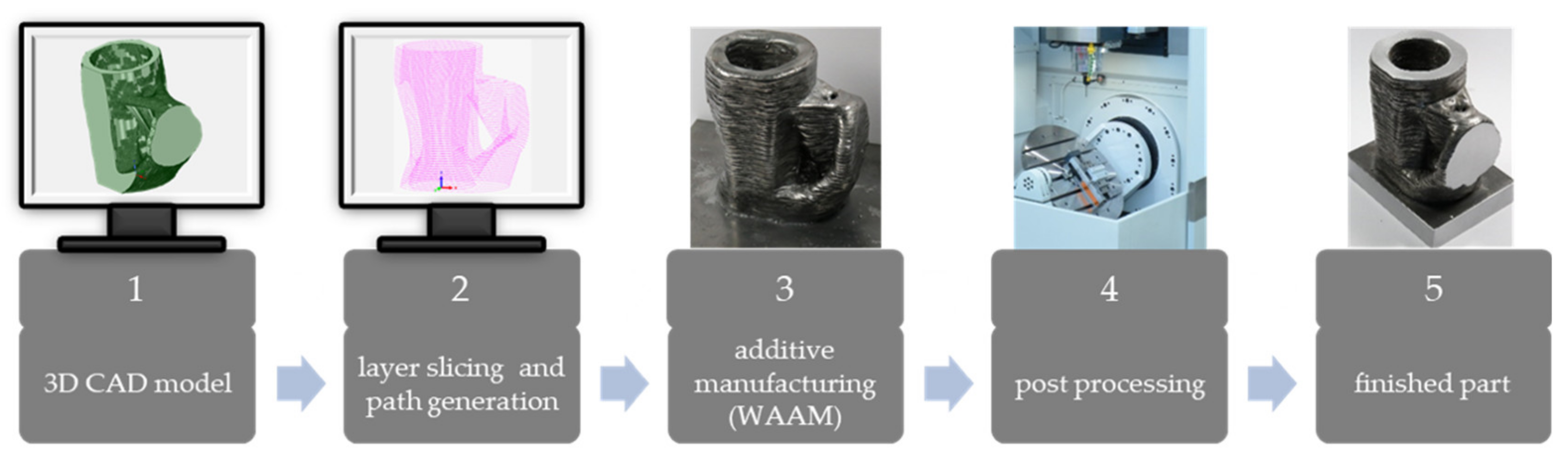
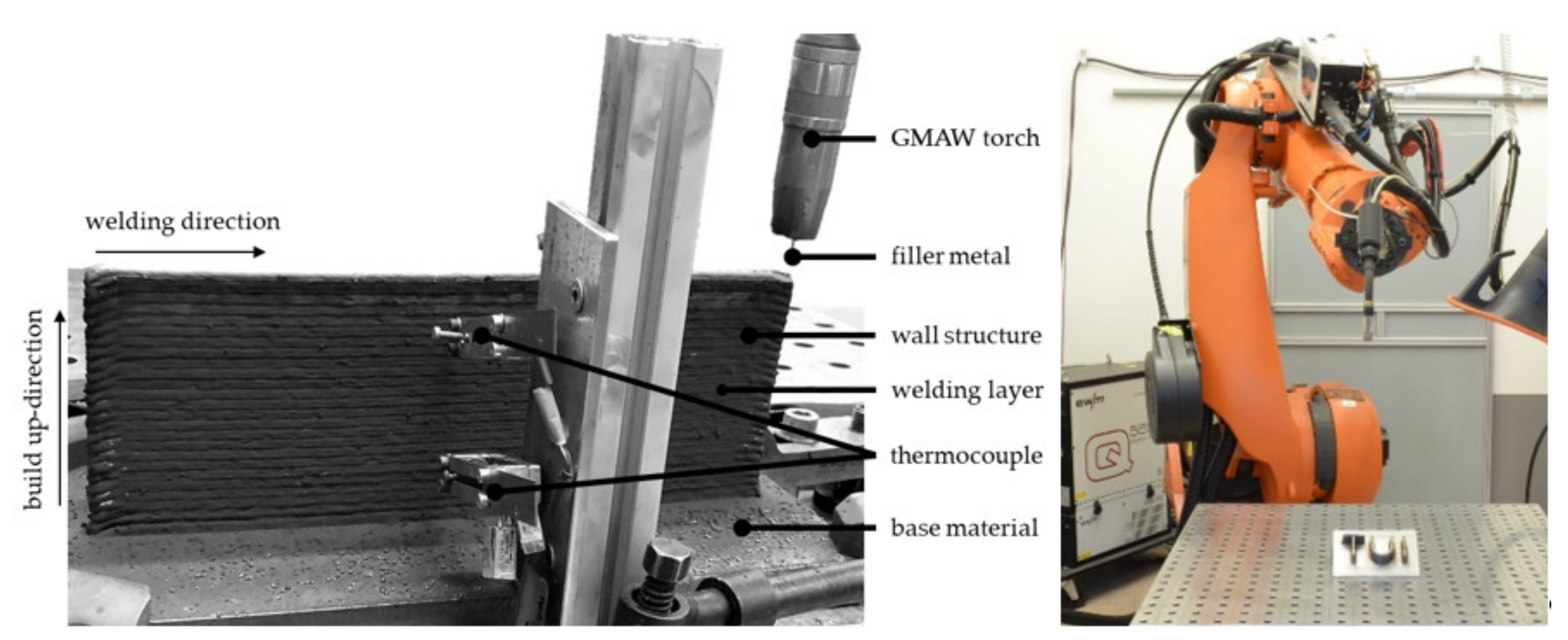
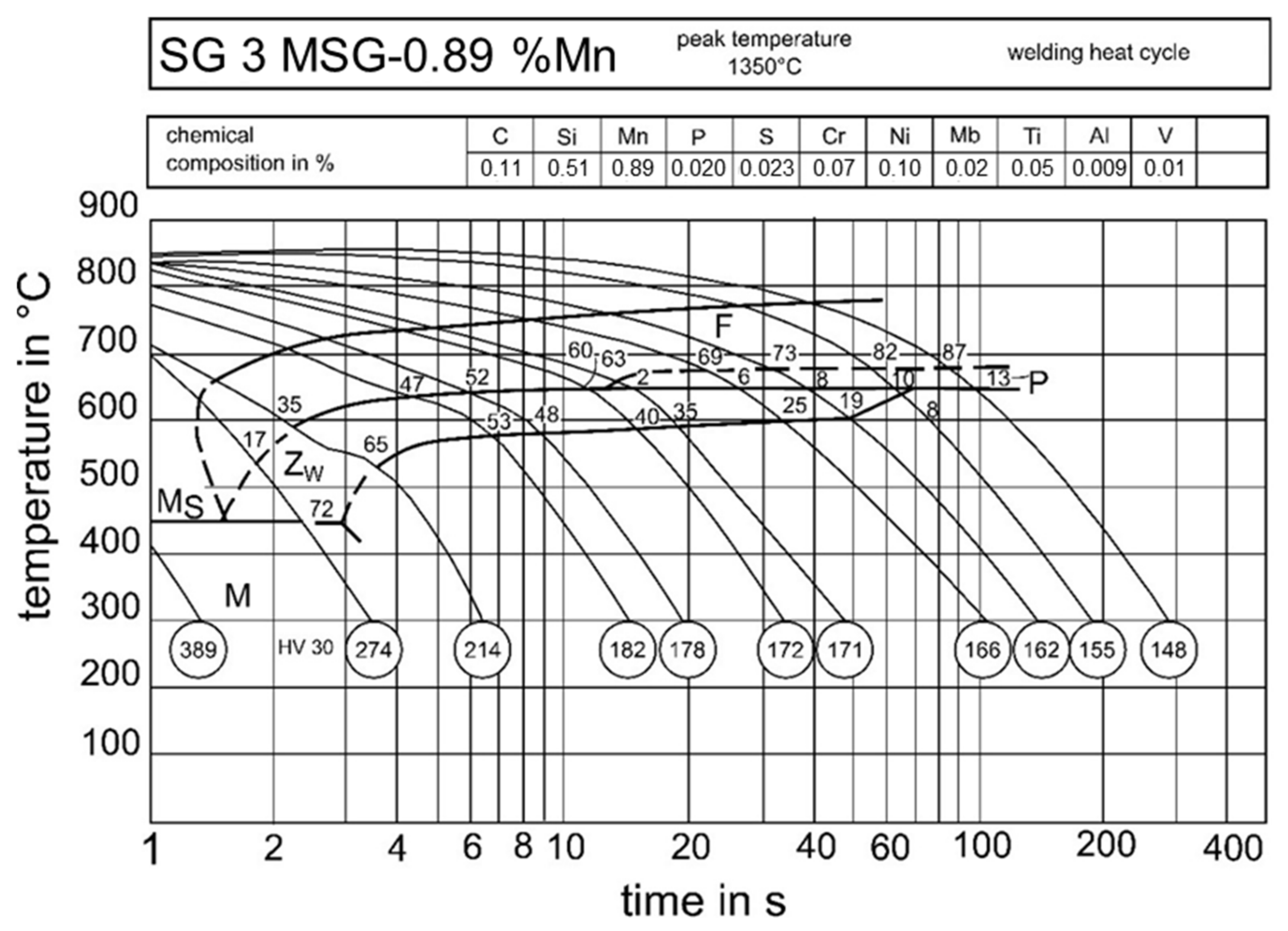
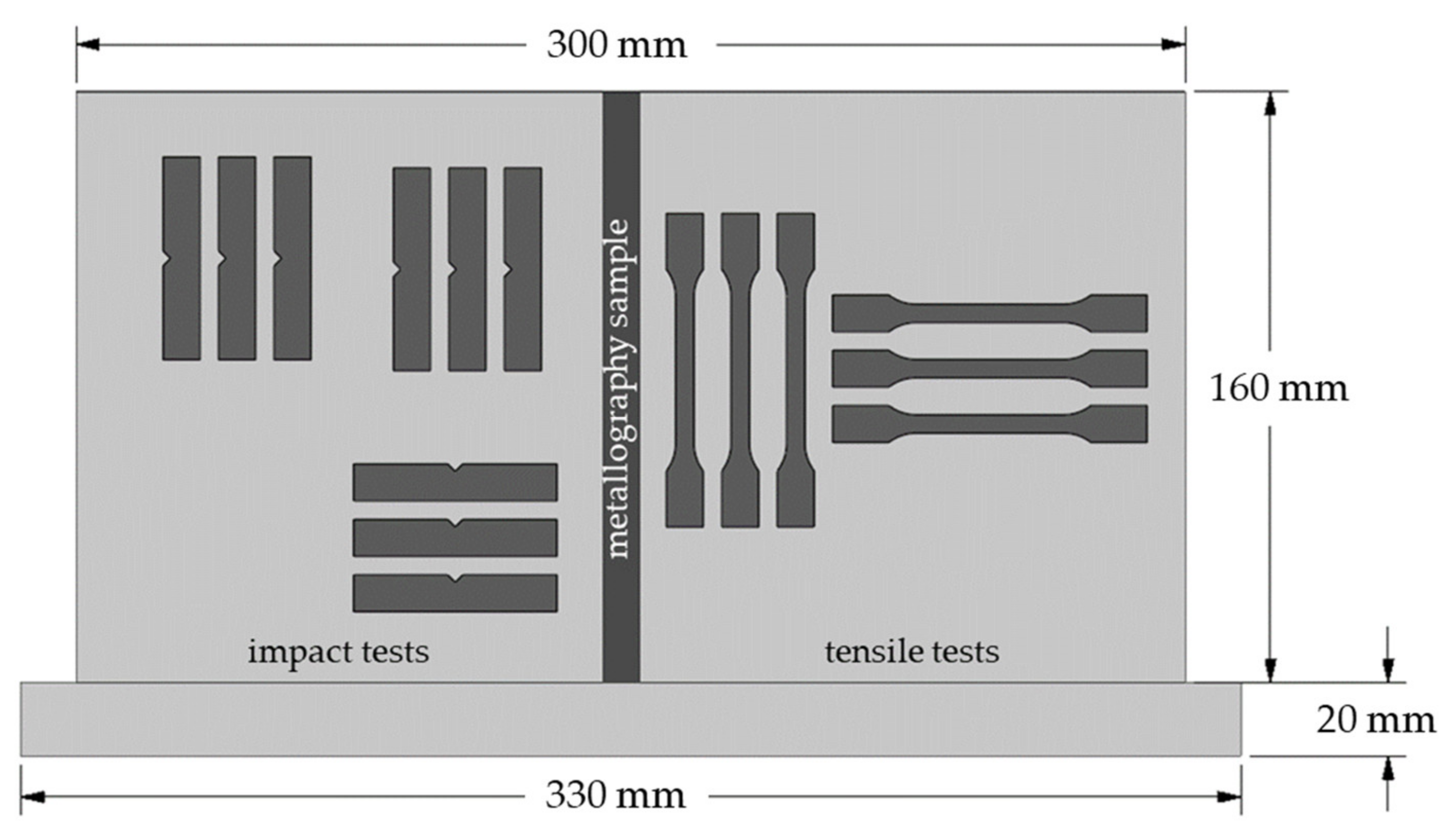
2.1. Materials and Additive Manufacturing

The additive generation of sample wall structures were carried out using an GMAW welding power source “EWM alpha Q 552 Expert 2.0 puls MM” with the energy-reduced short arc technology “coldArc”. A 6-axis industrial articulated arm robot “Kuka KR150-2” was used to ensure reproducible torch movement. The samples were generated using the low-alloyed solid wire electrode DIN EN ISO 14341-A-G4Si1 (ER70 S-6) to generate the wall structures and S355J2 + N with a thickness of 20 mm as base material (substrate). The chemical composition of the welding wire and the base material can be seen in

Table 1. Chemical composition of substrate [46] and welding wire [47] (%).

	Material	Cmax	Simax	Mnmax	Cumax	Femax
base material	S355J2 + N (1.0570)	0.20	0.55	1.60	0.55	balance
welding wire	G4Si1/SG3 (1.5130)	0.07	1.00	1.64	0.05	balance

.

The wall structures were generated with a length of 300 mm and a height of 160 mm on a base material plate with 330 mm × 150 mm × 20 mm which was clamped down on a welding table. The experimental setup (Figure 2) included thermocouples type C, which were inserted into the molten metal, during the welding process for a transient measurement of the time-temperature cycle during the additive manufacturing process. Suitable parameter sets for the additive manufacturing of G4Si1 were found in preliminary parameter studies [17]. The parameter sets (

Table 2. Parameter sets for additive manufacturing.

Energy Input per Unit Length [kJ/cm]	Movement-Speed [m/min]	Welding Strategy	Interpass Temperature
4	0.4	single track	100 °C
4	0.4	double track	100 °C
4	0.4	triple track	100 °C
4	0.4	meandering	100 °C
6	0.2	single track	100 °C
8	0.2	single track	100 °C
8	0.2	double track	100 °C

) consist of three different energy inputs per unit length at 4 kJ/cm, 6 kJ/cm and 8 kJ/cm, with the corresponding wall thickness, different weld path planning, such as, one, two or three adjacent rows (see Section 3.1) and a meandering weld path. The adjacent rows and the meandering weld path were welded with an overlap of 35%. In total, seven resulting parameter sets were investigated further to determine their mechanical properties and their t_8/5 cooling time. Six of them were used to train the regression equations, and the 8 kJ/cm single welding track parameter set was used as a test set to determine the accuracy of the mechanical property prediction.

The chemical composition and the cooling rate primarily determine the mechanical properties of the weld metal. Temperature cycles in welding are generally characterized by the time a certain temperature interval is passed through. The characterization by t_8/5 cooling time according to DIN EN 1011-2:2001-05 is commonly used for un- and low alloyed steel during welding [48,49]. It describes the cooling time in a temperature interval between 800 °C and 500 °C of the weld bead and the heat affected zone (HAZ) and has proven itself in welding technology to characterize the resulting mechanical properties of the weld metal. This temperature range is decisive for mechanical properties due to the phase transformation from γ- to α-phase, which can be seen in the changes in hardness linked to a changing of the t_8/5 cooling time (Figure 3) The t_8/5 cooling time will show a quasi-static condition for the cooling time in additive manufacturing of G4Si1, according to Henckell et al. [50]. Thus, the chosen measurement position for the t_8/5 cooling time, the 40th deposited layer, is suitable for the experimental setup. All t_8/5 cooling times were measured in the middle of the wall structure at the 150 mm length mark. These positions were chosen to achieve the highest possible significance of the values. The periodic heating of the additively manufactured structure results in several t_8/5 cooling times for each welding layer; the last completed t_8/5 cycle was used for evaluation, as this is the last complete cycle of the γ- to α- transformation. The t_8/5 cooling times were measured using thermocouples type C and a DAQ system Dewetron DEWE PCI-16.

The CAD/CAM program DCAM 2018 from S.K.M. Informatik GmbH was used to slice the wall structure with meandering path planning, i.e., to break it down into layers, which makes sequential 2D contour generation possible. The path planning was created from this. Finally, an integrated post-processor is used to convert the data into the Kuka programming language. All parallel structures were programmed directly in Kuka programming language using the robot control panel.

Tensile and Charpy impact samples were taken from additive manufactured wall structures along and across the build-up direction (Figure 4). In each figure, the sample number is indicated in the upper right corner with “n = ”. The tensile tests were carried out using a universal testing machine Zwick 1455 (Figure 5). A cross section for metallographic preparation and hardness measurement was taken across the whole height of the additively manufactured wall structures. Cross-sections were measured using a Struers DuraScan 70 (Figure 5) with Vickers HV1 along the buildup direction with a measurement spacing of 1 mm. The metallographic samples were prepared using a Buehler Phoenix 4000 V/2 grinding machine. Additional Charpy impact test samples (quarter samples 55 mm × 10 mm × 2.5 mm) were taken to compare the impact work of samples with their notch in one or between two weld layers. The impact tests were performed using a WPM PSd 300/150 (Figure 5) with a 150 J hammer.

2.2. Numerical Simulation

The numerical welding simulations were carried out in the MSC software Simufact Welding 2020 with two discrete parameter sets. The 4 kJ/cm single track set was welded, tested and used to create the simulation model. For validation of the simulation model and the property prediction, a parameter set with energy input per unit length 8 kJ/cm was used with a layer height of 2 mm. The numerical welding simulation was carried out for a wall structure with 300 × 6 × 50 mm, which is in x- and y- direction the same as the experimental samples. The lower height was a change made to achieve a lower simulation time. Due to the reduction of simulation time, the 20th layer was chosen for the evaluation of the numerical simulation. The t_8/5 cooling time for all simulations was derived in layer 20 in order to reduce calculation time. As Henckell et al. stated, the quasi-static part starts in layer 20 for wall structures made of G4Si1 [50]. In one welding layer there is more than one passthrough of the temperature field of 800 °C–500 °C. The used t_8/5 cooling time is the last passthrough with a complete austenitization, as in the experiments. The mesh convergence is demonstrated in Figure 6, the t_8/5 cooling time was chosen as a factor to compare the different mesh sizes. The curves for the three different mesh sizes, 0.5 mm, 1 mm and 2 mm follow the same trend, though shifted in time direction. This shift is due to the temperature constraint that the welding process will start dynamically when all elements have a temperature below 100 °C, which differs based on the number of elements. The t_8/5 cooling times were 7.867 s for 0.5 mm, 7.238 s for 1.0 mm and 7.552 s for 2.0 mm. This results in a small difference of 4% between 2.0 mm mesh size to 0.5 mm and a difference of 4% between 1 mm and 2 mm mesh size. Therefore, the mesh size of 2 mm was chosen to ensure a short simulation time. Further boundary conditions can be seen in

Table 3. Boundary conditions for numerical welding simulation.

Boundary Condition	4 kJ/cm Single Track	8 kJ/cm Single Track
Mesh elements	hexahedral	hexahedral
Mesh size x/z-direction	2 mm	2 mm
Mesh number of elements in thickness direction	3	3
Heat source	Goldak	Goldak
Heat source front length af	2.5 mm	2.5 mm
Heat source rear length ar	5.0 mm	7.0 mm
Heat source width b	3.45 mm	4.95 mm
Heat source depth d	2.5 mm	3.0 mm
Heat source power	2650 W	2650 W
Heat source movement speed	0.4 m/min	0.2 m/min
Convective heat transfer coefficient h	30 W/(m² · K)	30 W/(m² · K)
Contact heat transfer coefficient a	1200 W/(m² · K)	1200 W/(m² · K)
Emission coefficient ε	0.8	0.8
Interpass temperature	100 °C	100 °C

.

The simulated t_8/5 cooling times can be used to calculate the associated mechanical properties using the found regression equations for each mechanical property.

With the combination of simulated t_8/5 cooling times, process parameter and calculated mechanical properties a complete set of training data is generated to be used in machine learning applications. The simulation, in combination with the regression equation, can also be used to manually predict mechanical properties of a given three-dimensional workpiece before manufacturing or testing.

2.3. Data Augmentation Procedure

The data augmentation procedure for the combination of experimental data with numerically simulated data is as follows. At first, experimental data (Section 3.2) is needed to generate the link between t_8/5 cooling times and their respective mechanical properties. Thus, the regression equation between t_8/5 cooling time and hardness, tensile strength, yield strength and elongation at break were calculated. The logarithmic regression equations were calculated in Microsoft Excel 2019. The natural log of the predictor variable (t_8/5 cooling time) and the value of the variable which must be predicted (e.g., tensile strength) were used in combination with the data analysis function for regressions to calculate the regression equations. Therefore, the logarithmic regression is based on the linear regression with a predictor variable which is logarithmized. The numerical simulation is used to link the process parameters and geometrical features to a specific t_8/5 cooling time. With an input of average welding power, welding speed and geometrical features such as wall thickness, layer height and heat source size, a specific temperature field can be calculated for each iteration in the simulated welding process. Thus, a virtual temperature probe (particle) can be used to generate a time-temperature graph with its resembling csv file, in which the time and temperature values for the simulated values for virtual temperature probes can be found. With these, the t_8/5 cooling time can easily be extracted. The regression equations combined with the numerically calculated t_8/5 cooling times are used to predict the mechanical properties of a given parameter set. Regarding this research, the prediction is made with a fully tested parameter set with a single-track weld and 8 kJ/cm to verify its accuracy.

3. Results and Discussion

3.1. Experimental Data

An additively manufactured wall structure is shown in Figure 7. The parameter set with 4 kJ/cm is displayed in this figure. On the left side there is a size comparison of the different structure widths with one, two and three adjacent weld tracks. The right side shows a side view of the wall structure with 4 kJ/cm with a single weld track.

In order to generate data sets for unknown parameter sets a regression equation in relation with the t_8/5 cooling times is needed for all parameters which should be predicted. A welding TTT diagram can be used to evaluate the type of regression equation which is suitable to describe the relation between t_8/5 cooling time and hardness. Therefore, the hardness values and the t_8/5 cooling times to create Figure 8 was read out of Figure 3.

The t_8/5 cooling times and their corresponding hardness values can be used to determine the general form of the regression equation. In Figure 8 a curve with these corresponding values, which were taken from the TTT diagram of G4Si1 in Seyffarth et al. [51], is shown. Hardness decreases with increasing t_8/5 cooling times. For smaller values the changes in hardness are quite high, but the hardness change is lower for higher t_8/5 cooling times. The change in hardness is due to a differing amount of bainite and ferrite, whereas the ferrite content increases for higher t_8/5 cooling times according to the TTT-diagram in Figure 3 [51]. Moreover, the increase in t_8/5 cooling times leads to a coarser grain structure and therefore decreasing mechanical properties. The general course of the values shows a logarithmic character. Therefore, a logarithmic regression equation will be used for all mechanical properties.

The hardness of the welded structures (Figure 9) decreases with increasing t_8/5 cooling times. Hardness decreases from 200 HV1 at 8 s cooling time to 175 HV1 at 35.1 s, which is a decrease of 12.5%. This decreasing hardness is due to the formation of lower amounts of bainite and higher amounts of perlite and ferrite, due to longer cooling times [51,52]. The measured hardness values fit well in the logarithmic equation within their margin of error. Therefore, hardness is a mechanical property which could be predicted by interpolation, even for parameter sets with differing number of weld bead, thicknesses and travel speeds.

In Figure 10 the measured yield and tensile strength and the elongation at break are shown. They were measured using the tensile samples according to Figure 3. Samples in buildup direction and across were combined due to a low difference between both values, as shown in a previous study [18]. The measured tensile and yield strengths are in the same order of magnitude as stated in [22,47,53,54,55]. Ghaffari et al. stated that a heat treatment such as normalization can lead to a change in mechanical properties. Tensile and yield strengths are decreasing in a similar manner to the hardness with increasing t_8/5 cooling times, due to varying proportions [22] of ferrite and bainite and a coarser grain structure [51,52]. It was observed that the tensile strength decreased and the elongation at break was increased after normalization. The hardness values are generally linked to the mechanical strength [55]. The tensile test does not fit as good as the hardness values. This is probably due to a higher dependency on differing geometric properties and thickness of the tensile samples. Therefore, a different test methodology might be necessary to ensure the good quality of tensile samples. Thus, broader wall structures should not only be tested with samples in the middle of the wall structure but with more samples over the whole wall thickness. Figure 10 also displays the elongation at break for the tensile tests. The measured elongations at break are in the same order of magnitude as stated in [22,47,53,55]. The elongations at break increase from 31.3% up to 35.7%, with increasing t_8/5 cooling times from 8 s to 35.1 s, which is the inverse relation as between the t_8/5 cooling times and the mechanical strength and hardness. This is due to coarser grains and therefore easier movement of the Taylor dislocations [52]. The values show a good fit to the logarithmic regression equation, which means the elongations at break could be described and predicted with knowledge of the t_8/5 cooling times.

In Figure 11 the impact notch test values are displayed. With the correct upscaling of the measured values from a quarter sample to a full size sample, the impact work is in the same order of magnitude as stated in Shassere et al. [53]. Though, in this study, no relation between the impact work and the t_8/5 cooling time was found. However, all impact work values are within margin of error of each other. This is outlined by the dashed lines, which resemble the average of all impact work values and their standard deviation.

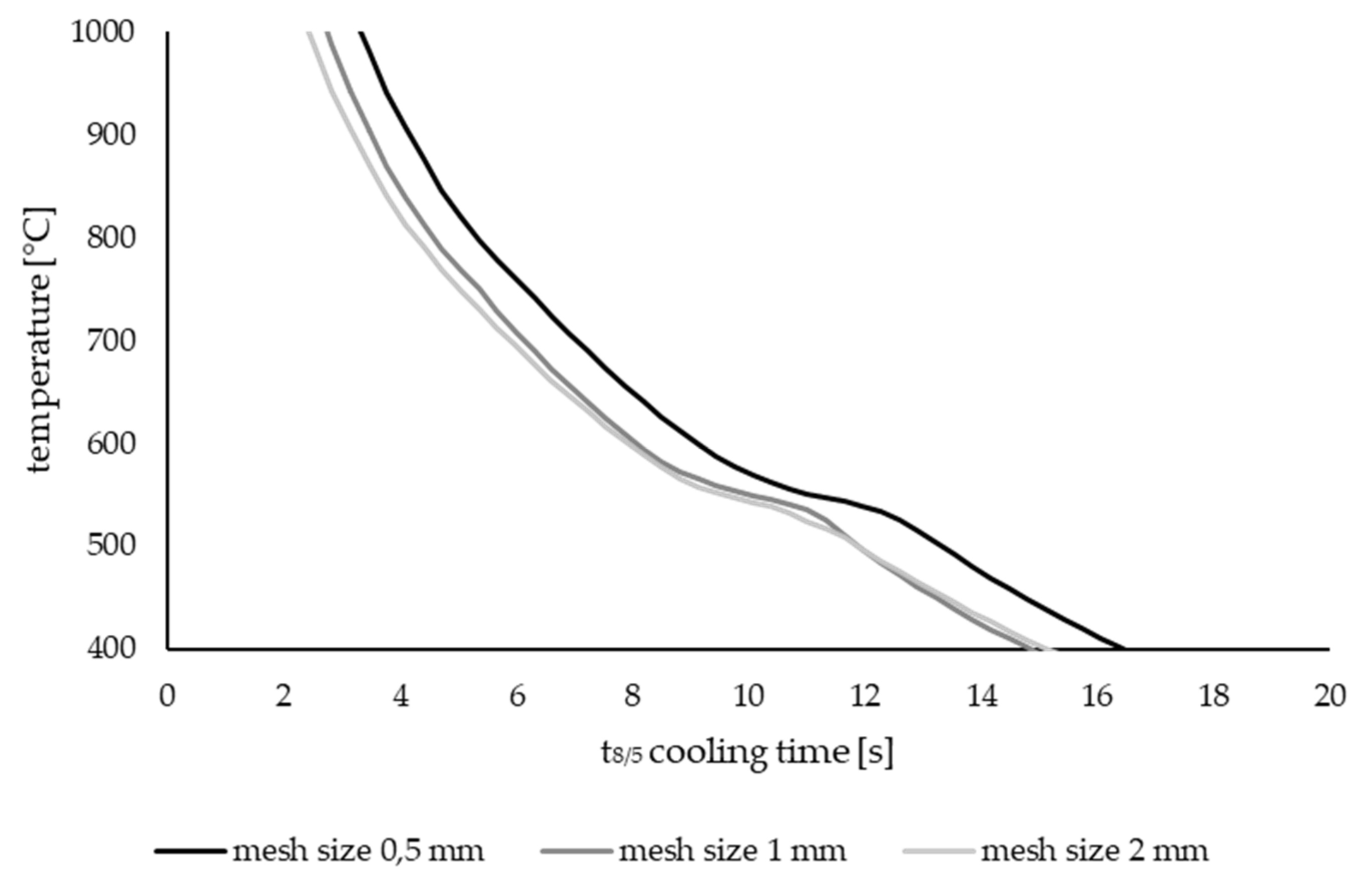
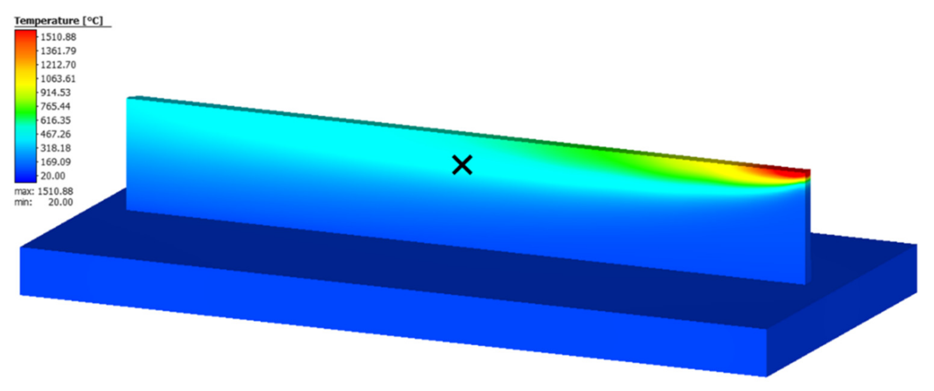
3.2. Numerical Simulation

Figure 12 demonstrates the temperature field of the wall structure at the last calculation step of the 25th welding layer. Figure 13 shows the time temperature cycle for the 20th layer. In the state of the art, it was demonstrated that it is possible to recreate the thermal cycles of DED-Arc within the numerical simulation with relative errors below 20%, which was considered acceptable by the authors [56]. The time–temperature diagrams show a similar pattern to that in the state of the art [33,35,37,38,56]. The t_8/5 cooling time of the experimental test was 15.94 s and the welding simulation took 16.38 s to pass through the temperature interval between 800 °C and 500 °C for the last time. This is a difference of 2.69%, which is a fairly accurate result for a partly validated numerical simulation with an experimental sample size of one part.

Figure 14 and Figure 15 demonstrate the simulated temperature field and time–temperature profile of a known sample just used for validation, which was not used to generate the regression equations. For this simulation, only the welding heat source size, the process parameters and the wall thickness were changed to match the new parameter set. The t_8/5 cooling time in the numerical simulation took 30.15 s to pass through the temperature interval between 800 °C and 500 °C, which is only 0.09 s above the experimentally measured t_8/5 cooling time. The results of the time–temperature diagram are similar to the state of the art [33,35,37,38,56].

3.3. Validation of Regression Equation

The regression equations, which are found in Figure 10, were used to calculate the mechanical properties of the numerically determined t_8/5 cooling time for the energy input per unit length 8 kJ/cm of sample with a wall thickness of 9 mm. The experimental calculated values and the deviation between them can be seen in

Table 4. Comparison of measured and calculated t_8/5 cooling times and mechanical properties.

Sample with Energy Input per Unit Length 8 kJ	t8/5	Hardness HV1	Tensile Strength	Yield Strength	Elongation at Break
Experimental values	30.06 s	166.1	507.6 MPa	377.3 MPa	35.3%
Predicted values	30.15 s	168.1	502.1 MPa	380.1 MPa	34.4%
Deviation [%]	0.3	1.2	1.1	0.7	2.6

. The deviation in hardness and tensile strength is just above 1%; for the yield strength it is below 1%. The elongation at break shows the highest difference with a deviation of 2.6%. As shown, the calculated values are not very different from the reference sample. In

Table 5. Coefficient of determination and standard error for the regression equations.

	R²	Standard Error
Hardness	0.6520	8.60
Tensile strength	0.8445	17.74
Yield strength	0.8752	21.37
Elongation at break	0.5192	1.49

the coefficient of determination (R²) and the corresponding standard error are given. The R² value is a measure of how well observed outcomes are replicated by the model. The R² values vary between 51.9% and 87.5%. The standard error is dependent on the measured value. Compared to the average values in each regression the average distance of the data points from the regression curve is 8.6 (4.8%) for the hardness, 17.74 (3.3%) for the tensile strength, 21.37 (4.9%) for the yield strength and 1.49 (4.5%) for the elongation at break. These are low deviations considering that relative errors below 20% are considered acceptable for a numerical simulation [56].

4. Conclusions

This study has shown that a lower t_8/5 cooling time is beneficial to the mechanical properties of additively manufactured structures made of G4Si1. In DED-Arc it is not always possible to ensure the same cooling times for the whole additively manufactured structure due to geometrical constraints, such as a irregular wall thickness, curves, edges and cross points in a three-dimensional freeform shape. Thus, it is key to approximate the mechanical properties based on different t_8/5 cooling times; moreover, this enables machine learning algorithms to obtain a much larger amount of data due to the generation of synthetic data. Therefore, the underlying regression equations of the relation between mechanical property and t_8/5 cooling time are needed. The hardness and t_8/5 cooling times in the state of the art demonstrate the logarithmic relation between them. The results found in this research can be concluded with the following statements:

•

The hardness, tensile strength, yield strength and elongation at break show a logarithmic relation with the t_8/5 cooling times (Figure 9 and Figure 10).

•

Therefore, it is possible to calculate values between the given data points by using the regression equations Figure 9 and Figure 10.

•

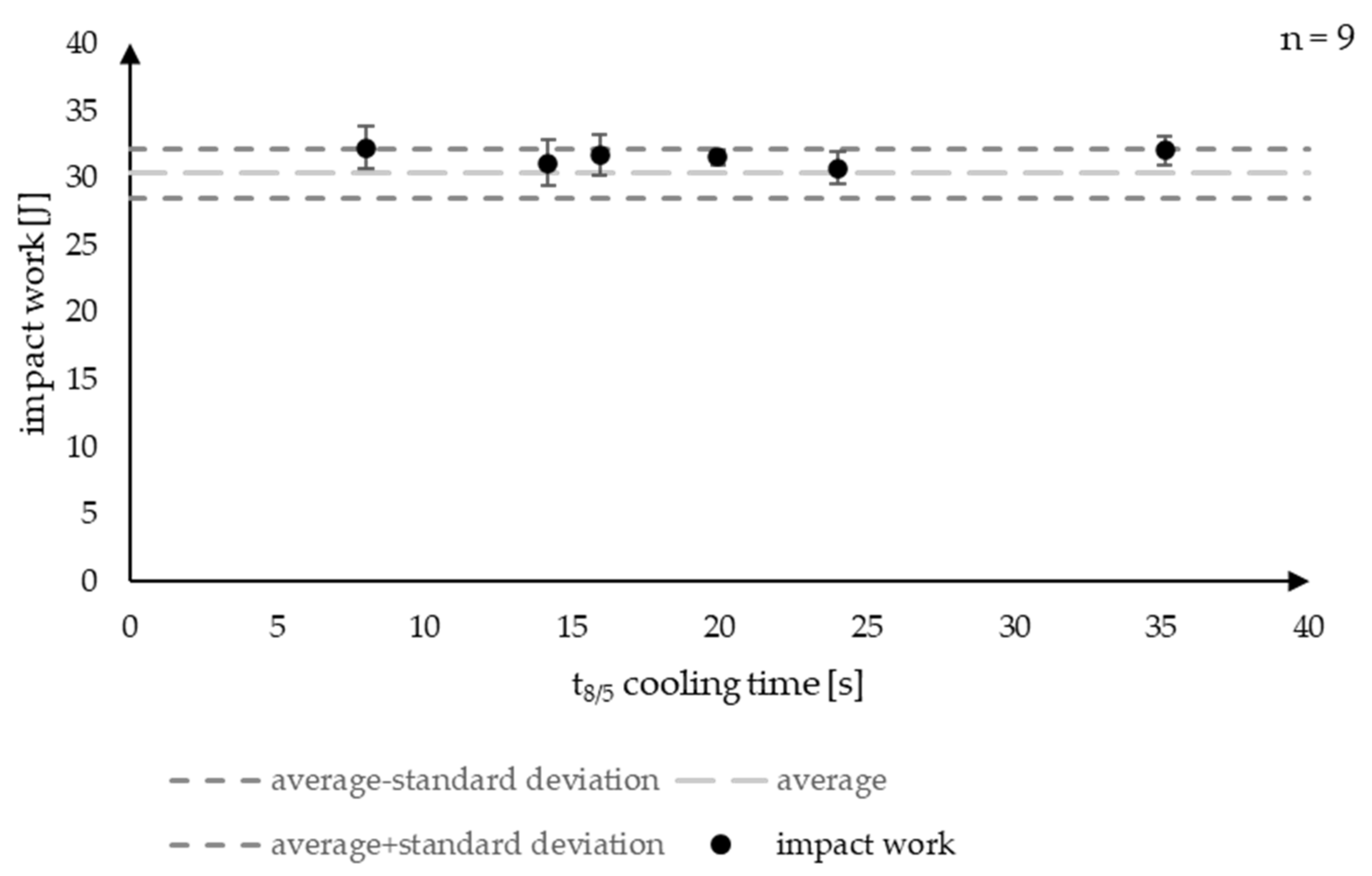
The impact work was the only mechanical property tested in this research with no obvious relation to the t_8/5 cooling times (Figure 11).

•

The numerical simulation was a suitable tool to calculate the t_8/5 cooling time (Figure 13) for a tested parameter set (Figure 15) with a deviation of only 0.3% (Table 4).

•

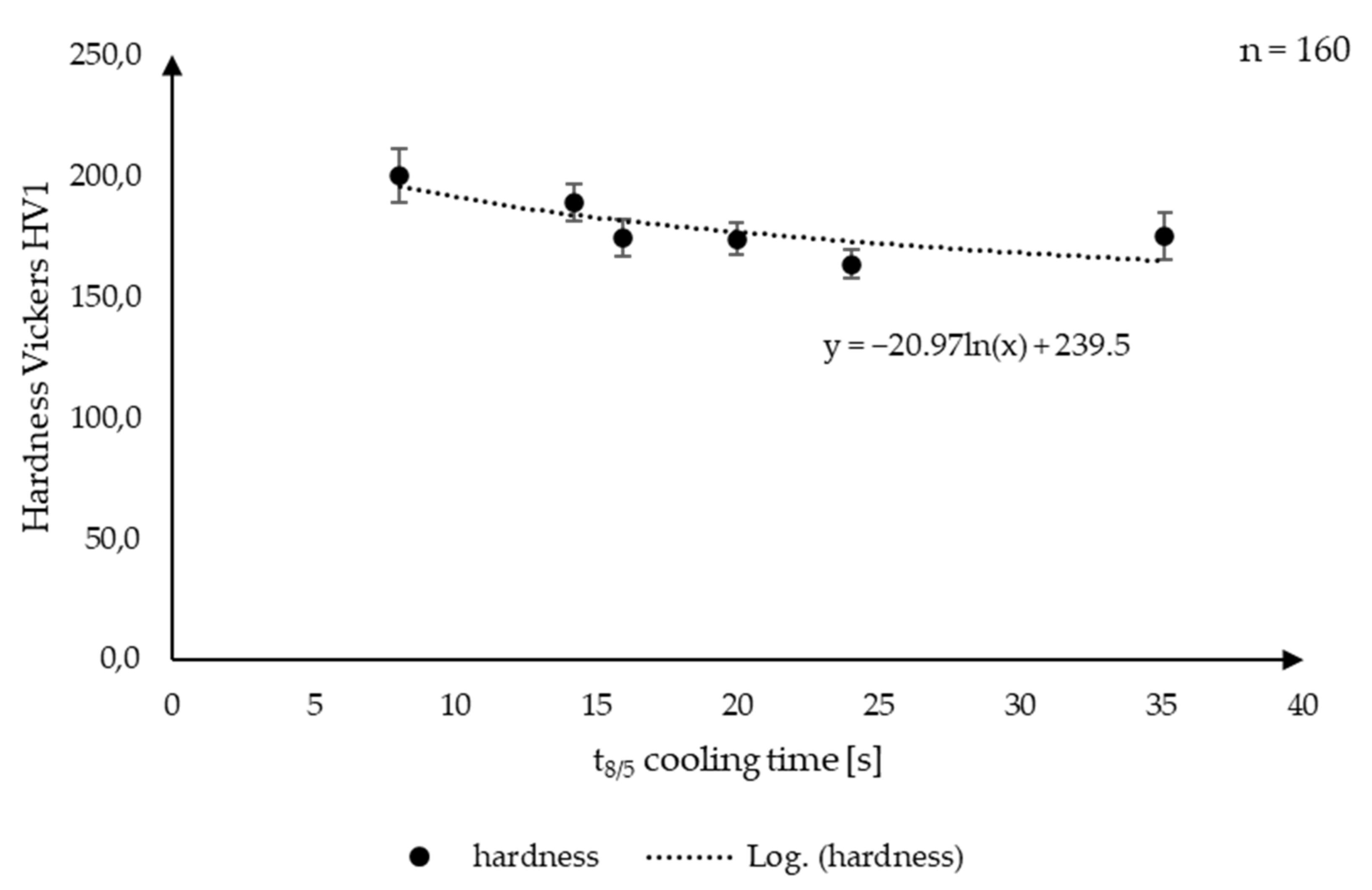
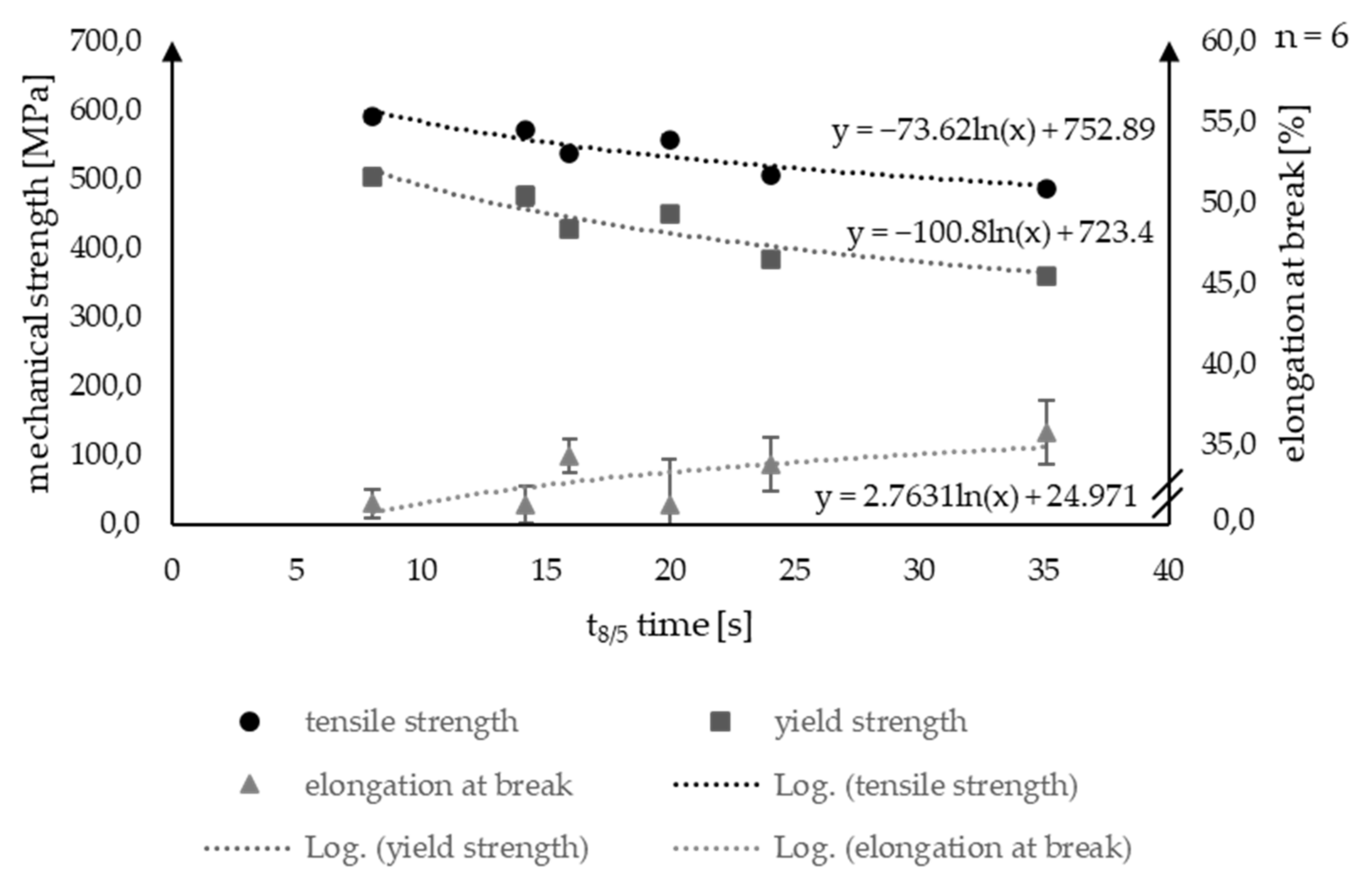
The regression equations have proven to have a high prediction accuracy, with only small deviations from the measured values of 1.2% for the hardness, 1.1% for the tensile strength, 0.7% for the yield strength and 2.6% for the elongation at break (Table 4).

Yet, a completely validated simulation model for different parameter sets would provide even more accurate results. Therefore, a combination of the numerical simulation and the experimentally determined regression equations can be used as a tool for the data augmentation. As the given parameter sets were limited in this research, a broader study would generate more accurate regression equations. In future, a more complete data set should be used as the basis for regression equations. Parameter sets with higher cooling times than 35.1 s and lower than 8 s would be needed.

References

1. Wohlers Report 2019 Details Striking Range of Developments in Am Worldwide. Available online: https://www.3dprintingmedia.network/wohlers-report-2019-details-striking-range-of-developments-in-am-worldwide/ (accessed on 16 June 2021).
2. Karunakaran, K.P.; Bernard, A.; Suryakumar, S.; Dembinski, L.; Taillandier, G. Rapid manufacturing of metallic objects. Rapid Prototyp. J. 2012, 18, 264–280. [Google Scholar] [CrossRef]
3. Hildebrand, J. Additive Fertigung von temperierten Großwerkzeugen mittels Lichtbogen-und Diffusionsschweißtechnik. In Rapid.Tech + FabCon 3.D: International Trade Show + Conference for Additive Manufacturing: Proceedings of the 15th Rapid Tech Conference, Erfurt, Germany, 5–7 June 2018; Kynast, M., Eichmann, M., Witt, G., Eds.; Hanser: München, Germany, 2018; pp. 29–44. ISBN 3446458115. [Google Scholar]
4. Jahn, S.; Gemse, F.; Broich, U.; Saendig, S. Efficient Diffusion Bonding of Large Scale Parts. MSF 2016, 838–839, 500–505. [Google Scholar] [CrossRef]
5. Karunakaran, K.P.; Suryakumar, S.; Pushpa, V.; Akula, S. Low cost integration of additive and subtractive processes for hybrid layered manufacturing. Robot. Comput. Integr. Manuf. 2010, 26, 490–499. [Google Scholar] [CrossRef]
6. Wu, B.; Pan, Z.; Ding, D.; Cuiuri, D.; Li, H.; Xu, J.; Norrish, J. A review of the wire arc additive manufacturing of metals: Properties, defects and quality improvement. J. Manuf. Process. 2018, 35, 127–139. [Google Scholar] [CrossRef]
7. Williams, S.W.; Martina, F.; Addison, A.C.; Ding, J.; Pardal, G.; Colegrove, P. Wire + Arc Additive Manufacturing. Mater. Sci. Technol. 2016, 32, 641–647. [Google Scholar] [CrossRef] [Green Version]
8. Ding, D.; Pan, Z.; Cuiuri, D.; Li, H. Wire-feed additive manufacturing of metal components: Technologies, developments and future interests. Int. J. Adv. Manuf. Technol. 2015, 81, 465–481. [Google Scholar] [CrossRef]
9. Candel-Ruiz, A.; Kaufmann, S.; Muellerschoen, O. Strategies for high deposition rate additive manufacturing by laser metal deposition. Lasers Manuf. Conf. 2015, 2015, 584. [Google Scholar]
10. Bergmann, J.P.; Henckell, P.; Ali, Y.; Hildebrand, J.; Reimann, J. Grundlegende Wissenschaftliche Konzepterstellung zu Bestehenden Herausforderungen und Perspektiven für die Additive Fertigung Mit Lichtbogen: Studie im Auftrag der Forschungsvereinigung Schweißen und Verwandte Verfahren e.V. des DVS; DVS Media: Düsseldorf, Germany, 2018; ISBN 978-3-96144-038-2. [Google Scholar]
11. Cunningham, C.R.; Flynn, J.M.; Shokrani, A.; Dhokia, V.; Newman, S.T. Invited review article: Strategies and processes for high quality wire arc additive manufacturing. Addit. Manuf. 2018, 22, 672–686. [Google Scholar] [CrossRef]
12. Asala, G.; Khan, A.K.; Andersson, J.; Ojo, O.A. Microstructural Analyses of ATI 718Plus® Produced by Wire-ARC Additive Manufacturing Process. Metall. Mater. Trans. A 2017, 48, 4211–4228. [Google Scholar] [CrossRef] [Green Version]
13. Dhinakaran, V.; Ajith, J.; Fathima Yasin Fahmidha, A.; Jagadeesha, T.; Sathish, T.; Stalin, B. Wire Arc Additive Manufacturing (WAAM) process of nickel based superalloys—A review. Mater. Today Proc. 2020, 21, 920–925. [Google Scholar] [CrossRef]
14. Mehnen, J.; Ding, J.; Lockett, H.; Kazanas, P. Design study for wire and arc additive manufacture. Int. J. Prod. Dev. 2014, 19, 2. [Google Scholar] [CrossRef]
15. Bermingham, M.J.; Nicastro, L.; Kent, D.; Chen, Y.; Dargusch, M.S. Optimising the mechanical properties of Ti-6Al-4V components produced by wire + arc additive manufacturing with post-process heat treatments. J. Alloy. Compd. 2018, 753, 247–255. [Google Scholar] [CrossRef]
16. Lu, X.; Zhou, Y.F.; Xing, X.L.; Shao, L.Y.; Yang, Q.X.; Gao, S.Y. Open-source wire and arc additive manufacturing system: Formability, microstructures, and mechanical properties. Int. J. Adv. Manuf. Technol. 2017, 93, 2145–2154. [Google Scholar] [CrossRef]
17. Reimann, J.; Hildebrand, J.; Bergmann, J.P. 3D-Weld-3D Gedruckte Knotenpunkte aus Stahllegierungen für Bionische Tragstrukturen; Fraunhofer IRB Verlag: Stuttgart, Germany, 2020; ISBN 9783738804720. [Google Scholar]
18. Reimann, J.; Henckell, P.; Ali, Y.; Hammer, S.; Rauch, A.; Hildebrand, J.; Bergmann, J.P. Production of Topology-optimised Structural Nodes Using Arc-based, Additive Manufacturing with GMAW Welding Process. J. Civ. Eng. Constr. 2021, 10, 101–107. [Google Scholar] [CrossRef]
19. Abdelwahab, M.; Tsavdaridis, K.D. Optimised 3D-Printed Metallic Node-Connections for Reticulated Structures. In Proceedings of the 9th International Conference on Steel and Aluminium Structures, Bradford, UK, 3–5 July 2019. [Google Scholar] [CrossRef] [Green Version]
20. Galjaard, S.; Hofman, S.; Ren, S. New Opportunities to Optimize Structural Designs in Metal by Using Additive Manufacturing. In Advances in Architectural Geometry 2014; Block, P., Knippers, J., Mitra, N.J., Wang, W., Eds.; Springer: Cham, Switzerland; New York, NY, USA, 2015; pp. 79–93. ISBN 978-3-319-11417-0. [Google Scholar]
21. Feucht, T.; Lange, J.; Waldschmitt, B.; Schudlich, A.-K.; Klein, M.; Oechsner, M. Welding Process for the Additive Manufacturing of Cantilevered Components with the WAAM. In Advanced Joining Processes; da Silva, L.F.M., Martins, P.A.F., El-Zein, M.S., Eds.; Springer: Singapore, 2020; pp. 67–78. ISBN 978-981-15-2956-6. [Google Scholar]
22. Ghaffari, M.; Vahedi Nemani, A.; Rafieazad, M.; Nasiri, A. Effect of Solidification Defects and HAZ Softening on the Anisotropic Mechanical Properties of a Wire Arc Additive-Manufactured Low-Carbon Low-Alloy Steel Part. JOM 2019, 71, 4215–4224. [Google Scholar] [CrossRef]
23. Müller, J.; Grabowski, M.; Müller, C.; Hensel, J.; Unglaub, J.; Thiele, K.; Kloft, H.; Dilger, K. Design and Parameter Identification of Wire and Arc Additively Manufactured (WAAM) Steel Bars for Use in Construction. Metals 2019, 9, 725. [Google Scholar] [CrossRef] [Green Version]
24. Rafieazad, M.; Ghaffari, M.; Vahedi Nemani, A.; Nasiri, A. Microstructural evolution and mechanical properties of a low-carbon low-alloy steel produced by wire arc additive manufacturing. Int. J. Adv. Manuf. Technol. 2019, 105, 2121–2134. [Google Scholar] [CrossRef]
25. Gordon, J.; Hochhalter, J.; Haden, C.; Harlow, D.G. Enhancement in fatigue performance of metastable austenitic stainless steel through directed energy deposition additive manufacturing. Mater. Des. 2019, 168, 107630. [Google Scholar] [CrossRef]
26. Wu, W.; Xue, J.; Wang, L.; Zhang, Z.; Hu, Y.; Dong, C. Forming Process, Microstructure, and Mechanical Properties of Thin-Walled 316L Stainless Steel Using Speed-Cold-Welding Additive Manufacturing. Metals 2019, 9, 109. [Google Scholar] [CrossRef] [Green Version]
27. Ali, Y.; Henckell, P.; Hildebrand, J.; Reimann, J.; Bergmann, J.P.; Barnikol-Oettler, S. Wire arc additive manufacturing of hot work tool steel with CMT process. J. Mater. Process. Technol. 2019, 269, 109–116. [Google Scholar] [CrossRef]
28. Gierth, M.; Henckell, P.; Ali, Y.; Scholl, J.; Bergmann, J.P. Wire Arc Additive Manufacturing (WAAM) of Aluminum Alloy AlMg5Mn with Energy-Reduced Gas Metal Arc Welding (GMAW). Materials 2020, 13, 2671. [Google Scholar] [CrossRef] [PubMed]
29. Gu, J.; Gao, M.; Yang, S.; Bai, J.; Zhai, Y.; Ding, J. Microstructure, defects, and mechanical properties of wire + arc additively manufactured Al Cu4.3-Mg1.5 alloy. Mater. Des. 2020, 186, 108357. [Google Scholar] [CrossRef]
30. Geng, H.; Li, J.; Xiong, J.; Lin, X. Optimisation of interpass temperature and heat input for wire and arc additive manufacturing 5A06 aluminium alloy. Sci. Technol. Weld. Join. 2017, 22, 472–483. [Google Scholar] [CrossRef]
31. Zhao, Y.; Jia, Y.; Chen, S.; Shi, J.; Li, F. Process planning strategy for wire-arc additive manufacturing: Thermal behavior considerations. Addit. Manuf. 2020, 32, 100935. [Google Scholar] [CrossRef]
32. Montevecchi, F.; Venturini, G.; Scippa, A.; Campatelli, G. Finite Element Modelling of Wire-arc-additive-manufacturing Process. Procedia CIRP 2016, 55, 109–114. [Google Scholar] [CrossRef] [Green Version]
33. Ding, J.; Colegrove, P.; Mehnen, J.; Ganguly, S.; Sequeira Almeida, P.M.; Wang, F.; Williams, S. Thermo-mechanical analysis of Wire and Arc Additive Layer Manufacturing process on large multi-layer parts. Comput. Mater. Sci. 2011, 50, 3315–3322. [Google Scholar] [CrossRef] [Green Version]
34. Graf, M.; Pradjadhiana, K.P.; Hälsig, A.; Manurung, Y.H.P.; Awiszus, B. Numerical simulation of metallic wire arc additive manufacturing (WAAM). In Proceedings of the 21st International ESAFORM Conference on Material Forming: ESAFORM 2018, Palermo, Italy, 23–25 April 2018; p. 140010. [Google Scholar]
35. Graf, M.; Hälsig, A.; Höfer, K.; Awiszus, B.; Mayr, P. Thermo-Mechanical Modelling of Wire-Arc Additive Manufacturing (WAAM) of Semi-Finished Products. Metals 2018, 8, 1009. [Google Scholar] [CrossRef] [Green Version]
36. Hu, Z.; Qin, X.; Shao, T. Welding Thermal Simulation and Metallurgical Characteristics Analysis in WAAM for 5CrNiMo Hot Forging Die Remanufacturing. Procedia Eng. 2017, 207, 2203–2208. [Google Scholar] [CrossRef]
37. Montevecchi, F.; Venturini, G.; Grossi, N.; Scippa, A.; Campatelli, G. Heat accumulation prevention in Wire-Arc-Additive-Manufacturing using air jet impingement. Manuf. Lett. 2018, 17, 14–18. [Google Scholar] [CrossRef]
38. Ding, J. Thermo-Mechanical Analysis of Wire and Arc Additive Manufacturing Process; Cranfield University: Cranfield, UK, 2012. [Google Scholar]
39. Perez, L.; Wang, J. The Effectiveness of Data Augmentation in Image Classification using Deep Learning. arXiv 2017, arXiv:1712.04621. [Google Scholar]
40. Fawaz, H.I.; Forestier, G.; Weber, J.; Idoumghar, L.; Muller, P.-A. Deep Learning for Time Series Classification: A review No. 4. Data Min. Knowl. Discov. 2019, 33, 917–963. [Google Scholar] [CrossRef] [Green Version]
41. Wen, Q.; Sun, L.; Yang, F.; Song, X.; Gao, J.; Wang, X.; Xu, H. Time Series Data Augmentation for Deep Learning: A Survey. arXiv 2020, arXiv:2002.12478. [Google Scholar]
42. Jäckel, M.; Falk, T.; Georgi, J.; Drossel, W.-G. Gathering of Process Data through Numerical Simulation for the Application of Machine Learning Prognosis Algorithms. Procedia Manuf. 2020, 47, 608–614. [Google Scholar] [CrossRef]
43. Zhang, Z.; Wen, G.; Chen, S. Weld image deep learning-based on-line defects detection using convolutional neural networks for Al alloy in robotic arc welding. J. Manuf. Process. 2019, 45, 208–216. [Google Scholar] [CrossRef]
44. Pu, X.; Zhang, C.; Li, S.; Deng, D. Simulating welding residual stress and deformation in a multi-pass butt-welded joint considering balance between computing time and prediction accuracy. Int. J. Adv. Manuf. Technol. 2017, 93, 2215–2226. [Google Scholar] [CrossRef]
45. Rikken, M.; Pijpers, R.; Slot, H.; Maljaars, J. A combined experimental and numerical examination of welding residual stresses. J. Mater. Process. Technol. 2018, 261, 98–106. [Google Scholar] [CrossRef]
46. Salzgitter, F.G. S355J2+N: Unlegierte Baustähle. Available online: https://www.salzgitter-flachstahl.de/fileadmin/mediadb/szfg/informationsmaterial/produktinformationen/warmgewalzte_produkte/deu/S355J2_N.pdf (accessed on 17 July 2021).
47. Westfälische, D.G. Schweisstechnik: High Quality Welding Wire. Technisches Handbuch. Available online: https://www.wdi.de/fileadmin/user_upload/WDI_SFHandbuch_3_Edition_screen.pdf (accessed on 12 July 2021).
48. DIN EN 1011-2:2001-05, Schweißen_- Empfehlungen zum Schweißen Metallischer Werkstoffe_- Teil_2: Lichtbogenschweißen von Ferritischen Stählen. In Deutsche Fassung EN_1011-2:2001; Beuth Verlag GmbH: Berlin, Germany, 2001.
49. Stahlinstitut, V. Weldable Non-Alloy and Low-Alloy Steels: Recommendations for Processing, in Particular for Fusion Welding, SEW 088:2017-10; Stahleisen: Düsseldorf, Germany, 2017; (SEW088). [Google Scholar]
50. Henckell, P.; Gierth, M.; Ali, Y.; Reimann, J.; Bergmann, J.P. Reduction of Energy Input in Wire Arc Additive Manufacturing (WAAM) with Gas Metal Arc Welding (GMAW). Materials 2020, 13, 2491. [Google Scholar] [CrossRef] [PubMed]
51. Seyffarth, P.; Meyer, B.; Scharff, A. Großer Atlas Schweiß-ZTU-Schaubilder, 2., Aktualisierte und Erweiterte Auflage; DVS Media GmbH: Dusseldorf, Germany, 2018; ISBN 3961440107. [Google Scholar]
52. Schulze, G. Die Metallurgie des Schweissens: Eisenwerkstoffe-Nichteisenmetallische Werkstoffe, 4., neu Bearbeitete Auflage; Springer: Berlin/Heidelberg, Germany; New York, NY, USA, 2010; ISBN 3642031838. [Google Scholar]
53. Shassere, B.; Nycz, A.; Noakes, M.; Masuo, C.; Sridharan, N. Correlation of Microstructure and Mechanical Properties of Metal Big Area Additive Manufacturing. Appl. Sci. 2019, 9, 787. [Google Scholar] [CrossRef] [Green Version]
54. Dirisu, P.; Ganguly, S.; Mehmanparast, A.; Martina, F.; Williams, S. Analysis of fracture toughness properties of wire + arc additive manufactured high strength low alloy structural steel components. Mater. Sci. Eng. A 2019, 765, 138285. [Google Scholar] [CrossRef]
55. Aldalur, E.; Veiga, F.; Suárez, A.; Bilbao, J.; Lamikiz, A. High deposition wire arc additive manufacturing of mild steel: Strategies and heat input effect on microstructure and mechanical properties. J. Manuf. Process. 2020, 58, 615–626. [Google Scholar] [CrossRef]
56. Prajadhiama, K.P.; Manurung, Y.H.P.; Minggu, Z.; Pengadau, F.H.S.; Graf, M.; Haelsig, A.; Adams, T.-E.; Choo, H.L. Development of Bead Modelling for Distortion Analysis Induced by Wire Arc Additive Manufacturing using FEM and Experiment. MATEC Web Conf. 2019, 269, 5003. [Google Scholar] [CrossRef]
Figure 1. Process chain of additive manufacturing using DED-Arc according to [10].
Applsci 11 07075 g001
Figure 2. Experimental setup.
Applsci 11 07075 g002
Figure 3. Welding TTT-diagram of a chemical comparable material as G4Si1 [51] (translated).
Applsci 11 07075 g003
Figure 4. Layout of samples for mechanical testing of an additively manufactured wall structure.
Applsci 11 07075 g004
Figure 5. Testing equipment for mechanical properties; left: universal testing machine Zwick 1455, middle: WPM PSd 300/150, right: Struers DuraScan 70.
Applsci 11 07075 g005
Figure 6. Mesh convergence for mesh sizes 0.5 mm, 1.0 mm and 2 mm.
Applsci 11 07075 g006
Figure 7. Samples of additively manufactured wall structures 4 kJ/cm: (1) single weld track; (2) two adjacent weld tracks; (3) three adjacent weld tracks.
Applsci 11 07075 g007
Figure 8. Hardness as a function of t8/5 cooling time (values for hardness and t8/5 cooling time according to the welding TTT diagram shown in Figure 3).
Applsci 11 07075 g008
Figure 9. Hardness as a function of t8/5 cooling time from measured data.
Applsci 11 07075 g009
Figure 10. Tensile, yield strength and elongation at break as a function of t8/5 cooling time from measured data.
Applsci 11 07075 g010
Figure 11. Charpy impact test over t8/5 cooling time from measured data.
Applsci 11 07075 g011
Figure 12. Temperature field in the welding simulation for wall structure (length 300 mm) and energy input per unit length 4 kJ/cm with layer 25.
Applsci 11 07075 g012
Figure 13. Time–temperature cycle for point x in the welding simulation for wall structure (length 300 mm) and energy input per unit length 4 kJ/cm with layer 25.
Applsci 11 07075 g013
Figure 14. Temperature field in the welding simulation for wall structure (length 300 mm) and energy input per unit length 8 kJ/cm with layer 25.
Applsci 11 07075 g014
Figure 15. Time-temperature cycle in the welding simulation for wall structure (length 300 mm) and energy input per unit length 8 kJ/cm with layer 25.
Applsci 11 07075 g015