Article

SOPRENE: Assessment of the Spanish Armada’s Predictive Maintenance Tool for Naval Assets

by
David Fernández-Barrero
1,
Oscar Fontenla-Romero
2,
Francisco Lamas-López
3,
David Novoa-Paradela
2,
María D. R-Moreno
1 and
David Sanz
4,*
1
Departamento de Automática, Universidad de Alcalá, 28801 Madrid, Spain
2
Centro de Investigación TIC (CITIC), Universidade da Coruña, 15008 A Coruña, Spain
3
CESADAR-CENTRAL, Armada Española, 30201 Cartagena, Spain
4
INDRA, 28108 Madrid, Spain
*
Author to whom correspondence should be addressed.
Appl. Sci. 2021, 11(16), 7322; https://doi.org/10.3390/app11167322
Submission received: 15 July 2021 / Revised: 26 July 2021 / Accepted: 28 July 2021 / Published: 9 August 2021
(This article belongs to the Special Issue Overcoming the Obstacles to Predictive Maintenance)

Abstract

:
Predictive maintenance has lately proved to be a useful tool for optimizing costs, performance and systems availability. Furthermore, the greater and more complex the system, the higher the benefit but also the less applied: Architectural, computational and complexity limitations have historically ballasted the adoption of predictive maintenance on the biggest systems. This has been especially true in military systems where the security and criticality of the operations do not accept uncertainty. This paper describes the work conducted in addressing these challenges, aiming to evaluate its applicability in a real scenario: It presents a specific design and development for an actual big and diverse ecosystem of equipment, proposing an semi-unsupervised predictive maintenance system. In addition, it depicts the solution deployment, test and technological adoption of real-world military operative environments and validates the applicability.

1. Introduction

Depending on the field, forecasting capabilities can be translated into different advantages such as economic benefits in stock markets or business development; the incremental increase in the capabilities of saving a life or improving the quality of life in medicine; operational superiority in defense and security. In maintenance, prediction implies all the above.
On the one hand, scheduled maintenance costs represent a significant part of total operating costs in industrial environments. In the metallurgical industry, for example, the storage, provisioning and reparation costs can imply 15–60% of total production costs [1]. Moreover, one-third of this money invested in maintenance management is wasted as a result of unnecessary or incorrect activities. Furthermore, unexpected maintenance has a direct translation on the availability of services or capabilities, which may have an impact over the security, brand image, third parties confidence, etc.
One of the most common maintenance strategies is preventive maintenance, which is based on regular inspections of the machines in a planned, programmed and controlled manner, in order to anticipate functional failures. It consists of preventing the deterioration suffered in an equipment due to different variables, such as normal use, the weather or failures of an accessory that do not affect the main function, while the activities are carried out in anticipating that the equipment presents major failures. Predictive maintenance (PdM) is one of the most widespread strategies worldwide and is based on the periodic measurement of the variables that determine the condition of the equipment while it is operating. Specialized techniques and tools are used for its execution, which prematurely detect failures and develop actions to correct them. Predictive maintenance uses data analysis techniques that allow forecasting possible errors or defects in the machinery at its initial stages in order to avoid these failures becoming more serious and so that its parts can be replaced in advance. As benefits of predictive versus preventive maintenance, the following can be highlighted: reduction in the number of interventions on the equipment, reduction in downtime to perform maintenance tasks and costs minimization in maintenance tasks. In this sense, the main advantage of predictive maintenance is its ability to anticipate the future state of the monitored system and, therefore, extend the useful life of its assets, as demonstrated in various industrial applications such as electrical equipment maintenance [2,3].
The impossibility to efficiently deal with large and continuous flows of data in the past made actual predictive maintenance impossible in the industry. Techniques based on statistical trends (e.g., mean time between failures) had to be used to improve the maintenance procedures. However, today’s current computing capacity and advanced Machine Learning (ML) techniques render it possible to perform real-time monitoring of the system’s mechanical condition to predict when components will fail [1,4]. In this sense, predictive maintenance is currently understood as preventive maintenance [5] conditioned to the current state of the system and to the predictions of the future state made from operation history.
Significant results have been obtained on the PdM area in the recent years. However, most of the developments come from equipment that is either not quite complex (i.e., IoT, smart sensors, etc.) [6] or quite specific and invariant (i.e., wind or gas turbines) [7,8]. The application of PdM techniques over real, productive, big and complex systems with changing conditions with multitudes of options and configurations are still a challenge. Furthermore, although some industries have already dealt with it—even including tentative PdM processes in some of their value chains [9]—predictive maintenance has been rarely been considered in the defense industry or the military: The robustness, reliability and security requirements are very strict and defiant and a reduced number of works have been carried out (publicly) [10].
This research work addresses both challenges: It presents the design and implementation of predictive maintenance distributed architecture for big, complex and heterogeneous pieces of military equipment. Furthermore, the concept has been validated over warships’ systems, where some traditional maintenance work have been performed [11], but, to author’s knowledge, no predictive capabilities have been applied.
In order to present all this information coherently, the paper is structured as follows: Section 2 presents the goals, challenges and context of the research work performed in the SOPRENE project. Then, Section 3 analyzes the main works performed in the predictive maintenance field and, subsequently, aligns with PdM works. Section 4 describes the unified architecture designed to deal with big, scalable and heterogeneous systems, while the results obtained from its validation are described in Section 5. Finally, the conclusions are outlined in Section 6.

2. Problem Statement

Aligned with the PM challenges and goals stated in Section 1, the Spanish navy (also called Spanish Armada, SA) together with the General Directorate of Armament and Material (DGAM) of the Spanish Ministry of Defense planned the SOPRENE R&D program in 2017.
The main objective of SOPRENE was to provide both short and long term predictive capabilities for the SN equipment [12]. The solution should deliver the forthcoming failures, breaking them down according to their class and probability of occurrence and overcoming robustness, efficiency and versatility challenges associated with military PdM development. Moreover, the solution should be integrated into the logistical and operational decision processes of the navy.
According to this, the project started in 2018 and has successfully concluded in the beginning of 2021. It has been leaded by Indra in collaboration with several Spanish universities that have delivered a scalable, accurate and fully functional demonstrator to the Spanish Armada.
This demonstrator has been developed according to the following.

2.1. Equipment Selection and Scalability

One of the SOPRENE’s main goals is to guarantee the applicability of the solution for the diverse naval platform equipment and assets of the Spanish Navy. Thus, the scalability of the solution—both vertical and horizontal—was a hard requirement to be proven by the demonstrator. In this sense, different systems of different ships of different classes were selected for the validation: Four BAM class vessels (Maritime Action Vessels) and five F-100 class frigates were chosen by selecting the diesel propellants and power generation equipment for them, respectively [13].
Likewise, the solution should be able to detect and diagnose failures never experienced by any ship of the Spanish fleet. In order for this to be possible, the discretization of the possible failure modes should rely on theoretical working information covered by a failure mode, effects and criticality analysis (FMECA). The information provided by the FMECA should be aligned with the data provided from sensors and alarms and adapted to the application of ML-based prediction algorithms (i.e., numerical, boolean or categorical registers).

2.2. Data Availability and Management

The management of SN data, which includes tens of thousands variables of several dozens of systems, is carried out by the Centre for Data Supervision and Analysis of the Spanish Armada (CESADAR). It collects and stores the operational information of each of their vessels and pieces of equipment, aligning their different acquisition frequencies and data type. This information is available from 2011 onward and includes data from the equipment control and operation sensors (IPMS Navantia system); specific information of vibrations collected by the condition-based maintenance software (CBM); and data from fluid analysis laboratory (PAESA system). Unfortunately, the information related to maintenance and failures, although available, had a different sift and could not provide a proper labeling.
This information is stored and structured within the CESADAR datalake. The SOPRENE program shall use a full functional big data platform to access the data, process it and transfer the results. Data from 2011 to 2016 would be used to train the system and evaluate the normality. This temporal range assures the availability of all the operational modes and weather conditions. Finally, data from the years from 2016 to 2019 would be used to evaluate the performance and suitability of the solution.

3. State of the Art

This section provides a brief review of the main approaches that have been recently used for PdM.
Ran et al. [14] provided a categorization based on the optimization criteria. In this direction, He et al. [15] presented an approach that minimizes the cost of the Remaining Useful Life (RUL) of the system, although they showed that it is also possible to define an ad hoc cost model. Other multi-objective optimization works seek to optimize multiple metrics simultaneously in order to achieve a better balance between objectives. In addition to the aforementioned, they employ metrics such as risk, security or viability. Generally, it is impossible to obtain optimal values for all objectives at the same time, which is why a wide variety of multi-objective models have been developed [16,17,18]. Other research define metrics to maximize the reliability and availability of the system. For example, Song et al. defined the probability of a system to be in a normal operating state in a given time interval [19] while Gravette and Barker [20] defined the probability that the system is operational.
Other works focus on the type of approach used to solve the problem. Some use expert knowledge and deductive reasoning processes. For example, there are works based on ontologies [21], on rules [22] or on models that try to link the physical processes of a system with mathematical models, such as Gaussian models [23], linear systems models [24] or Markov models [25].
In the arena of ML techniques, Artificial Neuronal Networks (ANN) [26] and decision trees [27] (including the Random Forest algorithm [28]) have been used, as well as Support Vector Machines (SVM) in terms of both supervised [29] and unsupervised [30] learning. Finally, the k-Nearest Neighbor Technique (k-NN) is one of the most common for fault classification [31], for prediction of useful life time (RUL) [32] and early detection [33]. One of the most used Deep Learning (DL) techniques is the Autoencoder Neural Networks, for which its output layer seeks to reproduce the data presented in its input layer after having gone through a dimensional compression phase, allowing the creation of robust models against noise [34]. Recurrent Neural Networks (RNN) [35], based on Long Short Term Memory Networks (LSTM) cells [36], have also been used, which can learn longer-term dependencies. These types of networks are very powerful for sequence analysis.
In the specific case of engines, a few works have comprehensively addressed this task. Engines in industrial environments are usually monitored by a large number of sensors that measure physical aspects of their components such as vibrations, temperatures or pressures. By analyzing the values collected by these sensors, PdM techniques allow predicting the appearance of failures in their components. Due to the great differences that exist between engines (design, behavior and objective), there is no universal solution that solves the problem of PdM for any engine. The particularities of each engine may or may not permit the use of certain techniques in each case.
In the approach presented by Simões et al. [37], an innovative approach for diesel engines is applied based on ecological variables by using Hidden Markov Models. These variables are managed by taking into account the environment and, because of this, they are called ecological variables.
Later, Nixon et al. [38] developed a complete framework to predict the level of component degradation in diesel engines by using supervised learning. By using LDA-Naïve Bayes classifiers, the system is able to classify a state as normal or failed and determine which failure mode it corresponds to.
Recently, Hong et al. [39] applied DL techniques to prognose the remaining useful life of a turbofan engine. The proposed model consists of a network with a one-dimensional convolutional neural network (CNN), LSTM and bidirectional LSTM. The system addresses the problem of high dimensionality by employing dimensionality reduction techniques. In addition, in order to identify the problematic component of the turbofan engine and to obtain explainability in the DL model, the proposal uses the Shapley additive explanation (SHAP).
If we focus on the PdM of ships, the number of works reduce drastically considering that they are an asset of capital importance in the global transport of goods with more than 80% of global transport share [40] and require novel methods that optimize their operation due to their maintenance costs of around 10% of the operating cost [41,42,43].
In the state of the art different PdM techniques using LSTM after an autoencoder to predict malfunctioning components or assets have been implemented on data from temperature sensors, flowmeters, pressure and speed sensors in industrial machinery [44,45,46,47,48] and based on data vibration [49]. However, it is necessary to highlight, at this point, the efforts of the academy to advance in the knowledge with respect to the application of unsupervised techniques on naval machinery as propulsion devices [50,51,52]. Some of the available ML-based studies focus on optimizing the energy consumption of propulsion plants [53,54]. It is also noteworthy that some studies develop the effect of missing data on their predictions due to data collection on this type of platform [55,56,57]. One class of SVM models [58,59] is of special relevance and application in naval assets PdM.

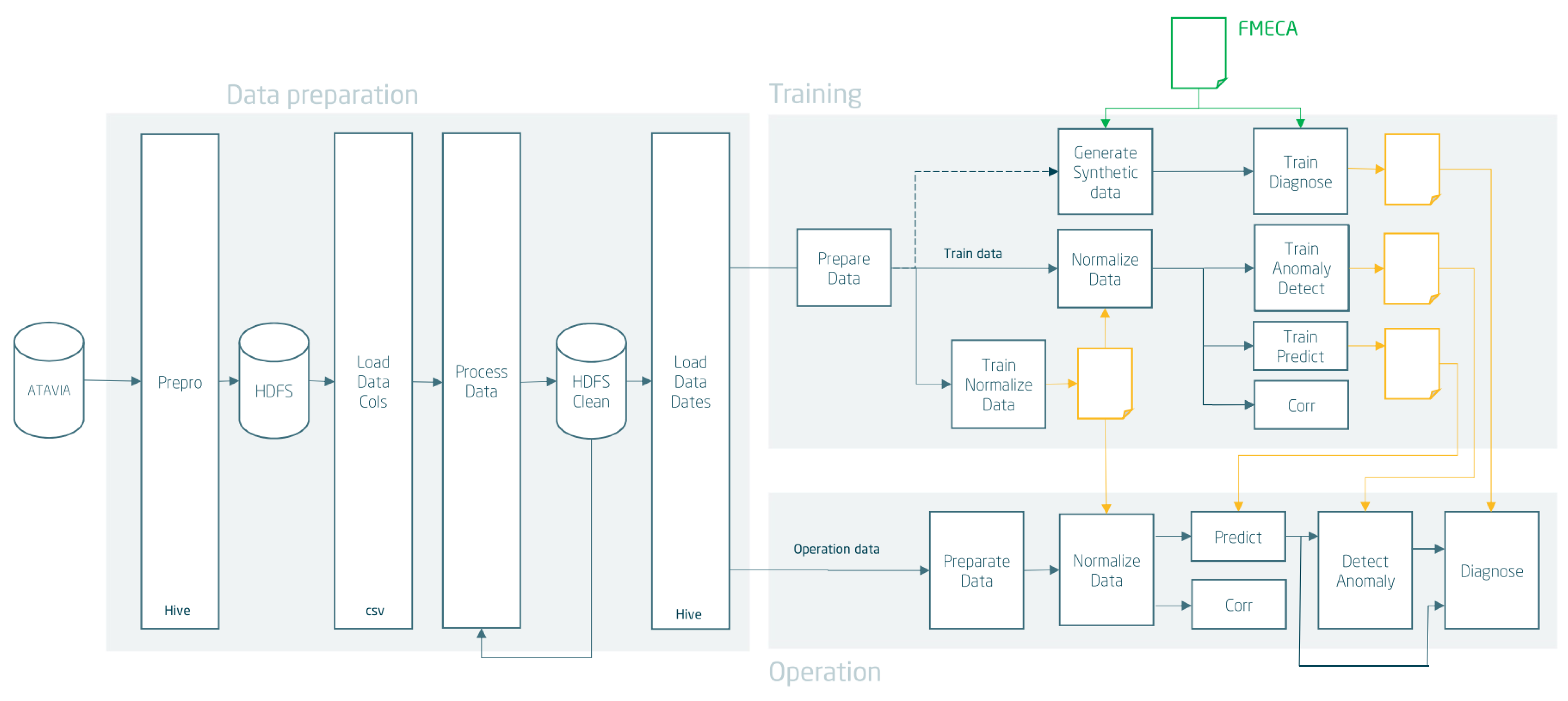
4. Unified Architecture

As defined in Section 2, a common approach was required in order to guarantee the scalability of the solution in terms of equipment and ship class. This approach had to deal with a variant number of features (from a few hundreds to thousands of inputs), acquisition frequencies (from mHz to Hz), algorithmic solutions and prediction horizons.
According to that, a modular architecture was designed where each one of the blocks could be modified (or even substituted) according to the necessities without altering the flow. As illustrated in Figure 1, this design differentiates three main parts: on the left side, the data processing modules are meant to be adequate for the input data to deal with it in the following steps. It includes the preprocessing (PrePro Data module) tasks required to structure the data into tabular information and the actual processing (Process Data). This second task involves cleaning, imputation, resampling and operational filtering. All of these subprocesses make use of the historical information previously cleaned and consolidated. The storage for both the raw data and the cleansed ones is performed in HDFS and recovered by using Hive queries. The combination of both make it possible to guarantee the robustness of the system and the availability of the information.
This information flows to the rest of the systemic parts (Training and Operation) through the subsequent Hive queries. These ones—depicted in the Filter Data module—retrieve and provide the required dataset (in terms of variables and time periods) for each one of the parts and blocks. The training and operation blocks are internally divided into three tasks, predicting the future state of the engine, detecting anomalies in that future state and diagnosing faults. The training block will train the models that carry out these tasks, while the operation block will apply these models to carry out predictive maintenance. In this sense, training modules require the longest historical possibilities for the equipment to be trained. This dataset is transformed, normalized and prepared (temporal aggregation and data split) so it can be ready for the prediction and anomaly detection algorithms (see Section 4.1 and Section 4.2, respectively). This grouping has been defined according to the operational requirements, which determines a triple scope s (days, weeks and months), providing then a triple time frame input to these modules. Finally, as stated in Section 2, there is a lack of supervised data required to postprocess the historical data: Synthetic data are generated using the dataset as the baseline and simulating malfunctions according to the FMECA parameters and conditions. As presented in Section 4.3, this modified dataset is the one used to train the diagnose algorithmic.
On the other hand, the operational block implements the predictive diagnosis. To this end, it repeats the data preparation and makes use of the training results—normalization, prediction, anomaly detection and diagnosing trained models—over the prepared incoming new data. In this sense, the system understands that any unconsolidated information segment is required to be processed. Thus, the operational modules are triggered either by batch processing (current data arrives periodically) or by the inclusion of relevant information from the past. In both cases, the resulting information is stored according to its time indexing.
Table 1 shows an example of FMECA entry as used in SOPRENE. It identifies the failure mode with a number that only serves as a label (31 in the example); for each failure mode, it provides a collection of variables along with their nominal values, threshold and tendency. This table contains implicit expert knowledge and identifies the signals that will be predicted, as explained in the next section.

4.1. Behavioural Prediction

The main objective is to estimate the state of a piece of equipment (such as the engine or the propeller) in a future instant of time. In this manner, in order to carry out a prediction from an instant of time t i s for a future instant that is distant from h o r i z o n units of time relative to the use of the engine ( t i + h o r i z o n s ), the system will use the information collected by the sensors during the previous w i n d o w units of time to t i s − ( t i w i n d o w s ). The user can customize the window size and prediction horizon, although by default, the horizon is used twice as the window size.
Both the h o r i z o n and the w i n d o w are relative to the time scope s selected (and, therefore, to the data aggregation performed). In this sense, despite the large data pools available during the preprocessing stage, the datasets resulting after the aggregation process are proportionally reduced. Thus, several predictions techniques have been considered for properly dealing with the precision requirements and the data load: on the one hand, regularized linear regression methods such as L1 (lasso) and L2 (ridge) have been used to deal with the slow degradative failures and the smaller dataset after the aggregation. Both techniques use the Spark MLlib library to provide distributed training and execution. On the other hand, Long Short-Term Memory (LSTM) based networks [36] have also been developed to make use of the massive data to forecast sudden and close-in-time events, although its the execution is not distributed.
The architecture keeps several aspects of predictive modeling open to maintain its flexibility. The final user is free to use the regression model, amount of training data, prediction and historic window length, among others, of his choice. This is performed in this manner because different equipment require different approaches. For example, using a LSTM network to model a collection of signals with data grouped by month and historic data along a couple of years will most likely overfit and, in that case, a lineal regression model will probably perform better.

4.2. Anomaly Detection

Once the prediction of the engine status has been made, it is necessary to determine whether this status corresponds to a normal value or a possible failure (anomaly). Since no labeled anomalies are available, the anomaly detection process is carried out in an unsupervised manner by using the autoencoder neural network. For the distributed implementation of this method, the Sparkling Water library was used.
By using the reconstruction error provided by the autoencoder model, we can discern between normal data (low reconstruction error) and anomalous data (high reconstruction error). This value can be presented as the mean square error of all the input variables (a single value) or its decomposition, that is, the error of each of the input variables or nodes of the network. The goal of this stage is to determine which ones are abnormal and which variables cause those abnormalities. The process is divided into three sequential phases:
  • Detect anomalies: To determine which datum is normal or anomalous, a first filter is carried out by using the mean square error. Based on a precalculated threshold error, the data that exceed this error are classified as anomalous and the rest as normal. The user can choose whether the calculation of this threshold error is carried out using the interquartile range technique [60] (a statistical dispersion measure that allows the threshold to be calculated automatically) or by establishing a percentage of anomalous data in the set of data.
  • Independent contributions: To determine which specific variables have caused the appearance of the anomaly in the data classified in the previous phase as anomalous, the decomposition of the reconstruction error is used (see Figure 2). Taking into account that the data are now normalized, this allows us to order the variables by their reconstruction error. To determine which variables have contributed the most to the formation of the anomaly, the system uses a method that automatically selects the most anomalous variables. The method is called the Elbow Method [61] and allows starting from a set of variables and their reconstruction errors by automatically selecting those that deviate the most.
  • Build anomaly mask: From the selection of the previous phase, a matrix or output mask of dimensions m × n is built and m is the number of rows or records and n is the number of columns or variables, where the anomalous variables are marked with a one and the normal variables with a zero. This information will be used by the subsequent diagnostic module.

4.3. Failure Diagnose

The diagnostic block is responsible for determining the failure mode by using the prediction data and the evaluation of the anomaly detection block when it occurs and the probability of each failure mode. In order to establish the probability, a set of Multilayer Perceptron [62] classifiers is used, which ranges from one to two hidden layers. In all the approaches, the number of neurons of the first hidden layer’s neurons triples the number of variables and decreases linearly until the output layer. In addition, RELU activation functions were used in all the hidden neurons, while sigmoid activations were used in the output layer to obtain the probabilities of the failures. Since labeled datasets corresponding to all possible failure modes are not available to train the perceptron, the decision was made with respect to implementing an artificial data generator in order to produce them. By studying the theoretical characteristics of the failure modes included in the FMECA document of the engine (variables involved, nominal values, range top values, etc.), the generator allows the creation of normal and anomalous datasets.
The system employs a perceptron to classify each failure mode. Each perceptron is trained with one failure mode asociated data; thus, when new data arrives, it issues the probability of occurrence of this failure mode. In this manner, each perceptron receives in its input layer the state of an engine (as many neurons as sensors) and emits in its output layer the probability of occurrence of the failure mode for which it has been trained (one neuron).
This classifier is used in combination with the mask generated by the anomalies detection block to perform the engine diagnostics. The utility of the failure mask is to narrow down the number of possible failure modes. Given a data record of an instant of time, for which the anomaly mask contains m variables marked as anomalous and n marked as normal, only the failure modes in which any of the m take part in will be considered as possible anomalous variables. In this manner, the failure modes in which all the variables involved have been considered normal by the anomaly detector will be omitted.

4.3.1. Artificial Failure Mode Generator

The FMECA document collects the nominal thresholds and range caps of the variables that make up each failure mode. By automatically analyzing this document, the system is able to obtain this information. The nominal value of a variable for a given failure mode is the usual value over which it oscillates without the failure mode occurring. The upper range values, however, are those minimum and maximum thresholds from which a sensor is in an abnormal state, which can result in the failure mode in question. The ranges of operating values of each variable, therefore, depend on the rest of the variables at each moment.
Since there are no labeled real data of each failure mode to train the models, based on the values described in the FMECA, the system is capable of generating artificial data associated with each failure mode. The variables that do not intervene in the failure mode will present values that oscillate above their corresponding nominal values, while the values of the variables that intervene in the failure mode will deviate beyond the upper range values associated with that failure mode. In order to avoid generating datasets that are too homogeneous, the system uses different kinds of distributions to introduce some variability in the sensors. For example, given an artificially generated dataset, the values taken by a variable that do not intervene in the generated failure mode will follow a normal distribution centered on the nominal value without reaching the upper range values.

4.3.2. Classification Model

The objective of the perceptrons is to determine if the status of a motor corresponds to any of the failure modes described in the FMECA document. Due to the use of a distributed version of the implementation, the system employs a model to classify each failure mode. In this manner, each perceptron receives in its input layer the state of a engine (as many neurons as sensors) and emits in its output layer the probability of occurrence of the failure mode for which it has been trained (one neuron). This output layer uses a softmax function to output a probability in the interval [0, 1].
The appearance of the system output is shown in Figure 3. Each row shows the identifier of the failure mode in the FMECA and the probability associated with each mode. For each column, the expected date on which the failure mode occurs is shown. The figure represents five failure modes labeled as 125, 44, 78, 18 and 82; the color represents the failure probability, with 0.5 marked as a white dot.

5. Results

The unified architecture has been implemented for two different scenarios, specifically for two types of engines: Diesel engines for propulsion of BAM Maritime Action Vessels and diesel engines for power generation in F-100 frigates. Although the architecture is common, the particularities of each scenario render some methods more appropriate than others and so there are low-level differences in implementation. In this section we describe the results obtained in the two case studies developed during the project.

5.1. Diesel Engine for Propulsion

The development has been subject to a mostly qualitative evaluation of the developers themselves and the organization involved. Some of these ideas are collected in this subsection:
  • Prediction: Despite the large data pools available, the RPM filtering rules out a significant piece of data when the engine was off. Due to this, when a large grouping is carried out (for example, 1 data/week or 1 data/month), very few data results. As stated in Section 4.1, it disables the correct convergence of certain models, making each one of them suitable for a specific scenario. Table 2 compares the different techniques and methods, collecting the mean squared errors by using different grouping modes and horizons.
    As it is possible to observe in the table, LSTM-based methods provide better performances with the lower degree of aggregation. Figure 4 depicts an example of prediction by using a recurrent neural network, where both sudden events and tendencies are correctly predicted. Please note that Figure 4 contains a prediction, while Figure 2 represents the reconstruction error in an autoencoder. On the other hand, Table 2 also illustrates that long-term behaviors are better estimated by simpler regression methods.
    The prediction system is very sensitive to both the grouping of the data and the sizes of the window and horizon. Furthermore, it has been found that, in general, there is a strong correlation between the variables that pass the selection process. A window size of approximately twice the forecast horizon has been found to be sufficient to achieve good results in most scenarios.
  • Anomaly detection: For this stage, two metrics have been used to qualitatively measure the performance of the model during an interval of four years: on the one hand, the anomalies detected by the model have been correlated with the warship’s engine alarm system. Although, this system does not collect malfunctions but operative conditions, it is possible to observe an indirect relation between them (see Figure 5). On the other hand, the results have been analyzed by maintenance experts which focused on specific known events. The unsupervised trained autoencoder model has been tested and the results have been satisfactory. The model was able to detect most of these anomalies, as can be observed in Figure 6. The value of this graph is found in the coincidences between signals along the x-axis.
    It should also be noted that this process is very sensitive to parameterization and can be configured to allow the passage of more or less anomalies through the reconstruction threshold and, within these, select a greater or lesser number of variables involved by using the Elbow Method parameters.
  • Failure diagnose: Using artificial datasets based on the engine’s design values (described in the Failure mode effects and criticality analysis, FMECA) has allowed us to build classification models that determine which failure modes are occurring. However, this theoretical behavior of the engine does not have to always correspond to reality, since its operation may vary with the use, replacement or repair of parts, etc. The training of diagnostic models depends directly on this generator and so it is necessary to build a sufficiently large and varied dataset.

5.2. Diesel Engine for Power Generation

The second case study involves the application of the SOPRENE architecture to the diesel engine for power generation in the F-100 class frigate. Each vessel contains four generators with six cylinders and the cylinders are in charge of generating the electrical power required by the ship. Despite the fact that engines for propulsion and power generation share a basic design, they pose interesting differences in order to validate the generality of the SOPRENE architecture.
For the purpose of this demonstrator, the main difference between propellant and power generation engines relies on the rotation velocity, which in the case of the power generator is, in essence, binary (stopped and online, with a brief transition state). Meanwhile, the propulsion engine has a continuous range of velocities, which requires more elaborate filtering techniques. A brief description of the main SOPRENE subsystems are as follows:
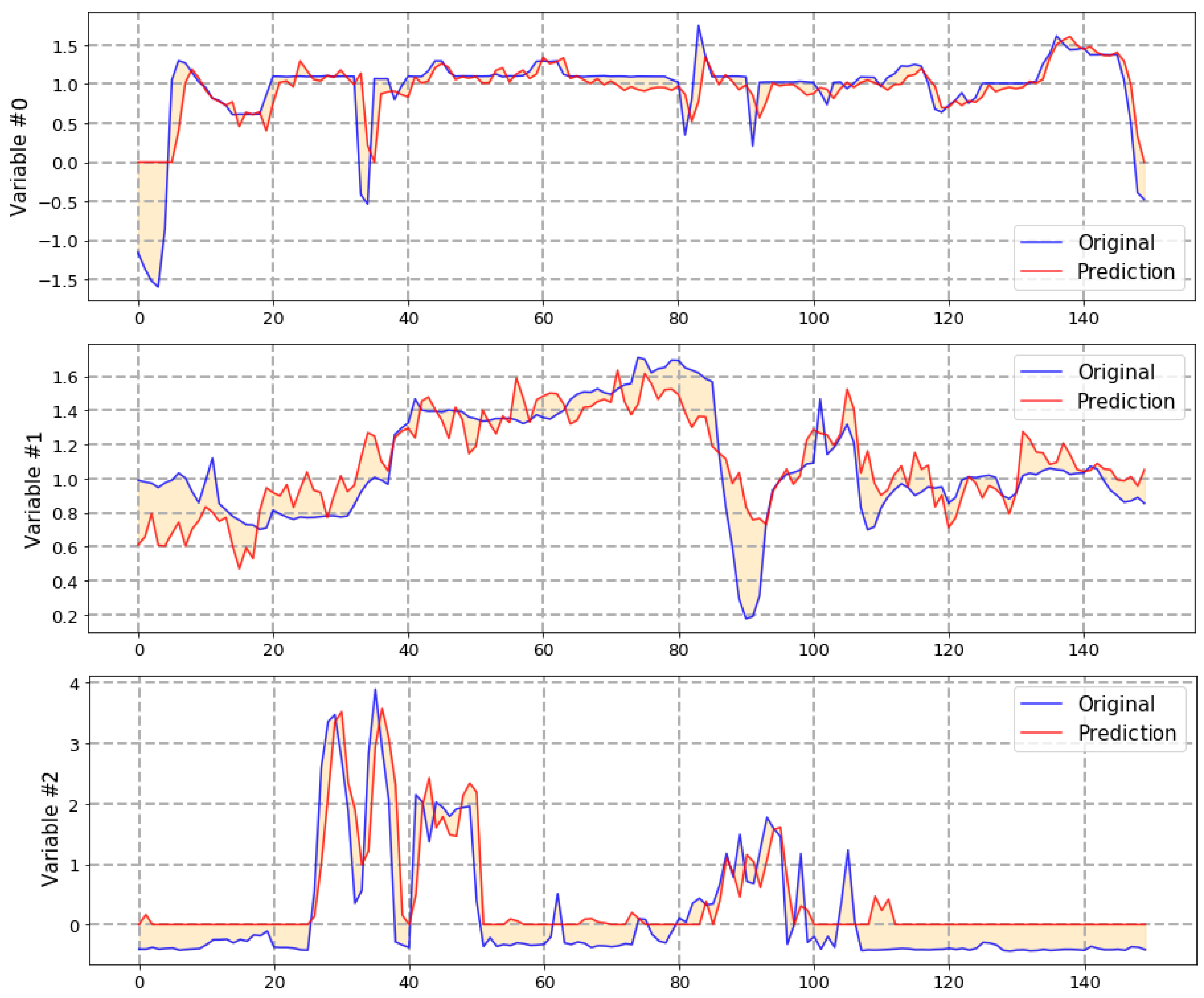
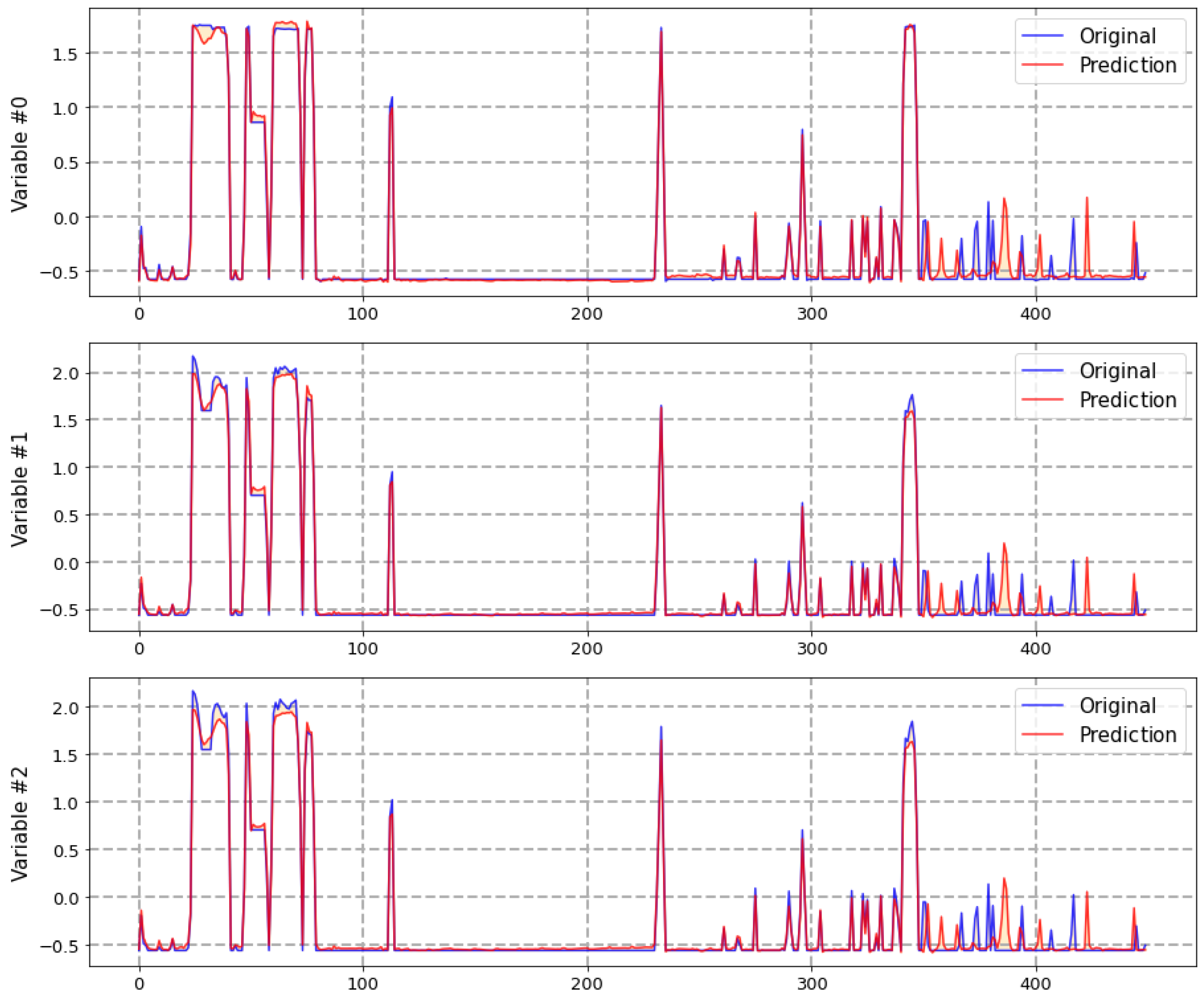
  • Prediction: Similarly to the propulsion engine, data grouping has a large impact on the amount of data available for training and validation of the diesel generator models. This happens even though the availability of a large amount of data (five ships with four engines each one) after aggregation and filtering the amount of available data for training and validation is limited. The flexibility of the SOPRENE architecture allowed the application of two types of models depending on the data aggregation: Deep LSTM networks for data grouped by days and weeks and regularized (L1, L2 and ElasticNet) lineal models for weeks and months. Linear models showed a strong tendency to underfit data grouped by days, while there were insufficient data to train LSTM networks with data grouped by months. Table 3 summarizes a comparison of the MSE measured in validation for lineal models and LSTM-based network for a 10 units prediction horizon; the best results are marked in bold. An example of prediction with a LSTM network can be observed in Figure 7 that shows three normalized variables corresponding to a certain FMECA failure mode.
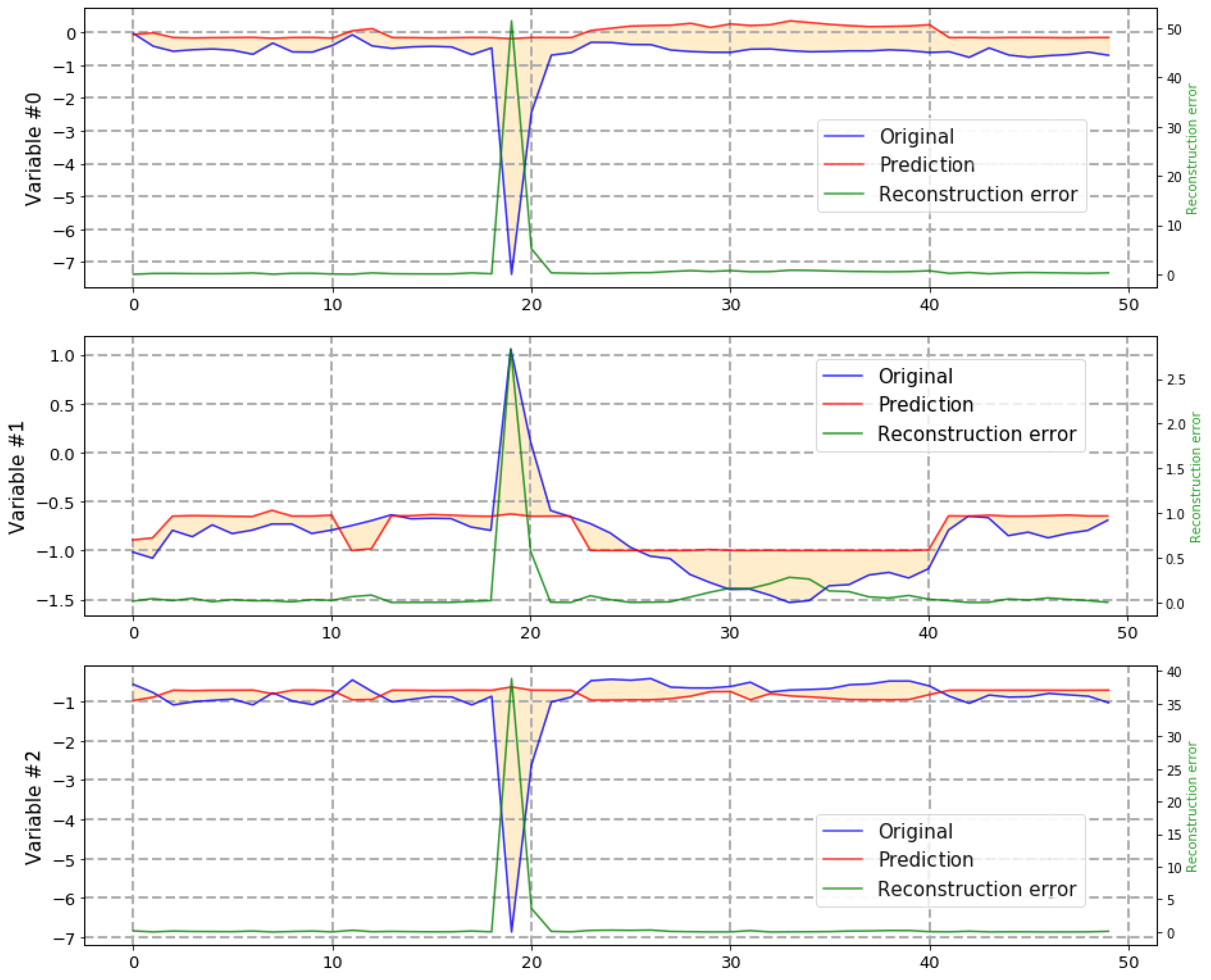
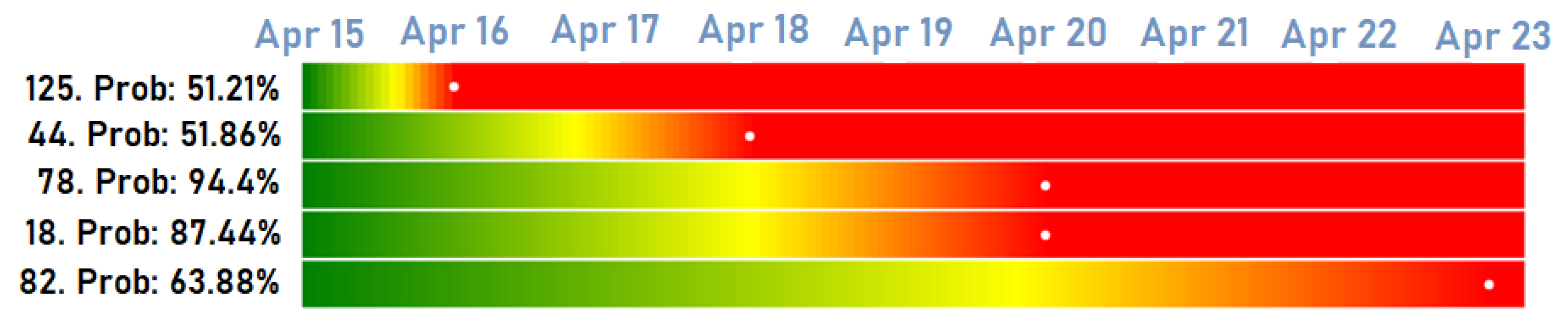
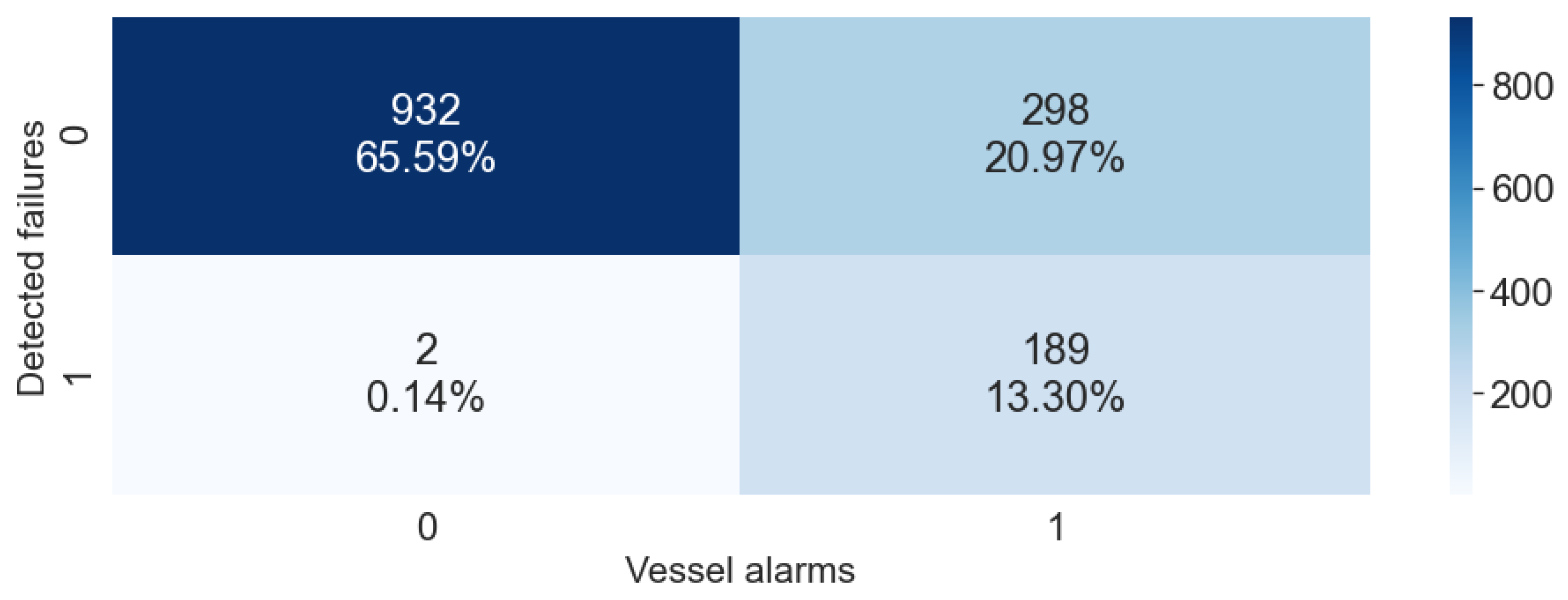
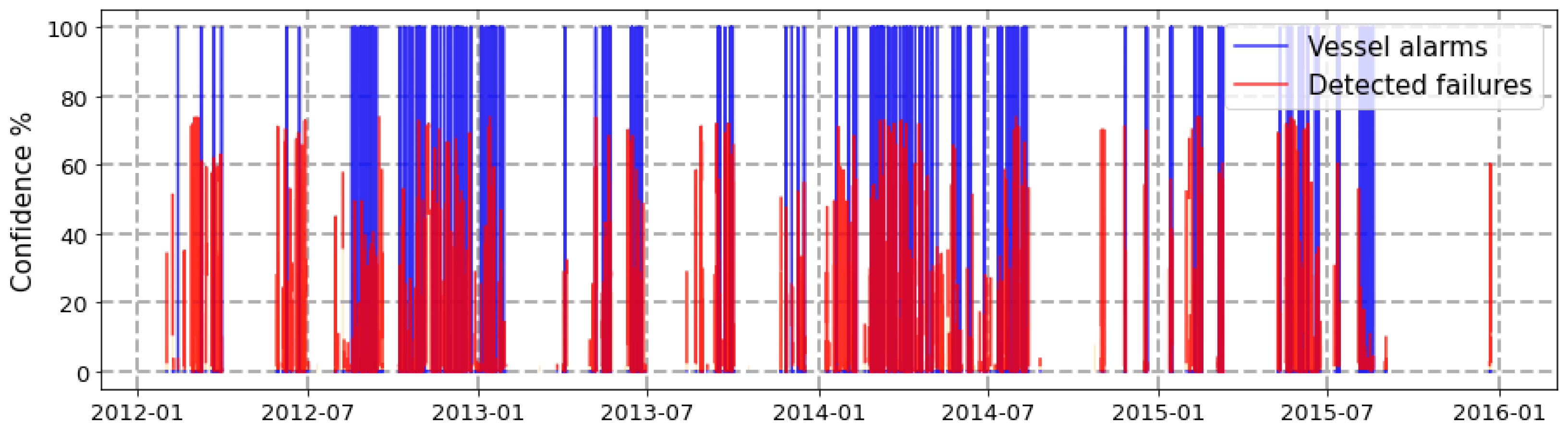
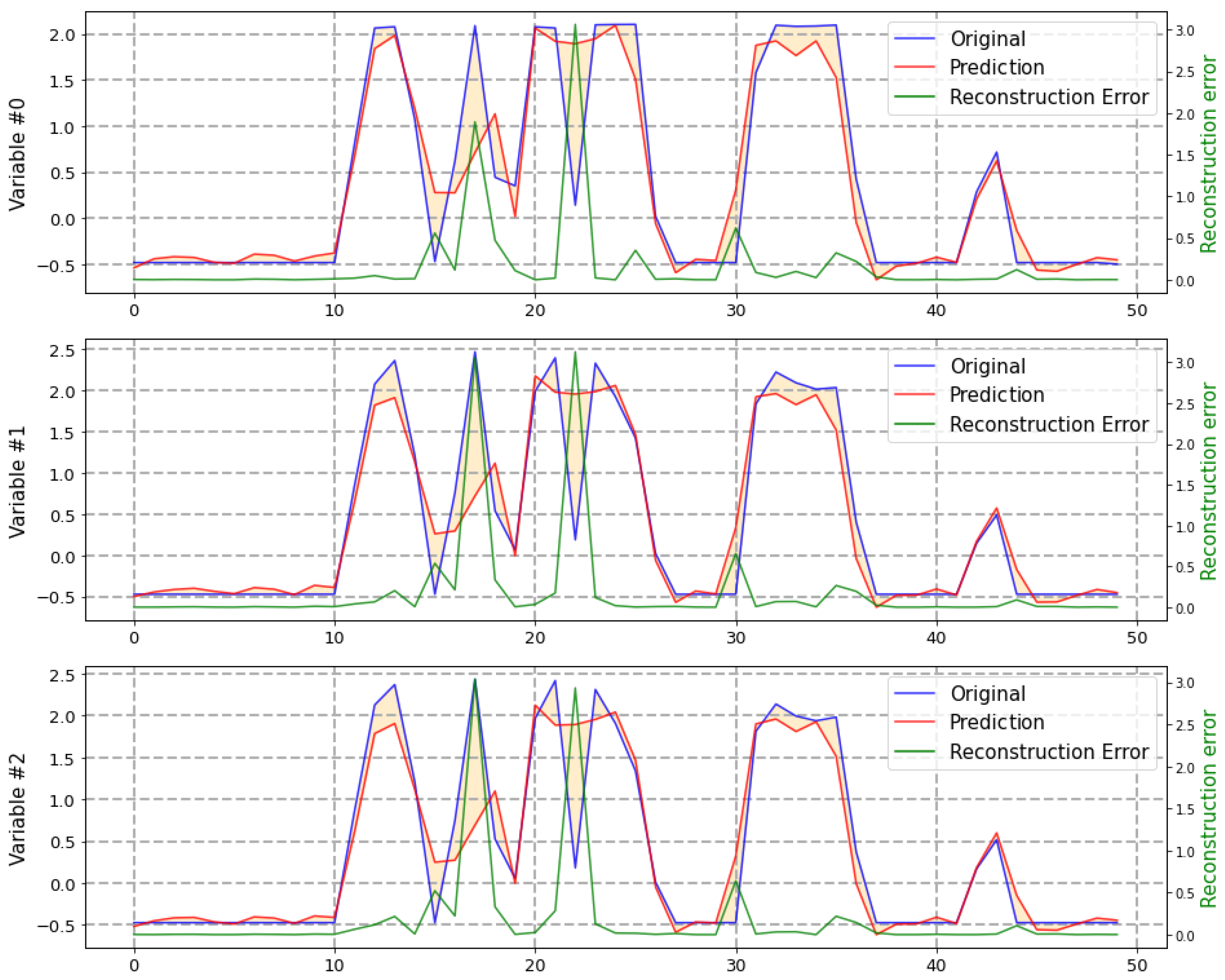
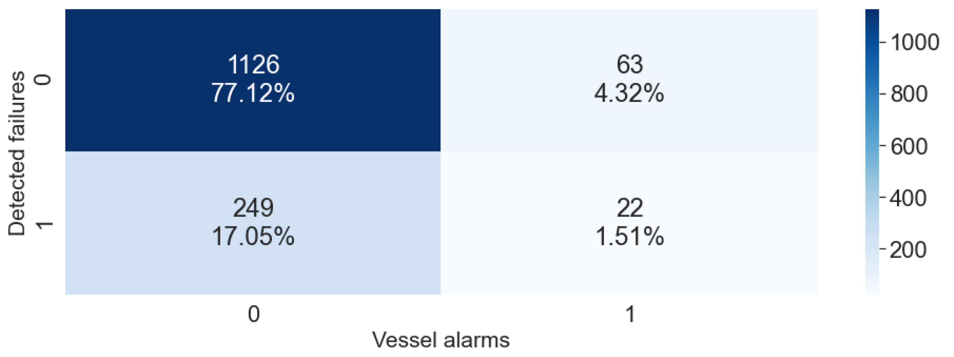
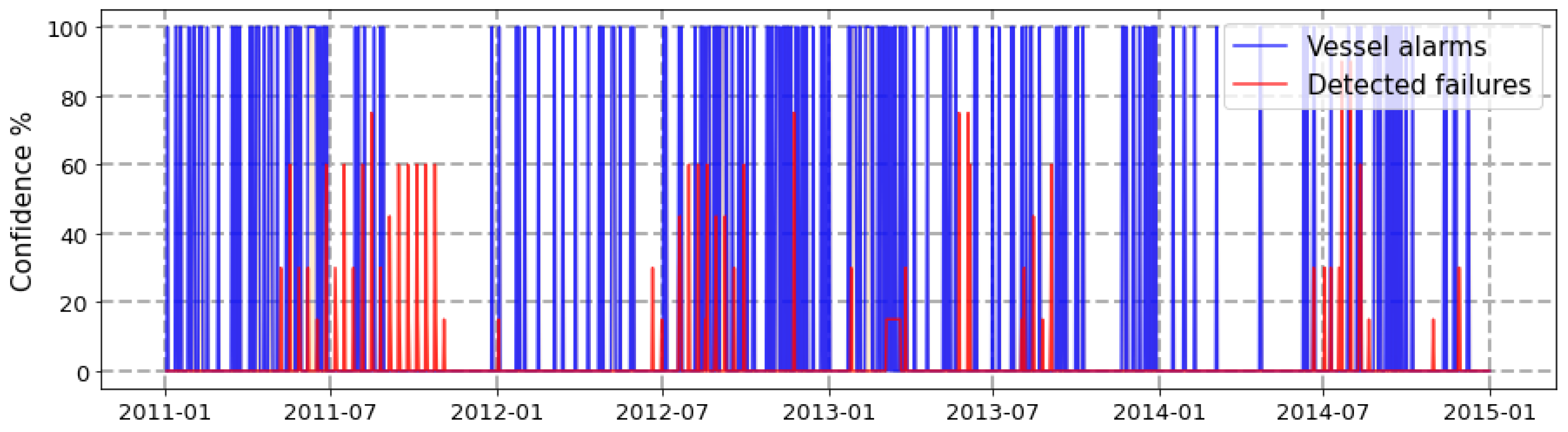
  • Anomaly detection: Given the lack of labeled data and the need to quantify the contribution of each attribute to the overall reconstruction error, we implemented the anomaly detection subsystem based on a deep LSTM autoencoder. The autoencoder input is composed by the signals identified by FMECA for a certain failure mode and the output is the reconstruction error of each one of this attributes. Figure 8 shows an example of the real values of three attributes compared with the output given by the autoconder. In this manner, the solution gains in interpretability while the overall reconstruction error is easily computed. Figure 9 shows a confusion matrix comparing the anomalies detected automatically with vessel alarms. Despite the unsupervised nature of the anomaly detector, it is able to detect anomalies that actually correspond to vessel alarms to a great extent. Figure 10 shows a different perspective of the anomaly detector. It shows a timeline with the vessels detected by human experts (blue) with the automatic anomaly detector (red). There is an evident difference in the level of confidence given by each detection method, but it is easily adjusted by a threshold.
  • Failure diagnosis: The main challenge in training the diagnosis model is to obtain a significant amount of data corresponding to the failure modes that are to be identified. Even though the datasets involved four years and five vessels, the presence of failure modes is limited in the extreme sense. A potential solution is to simulate the failure modes with thermodynamic models, but this was not an option in this context. The solution adopted was to synthesize data in each of the failure modes of interest by using the domain knowledge contained in FMECA. Of course the resulting synthetic dataset will not conserve all the complex behavior found in the engine, but the goal is actually to capture the information contained in FMECA with some variability to avoid overfitting. The system in charge of diagnosing the engine state for each failure mode identified in the FMECA is a MLP for which its input is the engine state and its output is a probability of occurrence of the given failure mode.

6. Conclusions

We have presented a scalable, robust and flexible predictive maintenance architecture for big and complex systems. It follows a modular design based on three independent blocks that can be modified, replaced or customized without altering the flow. It consists of the following: (1) a data processing module, (2) a data training module and (3) an operational module.
The virtues and limitations of this architecture have been verified and validated by the status monitoring of diverse diesel engine equipment (diesel engines for propulsion vessel’s propulsion and diesel generators) in two different ship classes of the Spanish Armada. In this sense, the data prediction, the detection of anomalies and the diagnosis of failure modes were carried out in two assets from a total of 28 tested in different vessels.
As shown along the paper, these predictions were correctly adjusted to what happened in different time horizons’ predictions. In the same manner, correct diagnoses of the probabilities of failure modes were carried out prior to the appearance of alarms on the monitored systems. In brief, the percentages of detectability were high enough to assume that this technological demonstrator is a great advancement in supporting human decisions of the human teams that are in charge of Spanish Armada’s units sustainment. Finally, the solution developed is a comprehensive system that allows the three predictive maintenance tasks (prognosis, anomaly detection and diagnosis) to be carried out in a reasonable time due to its distributed implementation, which allows working on large data sets (Big Data scenarios). In addition, it is valid for any ship in the fleet with similar characteristics and, due to its modularity, it can be easily adapted to new environments. To the best of our knowledge, this is the only complete predictive maintenance software for Big Data that has been used successfully in the naval sector. After this research study, we have verified that it is possible to define a general architecture that allows scalable predictive maintenance in a fleet of ships.
Several lines of work remain open. Given the flexibility of SOPRENE’s and the Spanish Armada’s needs, we plan to extend the platform to apply PdM to new equipment (fire extinguishers, naval electric engines, axes, etc.) and ships and, in this manner, reduce the maintenance cost of the fleet while increasing its operational capacity. One of the system limitations is that it has not been designed to operate in real-time and depends on complex offline processing in centralized data centers. To overcome this problem, we plan to extend SOPRENE by embedding it into the Spanish Armada’s ships operating in real-time with limited computational resources.

Author Contributions

Conceptualization, D.F.-B., O.F.-R. and D.S.; Data curation, D.N.-P.; Formal analysis, D.F.-B., O.F.-R., D.N.-P. and D.S.; Funding acquisition, F.L.-L.; Investigation, D.F.-B., O.F.-R. and D.N.-P.; Methodology, D.F.-B., O.F.-R. and D.S.; Project administration, F.L.-L. and D.S.; Resources, F.L.-L., D.F.-B. and O.F.-R.; Software, D.N.-P.; Supervision, D.S.; Validation, F.L.-L.; Writing—original draft, D.F.-B., O.F.-R., F.L.-L., D.N.-P., M.D.R.-M. and D.S. All authors have read and agreed to the published version of the manuscript.

Funding

This research was funded by DGAM-PLATIN (General Directorate of Armament and Material—Spanish Ministry of Defence) with project funding number ‘2018/1003218001400’.

Data Availability Statement

Data sharing not applicable (Confidential data).

Acknowledgments

This paper reports part of the results obtained within the ‘SOPRENE’ research and development project funded by DGAM-PLATIN (General Directorate of Armament and Material—Spanish Ministry of Defence). This project developed a technological demonstrator of AI techniques and applications over naval platform assets for predictive maintenance purposes. The authors are also grateful to all the Spanish Armada’s units that have participated in some manner in the obtaining of these results and for providing their technical advice in FMECA development, without which this assessment of AI techniques would not be accomplished.

Conflicts of Interest

The authors declare no conflict of interest.

References

  1. Mobley, K. An Introduction to Predictive Maintenance; Elsevier: Amsterdam, The Netherlands, 2002. [Google Scholar]
  2. Huda, A.N.; Taib, S. Application of infrared thermography for predictive/preventive maintenance of thermal defect in electrical equipment. Appl. Therm. Eng. 2013, 61, 220–227. [Google Scholar] [CrossRef]
  3. Durocher, D.B.; Feldmeier, G.R. Predictive versus preventive maintenance. IEEE Ind. Appl. Mag. 2004, 10, 12–21. [Google Scholar] [CrossRef]
  4. Selcuk, S. Predictive maintenance, its implementation and latest trends. Proc. Inst. Mech. Eng. Part B J. Eng. Manuf. 2017, 231, 1670–1679. [Google Scholar] [CrossRef]
  5. Motaghare, O.; Pillai, A.S.; Ramachandran, K.I. Predictive Maintenance Architecture. In Proceedings of the 2018 IEEE International Conference on Computational Intelligence and Computing Research (ICCIC), Madurai, India, 13–15 December 2018; pp. 1–4. [Google Scholar] [CrossRef]
  6. Kanawaday, A.; Sane, A. Machine learning for predictive maintenance of industrial machines using IoT sensor data. In Proceedings of the 2017 8th IEEE International Conference on Software Engineering and Service Science (ICSESS), Beijing, China, 24–26 November 2017; pp. 87–90. [Google Scholar]
  7. Canizo, M.; Onieva, E.; Conde, A.; Charramendieta, S.; Trujillo, S. Real-time predictive maintenance for wind turbines using Big Data frameworks. In Proceedings of the 2017 IEEE International Conference on Prognostics and Health Management (ICPHM), Dallas, TX, USA, 19–21 June 2017; pp. 70–77. [Google Scholar]
  8. Wang, J.; Liang, Y.; Zheng, Y.; Gao, R.X.; Zhang, F. An integrated fault diagnosis and prognosis approach for predictive maintenance of wind turbine bearing with limited samples. Renew. Energy 2020, 145, 642–650. [Google Scholar] [CrossRef]
  9. Budai, G.; Huisman, D.; Dekker, R. Scheduling preventive railway maintenance activities. J. Oper. Res. Soc. 2006, 57, 1035–1044. [Google Scholar] [CrossRef] [Green Version]
  10. Byington, C.S.; Roemer, M.J.; Galie, T. Prognostic enhancements to diagnostic systems for improved condition-based maintenance [military aircraft]. In Proceedings of the IEEE Aerospace Conference, Big Sky, MT, USA, 9–16 March 2002; Volume 6, p. 6. [Google Scholar]
  11. Fernández Jove, A.; Mackinlay, A.; Riola, J.M. Optimization of the Life Cycle in the Warships: Maintenance Plan and Monitoring for Costs Reduction. In Proceedings of the VI International Ship Design & Naval Engineering Congress (CIDIN) and XXVI Pan-American Congress of Naval Engineering, Maritime Transportation and Port Engineering (COPINAVAL); Springer: Cham, Switzerland, 2019; pp. 391–401. [Google Scholar]
  12. Lamas-López, F. Evolution of logistical support in the Spanish Navy through 4.0 technologies. In Proceedings of the 18th Conference of the Spanish Association for Artificial Intelligence (CAEPIA), Granada, Spain, 23–26 October 2018; pp. 1345–1350. [Google Scholar]
  13. IEC. Failure Modes and Effects Analysis (FMEA and FMECA); Technical Report, IEC Standard Number 60812:2018; International Electrotechnical Commission: London, UK, 2018. [Google Scholar]
  14. Ran, Y.; Zhou, X.; Lin, P.; Wen, Y.; Deng, R. A Survey of Predictive Maintenance: Systems, Purposes and Approaches. arXiv 2019, arXiv:1912.07383. [Google Scholar]
  15. He, Y.; Han, X.; Gu, C.; Chen, Z. Cost-oriented predictive maintenance based on mission reliability state for cyber manufacturing systems. Adv. Mech. Eng. 2018, 10, 1687814017751467. [Google Scholar] [CrossRef] [Green Version]
  16. Lin, L.; Luo, B.; Zhong, S. Multi-objective decision-making model based on CBM for an aircraft fleet with reliability constraint. Int. J. Prod. Res. 2018, 56, 4831–4848. [Google Scholar] [CrossRef]
  17. Zhao, J.; Yang, L. A bi-objective model for vessel emergency maintenance under a condition-based maintenance strategy. Simulation 2018, 94, 609–624. [Google Scholar] [CrossRef]
  18. Xiang, Y.; Coit, D.; Zhu, Z. A Multi-objective Joint Burn-in and Imperfect Condition-based Maintenance Model for Degradation-based Heterogeneous Populations. Qual. Reliab. Eng. Int. 2016, 32, 2739–2750. [Google Scholar] [CrossRef]
  19. Song, S.; Coit, D.W.; Feng, Q. Reliability analysis of multiple-component series systems subject to hard and soft failures with dependent shock effects. IIE Trans. 2016, 48, 720–735. [Google Scholar] [CrossRef]
  20. Gravette, M.A.; Barker, K. Achieved availability importance measure for enhancing reliability-centered maintenance decisions. Proc. Inst. Mech. Eng. Part O J. Risk Reliab. 2015, 229, 62–72. [Google Scholar] [CrossRef]
  21. Konys, A. An Ontology-Based Knowledge Modelling for a Sustainability Assessment Domain. Sustainability 2018, 10, 300. [Google Scholar] [CrossRef] [Green Version]
  22. Peng, Y.; Dong, M.; Zuo, M.J. Current status of machine prognostics in condition-based maintenance: A review. Int. J. Adv. Manuf. Technol. 2010, 50, 297–313. [Google Scholar] [CrossRef]
  23. Chen, N.; Ye, Z.S.; Xiang, Y.; Zhang, L. Condition-based mainte-nance using the inverse gaussian degradation model Assessment Domain. Eur. J. Oper. Res. 2015, 243, 190–199. [Google Scholar] [CrossRef]
  24. Lucifredi, A.; Mazzieri, C.; Rossi, M. Application of multiregressive linear models, dynamic kriging models and neural network models to predictive maintenance of hydroelectric power systems. Mech. Syst. Signal Process. 2000, 14, 471–494. [Google Scholar] [CrossRef]
  25. Calder, M.; Sevegnani, M. Stochastic Model Checking for Predicting Component Failures and Service Availability. IEEE Trans. Dependable Secur. Comput. 2019, 16, 174–187. [Google Scholar] [CrossRef] [Green Version]
  26. Samanta, B.; Al-Balushi, K. Artificial Neural Network based fault diagnostics of rolling element bearings using time-domain features. Mech. Syst. Signal Process. 2003, 17, 317–328. [Google Scholar] [CrossRef]
  27. Quinlan, J.R. Improved Use of Continuous Attributes in C4.5. J. Artif. Intell. Res. 1996, 4, 77–90. [Google Scholar] [CrossRef] [Green Version]
  28. Shi, J.; Niu, N.; Zhu, X. A Fault Diagnosis Method for Multi-Condition System Based on Random Forest. In Proceedings of the 2019 Prognostics and System Health Management Conference (PHM-Paris), Paris, France, 2–5 May 2019; pp. 350–355. [Google Scholar]
  29. Chen, Y.; He, Y.; Li, Z.; Chen, L.; Zhang, C. Remaining Useful Life Prediction and State of Health Diagnosis of Lithium-ion Battery based on Second-order Central Difference Particle Filter. IEEE Access 2020, 8, 37305–37313. [Google Scholar] [CrossRef]
  30. Ratsch, G.; Mika, S.; Scholkopf, B.; Muller, K. Constructing boosting algorithms from SVMs: An application to one-class classification. IEEE Trans. Pattern Anal. Mach. Intell. 2002, 24, 1184–1199. [Google Scholar] [CrossRef] [Green Version]
  31. Susto, G.A.; Schirru, A.; Pampuri, S.; McLoone, S.; Beghi, A. Machine Learning for Predictive Maintenance: A Multiple Classifier Approach. IEEE Trans. Ind. Inform. 2015, 11, 812–820. [Google Scholar] [CrossRef] [Green Version]
  32. Liu, Z.; Mei, W.; Zeng, X.; Yang, C.; Zhou, X. Remaining Useful Life Estimation of Insulated Gate Biploar Transistors (IGBTs) Based on a Novel Volterra k-Nearest Neighbor Optimally Pruned Extreme Learning Machine (VKOPP) Model Using Degradation Data. Sensors 2017, 17, 2524. [Google Scholar] [CrossRef] [PubMed] [Green Version]
  33. Chen, X.L.; Wang, P.H.; Hao, Y.S.; Zhao, M. Evidential KNN-based condition monitoring and early warning method with applications in power plant. Neurocomputing 2018, 315, 18–32. [Google Scholar] [CrossRef]
  34. Ma, M.; Sun, C.; Chen, X. Deep Coupling Autoencoder for Fault Diagnosis With Multimodal Sensory Data. IEEE Trans. Ind. Inform. 2018, 14, 1137–1145. [Google Scholar] [CrossRef]
  35. Yuan, J.; Tian, Y. An Intelligent Fault Diagnosis Method Using GRU Neural Network towards Sequential Data in Dynamic Processes. Processes 2019, 7, 152. [Google Scholar] [CrossRef] [Green Version]
  36. Yang, R.; Huang, M.; Lu, Q.; Zhong, M. Rotating Machinery Fault Diagnosis Using Long-short-term Memory Recurrent Neural Network. IFAC PapersOnLine 2018, 51, 228–232. [Google Scholar] [CrossRef]
  37. Simões, A.; Viegas, J.M.; Farinha, J.T.; Fonseca, I. The State of the Art of Hidden Markov Models for Predictive Maintenance of Diesel Engines. Qual. Reliab. Eng. Int. 2017, 33, 2765–2779. [Google Scholar] [CrossRef]
  38. Nixon, S.; Weichel, R.; Reichard, K.; Kozlowski, J. A machine learning approach to diesel engine health prognostics using engine controller data. In Proceedings of the PHM2018—Annual Conference of the Prognostics and Health Management Society, Philadelphia, PA, USA, 24–27 September 2018. [Google Scholar]
  39. Hong, C.W.; Lee, C.; Lee, K.; Ko, M.S.; Kim, D.E.; Hur, K. Remaining useful life prognosis for turbofan engine using explainable deep neural networks with dimensionality reduction. Sensors 2020, 20, 6626. [Google Scholar] [CrossRef]
  40. UNCTAD. Review of Maritime Transport; Technical Report UNCTAD/RMT/2015; United Nations Conference on Trade and Development: New York, NY, USA, 2015. [Google Scholar]
  41. Karatuğ, Ç.; Arslanoğlu, Y. Importance of early fault diagnosis for marine diesel engines: A case study on efficiency management and environment. Ships Offshore Struct. 2020. [Google Scholar] [CrossRef]
  42. Lazakis, I.; Gkerekos, C.; Theotokatos, G. Investigating an SVM-driven, one-class approach to estimating ship systems condition. Ships Offshore Struct. 2019, 14, 432–441. [Google Scholar] [CrossRef]
  43. Stopford, M. Maritime Economics 3e; Routledge: London, UK, 2008. [Google Scholar]
  44. Park, P.; Marco, P.D.; Shin, H.; Bang, J. Fault detection and diagnosis using combined autoencoder and long short-term memory network. Sensors 2019, 19, 4612. [Google Scholar] [CrossRef] [PubMed] [Green Version]
  45. Tsitsilonis, K.M.; Theotokatos, G. Engine malfunctioning conditions identification through instantaneous crankshaft torque measurement analysis. Appl. Sci. 2021, 11, 3522. [Google Scholar] [CrossRef]
  46. Bampoula, X.; Siaterlis, G.; Nikolakis, N.; Alexopoulos, K. A Deep Learning Model for Predictive Maintenance in Cyber-Physical Production Systems Using LSTM Autoencoders. Sensors 2021, 21, 972. [Google Scholar] [CrossRef] [PubMed]
  47. Kim, D.G.; Choi, J.Y. Optimization of Design Parameters in LSTM Model for Predictive Maintenance. Appl. Sci. 2021, 11, 6450. [Google Scholar] [CrossRef]
  48. Wu, J.Y.; Wu, M.; Chen, Z.; Li, X.L.; Yan, R. Degradation-Aware Remaining Useful Life Prediction With LSTM Autoencoder. IEEE Trans. Instrum. Meas. 2021, 70, 1–10. [Google Scholar] [CrossRef]
  49. Liu, Q.; Liu, S.; Dai, Q.; Yu, X.; Teng, D.; Wei, M. Data-Driven Approaches for Diagnosis of Incipient Faults in Cutting Arms of the Roadheader. Shock Vib. 2021, 2021, 8865068. [Google Scholar] [CrossRef]
  50. Li, T.; Hua, M.; Yin, Q. The Temperature Forecast of Ship Propulsion Devices from Sensor Data. Information 2019, 10, 316. [Google Scholar] [CrossRef] [Green Version]
  51. Coraddu, A.; Oneto, L.; Ghio, A.; Savio, S.; Anguita, D.; Figari, M. Machine learning approaches for improving condition-based maintenance of naval propulsion plants. Proc. Inst. Mech. Eng. Part M J. Eng. Marit. Environ. 2016, 230, 136–153. [Google Scholar] [CrossRef]
  52. Cai, B.; Sun, X.; Wang, J.; Yang, C.; Wang, Z.; Kong, X.; Liu, Z.; Liu, Y. Fault detection and diagnostic method of diesel engine by combining rule-based algorithm and BNs/BPNNs. J. Manuf. Syst. 2020, 57, 148–157. [Google Scholar] [CrossRef]
  53. Gkerekos, C.; Lazakis, I.; Theotokatos, G. Machine learning models for predicting ship main engine Fuel Oil Consumption: A comparative study. Ocean Eng. 2019, 188, 106282. [Google Scholar] [CrossRef]
  54. Uyanık, T.; Karatuğ, Ç.; Arslanoğlu, Y. Machine learning approach to ship fuel consumption: A case of container vessel. Transp. Res. Part D Transp. Environ. 2020, 84, 102389. [Google Scholar] [CrossRef]
  55. Cheliotis, M.; Gkerekos, C.; Lazakis, I.; Theotokatos, G. A novel data condition and performance hybrid imputation method for energy efficient operations of marine systems. Ocean Eng. 2019, 188, 106220. [Google Scholar] [CrossRef]
  56. Tan, Y.; Niu, C.; Tian, H.; Lin, Y.; Zhang, J. Decay detection of a marine gas turbine with contaminated data based on isolation forest approach. Ships Offshore Struct. 2021, 16, 546–556. [Google Scholar] [CrossRef]
  57. Makridis, G.; Kyriazis, D.; Plitsos, S. Predictive maintenance leveraging machine learning for time-series forecasting in the maritime industry. In Proceedings of the 2020 IEEE 23rd International Conference on Intelligent Transportation Systems (ITSC), Rhodes, Greece, 20–23 September 2020; pp. 1–8. [Google Scholar] [CrossRef]
  58. Tan, Y.; Niu, C.; Tian, H.; Hou, L.; Zhang, J. A one-class SVM based approach for condition-based maintenance of a naval propulsion plant with limited labeled data. Ocean Eng. 2019, 193, 106592. [Google Scholar] [CrossRef]
  59. Smart, E.; Grice, N.; Ma, H.; Garrity, D.; Brown, D. One class classification based anomaly detection for marine engines. In Intelligent Systems: Theory, Research and Innovation in Applications; Studies in Computational Intelligence; Springer International Publishing: Cham, Switzerland, 2020; Volume 864, pp. 223–245. [Google Scholar] [CrossRef]
  60. Frey, B.B. (Ed.) The SAGE Encyclopedia of Educational Research, Measurement, and Evaluation; AGE Publications, Inc.: Thousand Oaks, CA, USA, 2018. [Google Scholar]
  61. Bholowalia, P.; Kumar, A. Article: EBK-Means: A Clustering Technique based on Elbow Method and K-Means in WSN. Int. J. Comput. Appl. 2014, 105, 17–24. [Google Scholar]
  62. Marius, P.; Balas, V.; Perescu-Popescu, L.; Mastorakis, N. Multilayer perceptron and neural networks. WSEAS Trans. Circuits Syst. 2009, 8, 579–588. [Google Scholar]
Figure 1. Architectural design. SOPRENE is composed by three big subsystems: processing, training and operation. Processing subsystem is common to training and operation.
Applsci 11 07322 g001
Figure 2. Autoencoder output (red) versus the original value to be reconstructed (blue) and the associated reconstruction error (green) for three attributes of the diesel engine for propulsion. x-axis represents normalized data coming from a BAM-class (Maritime Action Vessels) ship; y-axis contains an ordered index. Reconstruction error rises when the autoencoder is unable to reproduce the signals.
Applsci 11 07322 g002
Figure 3. Example of system output for five failure modes (named 125, 44, 78, 18 and 82) sorted temporally. Each row depicts the evolution of the probability of failure along the time. The points where the failure probability reaches its peak are marked with white dots.
Applsci 11 07322 g003
Figure 4. Long-Short Term Memory Networks (LSTM) prediction output (red) versus the real value to be predicted (blue) for three attributes of the diesel engine for propulsion. X-axis represents normalized data coming from the BAM ship; y-axis contains an ordered index. Shadowed area represents prediction error.
Applsci 11 07322 g004
Figure 5. Confusion matrix of the failures detected by the BAM’s engine alarm system versus the anomalies detected by the model.
Applsci 11 07322 g005
Figure 6. Normalized comparison of the vessel alarms (in blue) with the autoencoder’s joint diagnostics for all failure modes. Data comes from a BAM ship. y-axis represents the confidence given by the autoencoder. x-axis represents normalized data coming from the vessel.
Applsci 11 07322 g006
Figure 7. LSTM forecasting output (red) versus the real value (blue) for three variables of the diesel generator. Y-axis depicts the value of the variable. X-axis represents normalized data coming from the vessel.
Applsci 11 07322 g007
Figure 8. LSTM autoencoder output (red) with the contribution of each attribute (green) and the original value (blue) for the diesel generator.
Applsci 11 07322 g008
Figure 9. Confusion matrix comparing detected failures vs. vessel alarms for the power-generation engine in the F-100 class frigate.
Applsci 11 07322 g009
Figure 10. Normalized comparison of the vessel alarms (in blue) with the autoencoder’s joint diagnostics for all failure modes. Data comes from a F-100 class frigate. Y-axis represents the confidence given by the autoencoder. X-axis represents normalized data coming from the vessel.
Applsci 11 07322 g010
Table 1. Example of failure mode identified by the failure mode, effects and criticality analysis (FMECA). This failure mode has an Id 31 and comprises three signals. Values shown do not correspond to any real failure mode.
IdSignalNominal ValueThreshold ValueTendency
31Variable 11.32
Variable 25.45
Variable 35560
Table 2. Mean squared errors (MSE) obtained by the algorithms using different data grouping modes: 1 data/day (D), 1 data/week (W) and 1 data/month (M). The prediction horizons used were 5 and 10 units.
Horizon = 5Horizon = 10
AlgorithmDWMHDW
Linear Regression0.650.360.220.640.350.27
L10.620.360.220.610.320.25
L20.600.330.200.640.310.24
Elastic Net0.560.320.150.570.330.06
LSTM0.410.280.160.400.270.16
Table 3. Mean squared errors (MSE) obtained by the algorithms by using different data grouping modes for power-generation engine: 1 data/day (D), 1 data/week (W) and 1 data/month. The prediction horizons used were 10 units.
AlgorithmDWM
Linear Regression- 1.65 1.66
L1- 0.79 0.49
L2- 3.0 0.53
Elastic Net- 0.79 0.525
LSTM0.310.59-
Publisher’s Note: MDPI stays neutral with regard to jurisdictional claims in published maps and institutional affiliations.

