Article

How to Quantify the Dynamics of Single (Straight or Sinuous) and Multiple (Anabranching) Channels from Imagery for River Restoration

1
UFR Geography, History, Economy and Societies, UMR 8586 PRODIG, University of Paris, Case 7001, 5 Rue Thomas Mann, CEDEX 13, F-75205 Paris, France
2
Research and Scientific Support Department, French National Agency for Biodiversity, 5 Square Félix Nadar, F-94300 Vincennes, France
3
LHSV—Saint-Venant Hydraulics Laboratory, 6 Quai Watier, F-78400 Chatou, France
*
Author to whom correspondence should be addressed.
Appl. Sci. 2021, 11(17), 8075; https://doi.org/10.3390/app11178075
Submission received: 1 July 2021 / Revised: 9 August 2021 / Accepted: 26 August 2021 / Published: 31 August 2021

Abstract

:
Since the 2000s, European rivers have undergone restoration works to give them back a little more ‘freedom space’ and consolidate the hydro-sedimentary continuum and biological continuity as required by the Water Framework Directive (WFD). In high-energy rivers, suppression of lateral constraints (embankment removal) leads to geomorphological readjustments in the modification of both the active-channel length and active-channel width. The article provides a new methodological development to overcome the shortcomings of traditional methods (based on diachronic cross-section analysis) unable to simultaneously take into account these geometric adjustments after active-channel restoration. It allows us to follow and precisely quantify the geomorphological changes of the active channel faced to the stakes (i.e., structures or urbanized, recreation or agricultural areas) in the floodplain. The methodology proposes three new indicators (distance from active channel to stakes or floodplain margins as indicator 1; distance from stakes to active channel as indicator 2; diachronic distance as indicator 3) and a metric analysis grid in the 2D Euclidean space. It is applied to the Clamoux River (order 4, Strahler; bankfull, specific stream power: 280 W/m2) in the Aude watershed (Mediterranean France). The paper shows the full potential of this methodological protocol to be able to meet managers’ expectations as closely as possible within the framework of the multi-annual active-channel monitoring.

1. Introduction

Today, many rivers around the world no longer exhibit their natural, morphological features because they have undergone significant modifications at least since the eighteenth–nineteenth century, through hydroclimate change and anthropogenic actions, as the channelization, construction of dikes, weirs and dams, river embankments and meanders cutting (Figure 1). Focusing on the human impact, hydraulic structures, whether longitudinal or transverse to the flow, have affected the proper hydromorphological and sediment functioning of rivers, thereby impacting biological conditions and significantly reducing biodiversity along the alluvial corridors. The scientific community and the managers of hydrosystems are now raising the question of how to give rivers balanced hydrological, morphological and sedimentary functioning, thus notably helping them to achieve the good ecological status of waterbodies by increasing water quality, morphological diversity and resilience to climate change and/or anthropogenic alterations. This paradigm corresponds to what is often called ‘river restoration’.
In this paper, we focused on one type of river restoration, which concerns actions that can help to give more lateral space to rivers (Figure 2) by removing longitudinal structures (gabions, walls, dikes, embankments or other riverbank protections) along the channels (for an exhaustive and complete review on river restoration, see [29,30,31]). Allowing rivers to obtain more lateral migration capacity amounts to working on the ‘river space of good functioning’ [32], i.e., the space that the river needs to regulate erosion processes at the watershed scale as well as low-waters and floods thanks to the reactivation of the margins of the active channel. Most of the time, river channelization has resulted in the simplification and shortening of streams, reduction of channel sinuosity and increase in the hydraulic slope and bed shear stress. This was the case for the braided rivers, which were channelized (Figure 2, Stage 2A). Sometimes, the channel pattern of the rivers has been modified from braided to meandering channel (Figure 2, Stage 2B), which has led to lengthening the watercourse and reducing the energy slope and specific stream power.
From this operating model, we can distinguish three stages in the recent history of rivers (Table 1):
-
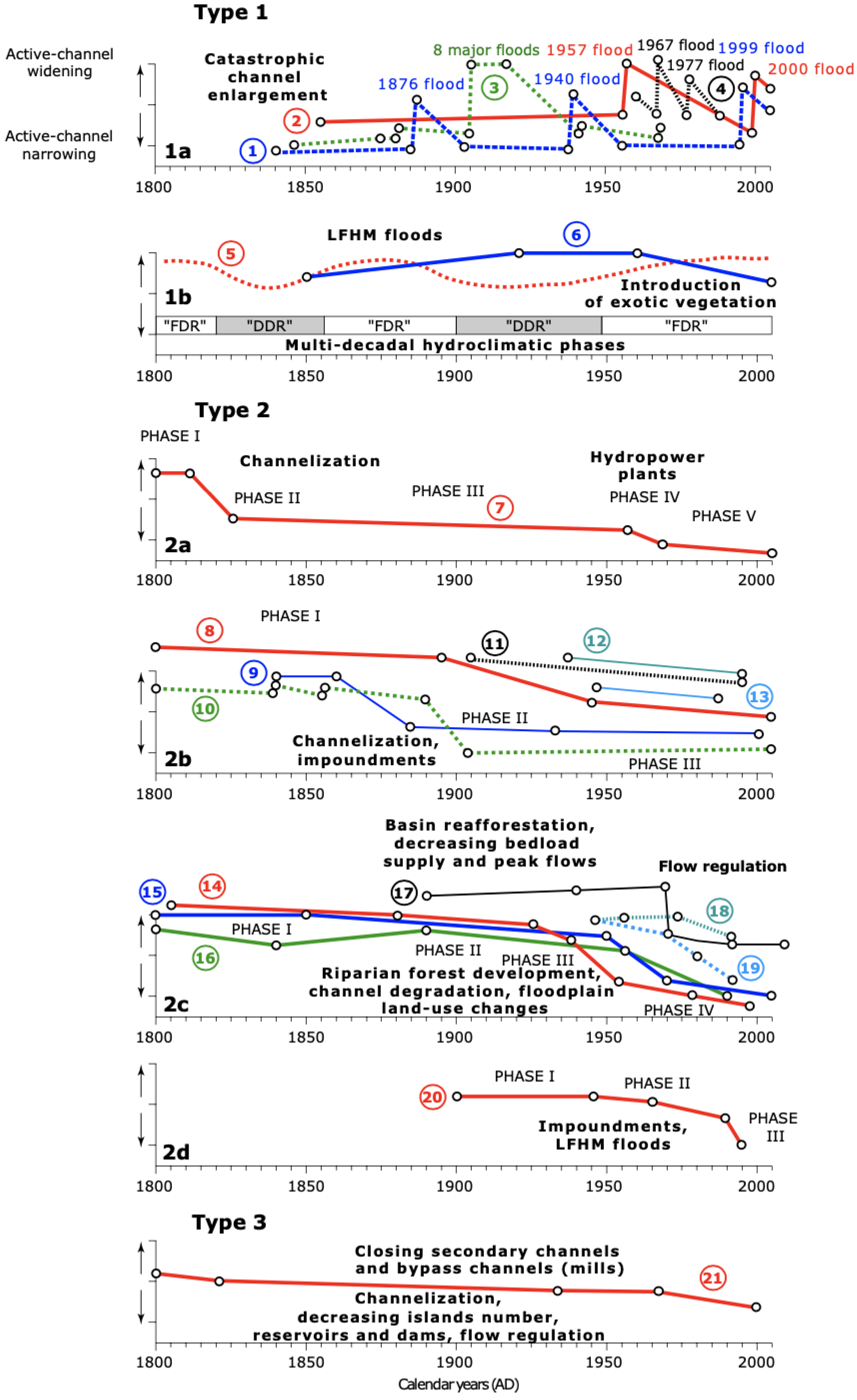
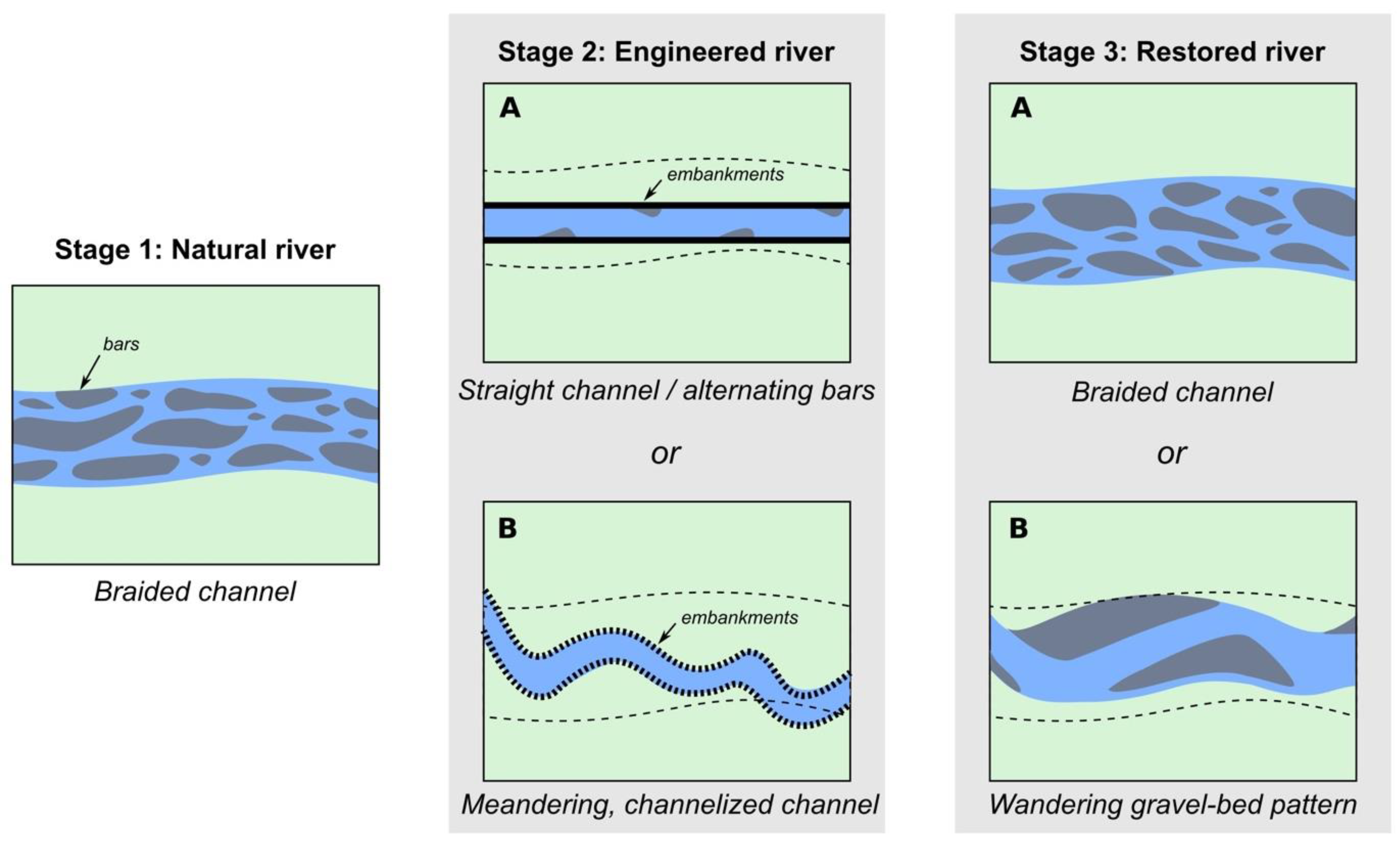
Stage 1: before significant functionalization of rivers. This stage can be assimilated to the free-flowing state of rivers (generally, before the eighteenth–nineteenth century, but sometimes before the Modern Times or Middle Ages). Lengthening or shortening of active channels by variations of fluvial style due to allocyclic and/or autocyclic processes is (i) common in high-energy rivers, (ii) much less in low-energy rivers.
-
Stage 2: before embankment removal associated with river restoration. (i) In the natural context (not constricted), high-energy rivers show a good ability to lengthen/shorten their multiple or single channels. In low-energy rivers, channel lengthening/shortening is possible but limited. (ii) In the artificialized context (channelized), no significant channel lengthening/shortening is possible either in high-energy rivers or in low-energy rivers.
-
Stage 3 (since 2000 with the emergence of environmental policies such as WFD in Europe that encourages restoration works [27,33,34]: current embankment removal accompanying river restoration. (i) In a natural context (not constricted), high-energy rivers are able to lengthen/shorten their multiple or single channels. Low-energy rivers can also be characterized by small channel lengthening/shortening when this occurs. (ii) In an artificialized context (channelized), high-energy rivers are exposed to a possible lengthening/shortening of their multiple or single channels. Low-energy rivers encounter high difficulty in lengthening/shortening their channel, and morphological adjustments are only locally visible.
This evolution, which tends towards a possible increase in the rate of lengthening/shortening of rivers in Stage 3, raises questions about how to take into account the longitudinal deformation of the multiple and single channels in the high-frequency monitoring of river beds from imagery. Surprisingly, the critical analysis of the literature concludes that the problem of longitudinal deformation of river beds (Figure 3) has not been taken into account in the story that is told from diachronic image processing.
In addition, if current trend is towards embankment removal, rivers are confronted with two situations (S), depending on their degree of energy expressed as ω = specific stream power [35,36,37]: (S1) rivers with sufficient energy (ω > 30 W/m2) allow moderate (30 W/m2 < ω < 100 W/m2) or significant (ω > 100 W/m2) geomorphological adjustments. (S2) rivers that have low energy (ω < 30 W/m2) allow nothing (ω < 10 W/m2) or not much (10 W/m2 < ω < 30 W/m2) in terms of geomorphological readjustments. We can cite in this regard the work of [28] on the Yerres River, a right-bank tributary of the Seine River upstream from Paris, which demonstrated during the 100-year R.I. flood (June 2016) that the river (ω < 30 W/m2) experienced no longitudinal and lateral change, with barely a few minor traces of weak incision in the channel bottom. The correlation of these two situations (S1, S2) with the new context of (i) embankment removal of rivers and (ii) the monitoring of the geomorphological impact of rivers restoration leads to improving the mapping method of fluvial beds, the subject of this paper.
The methods commonly used to analyze the temporal evolution of river channels from imagery, such as aerial photos and satellite images (2D variability), or even DTMs (e.g., BD Alti in France) and LIDAR surveys (3D variability), are based on transects (cross-sections) or channel-area calculation [38]. These cross-sections must meet two conditions: (i) they must always be perpendicular to the flow axis of the river; (ii) they must be equidistant, and this equidistance must not be modified to be reproducible, i.e., the measurements from one image to another must always be made at the same place. The variables drawn from the comparison of cross-sections are the channel width, braiding index, bed morphology, bed-material grain size, ecological habitat and the infrastructures located along the river channel and its margins [3]. In the case of the channel-area calculation, the ability of the stream to lengthen or shorten is neglected since what matters is the variation in the surface of the active channel over time. In any case, none of these methods currently allows taking into account the longitudinal and lateral deformation of rivers linked to the lengthening or shortening of their watercourse. These methods even become unsuitable when they lead to compare cross-sections that are not of the same number and not localized in the same place (Figure 3). Furthermore, very few studies [39,40,41,42,43] based on imagery, such as bathymetric maps or, recently, LIDAR data, report vertical shifts of the river channels and slope modification. Clearly, studies based on LIDAR data tend to provide deliverables such as sediment budgets, none of which offers methods to follow the planform dynamics of the river over an annual time step in the framework of river restoration.
The problematics of the paper are as follows: as long as the rivers were artificially constricted by an embankment (Figure 2, Stage 2), no lengthening or shortening of their watercourse was possible. From the moment the embankment removal occurred, lengthening or shortening of the rivers, driven by a change of river style, or quite simply by the revitalization of the river, asks to renew the diachronic mapping method derived from the imagery. While this may have had little impact on long-term studies and at the watershed scale, ‘classic’ methodology (i.e., based on diachronic cross-section analysis), which does not take into account the possible lengthening/shortening of the watercourse over time (Figure 3), is problematic in the case of detailed, operational studies carried out at the scale of the fluvial sectors. The objective of this paper is to draw up a protocol for analyzing images in fluvial geomorphology as part of river restoration so as to take into account the possible longitudinal deformation of the river channels through time.

2. Proposed Methodology

The methodological protocol developed in this paper proposes new indicators and a metric analysis grid to quantify the geomorphological changes occurring in rivers on an annual or multiannual scale. All these treatments can easily be completed by using GIS, such as QGIS open-source software, for instance [44].

2.1. The Purpose of New Indicators

We propose three new indicators. These three indicators allow quantifying distances between any points of a given active channel and any point within the adjacent watershed with different points of view (Figure 4): indicator 1: calculation of the distance between any points of the active channel and any point within the adjacent floodplain (Figure 4A,B); indicator 2: calculation of the distance between any points within the floodplain and the active channel (Figure 4C); indicator 3: calculation of the distance between any points of the active channel at one date and the same active channel at one other date (Figure 4D).
Note that the first indicator may be modified according to our goal. (i) If we are interested in the fluvial dynamics, we may calculate the distances between any points of the active channel and the margins of the floodplain (Figure 4A). By following this procedure for different dates, we can quantify the lateral migration of the active channel within the floodplain. (ii) If we are interested in fluvial risk management, with this first indicator, we may calculate the distance between any points of the active channel and any infrastructure built within the floodplain (Figure 4B).

2.1.1. Data Preparation

(i) Required Data. The calculation of the three indicators necessitates both spatial and temporal high-resolution images following regular monitoring. These images may be orthophotographs or very high-resolution satellite images. These images have to be georeferenced in a metric coordinate reference system such as UTM or any other national metric coordinate reference system.
(ii) Digitizing of the Active Channels. It is important to follow some basic rules when digitizing the active channels, which should be manually digitized as lines. The lines should be digitized at the middle of the active channel as it appears on the georeferenced images. In the case of large rivers (>30 m), it may be better to digitize rivers as surface and then calculate the centerline of this surface using GIS tools (such as «geometric attributes» in QGIS). The digitizing has to be completed from upstream to downstream. In the case the river is divided into multiple channels, such as braided rivers, it is better to digitize each channel individually. At this point, it is possible to digitize the active channels at different dates if the data are available. With this temporal dimension, it will be possible to follow the planform fluvial dynamics through time and the evolution of the hydrological risk. After the digitizing of the active channels, the lines should be converted to points. Indeed, the three indicators we develop require working with points and not directly with lines. We propose to extract a point for each meter along the active channel. For example, the plugin ‘interpolate point on line’ in QGIS allows us to extract regularly spaced points along a polyline in a very simple way.
(iii) Digitizing of the Floodplain Items. It is possible to digitize any items of interest (e.g., structures; riparian forest; urbanized, recreation or agricultural areas). In the case we are interested in fluvial dynamics, we may digitize the boundaries of the floodplain. These boundaries should only be the margins both of the right and left banks of the floodplain. In the case we are interested in risk management, we can digitize the infrastructure we want to protect. This infrastructure may be digitized as a point, a line or a polygon. However, if the infrastructure is first digitized as a line or a polygon, it should then be converted to points using the QGIS tool ‘polygon to line’, for instance. Then, regular points should be extracted from this line. We propose to extract a point every meter along the line or at the edge of the polygon of the infrastructure.

2.1.2. The Indicators

Figure 5 shows the workflow for the calculation of the three indicators.
(i) Indicator 1: Distance from Active Channel to Stakes or Floodplain Margins. This first indicator calculates the distance between any points of the active channel and any point within the floodplain. In order to quantify the temporal river dynamics, it is possible to calculate the distance between any points of the active channel and the floodplain boundaries. Thanks to this indicator, we can follow and quantify the lateral migrations of the active channels through time. The first step to build this indicator is to generate a raster proximity map indicating the distance from the center of each pixel to the floodplain boundaries. This may be completed by using the GDAL tool ‘gdal_proximity.py’ [45] interfaced in QGIS in the Raster menu ‘Proximity (Raster Distance’). The spatial resolution of this raster should be high. We recommend setting it to 1 m in order to be consistent with the points we have previously extracted along the active channel. Moreover, 1 m is an acceptable resolution because the active channels widen during floods and contract in between by much more, often by several tens of meters. This is what has been shown, for example, by the diachronic analysis of active channels in the French Southern Alps (Guil River) and on the foothills of the Montagne Noire (rivers Argent Double, Ognon and Clamoux; [46]). On this raster, the pixel values correspond to the distance between the pixel and the margins of the floodplain. For instance, a pixel with a value of 10 means that this pixel is 10 m away from the closest margin of the floodplain. The second step is to sample the value of this raster proximity map for each extracted point of the streams. In QGIS, we may use the ‘sample raster values’ tool. By performing this action, we know how far each point of the active channel is to the closest margin of the floodplain. In the case that we have the position of the river at different dates, we can quantify the lateral migration of the active channel.
From a perspective of risk management, we should now generate a raster proximity map indicating the distance from the center of each pixel to the infrastructure we want to protect in the floodplain. In this raster, the pixel values correspond to the distance between the pixel and the closest edge of the infrastructure to be protected. For instance, a pixel with a value of 10 means that this pixel is 10 m away from the closest edge of the infrastructure. Thanks to this indicator, it is possible to precisely identify the portions of the river which are less than a certain distance to the infrastructure. This indicator may help the river manager to identify the places where the building of embankments along the active channel can be relevant.
(ii) Indicator 2: Distance from Stakes to Active Channel. This indicator aims to calculate the distance between any points of the edges of any infrastructure and the active channel. It may help the river manager to precisely identify the places where it can be relevant to build a protection wall, for instance. The first step is to generate a raster proximity map indicating the distance from the center of each pixel to the channel. On this raster, the pixel values correspond to the distance between the pixel and the channel. For instance, a pixel with a value of 10 means that this pixel is 10 m away from the river. The second step is to sample the value of this raster proximity map for each point of the edges of the infrastructure. This indicator may help the manager to precisely identify which parts of the infrastructure should be protected. In the case that the position of the active channel is known for different dates, it is possible to follow the evolution of the vulnerability of the infrastructure through time.
(iii) Indicator 3: Diachronic Distance. This third indicator is used to quantify lateral migrations of the river through time. With this indicator, it is possible, for instance, to identify the sectors of the active channel which are highly unstable. This indicator is relevant only if at least two orthophotographs at two different dates are available. The first step is to choose one date as a reference. It may be the oldest one, for instance. Then, the raster proximity map indicating the distance from the center of each pixel to this reference channel should be generated. The second step is to sample the value of this raster proximity map for each extracted point of the channel of the second date. Finally, we obtain, for each point of the active channel of the second date, its distance to the active channel of the first date. A portion of active channel with a high distance means the river moved a lot in this sector. On the contrary, a portion of active channel with a low distance means the river did not move a lot in this sector.

2.2. The Metric Analysis Grid Approach

The analysis grid approach integrates the geographical variations of the active channel in the two-dimensional Euclidean space. After digitalization and georeferencing of the images, delimitation of the channel leads to manually digitize the riverbank boundaries as lines. The lines should be easily digitized when the riverbanks are not covered by tree vegetation. If the riparian forest or alluvial forest covers the riverbank, this creates a mask that does not allow us to see the edge of the river bank. After checking on the field (here, the Clamoux River), it turns out that the riverbanks can be delimited by passing by half of the first row of trees (semi-circles) bordering the active channel. Then, the study reach is rotated in order to obtain a rectangular area of investigation with a flow parallel to the X-axis as well as possible. A grid is created around the area of investigation with GIS software (for example, QGIS). The grid could be generated by vector calculation (with the QGIS ‘vector grid’ toolbox) or raster conversion (with the QGIS ‘vector to raster’ toolbox) with a sufficient resolution in comparison to the width/length of the studied reach. The resolution of the analysis grid is therefore the choice of the operator (Figure 6A). Here, we have chosen a metric analysis grid to follow the evolution of the two banks of the river between Year A and Year B in a 20 m × 40 m rectangular area of investigation. Each square (1 m × 1 m) occupied by the riverbank has been colored in red for the left bank and green for the right bank. Whatever the resolution choice, we recommend using an identical resolution for each survey of the monitoring.
The previous step of active-channel digitalization is used to characterize each grid cell by a specific code: 1 for the left bank, 2 for the right bank, 3 for the alluvial bar and 0 for all other objects (additional codes are possible to improve or complete the floodplain analysis by biological, hydrological, sediment or anthropogenic indicators). A classical selection by localization between the grid and geomorphological object (different riverbanks and alluvial bars) allows attributing the right code for each cell grid. The GIS database is then exported in a spreadsheet for different posttreatment as graphical output and indicator calculation. In order to avoid the case with more than one cell by column for the riverbank, the mean Y coordinate of the column is chosen to represent the unique Y coordinate of the column. The bank retreat/accretion is then calculated by the Y coordinate difference between Year B and Year A at each X unit. Careful attention is necessary to characterize the erosion or accretion in the function of the bank side and the flow direction. In our example, erosion of the left bank occurs for positive evolution, whereas accretion occurs for negative evolution and inversely for the right bank. Sometimes, the bank boundary passes through two superimposed squares. In this case, we take the average of the two squares for a diachronic comparison.
In the end, the evolution of the bank lines (or edge of the active channel) between Year A and Year B is reported on a histogram (Figure 6B) on which the measured bank sites (n = 40) are placed on the X-axis, and on the Y-axis, the values of erosion (bank retreat) or accumulation (bank accretion) for each of the two banks of the river. Reading the histogram of geomorphological adjustments of the channel between Year A and Yar B makes it possible to identify three types of river units: (i) units on which nothing is happening (no geomorphological change) between the two dates; (ii) units where there is a tendency to general retreat from the bank; (iii) and units where there is a tendency towards generalized accumulation. The entire histogram makes it possible to take into account both the lateral mobility of the channel as well as its longitudinal deformation. The difference in the number of alluvial-bar cells allows quantifying the longitudinal evolution of river deposits between Year A and Year B.
Regarding lateral mobility of the channel, we propose to apprehend it from a new indicator, i.e., the Lateral Mobility Rate (LMR; in %), expressed as:
LMR = ngc/n
where ngc is the number of sites having undergone geomorphological changes (bank retreat or bank accretion), and n is the total number of sites (or the number of cells counted in the bank edge). In the example chosen, LMR is equal to 28/40, or 70%, on the left bank, and 22/40, or 55%, on the right bank. In this case, the two banks are therefore mobile, and mobility is greater on the left bank (Table 2). The specific analysis of LMR by riverbank (left and right) makes it possible to see whether the river works more willingly on one of its banks or on both banks (and where possible, it will be necessary to voluntarily intervene and/or encourage the river to continue or to reduce its erosive activity).
It is then possible to calculate a sinuosity index and a braiding index. The sinuosity index (SI) is defined by [47] as the ‘channel length/straight-line valley length’ ratio. The braiding index (BI) corresponds to the average number of anabranches by section −1 [48]. In the proposed methodology, we adapted BI, which corresponds to the average number of anabranches by site −1 (here, n = 40).
One last clarification: the operator can choose to survey the values every meter, every 10 m, every 100 m, and so on. Therefore, the level of precision given to the study is the choice of the operator.

3. Applied Methodology
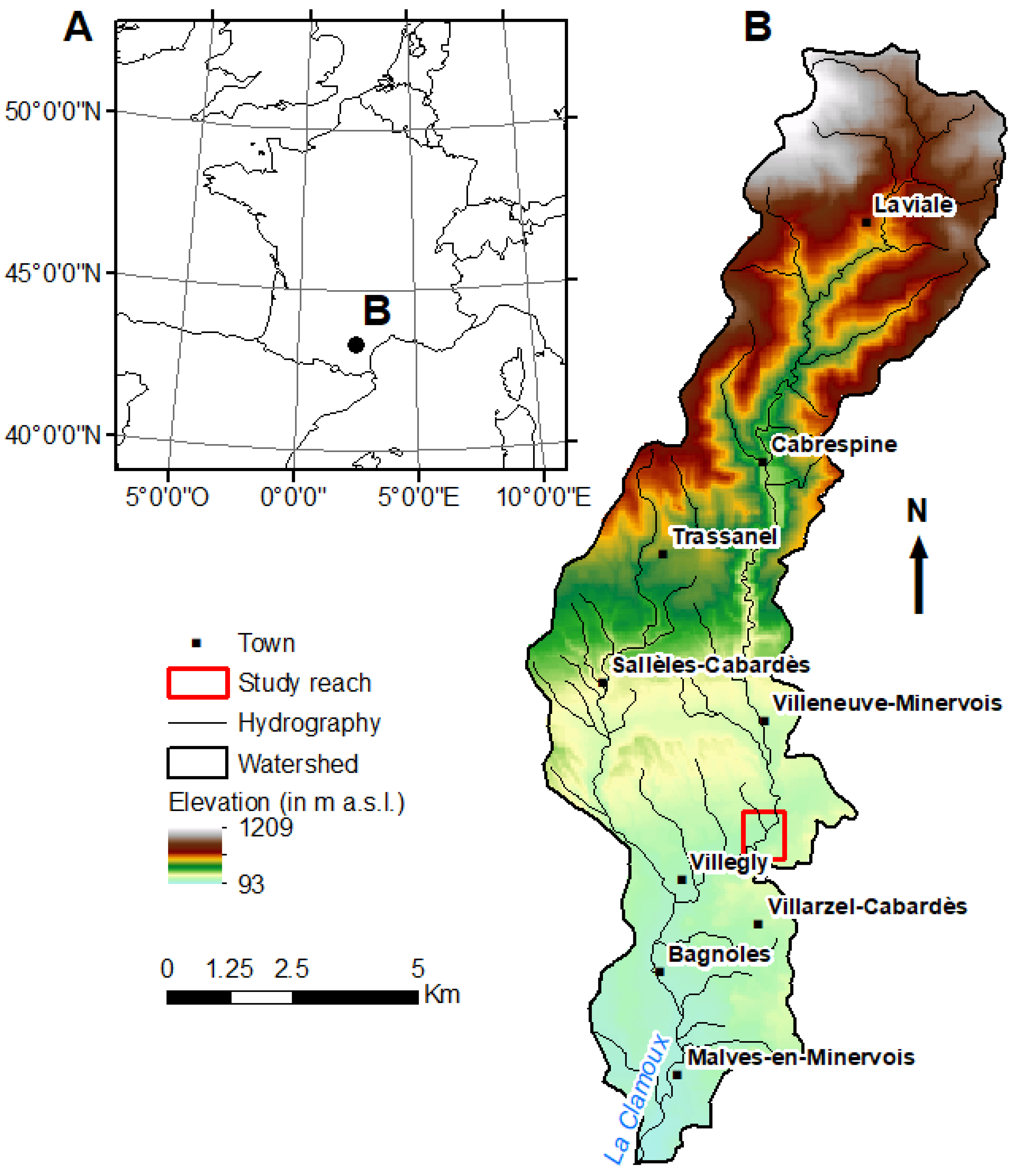
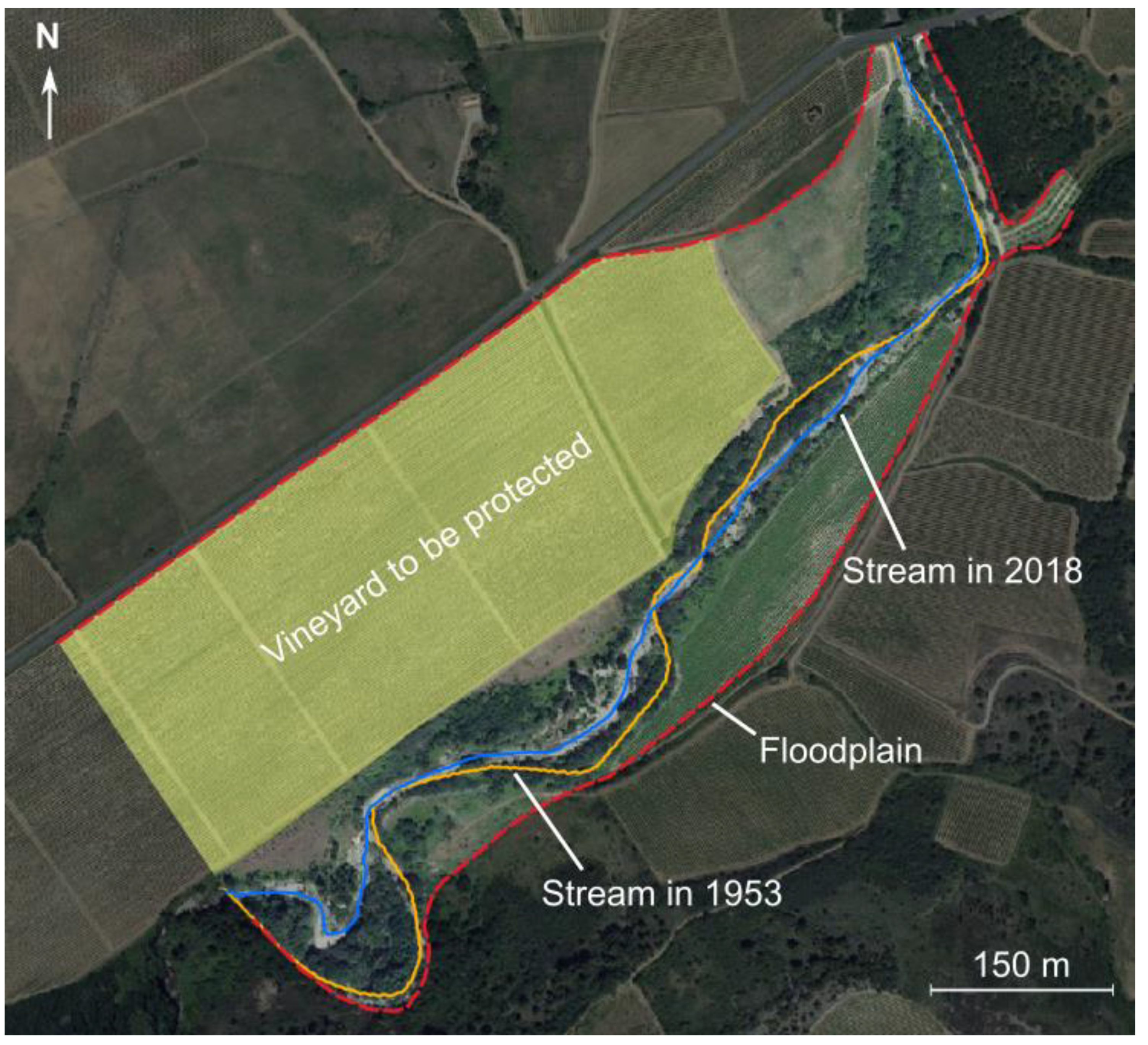
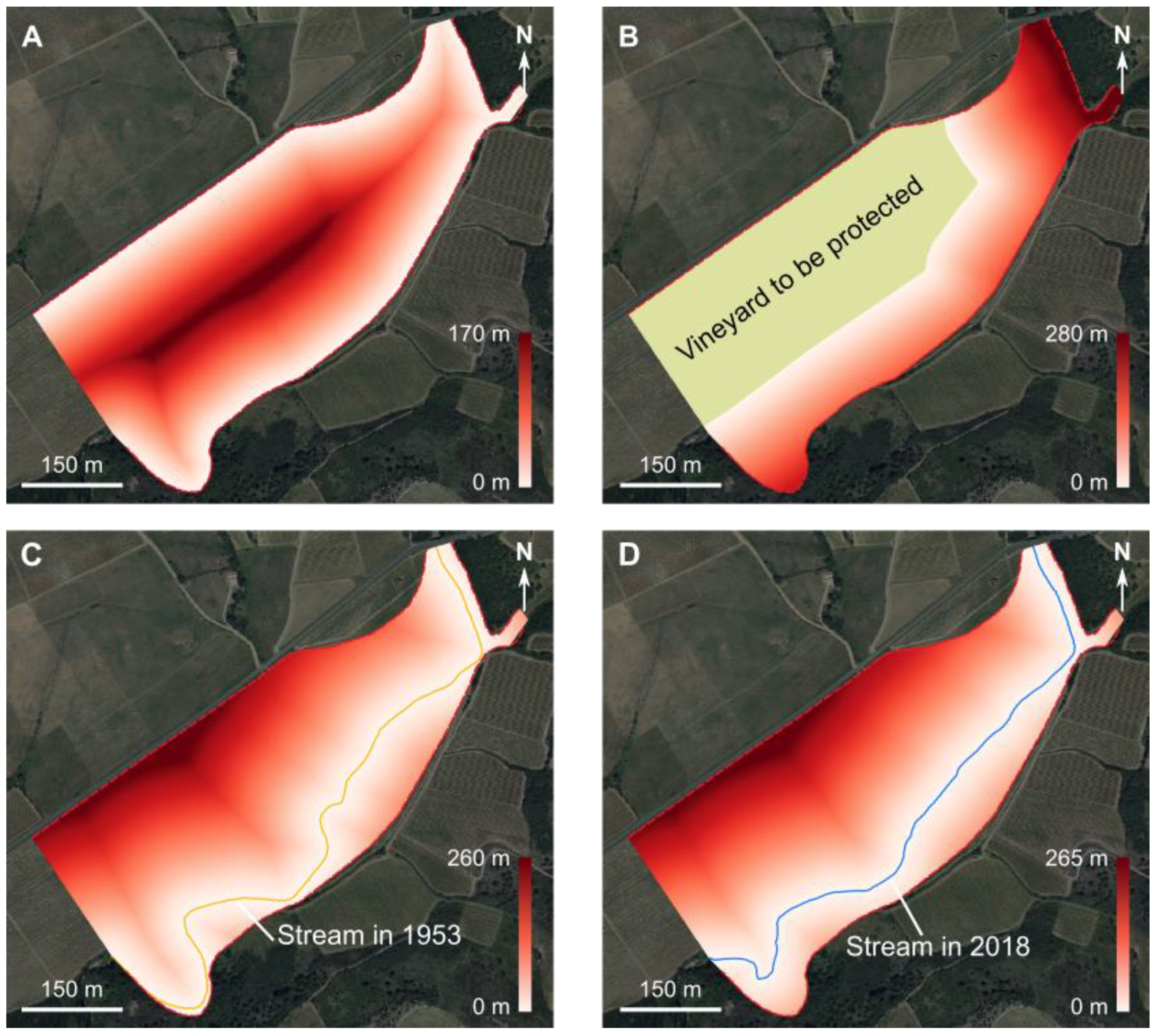
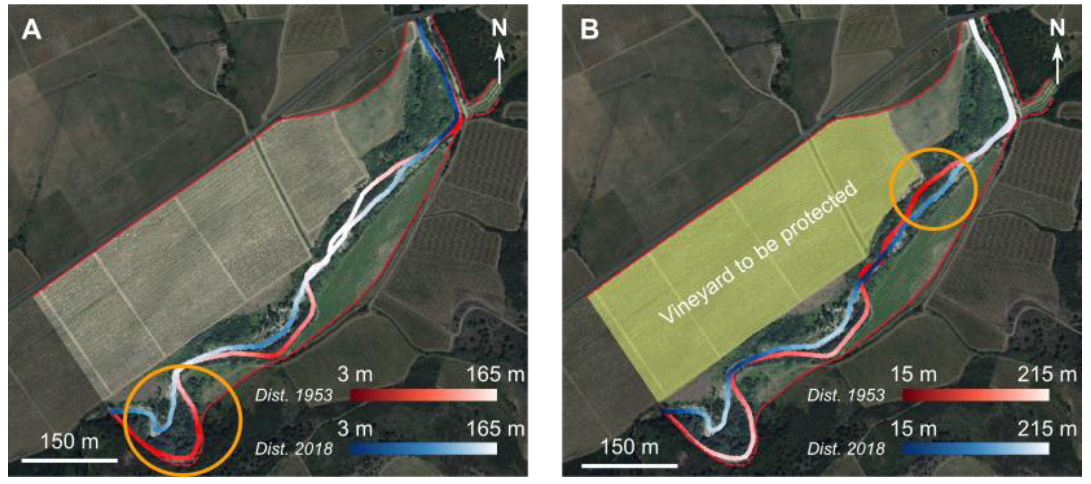
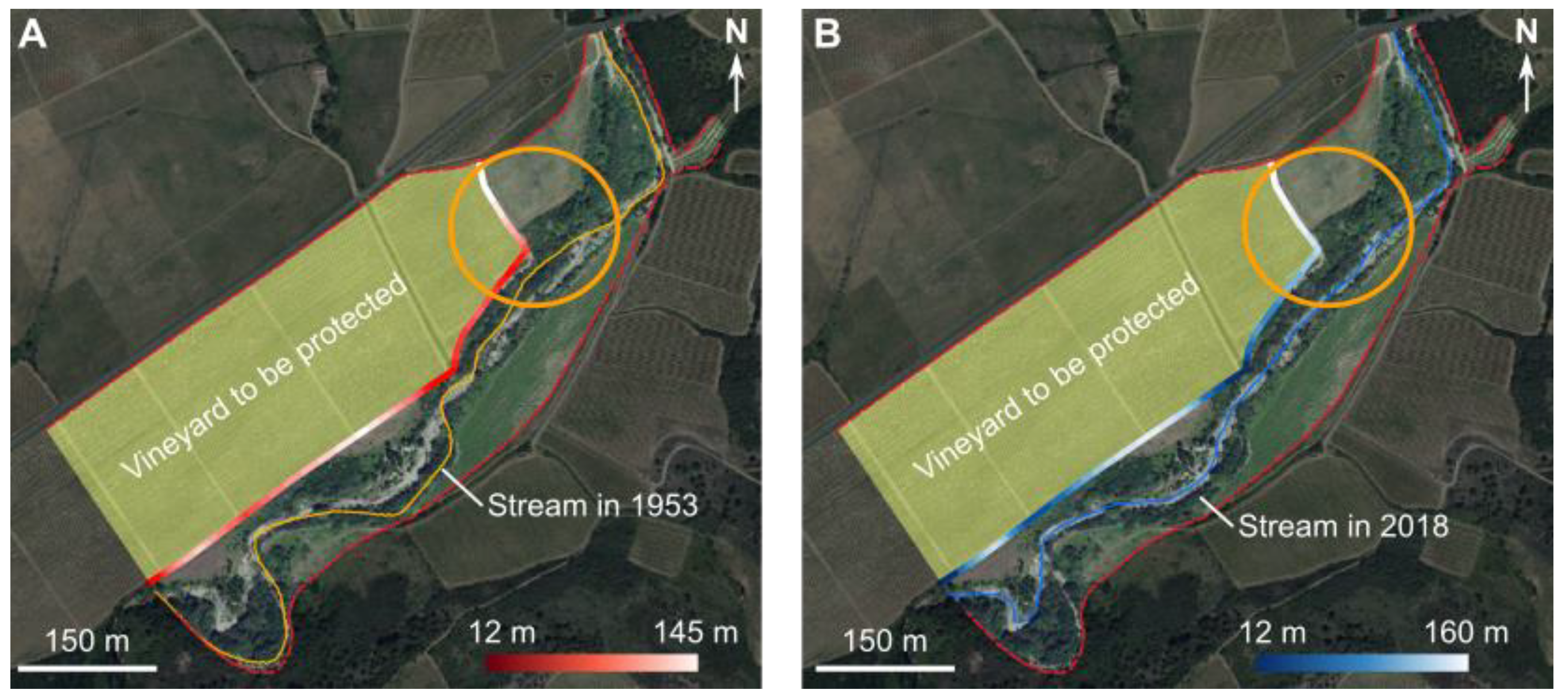
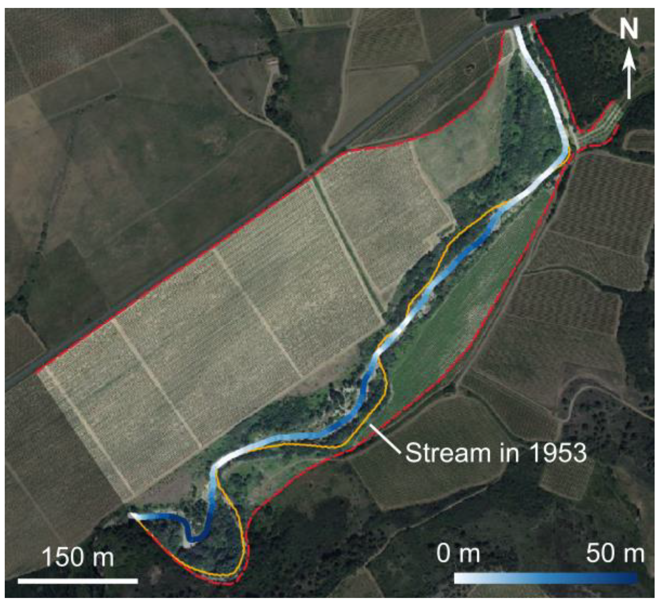
The case of low-energy single channels will not be developed in this paper because their low degree of evolution and slowness of morphological adjustments do not require that we modify the method classically used (i.e., diachronic analysis of equidistant cross-sections) to quantify the geomorphological evolution of the river channel. We will develop an example of a high-energy river characteristic of Mediterranean France. We show that the classic method (equidistant cross-sections) and the method proposed here do not lead at all to the same thing in terms of geomorphological monitoring and restitution of information to river managers. Below, we apply the proposed methodology to a river sector in a restoration context.

3.1. Study Area

We tested the ‘three indicators’ and the ‘metric grid approach’ in the Clamoux River, a left-bank tributary of the Orbiel River, which drains the Montagne Noire then the Minervois Piedmont in the Aude watershed (South of France; Figure 7). The Clamoux River (order 4, Strahler; length: 32.4 km; watershed area: 82 km2) is a confined, single-channel (plane bed or riffle pool) according to [49]. It was chosen as the test river for the proposed method for three main reasons. (i) It is a high-energy river, with a mean gradient of 3.2%, a Q100 1999 flood of 218 m3/s (for an annual mean discharge of 1 m3/s), which is typical of the intermittent Mediterranean river regime, with a bankfull, specific stream power of 280 W/m2 [2]. This high energy is explained by the boundary conditions of the watershed: high relief (1032 m; max. 1125 m–min. 93 m); Mediterranean climate favorable to flash floods from autumn to spring; the upstream part (mountain; schists) is marked by the rapid concentration (30 min) of water–sediment flows on the slopes (debris flows) and in the confined valley bottoms (hyper-concentrated flows); the downstream part (piedmont; molassic rocks) is characterized by water spreading and alluvial deposition in the floodplain when the river breaches its banks and structures, temporarily becoming a deconfined river. (ii) The Clamoux River experienced several extreme flash floods, including the November 1999 event (35 deaths in the South of France) and more recently, the February 2017 and October 2018 events. (iii) The Clamoux River has been the subject of restoration works since the creation in 2002 of the SMMAR—Syndicat mixte des milieux aquatiques et des rivières—the basin authority (EPTB) in charge of river management. These restoration works aim to let the river run its own course in zones where it has a tendency during each flood to bypass meanders (artificial channel pattern inherited from the seventeenth- to eighteenth-century embankments) and to open up new braided, active-channel segments. The SMMAR thus buys back the lands bordering the active channel from private owners. The goal is to control the river in its own freedom space, delimited by the stakes in the floodplain. The University of Paris/PRODIG Laboratory has been monitoring these restoration works on the field since the 1999 flood [1,2,50,51,52,53,54].
In the floodplain of the Clamoux River between the Aygadons Bridge and Villegly (Minervois piedmont), we digitized the active channel as it was in 1953, 2008 and 2018. This digitizing was carried out based on orthophotographs provided by the French Geographic Institute (IGN). The French national coordinate reference system (CRS) Lambert 93 (EPSG 2154) is used. It is a metric CRS. The floodplain boundaries were digitized based on field surveys and geological maps. A vineyard is located within the floodplain. In this example, this vineyard will be the infrastructure we want to protect (Figure 8).

3.2. Calculation of the Indicators

The starting point is to generate the different raster proximity maps. For indicator 1, from the perspective of fluvial dynamics study, the raster proximity map is calculated with the margins of the floodplain as the origin (Figure 9A). For indicator 1, from the perspective of risk management, the raster proximity map is calculated with the edges of the vineyard as origin (Figure 9B). For indicators 2 and 3, the raster proximity maps are generated using the location of the active channel in 1953 (Figure 9C) and in 2018 (Figure 9D).

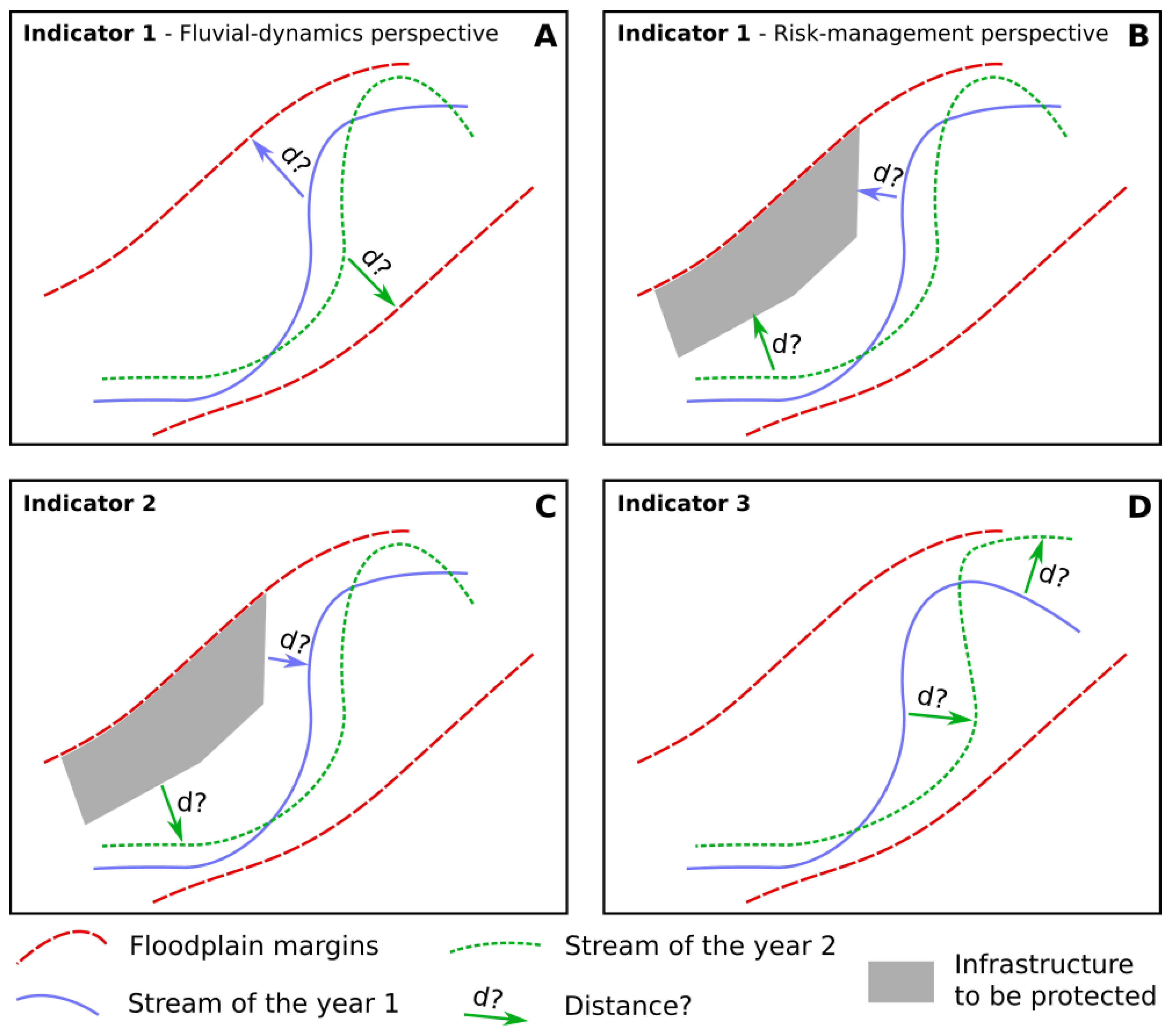
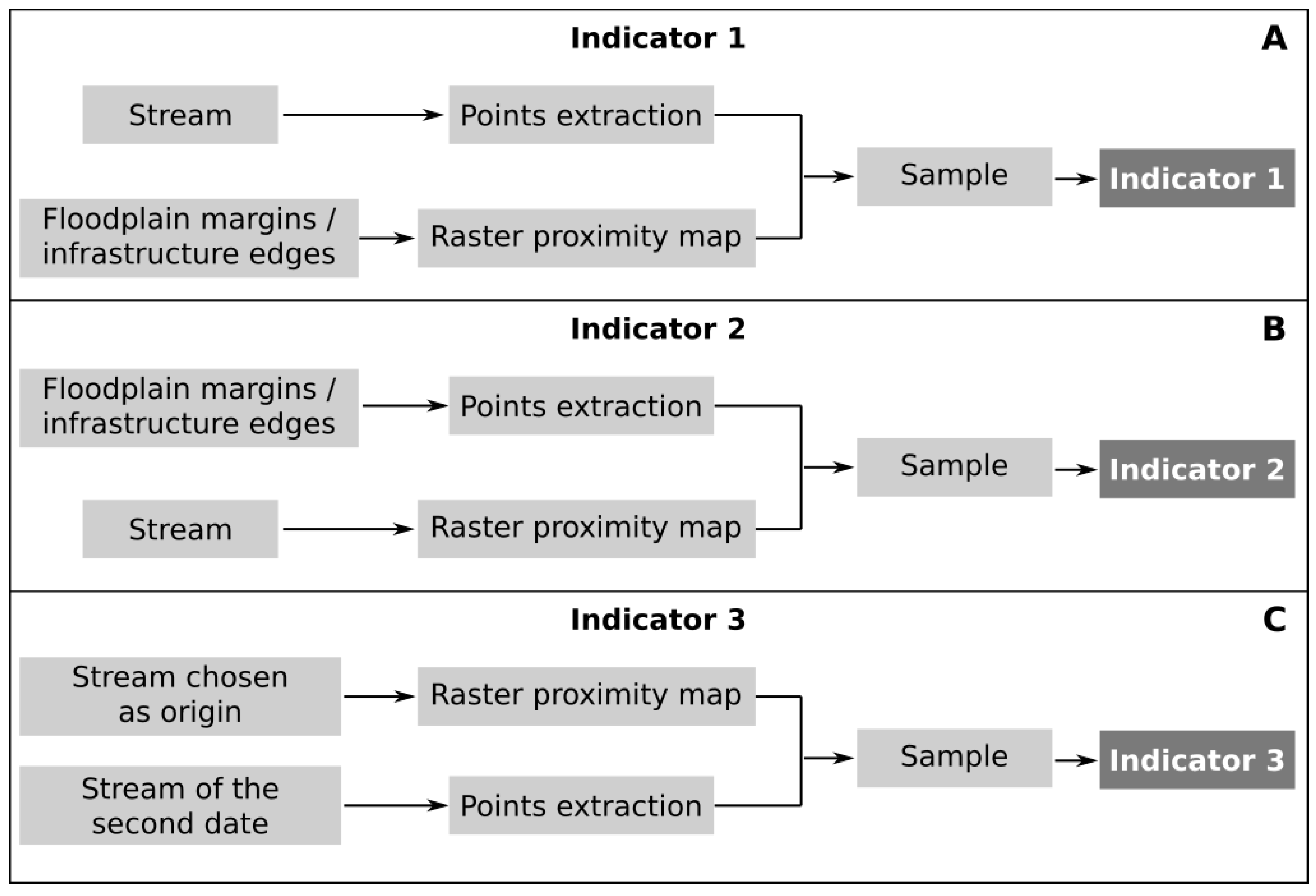
3.2.1. Indicator 1: Distance from Active Channel to Stakes or Floodplain Margins

From a perspective of fluvial dynamics study, we sample the extracted points of the active channels with the raster proximity map to the margins of the floodplain (Figure 9A). By performing this action, we may know how far each point of the channel to the margins of the floodplain is. This sampling is completed for the two dates. Finally, this version of indicator 1 gives information about the migration of the channel within the floodplain through time. For instance, in the highlighted sector in orange (Figure 10A), the channel was around 8 m away from the closest margin of the floodplain in 1953, but around 50 m away in 2018. Thus, this sector can be considered as unstable. On the contrary, the sectors that present the same distances values in both 1953 and 2018 can be considered as stable.
In a perspective of risk management, we sample the extracted points of the channels with the raster proximity map to the margins of the edges of the vineyard (Figure 9B). By performing this action, we may know how far each point of the channel is to the margins of the edges of the vineyard. This sampling is completed for the two dates. Finally, this version of indicator 1 shows the most actives sectors (in terms of bank erosion) of the channels for the vineyard and their evolution through time. This version of indicator 1 may help the river manager to identify the sectors where it could be relevant to build an embankment along the channel. In Figure 10B, on the highlighted sector in orange, in 1953, the channel was around 20 m away from the vineyard, and in 2018, it was around 50 m away. Thus, we can consider that the lateral dynamics of the river for the vineyard has decreased in this sector. If we have data relative to the elevation of the different items of the floodplain, we may better interpret this indicator by taking into account the elevation.

3.2.2. Indicator 2: Distance from Stakes to Active Channel

For the calculation of indicator 2, we sample the extracted points of the edges of the vineyard with the raster proximity map to the channels at the different dates (Figure 9C,D). By performing this action, we may know how far each point of the edges of the vineyard is to the channel. This sampling is completed for the two dates in order to follow the evolution of the vulnerability of the infrastructure through time (Figure 11). Figure 11A shows the distance between each point of the edges of the vineyard and the channel in 1953. Figure 11B shows the distance between each point of the edges of the vineyard and the channel of 2018. The edge of the vineyard in the highlighted sector in orange was around 20 m away from the channel in 1953 and around 50 m away in 2018. Thus, we can consider that this edge became less vulnerable through time. This indicator may help river managers to identify which part of the infrastructure has to be protected by embankments, for instance.

3.2.3. Indicator 3: Diachronic Distance

For the calculation of this indicator 3, one channel should be chosen as reference. The oldest one may be chosen, for instance. Once this channel is chosen, the raster proximity map to this channel is generated (Figure 9C). Then, we sample each extracted point of the 2018 channel with this raster proximity map. By performing this action, we may know how far each point of the channel of 2018 is from the 1953 channel. This indicator clearly shows stable and unstable sectors. In Figure 12, the blue sectors are the sectors which moved a lot between 1953 and 2018. On the contrary, the white sectors are the sectors which did not move a lot between these two dates. The bluest part of the 2018 channel indicates that the channel in this sector moved around 50 m between 1953 and 2018.

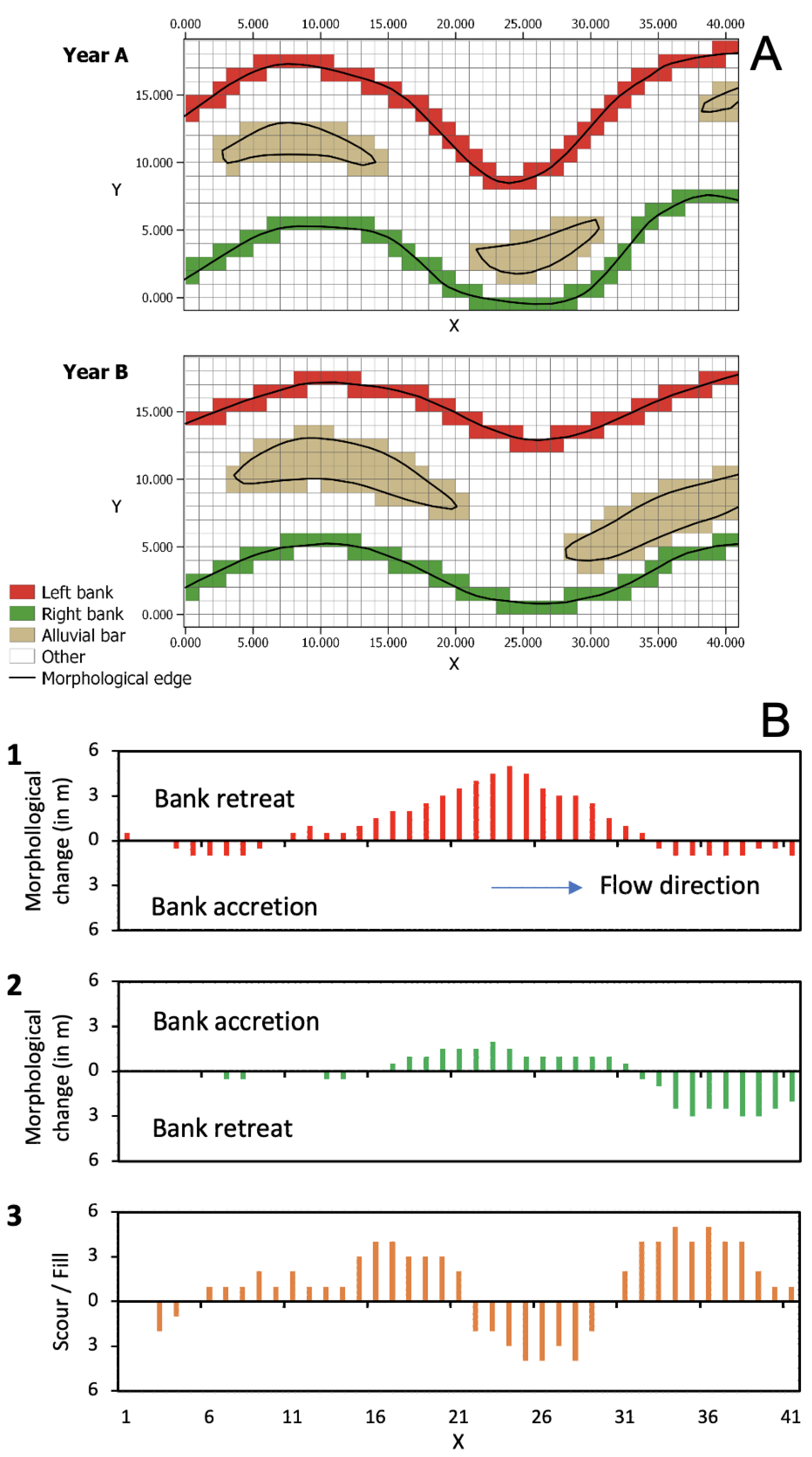
3.3. The Metric Analysis Grid Approach

The Metric Analysis Grid Approach focuses on a 250 m sub-reach of the Clamoux River. Grid resolution is fixed to 1 m2 and was rotated 30° from the initial area of investigation (Figure 13). Only bank retreat/bank accretion on the channel margins is quantified (and not the alluvial bars) because of the relatively poor spatial resolution of the image in comparison to the channel width and masked area by the riparian forest.
Between 2008 and 2018, our method shows a clear general bank migration to the left side of the active channel with bank retreat (7.3 m on average) in the left bank and bank accretion (6.4 m on average) in the right bank. LMR indicator (92% for the left bank and 98% for the right bank; Table 3) highlights the longitudinal magnitude of riverbank evolution, which is similar on both sides and close to a total bank reworking. Lateral mobility (LMR) is slightly lower on the left bank due to the blockage of the active channel against the Pleistocene alluvial terraces bordering the floodplain.
These channel dynamics are controlled by the flood of February 2017 (62.7 m3/s; >Q50), which is responsible for a strong geomorphological adjustment, characterized by channel widening over 40 m in the study reach, as shown by field observation of the right bank position in February 2017; Figure 13). Due to the rapid vegetation recolonization in the right bank, the active channel of the Clamoux River in 2018 (before the October flood event) is not as wide as the active channel during the February 2017 flood. This process explains why sinuosity is higher after a morphogenic flood event, reflecting the stabilization of hydrodynamic conditions.

4. Discussion

4.1. New Indicators

The proposed three new indicators may help the scientist and the river manager to better understand the local hydrosystem and its temporal dynamics. These indicators are deduced from a manually calculated centerline. We have tested the automatic extraction of the centerline: it is not at all relevant at the moment because any software does not always know how to place the cross-section perpendicular to the river flow axis. Thus, we spend more time correcting these errors than drawing the centerline manually. Hence, the choice to draw a centerline manually.
The version of the first indicator calculating the distance from the streams to the margins of the floodplain at different dates gives information about the lateral migrations of the channels within the floodplain through time. The stable and unstable sectors are clearly highlighted. The version of the first indicator calculating the distance from the streams to the stake at different dates highlights the potentially dangerous parts of the streams. This version of the indicator may help the river manager to precisely identify the sectors where it could be relevant to build an embankment along the channel.
The second indicator calculating the distance from the stake to the streams at different dates highlights the evolution of the vulnerability of the stake through time. With this indicator, the river manager may identify the most vulnerable parts of the stake in order to possibly build a protection wall, for instance.
The third indicator focuses on the fluvial dynamics of the local system. It is useful to quantify the lateral migrations of the channels between two dates. This indicator highlights the stable and the unstable sectors without any information about the floodplain.

4.2. The Metric Analysis Grid in the Two-Dimensional Euclidean Space

The analysis of river segments using the metric analysis grid allows us to properly quantify the river dynamics in space-time. Figure 13 shows the superior quality of the results obtained with the metric analysis grid, compared to what we would have obtained using cross-sections. As shown by the classical approach, in the case of the Clamoux River, cross-sections could not allow us to properly quantify bank dynamics because (i) mean active-channel width (W) variations are very weakly negative (W = −0.33 m), which does not at all reflect the bank dynamics (i.e., right bank accretion and left bank retreat) perceived by the metric grid analysis, and (ii) the critical sites for bank management are not captured.
This metric analysis grid is a dashboard that is useful not only for scientists but also for river managers. In fact, in a river-restoration context, we need fairly detailed monitoring of the geomorphological readjustments produced by the river subjected to new boundaries conditions (removal of lateral constraints, increase in the energy slope, the channel width and braided index, decrease of sinuosity index, reactivation of sediment transport and alluvial forest development).
We strongly recommend annual monitoring in the case of a dynamic river (ω > 30 W/m2) in addition to a survey after a significant flood event. It is therefore necessary to plan one to several overflights of the studied area (drone, plane) to obtain images (photos, LIDAR). Monitoring campaigns should not be held during the growing season in order to limit vegetation hold on images.
This metric analysis grid constitutes a simplified approach to the geomorphological reality. A grid with a metric resolution (i.e., the resolution chosen here) indeed makes it possible to perceive geomorphological changes (e.g., bank retreat, bar accretion) within the active channel greater than 1 m. As part of a braided, active channel without strong human and/or material stakes, we are not within a meter. If this is the case, we must move to an engineering-type approach. Anyway, the analysis resolution can be adjusted by the operator depending on the precision desired. The grid does not prevent finer measurements on erosion processes, but the advantage is to bring geographical (systemic) dimensions of the active-channel functioning here. This systemic vision is what managers expect from researchers.
This method based on the metric grid also has the advantage of being able to survey the river banks without using images. In fact, the bank lines can be first surveyed with a GPS and then subsequently transferred to the metric grid. It can even be considered to transfer all types of field observations (geomorphology, sediment, vegetation, structures) directly to the grid.
This method assumes a good knowledge of the field and geomorphological processes because rivers are systemic, and it is not enough to observe erosion or deposition in such sites rather than others: we have to know how to interpret and predict the future of the river segments at +5 or +10 years at least (ideally +50 years). Only the understanding of geomorphological processes makes it possible to interpret our metric analytical grid and its use in the future.
About the braided index, the work can be improved concerning the quantification of the number of alluvial bars. However, for river restoration, this may be enough to identify sediment storage areas. This will be very useful (i) to alert that a river segment is being infilled, favoring the water overflow (inundation) by reducing the channel capacity, or on the contrary, (ii) to reassure that the alluvial transport is effective with good longitudinal/lateral connections within the watershed and that alluvial transport is slowed down in river reaches where there are no stakes, in order to avoid sediment deposits, for example, in urban areas exposed to a strong inundation risk.

5. Conclusions

We consider this work to help overcome the big difficulty of river managers, which is the monitoring of the active channels and parameters to be retained for good hydro-bio-sedimentary functioning. In fact, river managers generally call on researchers to help them understand how a river unit behaves after restoration works (e.g., after embankment removal). The river, if it is dynamic (ω > 30–100 W/m2), will then be capable of significant morphological adjustments (lateral mobility by bank erosion or avulsion in terms of planform variations; channel incision/aggradation) in the year of several meters or even much more. However, the managers are field workers, and very few of them have time to map the morphological changes they observe each day along the river. Furthermore, they know how to interpret the morphological adjustments of the river when they occur on a case-by-case basis. However, there too, the forward-looking vision of the ‘new’ river left to its own devices makes it difficult for them. In short, managers need help from scientists. For their part, geomorphologists understand that it is possible to transcribe these changes by monitoring the river geometry. In this paper, we have proposed a new method, which integrates the possibility of taking into account the precise deformation (both lateral and longitudinal) of the active channel, having previously noted the biases of existing methods in the literature and in practice. The main contribution of the metric analysis grid in 2D Euclidean space (Section 2.2 and Section 3.3) is precisely to provide a geographical (systemic) dimension within the framework of the observation and measurement of erosion processes along rivers. The cross-section surveys are too limited and imprecise for this in that they give a too local and discontinuous view of the river, in addition to not allowing the longitudinal deformation of the channel to be taken into account in dynamic river systems. The comparison of river surfaces on the scale of the floodplain is of no interest to the river managers because they are too general; they do not quantify changes at the scale of the river segment, river reach and geomorphic units. The introduction of the three new indicators based on accessible and easily reproducible GIS technics brings quantification about the dynamics of the local hydrosystem. This semi-automatic procedure of quantification makes it easier to follow the evolution of the system through time. May this work allow researchers and managers to make a precise annual (or after an event) diagnosis of river functioning. The sectors where the river is dynamic will be identified well and monitored, and they may be the subject of special attention faced to the stakes in the floodplain, which must be defended more or less strongly according to their nature (human, material). We will also be able to better understand the trajectories of the hydrosystems by the high-resolution analysis and monitoring of sectors that are regularly exposed to erosion or deposition. The proposed indicators may go beyond river-restoration issues. What we have proposed is ultimately interesting for any dynamic river segment, whether it is being restored or not.

Author Contributions

Conceptualization, G.A.-F.; Methodology, G.A.-F. and P.P.; Software, P.P. and G.B.; Validation, G.A.-F., P.P., G.B. and G.M.; Formal Analysis, G.A.-F. and G.M.; Investigation, G.A.-F.; Resources, O.T.; Data Curation, G.A.-F. and P.P.; Writing—Original Draft Preparation, G.A.-F. and P.P. (Section 2.1, Section 3.2 and Section 4.1); Writing—Review and Editing, G.A.-F., P.P., G.B. and G.M.; Visualization, G.A.-F., P.P., G.B. and G.M.; Supervision, G.A.-F.; Project Administration, G.A.-F. All authors have read and agreed to the published version of the manuscript.

Funding

This research received no external funding.

Acknowledgments

The authors would like to thank the SMMAR, the SMAC, the ADREUC, the Agence de l’Eau and the OFB for their support of the research, and the four reviewers and the editorial board of the journal for their comments, which greatly helped to improve the first version of the manuscript.

Conflicts of Interest

The authors declare no conflict of interest.

References

  1. Arnaud-Fassetta, G.; Beltrando, G.; Fort, M.; Plet, A.; André, G.; Clément, D.; Dagan, M.; Méring, C.; Quisserne, D.; Rycx, Y. La catastrophe hydrologique de novembre 1999 dans le bassin-versant de l’Argent Double (Aude, France): De l’aléa pluviométrique à la gestion des risques pluviaux et fluviaux. Géomorphol. Relief Process. Environ. 2002, 8, 17–34. [Google Scholar] [CrossRef]
  2. Brousse, G. Efficacité des Travaux de Restauration et Résilience des Rivières Torrentielles Altérées. Ph.D. Thesis, University of Paris, Paris, France, 2020. [Google Scholar]
  3. Arnaud-Fassetta, G.; Fort, M. Hydro-bio-morphological changes and control factors of an upper Alpine valley bottom since the mid-19th century. Case study of the Guil River, Durance catchment, southern French Alps. Méditerranée 2014, 122, 159–182. [Google Scholar] [CrossRef]
  4. Brousse, G.; Arnaud-Fassetta, G.; Cordier, S. Évolution hydrogéomorphologique de la bande active de l’Ubaye (Alpes françaises du Sud) de 1956 à 2004: Contribution à la gestion des crues. Géomorphol. Relief Process. Environ. 2011, 17, 307–318. [Google Scholar] [CrossRef] [Green Version]
  5. Burkham, D.E. Channel Changes of the Gila River in Safford Valley, Arizona, 1846–1970; Professional Paper 655-G; US Geological Survey: Washington, DC, USA, 1972; 24p. [Google Scholar]
  6. Yu, B. The hydrological and geomorphological impacts of the Tinaroo Falls Dam on the Barron River, North Queensland, Australia. In River Management. The Australasian Experience; Brizga, S., Finlayson, B., Eds.; Wiley: Chichester, UK, 2000; pp. 73–95. [Google Scholar]
  7. Erskine, W.D.; Warner, R.F. Geomorphic effects of alternating flood and drought dominated regimes on NSW coastal rivers. In Fluvial Geomorphology of Australia; Warner, R.F., Ed.; Academic Press: Sydney, Australia, 1988; pp. 223–244. [Google Scholar]
  8. Brooks, A.P.; Brierley, G.J. The role of European disturbance in the metamorphosis of the lower Bega River. In River Management. The Australasian Experience; Brizga, S., Finlayson, B., Eds.; Wiley: Chichester, UK, 2000; pp. 221–246. [Google Scholar]
  9. Hohensinner, S.; Habersack, H.; Jungwirth, M.; Zauner, G. Reconstruction of the characteristics of a natural alluvial river-floodplain system and hydromorphological changes following human modifications: The Danube River (1812–1991). River Res. Appl. 2004, 20, 25–41. [Google Scholar] [CrossRef]
  10. Miramont, C.; Jorda, M.; Pichard, G. Évolution historique de la morphogenèse et de la dynamique fluviale d’une rivière méditerranéenne: l’exemple de la Moyenne Durance (France du Sud-est). Géogr. Phys. Quat. 1998, 52, 381–392. [Google Scholar] [CrossRef] [Green Version]
  11. Laigre, L.; Arnaud-Fassetta, G.; Reynard, E. Cartographie sectorielle du paléoenvironnement de la plaine alluviale du Rhône suisse depuis la fin du Petit Âge Glaciaire: La métamorphose fluviale de Viège à Rarogne et de Sierre à Sion. Bull. Murithienne 2009, 127, 7–17. [Google Scholar]
  12. Arnaud-Fassetta, G. River channel changes in the Rhone Delta (France) since the end of the Little Ice Age: Geomorphological adjustment to hydroclimatic change and natural resource management. Catena 2003, 51, 141–172. [Google Scholar] [CrossRef]
  13. Bravard, J.-P.; Provansal, M.; Arnaud-Fassetta, G.; Chabbert, S.; Gaydou, P.; Dufour, S.; Richard, F.; Valleteau, S.; Melun, G.; Passy, P. Un atlas du paléo-environnement de la plaine alluviale du Rhône de la frontière suisse à la mer. Édytem 2008, 6, 101–116. [Google Scholar] [CrossRef]
  14. Cubizolle, H. La morphodynamique fluviale dans ses rapports avec les aménagements hydrauliques: l’exemple de la Dore au XXe siècle (Massif Central, France). Géomorphol. Relief Process. Environ. 1996, 1, 67–82. [Google Scholar] [CrossRef]
  15. Peiry, J.-L.; Pupier, N. La notion de lit fluvial sur les rivières alpines et méditerranéennes et ses implications pour la gestion du chenal. Études Vauclus. 1994, 5, 51–57. [Google Scholar]
  16. Gautier, E.; Piégay, H.; Bertaina, P. A methodological approach of fluvial dynamics oriented towards hydrosystem management: Case study of the Loire and Allier rivers. Geodin. Acta 2000, 1, 29–43. [Google Scholar] [CrossRef] [Green Version]
  17. Peiry, J.-L.; Nouguier, F. Le Drac dans l’agglomération de Grenoble: Première évaluation des changements géomorphologiques contemporains. Rev. Géogr. Alp. 1994, 2, 77–96. [Google Scholar] [CrossRef]
  18. Liébault, F.; Piégay, H. Causes of 20th century channel narrowing in mountain and piedmont rivers of southeastern France. Earth Surf. Process. Landf. 2002, 27, 425–444. [Google Scholar] [CrossRef]
  19. Siché, I.; Arnaud-Fassetta, G. Anthropogenic actions since the end of the Little Ice Age: A critical factor controlling the last ‘fluvial metamorphosis’ of the Isonzo River (Italy, Slovenia). Méditerranée 2014, 122, 183–200. [Google Scholar] [CrossRef] [Green Version]
  20. Descroix, L.; Gautier, E. Water erosion in the southern French alps: Climatic and human mechanisms. Catena 2002, 50, 53–85. [Google Scholar] [CrossRef]
  21. Salit, F.; Arnaud-Fassetta, G.; Zaharia, L.; Madelin, M.; Beltrando, G. The influence of river training on channel changes during the 20th century in the Lower Siret River, Danube catchment (Romania). Géomorphol. Relief Process. Environ. 2015, 21, 175–188. [Google Scholar] [CrossRef]
  22. Brierley, G.J.; Fitchett, K. Channel planform adjustments along the Waiau River, 1946-1992: Assessment of the impacts of flow regulation. In River Management. The Australasian Experience; Brizga, S., Finlayson, B., Eds.; Wiley: Chichester, UK, 2000; pp. 51–71. [Google Scholar]
  23. Piégay, H.; Salvador, P.-G.; Astrade, L. Réflexions relatives à la variabilité spatiale de la mosaïque fluviale à l’échelle du tronçon. Z. Für Geomorphol. 2000, 44, 317–342. [Google Scholar]
  24. Gilvear, D.J. Patterns of channel adjustment to impoundment of the upper River Spey, Scotland(1942–2000). River Res. Appl. 2003, 20, 151–165. [Google Scholar] [CrossRef]
  25. Lescure, S.; Arnaud-Fassetta, G.; Cordier, S. Sur quelques modifications hydromorphologiques dans le Val de Seine (Bassin parisien, France) depuis 1830: Quelle part accorder aux facteurs hydrologiques et anthropiques? EchoGeo 2011, 18, 15. [Google Scholar] [CrossRef] [Green Version]
  26. Alaoui, K. Les Modifications Hydro-Morphodynamiques dans la Plaine Alluviale aval de l’Yerres Sous L’influence de L’anthropisation. Master’s Thesis, University Denis-Diderot, Paris, France, 2000. [Google Scholar]
  27. Melun, G. Impacts Environnementaux de la Suppression des Ouvrages Hydrauliques dans le Cadre du Rétablissement de la Continuité des Cours D’eau Imposée par la Loi sur L’eau et les Milieux Aquatiques. Ph.D. Thesis, University Paris-Diderot, Paris, France, 2012. [Google Scholar]
  28. Michler, L. Impacts Hydromorphologiques et Sédimentaires du Décloisonnement de l’Yerres. Identification, Quantification, Spatialisation. Ph.D. Thesis, University Paris-Diderot, Paris, France, 2018. [Google Scholar]
  29. Bennett, S.J.; Simon, A.; Castro, J.M.; Atkinson, J.F.; Bronner, C.E.; Blersch, S.S.; Rabideau, A.J. The evolving science of stream restoration. In Stream Restoration in Dynamic Fluvial Systems: Scientific Approaches, Analyses, and Tools; Geophysical, Monograph; Simon, A., Bennett, S.J., Castro, J.M., Eds.; American Geophysical Union: Washington, DC, USA, 2011; Volume 194, pp. 1–8. [Google Scholar]
  30. Wohl, E.; Lane, S.N.; Wilcox, A.C. The science and practice of river restoration. Water Resour. Res. 2015, 51, 5974–5997. [Google Scholar] [CrossRef] [Green Version]
  31. Morandi, B.; Piégay, H. La Restauration des Cours d’eau en France: Comment les Définitions et les Pratiques Ont-Elles Evolué Dans le Temps et Dans L’espace, Quelles Pistes D’action Pour le Futur? Agence Française pour la Biodiversité, Collection Comprendre pour agir: Paris, France, 2017; 28p. [Google Scholar]
  32. Malavoi, J.-P.; Bravard, J.-P.; Piégay, H.; Heroin, E.; Ramez, P. Détermination de L’espace de Liberté des Cours D’eau, SDAGE Rhône Méditerranée Corse, Guide Technique 2; France. 1998; 42p.
  33. Dufour, S.; Piégay, H. From the myth of a lost paradise to targeted river restoration: Forget natural references and focus on human benefits. River Res. Appl. 2009, 25, 568–581. [Google Scholar] [CrossRef]
  34. Morandi, B. La Restauration des Cours d’eau en France et à L’étranger: De la Définition du Concept à L’évaluation de L’action. Éléments de Recherche Applicables. Ph.D. Thesis, ENS Lyon, Lyon, France, 2014. [Google Scholar]
  35. Brookes, A. Channelized Rivers: Perspectives for Environmental Management; Wiley: Chichester, UK, 1988; 342p. [Google Scholar]
  36. Wasson, J.-G.; Malavoi, J.-R.; Maridet, L.; Souchon, Y.; Paulin, L. Impacts Ecologiques de la Chenalisation des Rivières; CEMAGREF Éditions, Collection «Études», Gestion des Milieux Aquatiques 14; CEMAGREF: Antony, France, 1998; 158p. [Google Scholar]
  37. Adam, P.; Debiais, N.; Malavoi, J.-R. Manuel de Restauration Hydromorphologique des Cours D’eau; Agence de l’eau Seine Normandie: Nanterre, France, 2007; 62p. [Google Scholar]
  38. Kondolf, M.G.; Piégay, H. Tools in Fluvial Geomorphology; Wiley: Chichester, UK, 2003; 696p. [Google Scholar]
  39. Lallias-Tacon, S. Analyse Spatio-Temporelle de la Morphologie des Rivières en Tresses par LiDAR Aéroporté. Ph.D. Thesis, University Lyon 2, Lyon, France, 2015. [Google Scholar]
  40. Michez, A.; Piégay, H.; Lejeune, P.; Claessens, H. Multi-temporal monitoring of a regional riparian buffer network (>12,000 km) with LiDAR and photogrammetric point clouds. J. Environ. Manag. 2017, 202, 424–436. [Google Scholar] [CrossRef]
  41. Bizzi, S.; Piégay, H.; Demarchi, L.; van de Bund, W.; Weissteiner, C.J.; Gob, F. LiDAR-based fluvial remote sensing to assess 50-100-year human-driven channel changes at a regional level: The case of the Piedmont Region, Italy. Earth Surf. Process. Landf. 2019, 44, 471–489. [Google Scholar] [CrossRef]
  42. Brousse, G.; Arnaud-Fassetta, G.; Liébault, F.; Bertrand, M.; Melun, G.; Loire, R.; Malavoi, J.; Fantino, G.; Borgniet, L. Channel response to sediment replenishment in a large gravel-bed river: The case of the Saint-Sauveur dam in the Buëch River (Southern Alps, France). River Res. Appl. 2020, 36, 880–893. [Google Scholar] [CrossRef]
  43. Brousse, G.; Liébault, F.; Arnaud-Fassetta, G.; Breilh, B.; Tacon, S. Gravel replenishment and active-channel widening for braided-river restoration: The case of the Upper Drac River (France). Sci. Total. Environ. 2021, 766, 142517. [Google Scholar] [CrossRef]
  44. QGIS.org. QGIS Geographic Information System; QGIS Association: Grüt, Zürich, Switzerland, 2021; Available online: http://www.qgis.org (accessed on 16 July 2021).
  45. GDAL/OGR Contributors. GDAL/OGR Geospatial Data Abstraction Software Library; Open-Source Geospatial Foundation: Beaverton, OR, USA, 2021; Available online: https://gdal.org (accessed on 15 July 2021).
  46. Arnaud-Fassetta, G. L’hydrogéomorphologie Fluviale, des Hauts Bassins Montagnards aux Plaines Côtières: Entre Géographie des Risques, Géarchéologie et Géosciences. Ph.D. Thesis, University Paris-Diderot, Paris, France, 2007. [Google Scholar]
  47. Brice, J.C. Channel Patterns and Terraces of the Loup River in Nebraska; Professional Paper 422-D; US Geological Survey: Washington, DC, USA, 1964; 41p. [Google Scholar]
  48. Howard, A.D.; Keetch, M.E.; Vincent, C.L. Topological and geomorphic properties of braided streams. Water Resour. Res. 1970, 6, 1647–1688. [Google Scholar] [CrossRef]
  49. Montgomery, D.R.; Buffington, J.M. Channel-reach morphology in mountain drainage basins. Geol. Soc. Am. Bull. 1997, 109, 596–611. [Google Scholar] [CrossRef]
  50. Fort, M.; Arnaud-Fassetta, G.; Beltrando, G.; Plet, A.; André, G.; Mering, C. Impacts hydromorphologiques des fortes précipitations des 12–13 novembre 1999 sur la retombée méridionale de la Montagne Noire: l’exemple de l’Argent Double (Aude). In Au Chevet D’une Catastrophe. Les Inondations des 12 et 13 Novembre 1999 dans le Sud de la France. Actes du Colloque de Perpignan, 26–28 Juin 2000; Médi-Terra, Ed.; Presses Universitaires de Perpignan: Perpignan, France, 2001; pp. 41–52. [Google Scholar]
  51. Plet, A.; Arnaud-Fassetta, G.; Beltrando, G.; Fort, M. Contraintes hydrologiques et gestion des territoires dans le Minervois. Retour d’expérience après la crue de novembre 1999. In Actes du Colloque « Hydrosystèmes, Paysages, Territoires », 6–8 Septembre 2001, Lille, Commission des Hydrosystèmes Continentaux du Comité National Français de Géographie; CD-rom: Lille, France, 2002. [Google Scholar]
  52. Arnaud-Fassetta, G.; Fort, M. The integration of space of good functionment in fluvial geomorphology, as a tool for mitigating flood risk. Application to the left-bank tributaries of the Aude River, Mediterranean France. In IVth ECRR International Conference on River Restoration 2008; Gumiero, B., Rinaldi, M., Fokkens, B., Eds.; Centro Italiano per la Riqualificazione Fluviale: Mestre, Italy, 2009; pp. 313–322. [Google Scholar]
  53. Arnaud-Fassetta, G.; Fort, M. Dix ans de recherches hydrogéomorphologiques dans le département de l’Aude et une question: Comment parvenir à réduire le risque de crue en domaine méditerranéen? In Actes du Colloque International «Risques Naturels en Méditerranée Occidentale» 16–21 Novembre 2009, Carcassonne, France; Fort, M., Ogé, F., Eds.; Reproduction Héliographique Audoise: Carcassonne, France, 2011; pp. 33–52. [Google Scholar]
  54. Michler, L.; Brousse, G.; Arnaud-Fassetta, G.; Carozza, J.-M.; Paris-Diderot Team. Dynamique de la charge de fond de l’Argent Double (affluent de rive gauche de l’Aude, France du Sud): Approche croisée «Technologie RFID/modélisation numérique du transport solide». Bull. Soc. Géogr. Liège 2016, 67, 59–75. [Google Scholar]
Figure 1. Typology of the recent evolution of rivers until the 2000s, just before their possible restoration. FDR = flood-dominated regime; DDR = drought-dominated regime; LFHM = low frequency, high magnitude. ①: Argent Double River, Mediterranean France [1,2]; ②: Guil River [3] and Ubaye River, Southern French Alps [4]; ③: Gila River, Arizona, USA [5]; ④: Barron River, North Queensland, Australia [6]; ⑤: Australian, NSW coastal rivers [7]; ⑥: Lower Bega River, New South Wales, Australia [8]; ⑦: Danube River, Austrian Machland region [9]; ⑧: Durance River, Southern French Alps [10]; ⑨: Swiss Rhône River [11]; ⑩: French Rhône River [12,13]; ⑪: Dore River, Massif Central, France [14]; ⑫: French Alpine rivers [15]; ⑬: Loire and Allier rivers, France [16]; ⑭: French Alpine and Pre-Alpine rivers [17,18]; ⑮: Isonzo River, Italy [19]; ⑯: French Alpine and Pre-Alpine rivers [20]; ⑰: Siret River, Romania [21]; ⑱: Waiau River, New Zealand [22]; ⑲: French Alpine and Pre-Alpine rivers [23]; ⑳: Upper River Spey, Scotland [24]; ㉑: Seine River, France [25] and Yerres River, a right-bank tributary upstream from Paris, France [26,27,28]. Causes of fluvial change. Type 1: Alternating phases of widening and narrowing of the active channels; Subtype 1a: Role of LFHM floods; Subtype 1b: Role of LFHM floods then introduction of exotic vegetation. Type 2: Progressive narrowing of (high to moderate energy) active channels, with some phases of acceleration of the phenomenon; Subtype 2a: Role of channelization then hydropower plants; Subtype 2b: Role of channelization and impoundments; Subtype 2c: Role of basin reafforestation, decreasing bedload supply and peak flows, riparian forest development, channel degradation, floodplain land-use changes, and flow regulation; Subtype 2d: Role of impoundments, and decreasing LFHM floods. Type 3: Progressive narrowing of low-energy active channels (role of closing secondary channels and bypass channels (mills), channelization, decreasing islands number, reservoirs and dams, and flow regulation.
Applsci 11 08075 g001
Figure 2. Some examples of modern braided-river metamorphoses, which have been expressed, after channelization works, by shortening (Stage 2A) or lengthening (Stage 2B) their watercourse. River-restoration works in Europe since the 2000s (WDF) lead to finding the initial conditions of braided rivers (Stage 3A) or to achieving an intermediate fluvial style (e.g., wandering pattern) between braided and single channel (Stage 3B).
Applsci 11 08075 g002
Figure 3. Mismatch of equidistant cross-sections. Diachronic monitoring of the watercourse development using cross-sections (A–G) surveyed perpendicular to the flow axis and equidistant and considering a river passing from meandering pattern (Stage 1) to straight pattern (Stage 2). The number of sections varies from one watercourse to another if the cross-section’s equidistance is respected. This method based on the comparison of equidistant cross-sections does not work as long as the channel varies in length over time. In any case, it is not possible to draw up cross-sections in the same place when the channel deforms laterally and longitudinally.
Applsci 11 08075 g003
Figure 4. The three proposed indicators. Indicator 1 in a perspective of fluvial dynamics study is the distance from active channel to floodplain margins (A); Indicator 1 in a perspective of risk management is the distance from active channel to the edges of the stake (B); Indicator 2 is the distance from the stake to the active channel (C); Indicator 3 is the diachronic distance (D).
Applsci 11 08075 g004
Figure 5. Workflow for the calculation of the indicator 1 (A), 2 (B) and 3 (C).
Applsci 11 08075 g005
Figure 6. Riverbank retreat/accretion quantification with the metric grid approach (A). Graphical output of the riverbank retreat/accretion with the metric grid approach (B). 1: Left-bank evolution; 2: Right-bank evolution; 3: Longitudinal alluvial-bar scours and fills. Flow from left to right.
Applsci 11 08075 g006
Figure 7. Location of the study area (Clamoux River, Aude watershed, Mediterranean France) (A). The Digital Elevation Model (DEM) (B) was deduced from the 2018 orthophotograph provided by the French National Geographic Institute (IGN).
Applsci 11 08075 g007
Figure 8. The studied site (Aygadons Bridge) in the Clamoux River.
Applsci 11 08075 g008
Figure 9. Raster proximity maps used for the calculation of the indicators along the Clamoux River. Raster proximity map of the floodplain margins (A); raster proximity map of the edges of the vineyard (B); raster proximity map of the 1953 active channel (C); raster proximity map of the 2018 active channel (D).
Applsci 11 08075 g009
Figure 10. Indicator 1 in a perspective of fluvial dynamics study (A) and in a perspective of risk management (B) in the Clamoux River.
Applsci 11 08075 g010
Figure 11. Indicator 2. Distance between the edge of the vineyard and the 1953 active channel (A); distance between the edge of the vineyard and the 2018 active channel (B) of the Clamoux River.
Applsci 11 08075 g011
Figure 12. Indicator 3. The distance to the 1953 active channel of the Clamoux River is associated with each point of the 2018 active channel.
Applsci 11 08075 g012
Figure 13. Geomorphological changes of the active channel of the Clamoux River between 2008 and 2018 (i.e., after the 2017 February flood and the 2018 October flood). Comparison between the metric grid analysis developed in this paper and the ‘classic’ method based on the diachronic cross-section analysis.
Applsci 11 08075 g013
Table 1. Recent geomorphological change of rivers subdivided in three stages. (++) high; (+) moderate; (−) low; (o) zero.
Stage 1Before Significant Functionalization of Rivers (<18th–19th century)
Channel lengthening/shortening
High-energy rivers (ω > 30 W/m2)++
Low-energy rivers (ω < 30 W/m2)-
Stage 2Before Embankment Removal Associated to River Restoration
Channel lengthening/shortening
Natural context (not constricted)Artificialized context (channelized)
High-energy rivers (ω > 30 W/m2)++o
Low-energy rivers (ω < 30 W/m2)-o
Stage 3After Embankment Removal Accompanying River Restoration
Channel lengthening/shortening
Natural context (not constricted)Artificialized context (channelized)
High-energy rivers (ω > 30 W/m2)+++/++
Low-energy rivers (ω < 30 W/m2)--
Table 2. Application of the LMR indicator (A) and the braiding index (B) from the theoretical study case.
ALateral Mobility Rate (LMR)
Left bankRight bank
Number of cells with geomorphological change (ngc)2822
Number of cells counted in X-axis (n)4040
LMR (in %)7055
BBraided Index (BI)
Year A0.65
Year B0.75
BI evolution (in %)13.3
Table 3. Application of the LMR indicator from the study case (Clamoux River).
Lateral Mobility Rate (LMR)
Left bankRight bank
Number of cells with morphological change (ngc)190201
Number of cells counted in X-axis (n)206206
LMR (in %)9298
Publisher’s Note: MDPI stays neutral with regard to jurisdictional claims in published maps and institutional affiliations.

