Multiple Optimizations-Based ESRFBN Super-Resolution Network Algorithm for MR Images

Abstract

Magnetic resonance (MR) images can detect small pathological tissue with the size of 3–5 image pixels at an early stage, which is of great significance in the localization of pathological lesions and the diagnosis of disease. High-resolution MR images can provide clearer structural details and help doctors to analyze and diagnose the disease correctly. In this paper, MR super-resolution based on the multiple optimizations-based Enhanced Super Resolution Feed Back Network (ESRFBN) is proposed. The method realizes network optimization from the three perspectives of network structure, data characteristics and heterogeneous network integration. Firstly, a super-resolution network structure based on multi-slice input optimization is proposed to make full use of the structural similarity between samples. Secondly, aiming at the problem that the L1 or L2 loss function is based on a per-pixel comparison of differences, without considering human visual perception, the optimization method of multiple loss function cascade is proposed, which combines the L1 loss function to retain the color and brightness characteristics and the MS-SSIM loss function to retain the contrast characteristics of the high-frequency region better, so that the depth model has better characterization performance; thirdly, in view of the problem that large deep learning networks are difficult to balance model complexity and training difficulty, a heterogeneous network fusion method is proposed. For multiple independent deep super-resolution networks, the output of a single network is integrated through an additional fusion layer, which broadens the width of the network, and can effectively improve the mapping and characterization capabilities of high- and low-resolution features. The experimental results on two super-resolution scales and on MR images datasets of four human body parts show that the proposed large-sample space learning super-resolution method effectively improves the super-resolution performance.

1. Introduction

MR images can detect small pathological tissue at an early stage, which is of great significance in the localization of pathological lesions and the diagnosis of disease. As MR images with high-resolution can provide clearer structural details, which can help doctors to analyze and diagnose the disease correctly, it is more desirable to obtain high-resolution MR images in a stronger magnetic field [1]. However, the acquisition of high-resolution MR images requires a stronger magnetic field and longer radiation scanning time. Generally, on the MR imaging time, it maybe lasts about 6–12 min for one organ region [2]. In this paper, the high-resolution refers to the resolution of an image for one organ region. For example, for the same size of the organ region, the low-resolution is 512 × 512, and the high-resolution is 1024 × 1024. When the imaging process takes a longer time, the movement of the human body during the process will bring more noise [3]. The improvement of the resolution of MR images will be at the cost of a doubling of the imaging time, which greatly reduces the patient’s experience and easily brings psychological pressure to the patient. When improving the resolution of MR images, the use of software to improve the resolution of MR images in this paper is a cost-effective method compared with the hardware method of upgrading the imaging equipment. Compared with traditional interpolation methods, such as Bicubic Interpolation and Nearest Neighbor Interpolation [4], as well as reconstruction-based methods, such as Convex Set Projection [5] and Maximum Posterior [6], the dictionary learning method has stronger feature expression, and can better characterize the mapping relationship between high- and low-resolution MR images [7].

Bicubic interpolation is the interpolation method in which the value of the function at the point (x, y) can be obtained by the weighted average of the 16 nearest sampling points in the rectangular grid. The nearest neighbor interpolation method is a gray value interpolation method, which makes the gray value of the transformed pixel equal to the gray value of the input pixel closest to it. Super-resolution reconstruction technology refers to the reconstruction of a corresponding high-resolution image from one or more low-resolution images based on reconstruction. This is mainly because the dictionary learning method can introduce the image’s prior information from the trained data set, but its shallow model expression ability is limited; thus, the ability to learn the image’s prior information is limited.

In recent years, with the rapid development of deep learning technology, deep learning based super-resolution methods have been actively explored, which greatly promotes the development of image super-resolution technology. In 2014, Dong et al. proposed the Super Resolution Convolutional Neural Network (SRCNN) model [8], which applied deep learning to the field of image super-resolution for the first time. Since then, scholars have carried out studies from the aspects of network architecture, loss function type, learning principle and strategy, etc. A large number of image super-resolution methods based on deep convolutional networks have been proposed, and they have been improving the performance of super-resolution continuously [9], such as Very Deep Super Resolution (VDSR [10]), Residual Dense Network (RDN) [11], Super Resolution Generative Adversarial Network (SRGAN) [12], Deep Back-projection Network (DBPN) [13] and Super Resolution Feed Back Network (SRFBN) [14], etc., which have reached the most advanced performance on various benchmarks of image super-resolution. In previous works, the researchers developed some MR super-resolution algorithms. We describe as follows. BIC [15]: The Bicubic Interpolation (BIC) method is to use the value of 16 pixels around the pixel to be calculated to estimate the value of the unknown pixel. It is a more complex interpolation method than the Nearest Neighbor Interpolation and Bilinear Interpolation. The method uses a cubic polynomial to approximate the theoretically best interpolation function. IBP [16]: The Iterative Back Projection (IBP) is to adopt an iterative method to reduce the error between the image obtained by the simulated degradation process and the actual low-resolution image gradually, and then the error value between the two is backward projected to update the initial estimate of the high-resolution image and reconstruct the high-resolution image. POCS [5]: The Projection onto Convex Sets Approach (POCS) requires that a set of closed convex constraints be defined in a vector space within which the actual high-resolution image is contained. An estimate of a high-resolution image is defined as a point within the intersection of sets of these constraints. A high-resolution estimation image can be obtained by projecting any initial estimate onto these constrained sets. MAP [6]: The Maximum a Posterior (MAP) method is a probability-based algorithm framework, which is the most widely used method in practical application and scientific research at present, and many specific super-resolution algorithms can be classified into this probabilistic framework. The basic idea of the maximum posterior probability method is derived from conditional probability, which takes the known low-resolution image sequence as the observation result to estimate the unknown high-resolution image. JDL [7]: Compressive Sensing (CS) points out that an image can be accurately reconstructed from a set of sparse representation coefficients on an over-complete dictionary under very harsh conditions. Joint Dictionary Learning (JDL) can strengthen the similarity between the sparse representation of low-resolution and high-resolution image blocks and their corresponding real dictionaries through the joint training of low-resolution and high-resolution image block dictionaries. Therefore, the sparse representation of low-resolution image blocks and the high-resolution super-complete dictionary can work together to reconstruct the high-resolution image blocks, and then the high-resolution image blocks are connected to obtain the final complete high-resolution image. IJDL [17]: Aiming at the problem of dictionary joint cascade training only considers the joint image block pair error and does not consider the individual reconstruction error of the high- and low-resolution dictionary, Improved Joint Dictionary Learning (IJDL), which is a dictionary training method based on independent calculation of high- and low-resolution dictionary reconstruction errors, is proposed. This method optimizes the objective function, and takes the individual reconstruction errors of high- and low-resolution dictionaries into consideration, and discards the traditional cascade calculation method, effectively reducing the reconstruction error and improving the reconstruction accuracy of the image. RDN [11]: The Residual Dense Network (RDN) applies Residual Dense blocks. It can not only read the state of the previous residual dense block through a continuous memory mechanism, but also make full use of all the layers in it through local dense connection, and adaptively retain the accumulated features through Local Feature Fusion (LFF). The global residual learning is used to combine the shallow features with the deep features and make full use of the stratified features of the original low-resolution image. EDSR [18]: Enhanced Deep Residual Networks for Single Image Super-Resolution (EDSR) draws on the residual learning mechanism of the ResNet network. The input is divided into two paths after a layer of convolution. One path goes through the N-layer RDB module for convolution again, and the other leads directly to the intersection for weighted summation, and then the result is output after up-sampling and convolution. SRGAN [12]: SRGAN is a generative adversarial network. It adds a discriminator on the basis of SRResnet. Its function is to add an additional discriminator network and two losses, and to train the two networks in an alternate training way. ESRGAN [19]: Compared with SRGAN, ESRGAN increases the perceptual loss, and uses the Residual-in-Residual Dense Block (RDDB) module to replace the original Residual Block module, so that ESRGAN can obtain more realistic and natural textures. SRFBN [14]: SRFBN designed a feedback module, using the return mechanism to improve the effect of super-resolution. The advantage of a returnback is that no additional parameters are added, and multiple returnbacks are equivalent to deepening the network, refining the generated image. Although other networks have adopted similar return structures, these networks are unable to make the front layer obtain useful information from the back layer. ESRFBN [20]: For ESRFBN, the number of feature graphs and group convolutions is increased on the basis of the SRFBN network. The number of feature graphs is changed from 32 to 64, and the number of group convolution is also increased from 3 to 6.

However, these deep learning networks are mainly for natural image super-resolution tasks, not medical images or MR images. In this regard, medical image researchers have also paid attention to the progress of deep super-resolution, and transferred deep learning technology to MR images, and a number of deep-learning-based MR images super-resolution methods have emerged. For example, a Progressive Sub-band Residual learning Super-Resolution Network (PSR-SRN) is proposed in [21], which contains two parallel progressive learning streams. One stream passes through the sub-band residual learning unit to detect the missing high-frequency residuals, and the other stream focuses on the reconstruction of refined MR images. These two learning streams complement each other and learn the complex mapping between high- and low-resolution MR images. In [22], researchers proposed a new hybrid network, which improves the quality of MR images by increasing the width of the network. The hybrid block combines multi-path structure and the variation dense block, which can extract rich features from low-resolution images. In the previous work [23], the researcher combined the meta-learning technology with the Generative adversarial networks (GAN) to achieve super-resolution of MR images of any scale and high fidelity, and the meta-learning technology was used in the work [24]. Generative adversarial networks (GAN) are a deep learning model. It is one of the most promising methods of unsupervised learning on complex distribution in recent years. The model produces fairly good output through mutual game learning of two modules in the framework: generative model and discriminant model. GAN is most commonly used in image generation, such as super-resolution tasks, semantic segmentation and so on. The Super Resolution scale is the scaling factor. The scaling operation will adjust the size of the image according to the given scaling factor. In this paper, data sets with two super-resolution scales of ×2 and ×4 are generated in this paper.

However, the current deep learning technology still has three limitations when applying to MR images’ super-resolution. (1) The characteristics of MR images’ sequence are not fully considered. The imaging method of MR images is different from natural images. In the process of MR images, a series of images with similar structures can be obtained. Therefore, compared with natural images, MR sequence images can provide richer structural information and make the network more robust to noise. (2) At present, most deep networks adopt L1 or L2 loss functions, which are all based on a pixel-by-pixel comparison without considering human visual perception. At the same time, they are easy to fall into the local optimal solution, and it is difficult to obtain the optimal effect [20]. (3) The capability of feature representation of deep learning networks gradually increases with the deepening of the network. However, with the huge network structure, the training difficulty of the network also increases exponentially, which makes it difficult to achieve a good balance between model complexity and training difficulty.

2. Algorithm Architecture

Super-resolution methods based on deep learning have been successively applied to MR images. However, these methods simply use deep learning techniques to process MR image super-resolution tasks without fully considering the difference between natural images and medical images. Deep learning technology still has limitations in MR images’ super-resolution. In this paper, corresponding optimization methods are proposed for the three limitations of the application of current deep super-resolution networks in MR images.

Aiming at the problem that the characteristics of MR images’ sequence are not fully considered, this chapter proposes a multi-slice input strategy to provide more structural information for the network. The MR images are a sequence of images. Its adjacent slices have a similar structure, which can provide two-point-five dimension (2.5D) information for the network. It can obtain better results than two-dimension (2D), and has fewer parameters and higher efficiency than three-dimension (3D) convolution [25].

Aiming at the problem that the L1 or L2 loss function is based on a pixel-by-pixel comparison without considering human visual perception, where the L1 loss function is the Least Absolute value Deviation (LAD) loss function, and the L2 norm loss function is the Least Square Error (LSE) loss function. We propose a method of multi-loss function cascade optimization based on the analysis of the commonly used loss functions. By combining the characteristics of the L1 loss function to retain color and brightness and the characteristics of the MS-SSIM loss function to retain the contrast of the high-frequency region better, the depth model has better characterization performance [26].

Aiming at the problem that it is difficult for large deep learning networks to balance model complexity and training difficulty, this paper proposes a method based on heterogeneous network fusion [27]. Heterogeneous network fusion is the use of common technologies to realize the interconnection of different structures of super-resolution networks. In addition, the different structures have the different ability of MR super-resolution. Heterogeneous network fusion is to increase the super-resolution performance through applying enough of the advantages from these heterogeneous networks. For multiple independent deep super-resolution networks, the output of a single network is integrated through an additional fusion layer, or two independent networks are cascaded. This method essentially broadens the width and depth of the network, and can effectively improve the mapping and characterization capabilities of high- and low-resolution features, so as to obtain a better MR images’ super-resolution effect.

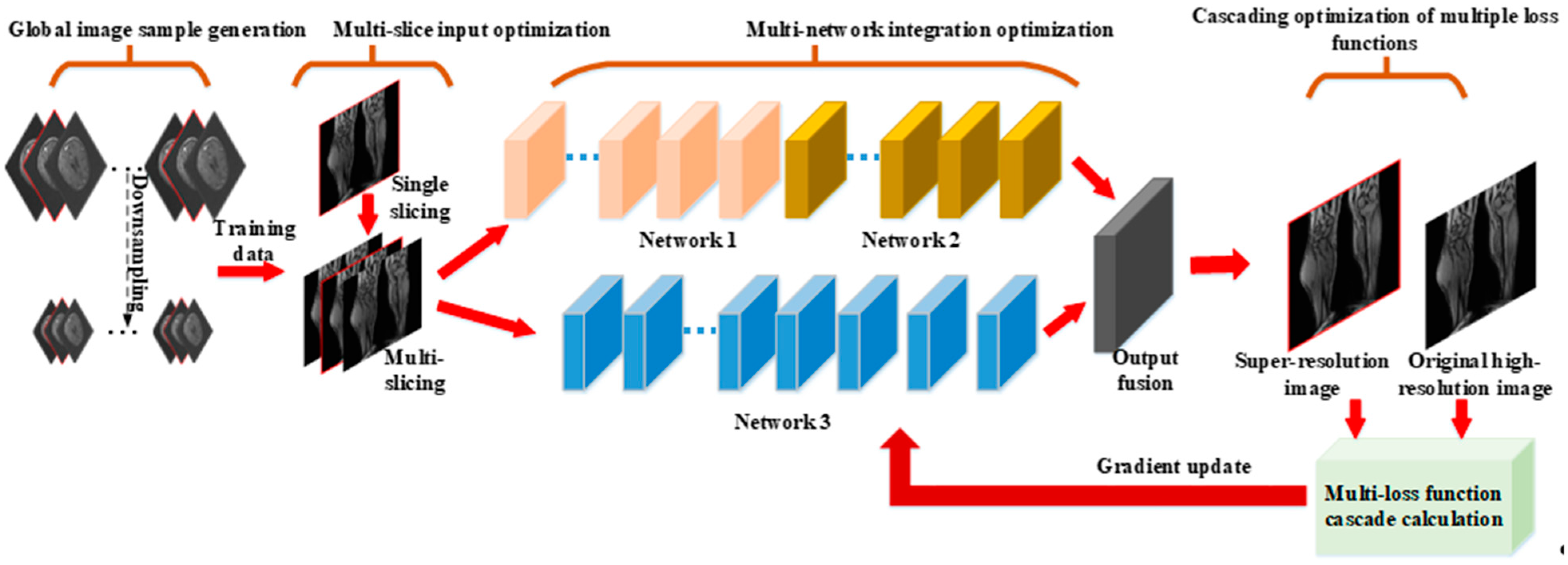
In order to solve the three limitations of deep super-resolution networks on MR images simultaneously, this paper proposes a multi-optimized ESRFBN super-resolution network algorithm for MR images based on the optimization methods of the previous three paragraphs. The algorithm architecture is shown in Figure 1. The three optimization methods are applied to the ESRFBN network at the same time, so that the multi-optimized ESRFBN network can get a better MR images’ super-resolution effect.

2.1. Cascade Optimization of Loss Function Based on Joint PSNR-SSIM

In order to improve the PSRN and SSIM indexes of MR super-resolution, a cascade optimization method based on the joint loss function of PSNR-SSIM is proposed in this section. SSIM as a loss function is not particularly sensitive to uniform deviation. This leads to changes in brightness or color, which usually become duller. However, SSIM can preserve contrast and is better than other loss functions in the high-frequency region. On the other hand, the L1 loss function can keep the brightness and color unchanged. Therefore, in order to obtain the best characteristics of the two loss functions, this section combines them to form a new loss function, and the name is Mix loss function. Its formula is as follows

$$L^{\mathrm{Mix}}=\alpha \cdot L^{\mathrm{MS}-\mathrm{SSIM}}+(1-\alpha )\cdot G_{{\sigma }_G^M}\cdot L^{{\ell }_1}$$

(1)

The cascade optimization calculation steps of the loss function based on joint PSNR-SSIM are as follows.

• Step 1. Calculate $L^{\mathrm{MS}-\mathrm{SSIM}}$

SSIM/MS-SSIM is an index that measures the similarity of two images, mainly from three aspects: brightness, contrast and structure. Therefore, the SSIM index can better characterize the structural information of the image. As a loss function, it can better retain the high-frequency information of the image, so that the super-resolution image has more detailed information, which is useful for MR images in clinical diagnosis. Its expression is as follows. Where $y$ is the original high-resolution image; $y^{\prime }$ is the high-resolution image output by the deep network; ${\mu }_y$ is the mean of the image $y$; ${\mu }_{y^{\prime }}$ is the mean of the image $y^{\prime }$; ${\sigma }_y^2$ is the variance of the image $y$; ${\sigma }_{y^{\prime }}^2$ is the variance of the image $y^{\prime }$; ${\sigma }_{y^{\prime }y }$ is the covariance of the sum of the image $y$ and $y^{\prime }$; $c_1$ and $c_2$ are two constants, avoiding the denominator to be 0.

$$SSIM(y,y^{\prime })=\frac{(2{\mu }_{y^{\prime }}{\mu }_y+c_1)({\sigma }_{y^{\prime }y}+c_2)}{({\mu }_{y^{\prime }}^2+{\mu }_y^2+c_1)({\sigma }_{y^{\prime }}^2+{\sigma }_y^2+c_2)}$$

(2)

The index range of SSIM is 0–1. The larger the SSIM is, the higher the similarity of the two images. Therefore, SSIM as the loss function can be expressed as the following formula [20].

$$L^{SSIM}=1-SSIM(y,y^{\prime })$$

(3)

In order to better transmit the error, the SSIM formula is deformed, and the dependence of the mean and standard deviation on the pixel $p$ is ignored here. The mean and standard deviation are calculated using a Gaussian filter with a standard deviation $G_{\sigma G}$.

$$SSIM(y,y^{\prime })=\frac{(2{\mu }_{y^{\prime }}{\mu }_y+c_1)({\sigma }_{y^{\prime }y}+c_2)}{({\mu }_{y^{\prime }}^2+{\mu }_y^2+c_1)({\sigma }_{y^{\prime }}^2+{\sigma }_y^2+c_2)}=l(p)·cs(p)$$

(4)

At the same time, the SSIM loss function can be re-characterized as

$$L^{SSIM}(P)=1-SSIM(\tilde{p})$$

(5)

$\tilde{p}$ represents the central pixel. Even if the network learns the weight to maximize the SSIM value of the central pixel, the learned kernel will be applied to all pixels in the image. Therefore, it is necessary to calculate the reciprocal of $\tilde{p}$ to other pixels $q$, and the derivation process is as follows

$$\frac{\partial L^{SSIM}(P)}{\partial x(q)}=-\frac{\partial }{\partial x(q)}SSIM(\tilde{p})=-(\frac{\partial l(\tilde{p})}{\partial x(q)}·cs(\tilde{p})+l(\tilde{p})·\frac{\partial cs(\tilde{p})}{\partial x(q)})$$

(6)

where

$$\frac{\partial l(\tilde{p})}{\partial x(q)}=2·G_{\sigma G}(q-\tilde{p})·(\frac{{\mu }_y-{\mu }_{y^{\prime }}l(\tilde{p})}{{\mu }_y^2+{\mu }_{y^{\prime }}^2+c_1})$$

(7)

$$\frac{\partial cs(\tilde{p})}{\partial x(q)}=\frac{2}{{\sigma }_y^2+{\sigma }_{y^{\prime }}^2+c_2}·G_{\sigma G}(q-\tilde{p})·[(y(q)-{\mu }_y)-cs(\tilde{p})·(y^{\prime }(q)-{\mu }_{y^{\prime }})]$$

(8)

$G_{\sigma G}(q-\tilde{p})$ is the Gaussian coefficient associated with pixel q.

For MS-SSIM, it can be expressed as follows, where $\alpha ={\beta }_j=1$

$$MS-SSIM(p)=l_M^{\alpha }(p)·{\displaystyle \prod _{j=1}^{M}c{s}_j^{{\beta }_j}(p)}$$

(9)

Analogous to SSIM as a loss function, MS-SSIM as a loss function can be characterized as

$$L^{MS-SSIM}(P)=1-MS-SSIM(\tilde{p})$$

(10)

• Step 2. Calculate $L^{l_1}$

Both the L1 and L2 loss function can keep the brightness and color unchanged, but the L2 loss function is more sensitive to abnormal points; thus, the effect of the model will be greatly affected the data quality.

The mechanism of the L1 loss function on the image is based on comparing the differences per pixel and then taking the absolute value. In general, it minimizes the sum of the absolute difference between the target value and the estimated value. The expression is shown below, where $y(i,j)$ represents the pixel value of the original high-resolution image at position $(i,j)$; $y^{\prime }(i,j)$ represents the pixel value of the network output image at position $(i,j)$; W and H represent the width and height of the image, respectively [20].

$$L^{l_1}=\frac{1}{WH}{\displaystyle \sum _{i=0}^M\sum _{j=0}^N|y(i,j)-y^{\prime }(i,j)|}$$

(11)

$$L^{l_2}=\frac{1}{WH}{\displaystyle \sum _{i=0}^M\sum _{j=0}^N({y(i,j)-y^{\prime }(i,j))}^2}$$

(12)

Compared with the L1 loss function, the L2 loss function magnifies the gap between the maximum error and the minimum error, and the L2 loss function is more sensitive to abnormal points. When the quality of the training data is poor, the L2 loss function will affect the model effect, resulting in inaccurate super-resolution effects, which will have a serious impact on medical diagnosis based on MR images. However, if only the L1 loss function is used, it is easy to fall into a local optimal solution.

• Step 3. Setting of α

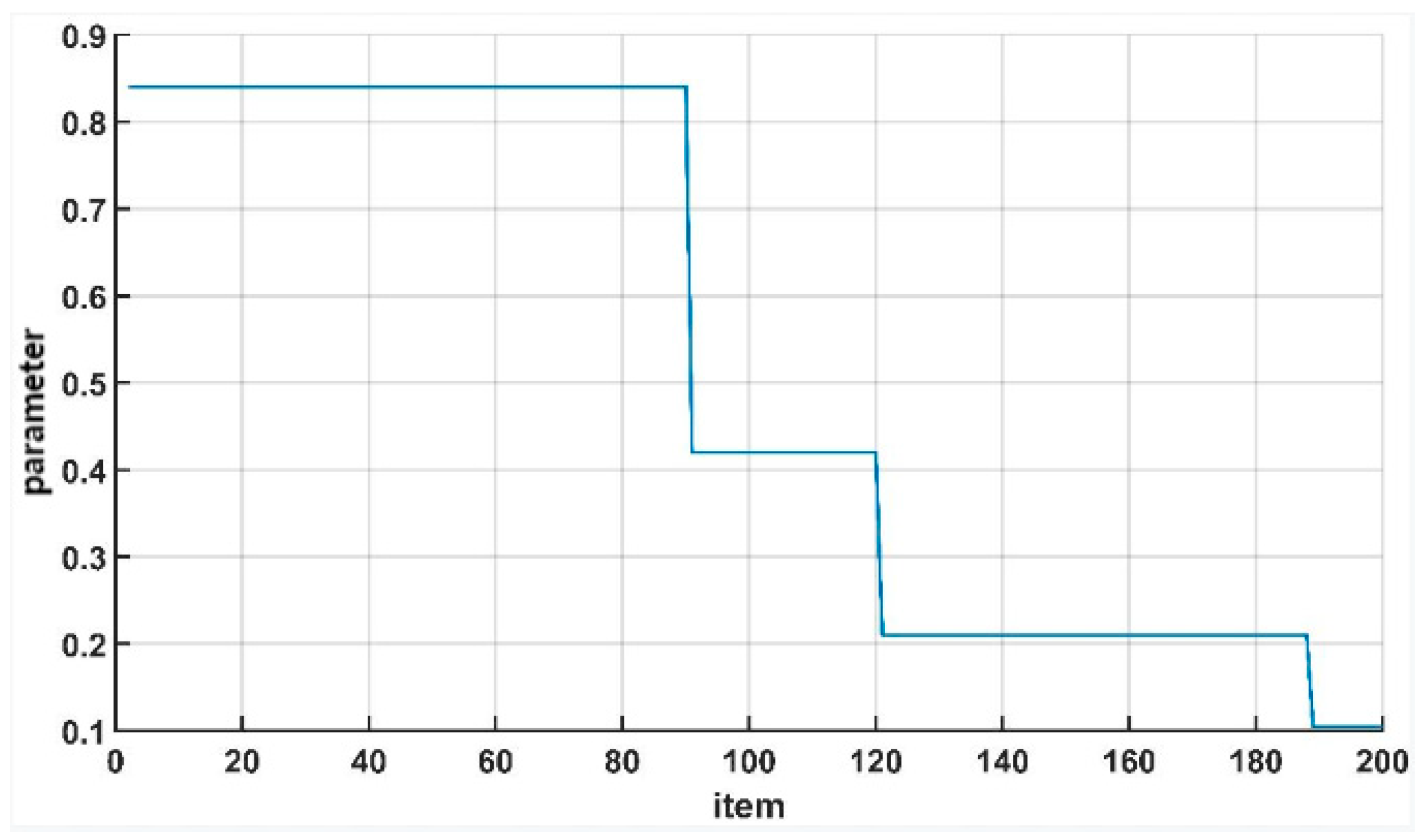
The initial value of α in the formula is set to 0.84. In this section, half attenuation was carried out in the 90th epoch, the 120th epoch and the 190th epoch, respectively, which can be conducive to the rapid convergence of the network.

2.2. ESRFBN Network Improvement Based on Contextual Network Fusion

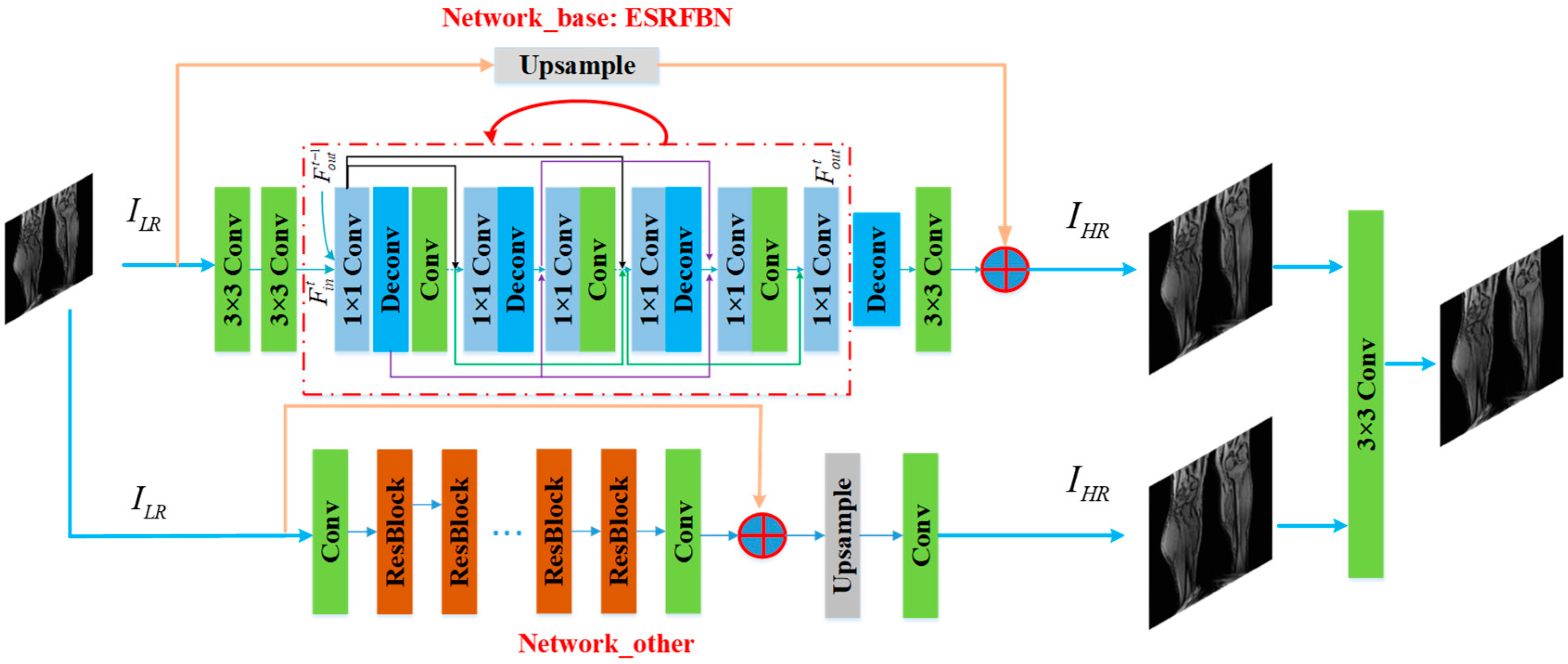
The ESRFBN network improvement based on contextual network fusion is shown in Figure 2. For the input low-resolution MR images, it is divided into two channels and two input network architectures, respectively. For the first channel, the images are computed with the calculation of 3 × 3 convolution, 1 × 1 convolution and deconvolution and the up-sampling operation. Through these computer units, the high-resolution image is created. In the second channel of images, a high-resolution image is obtained through the second network computing. Then, the high-resolution images are created with the convolution-based fusion network from the two channels of MR images from the super-resolution networks. Two independent networks are used to predict high-resolution images, respectively, and the fusion layer is used to fuse the high-resolution images outputted by the independent network, then output the final super-resolution image. The expression is as follows [20].

$${\stackrel{⌢}{y}}_i=F_{\{S_1,S_2,\cdots ,S_M\}}(x_i)=\sum _{j=1}^M{W}_j\ast S_j(x_i)+b_j$$

(13)

Among them, $W_j,b_j$ is the fusion layer parameter that being constructed. The weight of the fusion layer can be learned by fine-tuning the entire network. In this section, two independent network parameters are frozen to learn the parameters of the fusion layer. A 3 × 3 convolution layer is used as the fusion layer, and its learnable parameter is 3 × (3 × 3 + 1) = 30. In the training of the improved ESRFBN network method based on contextual network fusion, the weight of a single network is frozen, and the fusion layer is randomly initialized by a zero-mean Gaussian distribution with a standard deviation of 0.001.

2.3. Algorithm Flow

In this section, the steps of the ESRFBN super-resolution network algorithm for MR images based on multiple optimizations are mainly divided into network training and model testing. The specific steps are in the Appendix A.

2.4. Discussion

Firstly, under the large number of the training samples, the super-resolution performance is better if the super-resolution network is deeper. Accordingly, the number of the parameters of the deep super-resolution network is larger. Secondly, under the similar number of parameters and training samples, the different structures of the deep network have the different ability of super-resolution. The different performances depend on the different super-resolution mechanism. So, we have the fusion of the different structure of networks, and the fusion network can extract enough of the features of the MR images. Then, the higher super-resolution performance is obtained with the fusion super-resolution deep network. In this fusion network, we fuse the independent deep super-resolution networks, so the size of networks is not decreased. So, the numbers of parameters are similar for the original different super-resolution networks and fusion network. On the balance of the performance and the complexity, on the same size of the deep networks, the fusion network can achieve the higher performance than the original scale of deep network. For multiple independent deep super-resolution networks, the output of a single network is integrated through an additional fusion layer, which broadens the width of the network, and can effectively improve the mapping and characterization capabilities of high- and low-resolution features.

3. Experimental Results and Analysis

3.1. Experiment 1

In this section, the loss function experiments of L1, L2, SSIM, MS-SSIM and L1+MS-SSIM are performed on the double cubic down-sampling data set and K-space truncated data set. The specific experimental results are shown in

Table 1. PSNR values of different loss functions (bicubic downsampling).

Data	Scale	Bicubic	L1	L2	SSIM	MS-SSIM	L1+MS-SSIM
neck	×2	25.44	37.89	40.41	40.24	40.15	40.47
	×4	21.58	30.28	30.90	30.50	30.67	30.92
breast	×2	28.56	35.13	41.46	42.90	42.83	42.97
	×4	20.50	30.78	32.88	32.60	32.91	32.93
knee	×2	30.60	38.39	40.12	40.04	40.12	40.20
	×4	22.69	31.42	32.63	32.29	32.51	32.64
head	×2	20.32	39.42	38.55	38.19	38.28	39.39
	×4	18.60	34.04	32.97	32.20	31.95	34.11

Note: The numbers in bold are the best results.

,

Table 2. SSIM values of different loss functions (double cubic downsampling).

Data	Scale	Bicubic	L1	L2	SSIM	MS-SSIM	L1+MS-SSIM
neck	×2	0.6928	0.9876	0.9900	0.9900	0.9898	0.9897
	×4	0.5442	0.9308	0.9349	0.9367	0.9358	0.9392
breast	×2	0.8848	0.9492	0.9763	0.9802	0.9797	0.9816
	×4	0.4830	0.8979	0.9031	0.9070	0.9075	0.9082
knee	×2	0.9185	0.9760	0.9633	0.9641	0.9637	0.9774
	×4	0.5649	0.8987	0.8844	0.8881	0.8867	0.8873
head	×2	0.6025	0.9605	0.9592	0.9597	0.9593	0.9609
	×4	0.5623	0.9128	0.9064	0.9064	0.9011	0.9609

,

Table 3. PSNR values of different loss functions (K-space truncation downsampling).

Data	Scale	Bicubic	L1	L2	SSIM	MS-SSIM	L1+MS-SSIM
neck	×2	15.80	24.16	24.32	23.98	24.24	24.36
	×4	9.29	18.54	19.76	18.85	19.26	19.77
breast	×2	13.52	31.75	31.82	31.78	31.96	31.98
	×4	7.68	25.62	25.94	25.15	25.98	25.98
knee	×2	11.83	31.49	31.52	30.81	31.09	31.73
	×4	5.97	26.09	26.31	24.86	25.48	26.49
head	×2	6.29	27.89	29.87	26.98	27.97	28.76
	×4	2.95	20.75	20.43	20.97	18.53	20.98

Note: The numbers in bold are the best results.

and

Table 4. SSIM values of different loss functions (K-space truncation downsampling).

Data	Scale	Bicubic	L1	L2	SSIM	MS-SSIM	L1+MS-SSIM
neck	×2	0.6500	0.8923	0.8979	0.8997	0.8980	0.8998
	×4	0.3399	0.8201	0.8255	0.8292	0.8268	0.8315
breast	×2	0.4967	0.9123	0.9211	0.9206	0.9189	0.9213
	×4	0.0487	0.8027	0.8078	0.8111	0.8178	0.8185
knee	×2	0.3647	0.9008	0.9072	0.9073	0.9054	0.9078
	×4	0.0919	0.7840	0.7908	0.7858	0.7864	0.7864
head	×2	0.3126	0.8065	0.8211	0.8997	0.8075	0.9609
	×4	0.2081	0.6434	0.6336	0.6503	0.6508	0.6539

Note: The numbers in bold are the best results.

. When ESRFBN uses cascading loss function L1+MS-SSIM as a loss function for training, the effect is optimal on both the bicubic decrement sampling data set and K-space truncated data set, which indicates the effectiveness of the optimization of the cascading loss function.

SSIM, as a loss function, is not particularly sensitive to uniform deviations, which will cause changes in brightness or color, and usually become duller. However, SSIM can preserve contrast and is better than other loss functions in the high-frequency region. On the other hand, the L1 loss function can keep the brightness and color unchanged. Therefore, the cascaded loss function can combine the characteristics of the two well, so that the super-resolution effect of the trained network is better.

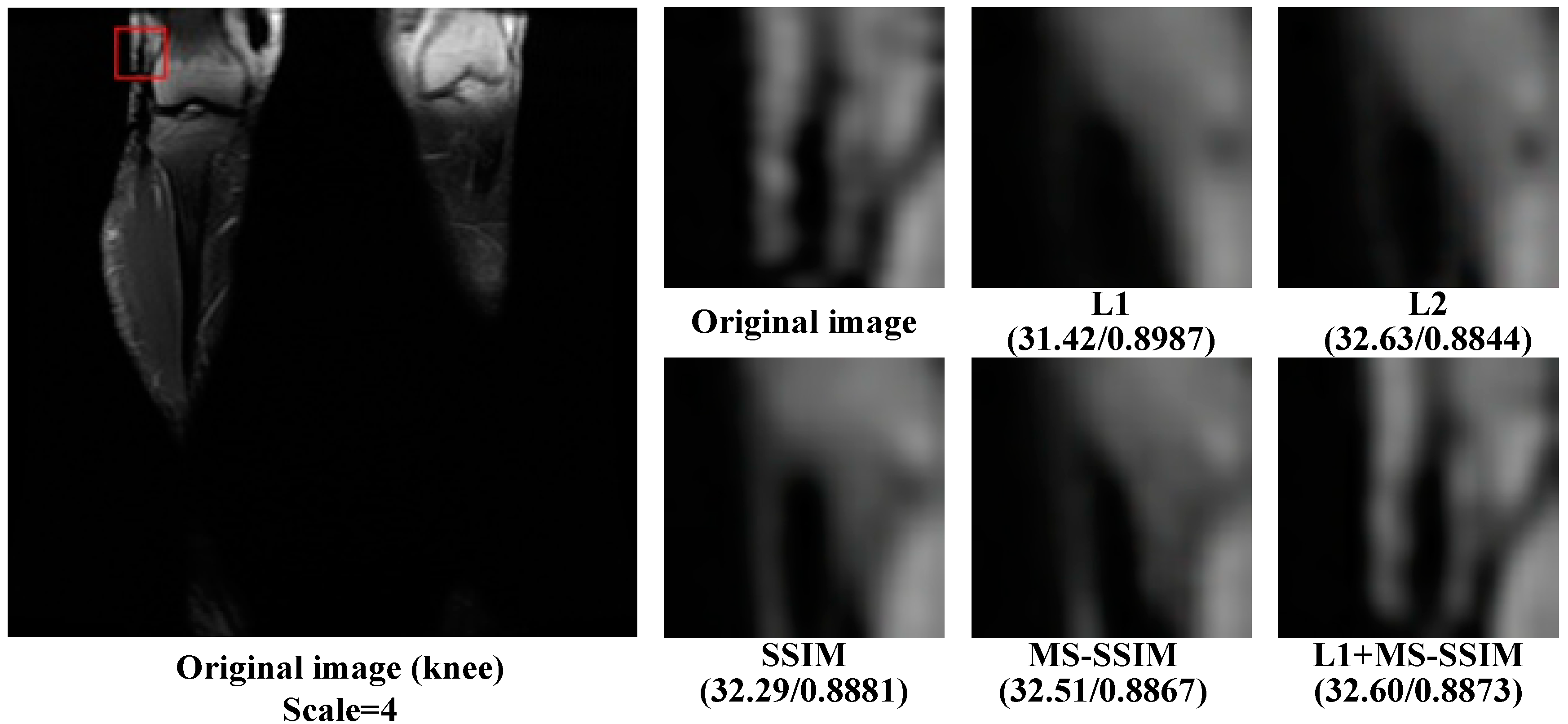
As can be seen from Figure 3, compared with SSIM and MS-SSIM loss functions, the result of L1 and L2 only improves the pixels around the contour details, while for the result of SSIM and MS-SSIM loss functions, the feature details of high-resolution images after super-resolution are more prominent than that of L1 and L2. However, the L1+MS-SSIM loss function retains both pixel gray level information and contour feature information, and the image after super-resolution is most similar to the original image. It also indicates that the ESRFBN super-resolution network based on the L1+MS-SSIM cascading loss function optimization can effectively improve the super-resolution effect of MR images.

3.2. Experiment 2: Analysis of the Convergence of Each Loss Function Index during the Training Process

In order to enable the network to converge better during the training process and avoid falling into the local optimal solution, the cascaded loss function L1+MS-SSIM uses parameter $\alpha$ to balance the PSNR index and the SSIM index. As can be seen from the training convergence curve of the ESRFBN network in Figure 4, it began to converge before 80 epochs. Uncertain factors in the calculation of loss function were increased by adjusting the attenuation of the learning rate and parameter $\alpha$, so as to avoid falling into the local optimal solution. The attenuation of parameter $\alpha$ is shown in Figure 4, which is attenuated by half at the 90th epoch, 120th epoch and 190th epoch, respectively.

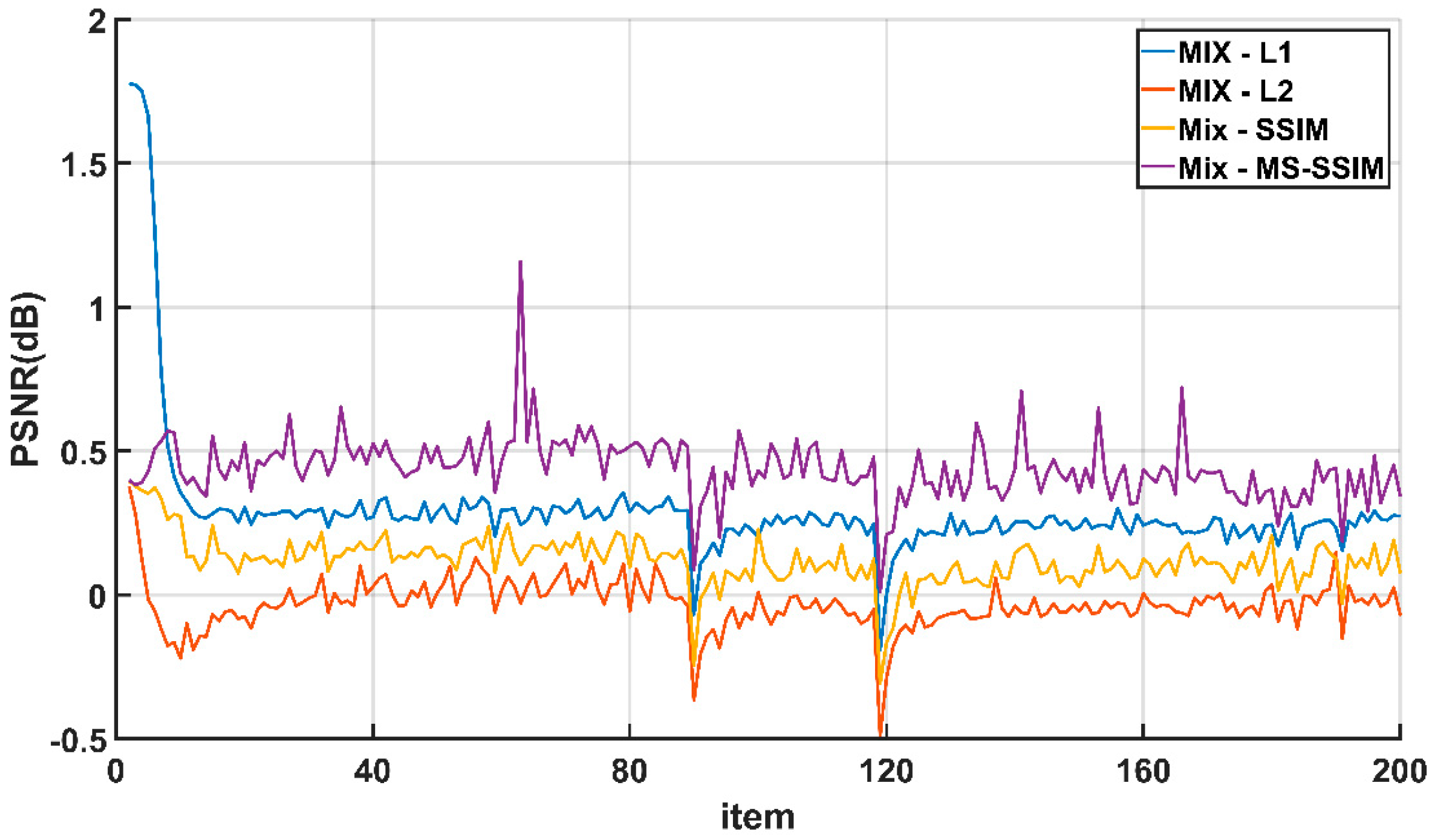
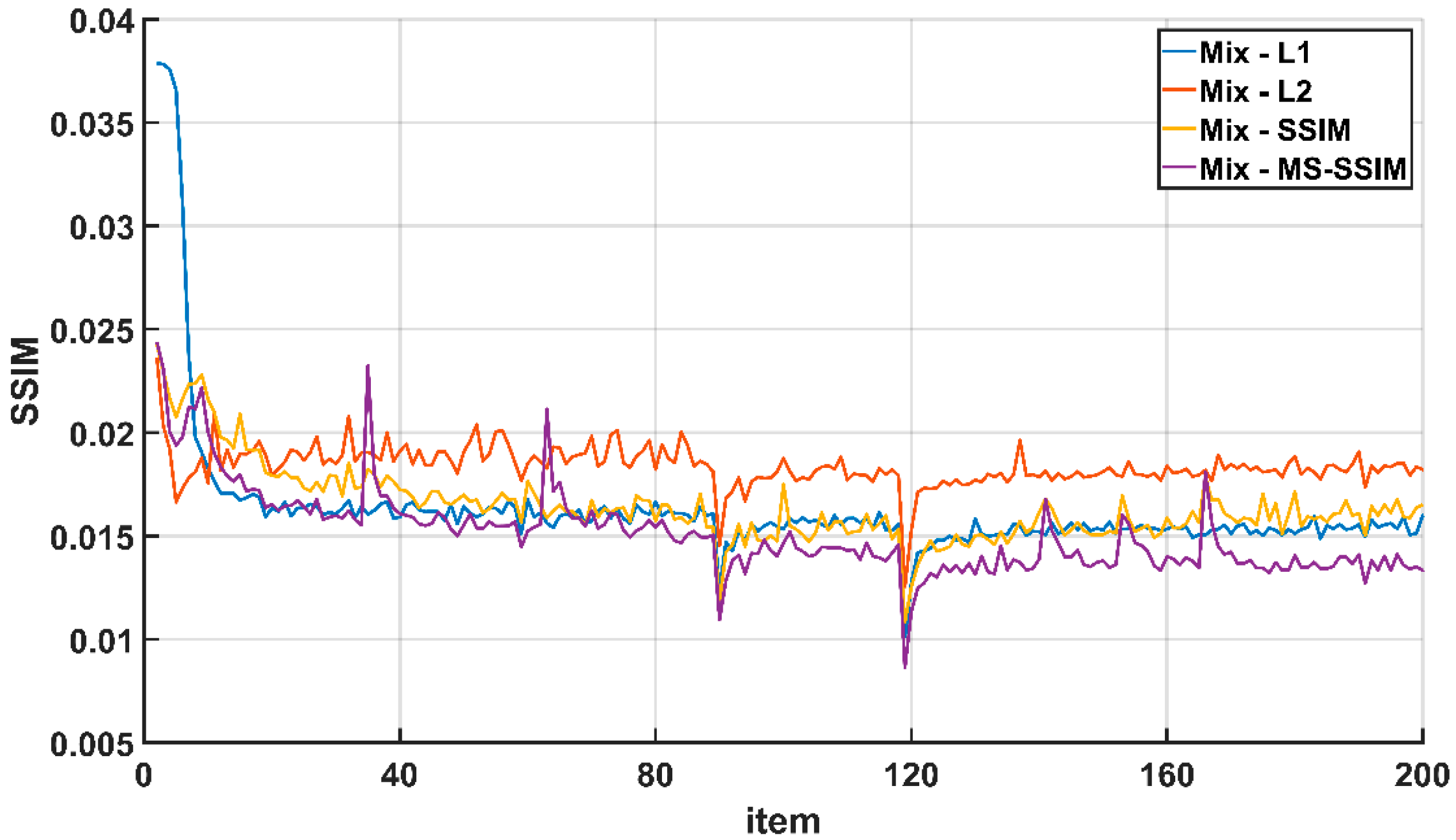
In this section, in order to reflect the impact of parameter $\alpha$’s attenuation on the training process better, the difference between the evaluation indexes of the cascaded loss function (Mix) and other loss functions during the training process is used for characterization. Figure 5 shows the curve of the number of iterations and the difference in PSNR during the training of each loss function, and Figure 6 shows the curve of the number of iterations and the difference in the SSIM during the training of each loss function. It can be seen from the figure that at 90 epoch and 120 epoch, the difference between the Mix loss function and other loss functions will have obvious vibrations. This is because in the Mix loss function, the parameter $\alpha$ attenuated and the loss function curve oscillates, resulting in lower PSNR and SSIM values calculated by the model. However, the difference tends to stabilize after rising in the subsequent process. This shows that ESRFBN has a strong convergence ability. On the other hand, it shows that during the training process, the learning rate attenuation strategy can prevent the network from falling into the local optimal solution, so that the network model obtained finally has a better super-resolution effect.

In order to improve the PSRN and SSIM indexes of MR super-resolution, this section proposes a method based on PSNR-SSIM joint loss function cascade optimization. In order to verify the effectiveness of the proposed method, four experiments were carried out on the data sets generated by the two modes.

Experiment 1 proves that the L1+MS_SSIM cascaded loss function can obtain the optimal super-resolution effect, which proves the effectiveness of the optimization of the cascading loss function. This is mainly because the cascading loss function combines the advantages of the L1 loss function which can keep the brightness and color unchanged and the MS_SSIM loss function which can retain the contrast and is better than other loss functions in the high frequency area, so that the cascading loss function has the best characteristics of the two loss functions. The cascade loss function optimization enables the ESRFBN network to obtain a better super-resolution effect of MR images.

Through Experiment 2, it can be proved that parameter attenuation can make the difference between the Mix loss function and other loss functions vibrate significantly, so as to avoid the network falling into the local optimal solution and make the obtained network model have better super-resolution effect. At the same time, it shows that the ESRFBN network has strong convergence ability, which can make deep network converge quickly in the training process and reduce the learning difficulty of network.

The data set used in this section includes MR images’ data of the neck, head, breast and knee. The number of training set, verification set and test set are: Neck: 400, 50, 50; Head: 500, 50, 50; breast: 1800, 200, 200; knee: 800, 100, 100. Data sets with two super-resolution scales of ×2 and ×4 are generated. The model used is implemented with Pytorch 1.6.0, and is trained with dual Nvidia GeForce GTX 1080 Ti graphics cards.

3.3. Performance Evaluation

In this section, the proposed multi-optimization ESRFBN super-resolution network algorithm for MR images is compared with the super-resolution algorithm based on interpolation, reconstruction, dictionary learning and deep learning. The algorithms include BIC [15], IBP [16], POCS [5], MAP [6], JDL [7], IJDL [17], RDN [11], EDSR [18], SRGAN [12], ESRGAN [19], SRFBN [14], ESRFBN [20].

The methods mentioned in this section and the experimental results of each method are shown in

Table 5. PSNR values of MR images ESRFBN super-resolution network based on multiple optimization.

Data	Scale	BIC	IBP	POCS	MAP	JDL	IJDL	RDN	EDSR	DBPN	SRGAN	ESRGAN	SRFBN	ESRFBN	Proposed
neck	×2	25.44	29.35	28.86	30.01	35.95	36.12	29.05	37.34	35.74	37.69	36.16	38.03	37.89	42.96
	×4	21.58	24.72	24.28	25.27	28.53	28.82	24.53	29.25	29.28	28.78	29.11	30.23	30.28	36.22
breast	×2	28.56	30.06	29.76	31.21	33.34	34.08	33.50	34.57	31.94	34.06	32.91	34.28	35.13	41.03
	×4	20.50	21.56	22.38	23.09	27.87	29.16	23.68	30.00	28.13	27.99	26.31	30.68	30.78	36.85
knee	×2	30.60	32.80	33.01	34.36	35.94	36.87	36.34	37.49	37.67	36.93	36.00	37.95	38.39	43.81
	×4	22.69	24.74	25.25	26.66	28.48	30.11	30.02	28.34	31.29	29.63	28.75	31.35	31.42	37.07
head	×2	20.32	28.22	28.04	31.24	33.43	35.11	38.05	38.03	33.82	35.80	35.89	39.19	39.42	42.86
	×4	18.60	20.35	22.29	24.68	28.65	28.60	29.70	32.22	29.39	30.95	31.32	33.60	34.04	38.72

Note: The numbers in bold are the best results.

and

Table 6. SSIM values of MR images ESRFBN super-resolution network based on multiple optimization.

Data	Scale	BIC	IBP	POCS	MAP	JDL	IJDL	RDN	EDSR	DBPN	SRGAN	ESRGAN	SRFBN	ESRFBN	Proposed
neck	×2	0.6928	0.8024	0.8257	0.8458	0.9155	0.9386	0.8824	0.9861	0.9800	0.9868	0.9821	0.9879	0.9880	0.9899
	×4	0.5442	0.7589	0.8016	0.8274	0.9001	0.9318	0.7144	0.9164	0.9182	0.9093	0.9158	0.9304	0.9308	0.9524
breast	×2	0.8848	0.8943	0.9010	0.9046	0.9200	0.9308	0.9373	0.9447	0.9243	0.9332	0.9256	0.9428	0.9492	0.9683
	×4	0.4830	0.7592	0.7759	0.7900	0.8594	0.8747	0.6118	0.8631	0.8351	0.8137	0.7900	0.8735	0.8979	0.9401
knee	×2	0.9185	0.9231	0.9210	0.9342	0.9591	0.9660	0.9641	0.9719	0.9727	0.9670	0.9634	0.9744	0.9760	0.9865
	×4	0.5649	0.6491	0.6507	0.6875	0.8476	0.8522	0.8597	0.8968	0.8940	0.8643	0.9077	0.8964	0.9054	0.9641
head	×2	0.6025	0.8522	0.8483	0.8427	0.9018	0.9274	0.9565	0.9565	0.9062	0.9234	0.9241	0.9600	0.9605	0.9811
	×4	0.5623	0.7295	0.7535	0.7624	0.8358	0.8601	0.7962	0.8886	0.7906	0.8500	0.8611	0.9089	0.9128	0.9546

Note: The numbers in bold are the best results.

. It can be seen from the table that the method proposed in this paper has obtained the best results in four parts of the human body and in two super-division scales, and the evaluation index value improved greatly. Compared with the suboptimal method under the scale ×2, the PSNR value is increased by 4.93, 5.90, 5.42 and 3.44, respectively; the SSIM value is increased by 0.0019, 0.0191, 0.0105 and 0.0206, respectively. Under the scale ×4, the PSNR values were increased by 5.94, 6.07, 5.65 and 4.68; the SSIM values were increased by 0.0216, 0.0422, 0.0564 and 0.0418. From the improvement of the index value, it can be seen that the MR image ESRFBN super-resolution network based on multiple optimizations proposed in this section is more suitable for MR image super-resolution tasks, and can effectively solve the limitations of deep learning networks in the application of MR images’ super-resolution tasks. The experimental results prove the effectiveness of the method proposed in this section.

4. Conclusions

This paper aims at solving the three limitations of applying a deep learning network in the super-resolution task of MR images, such as not fully considering the characteristics of MR images’ sequence, difficulty in obtaining the optimal solution of loss function and difficulty in balancing model complexity and training difficulty. Firstly, seven kinds of deep learning networks with a good super-resolution effect were used to carry out experiments under two super-resolution scales on four human body parts, namely neck, breast, knee and head. Secondly, in view of the three limitations of applying deep learning in the super-resolution of MR images, this paper proposes a multiple optimization-based ESRFBN super-resolution network algorithm for MR images, which integrates the three optimization methods. The quantitative experimental results show that the ESRFBN network is more suitable for MR images’ super-resolution task. Secondly, in view of the three limitations of applying deep learning in the super-resolution of MR images, this paper proposes a multiple optimization-based ESRFBN super-resolution network algorithm for MR images, which integrates the three optimization methods. Quantitative experimental results show that the ESRFBN super-resolution network based on multiple optimization of MR images is superior to the super-resolution algorithms based on interpolation, reconstruction, dictionary learning and other super-resolution algorithms based on a deep learning network, and it can greatly improve the super-resolution effect of MR images, proving that the method proposed in this paper is effective.

References

- El Hakimi, W.; Wesarg, S. Accurate super-resolution reconstruction for CT and MR images. In Proceedings of the 26th IEEE International Symposium on Computer-Based Medical Systems, Porto, Portugal, 20–22 June 2013; pp. 445–448. [Google Scholar]
- Zhao, C.; Lu, J.; Li, K.; Wang, X.; Wang, H.; Zhang, M. Optimization of scanning time for clinical application of resting fMRI. Chin. J. Mod. Neurol. Dis. 2011, 3, 51–55. [Google Scholar]
- Kaur, P.; Sao, A.K.; Ahuja, C.K. Super Resolution of Magnetic Resonance Images. J. Imaging 2021, 7, 101. [Google Scholar] [CrossRef]
- Ramasubramanian, V.; Paliwal, K.K. An efficient approximation-elimination algorithm for fast nearest-neighbour search based on a spherical distance coordinate formulation. Pattern Recognit. Lett. 1992, 13, 471–480. [Google Scholar] [CrossRef]
- Stark, H.; Oskoui, P. High-resolution image recovery from image-plane arrays, using convex projections. J. Opt. Soc. Am. A Opt. Image Sci. 1989, 6, 1715. [Google Scholar] [CrossRef] [PubMed]
- Schultz, R.R.; Stevenson, R.L. Improved definition image expansion. In Proceedings of the IEEE International Conference on Acoustics, San Francisco, CA, USA, 23–26 March 1992. [Google Scholar]
- Yang, J.; Wright, J.; Huang, T.S.; Ma, Y. Image Super-Resolution Via Sparse Representation. IEEE Trans. Image Process. 2010, 19, 2861–2873. [Google Scholar] [CrossRef] [PubMed]
- Dong, C.; Loy, C.C.; He, K.; Tang, X. Image Super-Resolution Using Deep Convolutional Networks. IEEE Trans. Pattern Anal. Mach. Intell. 2016, 38, 295–307. [Google Scholar] [CrossRef] [PubMed] [Green Version]
- Wang, Z.; Chen, J.; Hoi, S. Deep Learning for Image Super-resolution: A Survey. IEEE Trans. Pattern Anal. Mach. Intell. 2020, 99, 1. [Google Scholar] [CrossRef] [PubMed] [Green Version]
- Kim, J.; Lee, J.K.; Lee, K.M. Accurate Image Super-Resolution Using Very Deep Convolutional Networks. In Proceedings of the IEEE Conference on Computer Vision & Pattern Recognition, Las Vegas, NV, USA, 27–30 June 2016; pp. 1646–1654. [Google Scholar]
- Zhang, Y.; Tian, Y.; Kong, Y.; Zhong, B.; Fu, Y. Residual Dense Network for Image Super-Resolution. In Proceedings of the 2018 IEEE/CVF Conference on Computer Vision and Pattern Recognition, Salt Lake City, UT, USA, 18–23 June 2018; pp. 2472–2481. [Google Scholar]
- Ledig, C.; Theis, L.; Huszar, F.; Caballero, J.; Cunningham, A.; Acosta, A.; Aitken, A.; Tejani, A.; Totz, J.; Wang, Z.; et al. Photo-Realistic Single Image Super-Resolution Using a Generative Adversarial Network. In Proceedings of the 2017 IEEE Conference on Computer Vision and Pattern Recognition (CVPR), Honolulu, HI, USA, 21–26 July 2017; pp. 5892–5900. [Google Scholar]
- Haris, M.; Shakhnarovich, G.; Ukita, N. Deep Back-Projection Networks for Super-Resolution. In Proceedings of the IEEE Conference on Computer Vision and Pattern Recognition (CVPR), Salt Lake City, UT, USA, 18–22 June 2018. [Google Scholar]
- Li, Z.; Yang, J.; Liu, Z.; Yang, X.; Jeon, G.; Wu, W. Feedback Network for Image Super-Resolution. In Proceedings of the IEEE/CVF Conference on Computer Vision and Pattern Recognition (CVPR), Long Beach, CA, USA, 16–20 June 2019. [Google Scholar]
- Keys, R. Cubic convolution interpolation for digital image processing. IEEE Trans. Acoust. Speech Signal Process. 1981, 29, 1153–1160. [Google Scholar] [CrossRef] [Green Version]
- Irani, M.; Peleg, S. Improving resolution by image registration. CVGIP Graph. Model. Image Process. 1991, 53, 231–239. [Google Scholar] [CrossRef]
- Li, J.B.; Liu, H.; Pan, J.S.; Yao, H. Training samples-optimizing based dictionary learning algorithm for MR sparse superresolution reconstruction. Biomed. Signal Process. Control 2018, 39, 177–184. [Google Scholar] [CrossRef]
- Lim, B.; Son, S.; Kim, H.; Nah, S.; Lee, K.M. Enhanced Deep Residual Networks for Single Image Super-Resolution. In Proceedings of the 2017 IEEE Conference on Computer Vision and Pattern Recognition Workshops (CVPRW), Honolulu, HI, USA, 21–26 July 2017. [Google Scholar]
- Wang, X.; Yu, K.; Wu, S.; Gu, J.; Liu, Y.; Dong, C.; Qiao, Y.; Loy, C.C. ESRGAN: Enhanced Super-Resolution Generative Adversarial Networks. In Proceedings of the European Conference on Computer Vision (ECCV) Workshops, Munich, Germany, 8–14 September 2018. [Google Scholar]
- Liu, H.; Liu, J.; Li, J.; Pan, J.S.; Yu, X. PSR: Unified Framework of Parameter-Learning-Based MR Image Superresolution. J. Healthc. Eng. 2021, 2021, 5591660. [Google Scholar] [PubMed]
- Xue, X.; Wang, Y.; Li, J.; Jiao, Z.; Ren, Z.; Gao, X. Progressive Sub-Band Residual-Learning Network for MR Image Super Resolution. IEEE J. Biomed. Health Inform. 2019, 24, 377–386. [Google Scholar] [CrossRef] [PubMed]
- Zheng, Y.; Zhen, B.; Chen, A.; Qi, F.; Hao, X.; Qiu, B. A hybrid convolutional neural network for super-resolution reconstruction of MR images. Med. Phys. 2020, 47, 3013–3022. [Google Scholar] [CrossRef] [PubMed]
- Tan, C.; Zhu, J. Arbitrary Scale Super-Resolution for Brain MRI Images. In Proceedings of the IFIP International Conference on Artificial Intelligence Applications and Innovations, Neos Marmaras, Greece, 5–7 June 2020. [Google Scholar]
- Hu, X.; Mu, H.; Zhang, X.; Wang, Z.; Tan, T.; Sun, J. Meta-SR: A magnification-arbitrary network for super-resolution. In Proceedings of the IEEE/CVF Conference on Computer Vision and Pattern Recognition, Long Beach, CA, USA, 16–20 June 2019; pp. 1575–1584. [Google Scholar]
- Xu, J.; Gong, E.; Pauly, J.; Zaharchuk, G. 200x Low-dose PET Reconstruction using Deep Learning. arXiv 2017, arXiv:1712.04119. [Google Scholar]
- Zhao, H.; Gallo, O.; Frosio, I.; Kautz, J. Loss Functions for Image Restoration with Neural Networks. IEEE Trans. Comput. Imaging 2016, 3, 47–57. [Google Scholar] [CrossRef]
- Ren, H.; El-Khamy, M.; Lee, J. Image Super Resolution Based on Fusing Multiple Convolution Neural Networks. In Proceedings of the Computer Vision & Pattern Recognition Workshops, Honolulu, HI, USA, 21–26 July 2017. [Google Scholar]
Figure 1.
The architecture of deep super-resolution algorithm based on multiple optimizations.
Figure 2.
The improved ESRFBN network method based on contextual network fusion.
Figure 3.
Knee: the super-resolution graph of each loss function of the ESRFBN network at scale 4.
Figure 4.
Attenuation of parameter .
Figure 5.
The scale of the knee part is 4: The PSNR difference between the training process of the Mix loss function and other loss functions.
Figure 6.
The scale of the knee is 4: The difference between the training process of the Mix loss function and other loss functions SSIM.