
Combining Signal Features of Ground-Penetrating Radar to Classify Moisture Damage in Layered Building Floors


1
Bundesanstalt für Materialforschung und-Prüfung (BAM), 12205 Berlin, Germany
2
Ingenieurbüro Tobias Ritzer GmbH, Lindenbachstrasse 29, 91126 Schwabach, Germany
3
Technische Universität Berlin, 10623 Berlin, Germany
*
Author to whom correspondence should be addressed.
Appl. Sci. 2021, 11(19), 8820; https://doi.org/10.3390/app11198820
Submission received: 29 July 2021
/
Revised: 14 September 2021
/
Accepted: 15 September 2021
/
Published: 23 September 2021
(This article belongs to the Special Issue Non-destructive Testing in Civil Engineering)
Abstract
:To date, the destructive extraction and analysis of drilling cores is the main possibility to obtain depth information about damaging water ingress in building floors. The time- and cost-intensive procedure constitutes an additional burden for building insurances that already list piped water damage as their largest item. With its high sensitivity for water, a ground-penetrating radar (GPR) could provide important support to approach this problem in a non-destructive way. In this research, we study the influence of moisture damage on GPR signals at different floor constructions. For this purpose, a modular specimen with interchangeable layers is developed to vary the screed and insulation material, as well as the respective layer thickness. The obtained data set is then used to investigate suitable signal features to classify three scenarios: dry, damaged insulation, and damaged screed. It was found that analyzing statistical distributions of A-scan features inside one B-scan allows for accurate classification on unknown floor constructions. Combining the features with multivariate data analysis and machine learning was the key to achieve satisfying results. The developed method provides a basis for upcoming validations on real damage cases.
1. Introduction
More than half of the building insurance claims in Germany (53%) are caused by piped water damage, which entailed costs of over 3 billion Euro in 2019 alone [1]. One reason for this, apart from generally ageing pipe systems, is that water leakage often remains unrecognized until signs of degradation become noticeable. At that point the extent of damage is already critical, which underlines the demand of an accurate determination and localization of water ingress.
Neutron probes [2] are already successfully applied on building floors to localize the source of damage and to identify affected areas. The radiated fast neutrons lose most of their kinetic energy when colliding with low-mass atoms. This is especially true for hydrogen. As a result, the fast neutrons are transformed into slow (thermal) neutrons, which are then detected by a counter tube inside the probe. Given that, the method is highly sensitive to moisture, however it cannot distinguish between chemically bound or fluid water. Therefore, a calibration must be done by the destructive extraction of drilling cores. These cores are also the only possibility to obtain additional information about the depth of moisture penetration. This is a time- and cost-intensive procedure, especially for building floors, where knowledge about the affected layer is essential to plan and perform efficient renovations. Here, ground-penetrating radar (GPR) can serve as a suitable addition to the neutron probe in order to classify common moisture damages in layered building floors in a non-destructive way.
The sensitivity of GPR for water has already been proven in many publications, especially in geophysics [3,4]. However, in civil engineering (CE), GPR is also increasingly being applied for non-destructive moisture measurements on building materials like asphalt, concrete, and screed [5,6,7,8,9,10]. Here, various methods have already been established. However, their adequate use and suitability highly depends on the particular case. Due to numerous possible uncertainties, like the given structure, installed materials, and layer thicknesses, interpreting GPR results is not straightforward and requires the expertise of trained personnel. These uncertainties often influence the same signal features that are used for moisture measurements (see Section 1.1). Here, relying on only one feature, as it is done in most of the related publications [11], can lead to high uncertainty.
In contrast, this work pursues the strategy of combining different features, which allows the use of multivariate data analysis. It aims to achieve an automated classification of three scenarios: (1) the dry state, (2) damaged insulation, and (3) a damaged screed, all of them on unknown floor constructions. This is accomplished by a machine learning approach trained with novel radargram features that consider the spatial continuity of the present damage. The features are extracted from an experimentally measured data set, including varying materials and layer thicknesses. Before discussing the methodology in Section 2, a short introduction to moisture measurements with GPR is given.
1.1. Moisture Measurement with GPR
Besides the mostly negligible conductivity and magnetic permeability, the electric permittivity is the governing material parameter for moisture measurements with GPR [12,13]. This gets particularly clear by comparing for dry concrete and water. Whereas the former lies between 2 to 9 [14], the latter shows values around 81. This difference causes a significant rise for wet concrete (between 10 to 20), which influences various propagation characteristics of the electromagnetic (EM) waves. By analyzing specific time-, amplitude-, or frequency-based features of the received signals, these water-related influences become measurable. A detailed review of those features typically used for moisture measurement with GPR in CE is presented in [11]. However, a short overview is given in the following. First, the velocity v of an EM wave is directly related to . For non-magnetic conditions, as it is usually the case in building materials, it can simply be calculated as follows [14,15]:
where c is the velocity of EM waves in free space, and T the two-way travel time in a material with the thickness D. Comparing the dry state of a material, sent and reflected pulses are received later for rising moisture content. Furthermore, the intensities and thus the measured amplitudes are reduced due to higher attenuations, caused by generally increased conductivity and more frequently occurring scattering events on water-filled pores. Filled pores also lead to Rayleigh scattering [16], which is one way to explain the observable shift of the received signals to lower frequencies for higher moisture content. Another explanation is given with the presence of dielectric dispersion, presented in the popular models of Debye [17] and Cole–Cole [18]. It describes the rising imaginary part of and the resulting absorption of higher-frequency components close to the relaxation frequency, which is 10 GHz to 20 GHz for free water [15,19], but can be smaller for porous materials. Another important characteristic of EM waves is the occurrence of reflection and transmission on material boundaries with different permittivities. With and of two mediums, an EM wave travelling from medium 1 to medium 2 is reflected by the amount of the reflection coefficient , which is calculated as follows [20]:
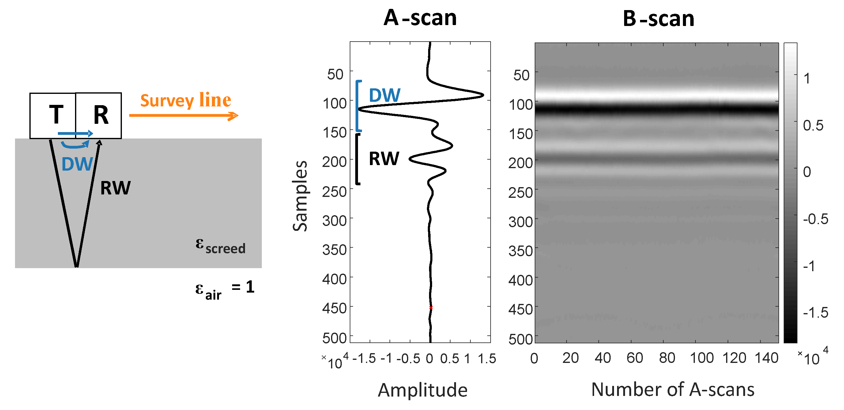
Therefore, the amplitude of a reflection wave (RW) is highly influenced by the boundary’s permittivity contrast, from which it originates. Figure 1 shows this simplified ray-based principle with an exemplary screed plate above air, forming such a permittivity contrast. It also presents the usually performed collection of multiple reflection signals (A-scans) along a survey line, whereas the offset between the transmitter (T) and receiver (R) stays constant (common-offset configuration). The recorded A-scans can then be combined in a radargram (B-scan) that offers the opportunity to visualize spatial deviations caused by inhomogeneities, like the presence of reinforcements or water-damaged areas.
The most dominant wave-type in an A-scan is the direct wave (DW), which travels the shortest path between T and R and is therefore recorded first. As shown, it is a superposition of an air and a ground wave and is generally used as a time reference for the following RW, since the moment of emitting the pulse (time zero) is unknown [21].
Typical signals and their respective features measured on layered floor constructions are discussed in Section 2.5.
2. Materials and Methods
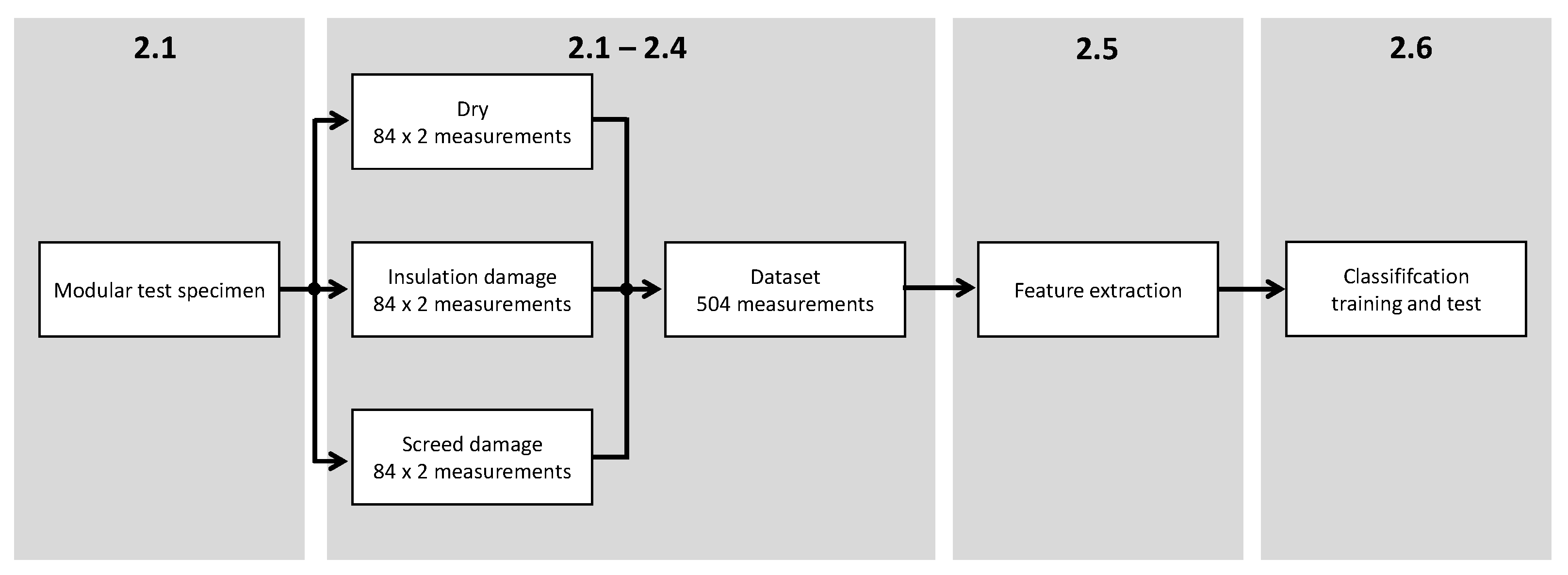
Figure 2 shows the general procedure of the work presented in this section. After introducing the designed modular test specimen in Section 2.1, the conducted experiments to obtain a dataset of three damage scenarios are discussed in the Section 2.1, Section 2.2, Section 2.3 and Section 2.4. In Section 2.5, various features are extracted to train and test different classifiers, which are shown in Section 2.6.
2.1. Modular Test Specimen
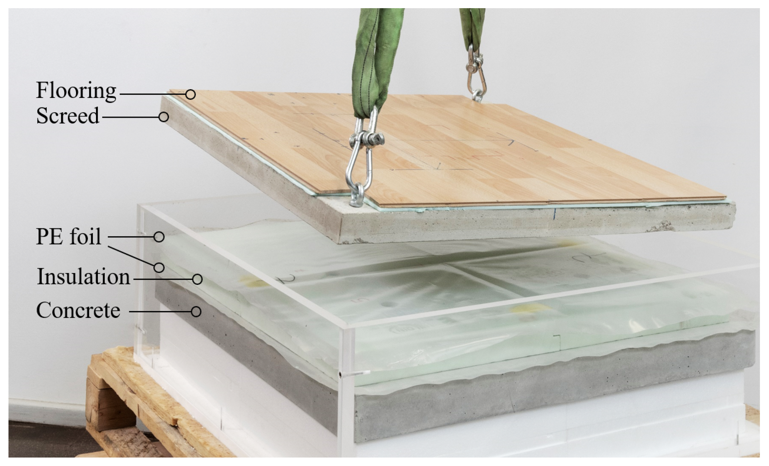
To study multiple different floor constructions, we designed a modular specimen (Figure 3), in which the screed and insulation layer can be exchanged in various ways according to the requirements of the experiment. The inner dimensions of 84 cm length, 84 cm width, and 30 cm height ensure sufficient space for the individual square-shaped parts with an edge length of 80 cm. Table 1 shows the variations of the chosen materials and their thicknesses that are believed to cover most floor setups in practice. Polyethylene (PE) foil is used to create a moisture barrier above and below the insulation. The influence of the laminate flooring and the concrete base layer on the presented classification method is considered to be negligible compared to the screed and insulation layer. Therefore, and with regard to the experimental effort, the flooring and base layer remained unchanged for the entire test series.
The cement and anhydrite screed were both chosen with the popular compressive strength C25 and the consistency class F5. The production process was carried out as instructed by the manufacturer. To guarantee efficient handling of the 60 kg to 100 kg heavy specimens, threaded sleeves were embedded in each corner. This allowed the temporary use of ring bolts to lift the plates.
The amount of different materials and thicknesses (Table 1) allows for the simulation of 84 different floor constructions for each of the three scenarios (252 setups in total). The experimental implementation of water damage in the insulation and screed layer is described in the following sections.
2.2. Water Damage in Insulation Layer
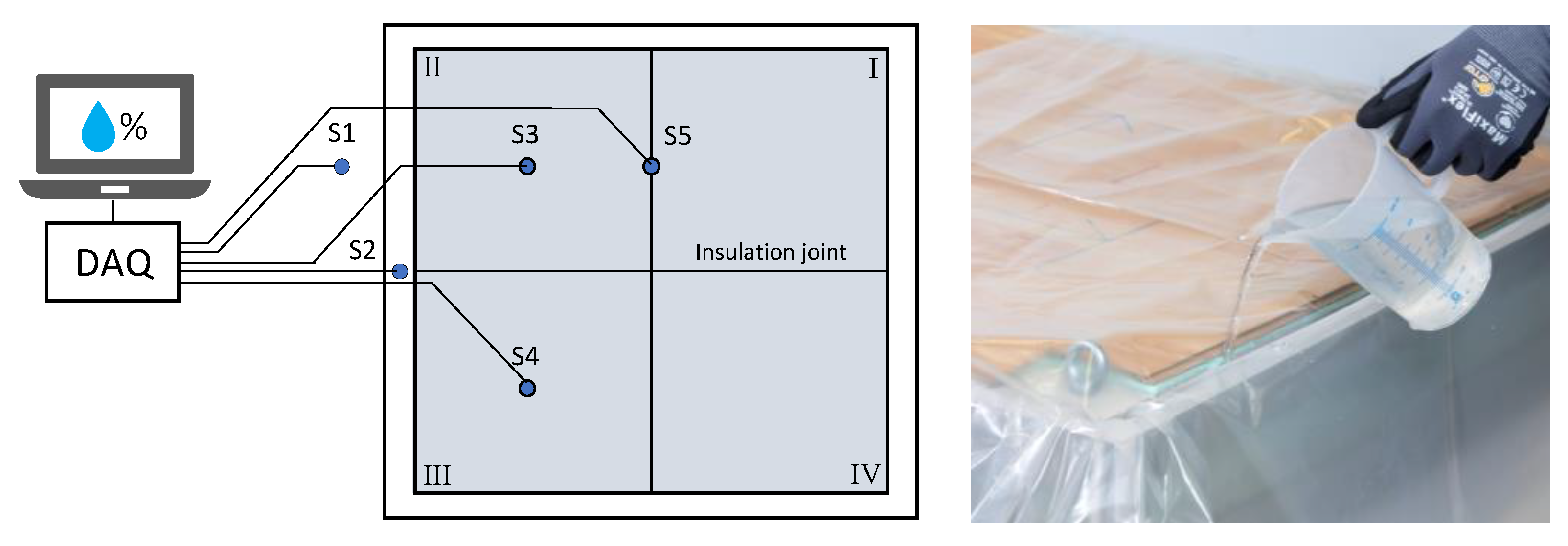
To evaluate the resulting damage of added water, HIH-5030 humidity sensors were embedded in the insulation material, as shown in Figure 4. For EP, XP, and GW, this was accomplished with drilling holes of 3 cm diameter and depths varying from 50% to 75% of the respective insulation thickness. Top sealing was attained with waterproof tape. For the fine-grained PS, drilling holes were not necessary because the sensors could be placed easily.
After adding equal amounts of water in all four sides of the setup, the moisture could spread for at least 12 hours to ensure stable conditions. In practical investigations, a threshold of 80% relative humidity is often considered as an adequate reason for renovations, since it provides optimum growth conditions for mould [22]. Following that, a setup was labeled as “damaged” only if all three sensors S3 to S5 exceeded this critical value. Thereafter, the measurement procedure, which is discussed in Section 2.4, was conducted for each of the six screeds.
2.3. Water Damage in Screed Layer
The quantification of screed moisture was carried out using the direct Darr method [23], which captures the loss of water by weighing samples before and after an oven-drying procedure. With the wet sample weight and the dry sample weight , the dry basis moisture content is calculated as follows:
Moisture content above 4 weight percent (wt%) and 0.5 wt% were valued as damage for cement and anhydrite screed, respectively. Due to preliminary investigations of the screed’s hydration process, was already known for each sample. Consequently, the sample’s moisture content could be obtained by measuring only. With 1.7 wt% to 2.3 wt% for CT and around 0.1 wt% for CA, these were rather low before simulating the damage. Therefore, we first flooded each sample by submersing them in water for 30 min (CT) or 10 min (CA). The moisture could then spread and evaporate for at least 2 days before the actual damage was induced. In consideration of practical screed damage that usually occurs after flooding from above, we then constantly poured water on top of the plates for 10 min. Besides continually weighing the samples, additional nuclear magnetic resonance (NMR) measurements were performed with the MOUSE [24,25] to obtain depth-resolved moisture distribution during the described saturation process. Figure 5 presents the exemplary NMR results with their respective water content measured on the 5 cm thick CT and CA screed.
Compared to CA, the CT screed shows an unbalanced water ingress for the sample’s top and bottom side after the submersion. We explain this with a lower porosity of CT, not allowing the air in the bottom to be displaced towards the upper areas. The porosity also allows the water to spread more in CA after two days of rest. Nevertheless, sprinkling the samples resulted in quite a similar moisture distribution for both screed types with sufficiently high moisture content to be labeled as damage. After that, the screed was measured with all 14 insulation setups.
2.4. Hardware and Measurement Procedure
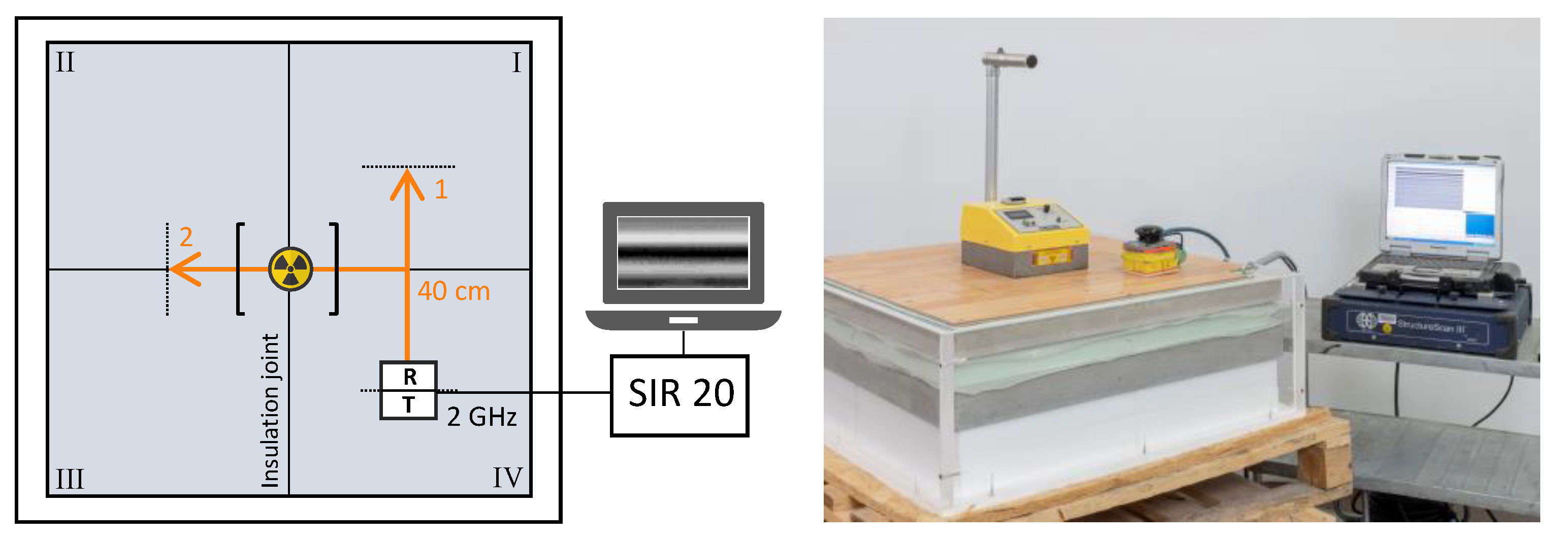
The GPR measurements were carried out with the SIR 20 from GSSI and a 2 GHz antenna pair (bandwidth 1 GHz to 3 GHz) in common-offset configuration. As shown in Figure 6, the ground-coupled antenna pair is moved along two defined 40 cm survey lines that run from quadrant IV to I (1) and along the insulation joint (2). These joints were present for EP, XP, and GW, though not for the fine-grained PS. With 250 scans/meter, each survey line includes 100 A-scans to form one B-scan. An A-scan contains 512 samples covering a 11 ns time window.
Furthermore, each floor construction was investigated with a Troxler neutron probe placed in the setup center. To reduce the influence of individual deviations, 10 successive measurements with a respective time interval of 15 seconds were averaged.
2.5. Feature Extraction
2.5.1. A-Scan Features
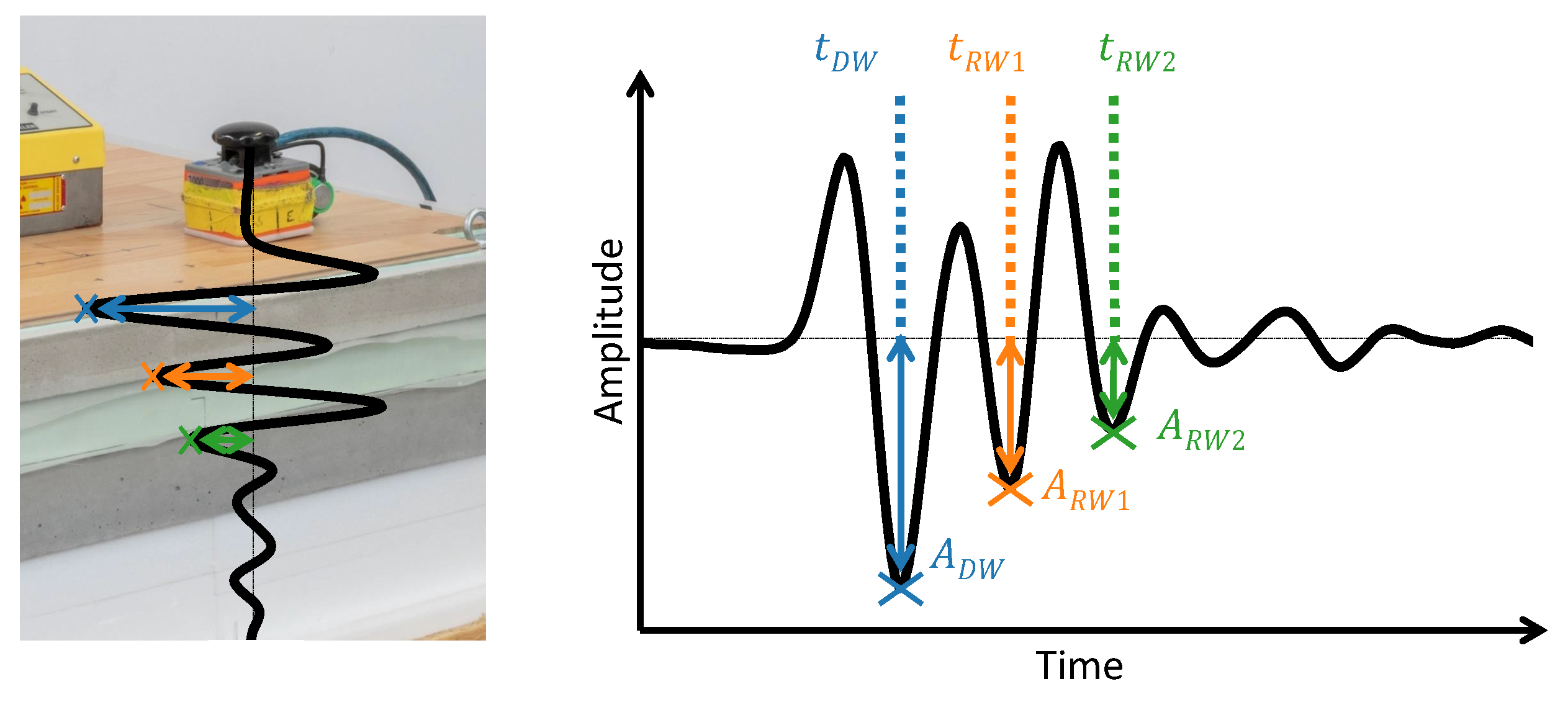
As discussed in Section 1.1 previously, there are several signal features enabling the measurement of water with GPR. Before presenting the ones chosen in this work, it is important to understand the typical signal shapes that occur on layered floor constructions. Figure 7 gives an exemplary A-scan showing three prominent amplitude peaks and their respective origin in the setup. Since the direct wave () partly travels through the superficial ground, it is influenced by the underlying nearest materials, here by the floor cover and the screed. The first reflection arises from the border between screed and insulation and is mostly recognized in the second dominant amplitude peak . After that, shows the second reflection’s amplitude, originating from the insulation-concrete interface below.
All described reflection waves can interfere, especially for dry or thin layers, where resulting higher velocities or short traveling paths impede a clear separation in time. This is also why quantitative statements about actual water content cannot be reliable for such layered floor constructions. However, classifying the investigated scenarios is still possible and will be performed with the following signal features:
|
The presented signal features cover all relevant signal parts, with insulation damage mostly influencing the second and first reflection and screed damage causing variations in the first reflection and the direct wave. However, the same features are also influenced by underlying layer thicknesses and different material types. Therefore, another preprocessing step is needed to overcome these construction-specific dependencies, which will be achieved by the B-scan features presented in the following section.
2.5.2. B-Scan Features
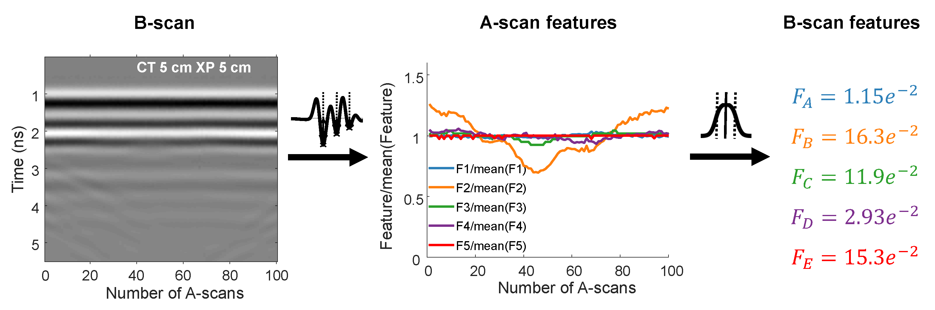
To achieve a damage classification independent of the underlying floor construction, we calculate the following scalar statistical values for each A-scan feature vector to , each including the respective feature elements to for all 100 A-Scans within one B-scan.
- Feature : Standard deviation of
- Feature : Standard deviation of
- Feature : Span of
- Feature : Standard deviation of
- Feature : Span of
These measures for statistical distributions along a recorded survey line are motivated by the assumption that water damage often shows inhomogeneous deviations inside the respective B-scan. Such deviations can also be suitable to evaluate the spatial continuity of present damage. Both findings were generally recognized during our studies and will be discussed in the results Section 3. For the lower resolved frequency features, the span is expected to achieve better variance compared to the standard deviation, which works well on amplitude features with a higher resolution and range of values.
Figure 8 summarizes the discussed processing steps including the extraction of A-scan feature vectors out of B-scans and the following reduction to scalar B-scan features. The values shown for to are derived from the depicted A-scan feature plots (normalized by their means). They do not represent the actual values that were used for classification, since those were standardized with the StandardScaler function from the Scikit-Learn library. It does a mean removal for all features and scales them to unit variance, which is usually required by the classifiers discussed in Section 2.6. Regarding the magnitudes of amplitude, time, and frequency values, which are widely apart from each other, this step is necessary to avoid a baseless and unwanted dominance of certain features during the training process.
2.5.3. Feature Selection
The choice of this specific A- and B-scan feature set was made based on the achieved scores using the univariate feature selection method SelectKBest from the Scikit-Learn library in Python [27]. Using the f_classif scoring function, it estimates the degree of linear dependency between random variables (here, the features and damage scenario) by using the F-test. The five features presented before performed best in a set of 22 potential features including amplitude, time, and frequency values/ratios of each relevant reflection type in Figure 7. To avoid the use of insufficient input variables, which would impede efficient computation, only these five features were used to train the classifiers (next section), and all others were discarded. The respective scores of the chosen feature set will be shown in Section 3.2.
2.6. Classification of Damage Scenarios
With 84 different floor constructions for each of the three scenarios and two survey lines measured, a data set of 504 B-scans was produced, from which the features mentioned above were extracted. With this data, we trained the following four classifiers in standard configuration (default parameters only), which are all included in the Scikit-Learn library. The default parameters can be found in the respective documentation (e.g., default kernel of SVM: radial basis function):
- Multinomial logistic regression (MLR)
- Random forest (RF)
- Support vector machine (SVM)
- Artificial neural network (ANN)
The ANN consisted of two hidden layers with five neurons each (according to the number of features). To get a statistical comparability of the accuracies achieved, a k = 20-fold cross-validation was applied for all classifiers using the cross_val_score function from Scikit-Learn. Here, the parameter cv (cross-validation generator) was defined with ShuffleSplit(n_splits = 20, test_size = 0.2, random_state = 0) which produces 20 random splits of training and test data sets with a size of 80% and 20%, respectively. All classifiers were cross-validated with the same set of splits, which includes 20 consecutive training and test procedures for each classifier. The results were then statistically evaluated (mean and standard deviation) and are shown in Section 3.2. However, before discussing the classification, an impression of the collected data shall be given with exemplary measurement results from the experiments.
3. Results
3.1. Measurements at Modular Specimen
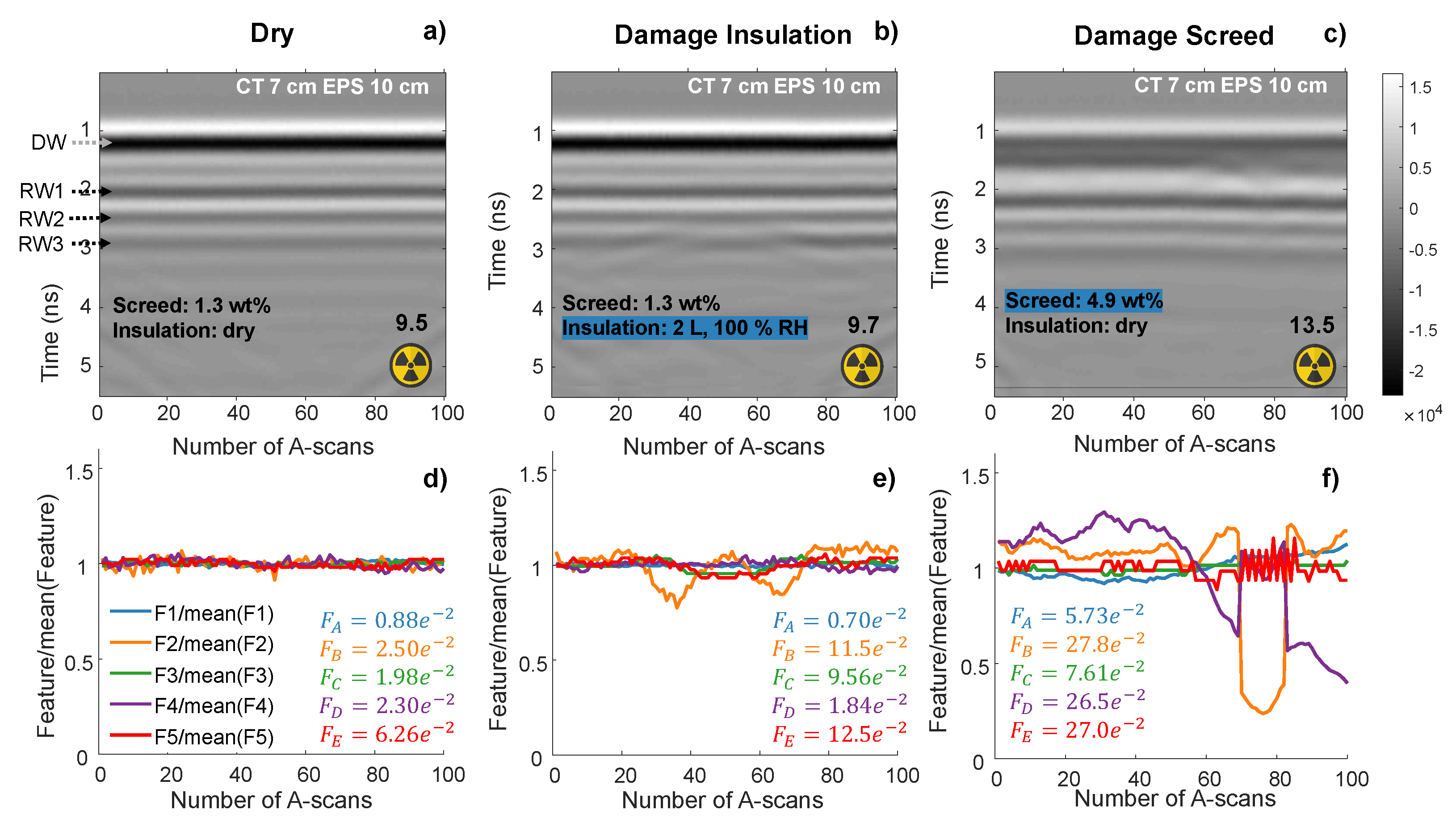
Figure 9 and Figure 10 show the measurement results of all three scenarios at one respective floor construction. The first covers the configuration of a 7 cm CT screed combined with a 10 cm EPS insulation. The B-scans on top also contain text information about the underlying moisture states of screed and insulation, as well as the performed neutron probe measurement. All exemplary radar results were collected along survey line 1 (see Figure 6).
According to the general assumption mentioned in Section 2.5.2, the dry measurement in (a) has a homogeneous reflection pattern, whereas the two damage scenarios in (b) and (c) present clear deviations at specific time-spans. For the insulation damage in (b), we see amplitude changes in the second (RW2) and third (RW3) reflection around 2.5 ns to 3 ns, which come from the affected layer. Water added to EPS usually gathers inside the insulation joints, and from there, it slowly penetrates the material. Therefore, the areas of higher attenuation were located horizontally around the survey line’s center, where the joint is crossed. These deviations become even clearer by considering the respective A-scan feature vector plots below each B-scan. Compared to the relatively flat lines for the dry measurement in (d), () particularly shows significant variations in (e), which is also captured by an increased standard deviation (). These deviations are not immediately recognizable in the B-scan, since the third reflection RW3 shows a more significant variance. Insulation of 10 cm thickness usually developed two reflections, whereby the latter and therefore third reflection was not covered by the used feature set. However, due to their interference, RW2 also experienced a change in amplitude and is therefore suitable for recognizing damage. Since the neutron probe is more sensitive to moisture closer to its radiation source, a small amount of water inside the insulation is not sufficient to cause a significant increase.
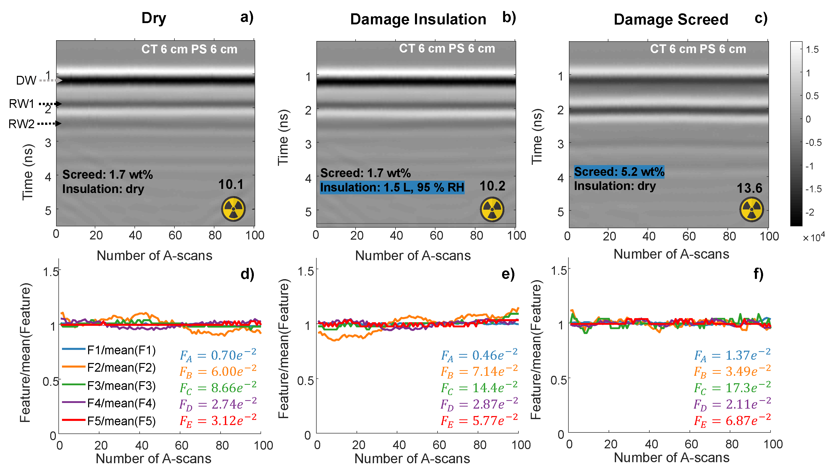
In the case of screed damage in (c), the water induces deviations which appear in earlier time-spans, like in the direct wave DW or the first reflection RW1. As shown in Figure 5, all screed samples were poured from above, which is why the DW experiences a significant drop in its amplitude compared to other scenarios. is especially sensitive to superficial material properties and is therefore an appropriate feature to recognize flooding damage. In this case, being the ratio of and shows a high dynamic in (f). This is also because an unexpected reflection occurs at around 1.4 ns right after the direct wave, which was not present in other scenarios. The reason could be a steep water gradient providing a strong permittivity contrast and therefore a new reflector. This assumption is supported by the highest NMR amplitude measured for the 7 cm CT among all screeds, which was around 90 at the sample’s surface. The other screeds had values of around 60 and did not show an extra reflection (compare Figure 10). Here, the new reflection at around 1.4 ns is interpreted as RW1, whereby the former RW1, originating from the screed bottom, is then seen as RW2. After a decrease of between A-scans 50 and 65, it completely disappears between 70 and 80, causing a shift in reflection-counting. This leads to dominant jumps for and , which cause an increased standard deviation and support the feature’s sensitivity for water-induced deviations. The neutron probe is also capable of recognizing the increased moisture content with a difference of 4 digits compared to the dry measurement.
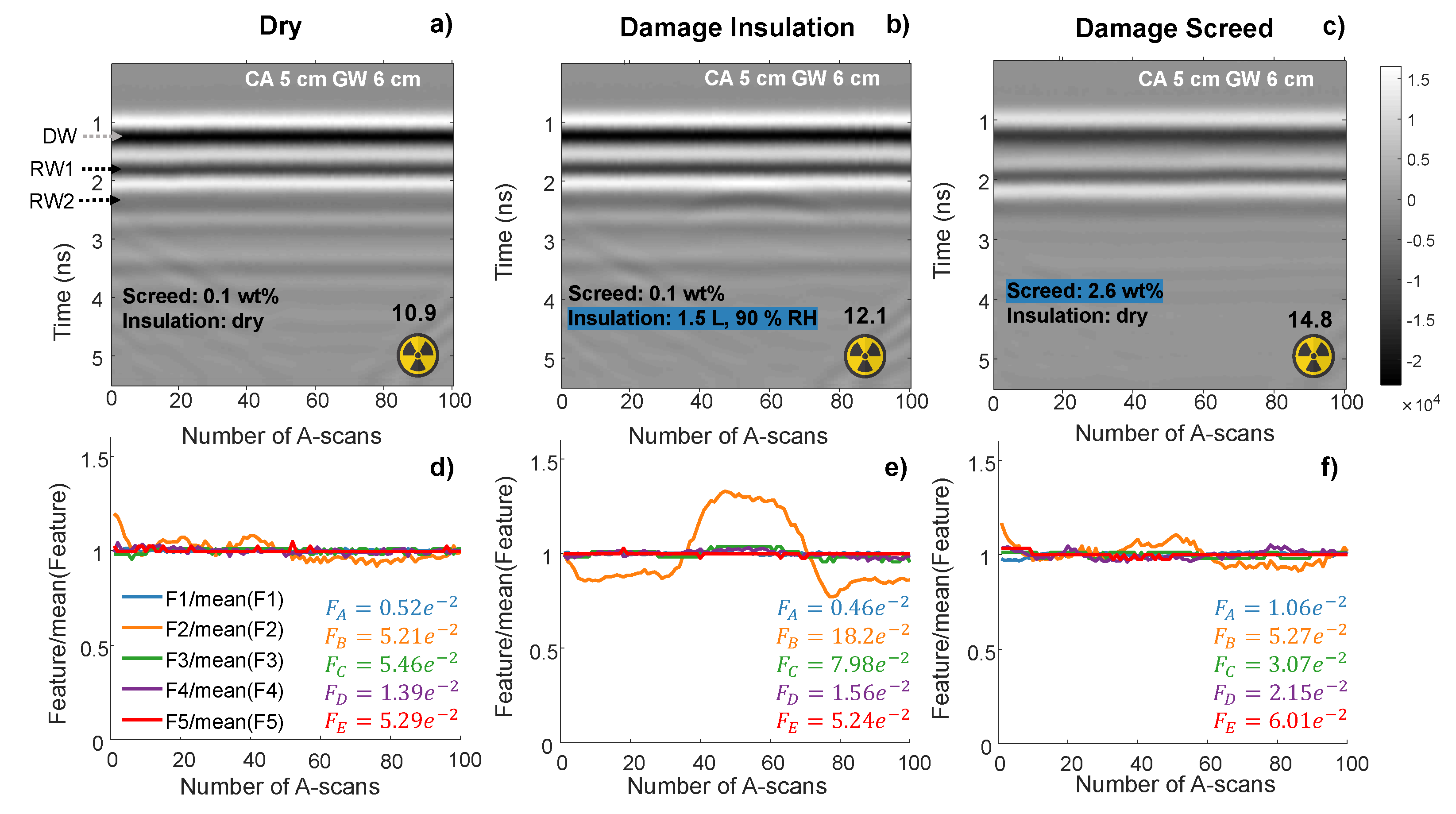
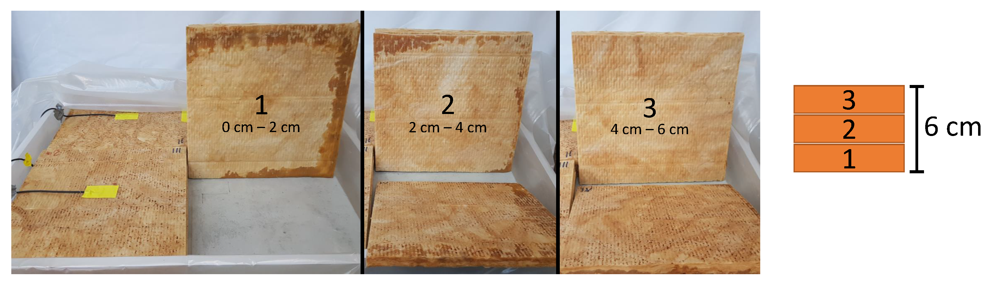
Figure 10 gives another example of a 5 cm CA screed and 6 cm GW floor construction. As before, the dry scenario in (a) shows a flat reflection pattern compared to notable deviations in the second reflection caused by a damaged insulation (b). Like with EPS, the water tended to accumulate in the joints between the GW plates and was slowly absorbed by the material. In this case, it formed a stronger permittivity contrast on the insulation’s bottom, which resulted in an increased reflection amplitude in the survey line’s center (see Equation (2)). This gets especially clear by considering Figure 11, in which parts of the GW insulation (measured by survey line 1) are shown. As all three plates were flipped by 90 degrees, the bottom edge belongs to the insulation joint between quadrants IV and I. The fact that only the first and lowest plate 1 shows marks of water ingress at this specific edge underlines the explanation of a strong permittivity contrast, which forms a thin reflector above the concrete plate. In this case, the neutron probe measures a slight increase due to an overall lower depth of the setup.
Another interesting difference to the example before can be seen in the damaged screed scenario (c), which is even more representative for the whole measured data set. Like with all other screeds (except the 7 cm CT) the induced moisture damages appear comparatively homogeneous and do not show the expected deviations. This can be explained by an evenly distributed moisture gradient throughout the whole sample. The most dominant influence is the overall reduced amplitude for DW, RW1, and RW2, which becomes clear by comparing the dry scenario. However, it is not a clear indication for water without this prior knowledge. Nevertheless, by considering the values of , and in (f), small increases can be registered, which might be sufficient to recognize the damage by trained classifiers. The validity of this statement shall be reviewed in the following section. Again, the screed damage is more visible for the neutron probe than moisture in the insulation layer.
3.2. Damage Scenario Classification
Table 2 shows the achieved mean accuracies with the standard deviation of all trained classifiers mentioned in Section 2.6. By using the features presented in Section 2.5, all algorithms were capable of correctly recognizing 84.3% to 88.3% of the considered damage scenarios, without further knowledge about the underlying material or layer thickness. With regard to the broad variations considered in this data set, these accuracies are quite satisfying. To provide a better understanding of the presented results, Figure 12 shows confusion matrices containing each used classifier for the individual layer thicknesses of insulation and screed.
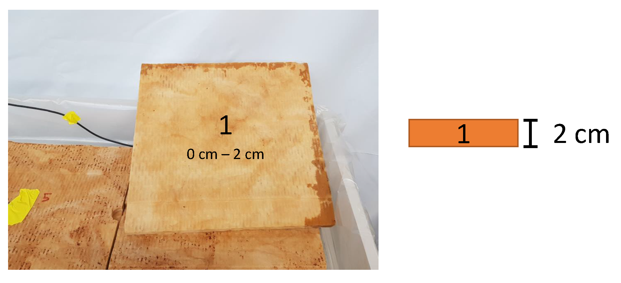
For a perfect classification with 100% accuracy, all confusion matrix cells (entries) except the main diagonal would be zero, which means that every scenario would have been classified correctly. Knowing that, the highest deviation of that perfect case gets immediately visible in Figure 12, which lies in the mid column of the top left matrix. It shows that more than half of the measured scenarios with a damaged insulation of 2 cm thickness were classified as dry. This can be explained by the low amount of water (around 0.5 L), that was necessary to cause relative humidities above 80%. Especially for GW and PS, the inserted water was absorbed by the outer edges and did not penetrate into measured areas. As a reference, Figure 13 again shows the flipped GW plate after the measurement with no signs of water ingress on the bottom edge (insulation joint between quadrant IV and I). Due to the significant number of unaffected B-scans, the classification results in Table 2 also show the accuracies for the excluded 2 cm insulation. All classifiers achieved a higher score and comparable standard deviations.
Additionally, for insulations of 6 cm thickness which only included GW and PS, the respective confusion matrix contains 8.3% to 37.5% false-negatives for damaged insulations. Since the GW of 6 cm already showed a measurable influence in Figure 10 and Figure 11, the wrongly classified scenarios are located in the PS data set. In fact, survey line 1 for PS of 6 cm thickness presents a smooth reflection pattern, which is exemplarily shown in Figure 14b). Unfortunately, the structure of PS did not allow referencing pictures like for GW; however, the similarity between dry and damaged insulation suggests that no water penetrated in the measured area.
In general, most of the wrong classifications are false-negatives, which are represented by entries left of the main diagonals. Besides the mentioned reasons for damaged insulations, the damaged screed scenario also shows around 5% to 20% of measurements that were classified as dry in nearly every confusion matrix. With regard to the mostly homogeneous reflection patterns shown in Figure 10 and Figure 14, these results are rather satisfying. It shows that even the slight deviations in , and , as discussed in the previous section, are mostly sufficient to recognize the considered screed damages.
Overall, the four used classifiers achieved similar accuracies in all matrix entries. Only the damaged screed scenario reveals a more significant trend with a comparatively poorly-performing SVM, while ANN shows the best results.
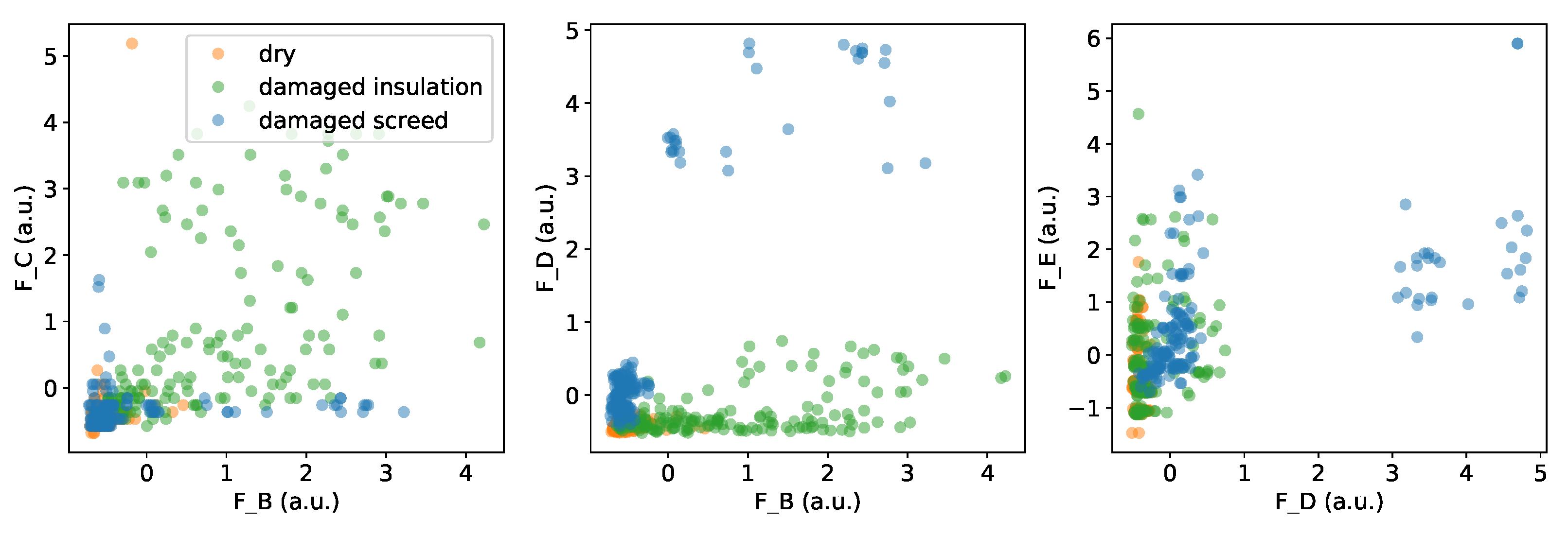
Looking at the achieved scores of each extracted feature can give a better insight into the data’s structure and their decisive components. Table 3 points out as the best-performing feature, followed by and .
The reasons for these scores become clearer by considering the selected scatter plots in Figure 15 with standardized values. Combining the best-performing, RW2-related features and shows a good separation of the damaged insulation scenario with a broad distribution of possible values. However, due to the discussed appearance of smooth reflection patterns, the damaged screed is mostly indistinguishable from the dry scenario. In this case, features regarding DW and RW1 are obviously more decisive, which can be seen by a better separation in the middle and left scatter plot. However, the separation is not that clear as for the damaged insulation with and , which explains the comparatively lower scores. The blue outliers belong to the 7 cm CT screed shown in Figure 9, where the extra reflector caused an unusually strong deviation in .
4. Discussion
The results show that the proposed method regarding the horizontal distribution of specific A-scan features in one B-scan is suitable to classify moisture damages in unknown floor constructions. In a data set of 504 B-scans covering 252 different experimental setups, 84.3% to 88.3% of the scenario’s dry, damaged insulation, and damaged screed were recognized correctly by the trained classifiers. A closer investigation of the produced false-negatives often revealed the measurement of undamaged areas which underlines the method’s sensitivity and suggest even higher accuracies. In particular, the combination of amplitude and frequency features covering all relevant reflections in the GPR signal contributed to the successful results. Therefore, this study generally proposes an enhanced use of multivariate data analysis when performing moisture measurements with GPR.
The presented method also worked well as a supporting procedure for the neutron probe. In particular, moisture inside the insulation layer was mostly undetected by the sole use of the radiation measurement, whereas GPR achieved a satisfying sensitivity.
Since the data set only contained laboratory measurements under controlled conditions, the method still needs to be validated in practical on-site investigations of real damage cases. Here, unknown parameters like an unstable layer thickness or obstructive floor heating pipes could lead to misinterpretations which might produce an increased number of false-positive classifications. Upcoming works by the authors will address these questions. If satisfying accuracies can be achieved, the method will be capable of significantly reducing the need for destructive drilling cores to classify underlying damage scenarios, and therefore cut the costs of renovations.
Further, potential optimizations could be investigated regarding the classifiers’ configurations, since only default parameters have been used so far. In addition, the use of deep learning (ANN) to automatically extract novel, relevant features out of radargrams (b-scans as input parameter) can be examined with the obtained dataset.
Author Contributions
Conceptualization, T.K., C.S., T.R. and S.K.; methodology, T.K., C.S., T.R. and S.K.; software, T.K.; validation, T.K.; formal analysis, T.K.; investigation, T.K.; resources, C.S., T.R. and S.K.; data curation, T.K.; writing—original draft preparation, T.K.; writing—review and editing, C.S. and S.K.; visualization, T.K.; supervision, C.S. and S.K.; project administration, C.S.; funding acquisition, C.S. and S.K. All authors have read and agreed to the published version of the manuscript.
Funding
This research received no external funding.
Acknowledgments
The authors would like to thank Thomas Kind and Christian Köpp for their helpful comments on the text. For their support in producing the screed samples, gratitude is owed to Hans-Carsten Kühne and Frank Haamkens.
Conflicts of Interest
The authors declare no conflict of interest.
Abbreviations
The following abbreviations are used in this manuscript:
| ANN | Artificial neural network |
| CA | Anhydrite |
| CE | Civil engineering |
| CT | Cement |
| DAQ | Data acquisition |
| GPR | Ground penetrating radar |
| DW | Direct Wave |
| EM | Electromagnetic |
| EP | Expanded polysterene |
| GW | Glass wool |
| MLR | Multinomial logistic regression |
| NMR | Nuclear magnetic resonance |
| PS | Perlites |
| R | Receiver |
| RF | Random forest |
| RW | Reflection Wave |
| STFT | Short-time Fourier transform |
| SVM | Support vector machine |
| T | Transmitter |
| XP | Extruded polysterene |
References
- GDV. Annual of Gesamtverband der Deutschen Versicherungswirtschaft e.V. 2019. Available online: https://www.gdv.de/de/zahlen-und-fakten/versicherungsbereiche/wohngebaeude-24080 (accessed on 20 July 2021).
- Chanasky, D.S.; Naeth, M.A. Field measurement of soil moisture using neutron probes. Can. J. Soil Sci. 1996, 76, 317–323. [Google Scholar] [CrossRef]
- Huisman, J.A.; Hubbard, S.S.; Redman, J.D.; Annan, A.P. Measuring Soil Water Content with Ground Penetrating Radar: A Review. Vadose Zone J. 2003, 2, 476–491. [Google Scholar] [CrossRef]
- Slater, L.; Comas, X. The Contribution of Ground Penetrating Radar to Water Resource Research. In Ground Penetrating Radar: Theory and Applications; Elsevier: Amsterdam, The Netherlands, 2009. [Google Scholar]
- Saarenketo, T.; Scullion, T. Road evaluation with ground-penetrating radar. J. Appl. Geophys. 2000, 43, 119–138. [Google Scholar] [CrossRef]
- Klysz, G.; Balayssac, J.P. Determination of volumetric water content of concrete using ground-penetrating radar. Cem. Concr. Res. 2007, 37, 1164–1171. [Google Scholar] [CrossRef]
- Grote, K.; Hubbard, S.; Harvey, J.; Rubin, Y. Evaluation of infiltration in layered pavements using surface GPR reflection techniques. J. Appl. Geophys. 2005, 57, 129–153. [Google Scholar] [CrossRef]
- Laurens, S.; Balayssac, J.P.; Rhazi, J.; Klysz, G.; Arliguie, G. Non-destructive evaluation of concrete moisture by GPR: Experimental study and direct modeling. Mater. Struct. 2005, 38, 827–832. [Google Scholar] [CrossRef]
- Lai, W.L.; Kou, S.C.; Tsang, W.F.; Poon, C.S. Characterization of concrete properties from dielectric properties using ground-penetrating radar. Cem. Concr. Res. 2009, 39, 687–695. [Google Scholar] [CrossRef]
- Kurz, F.; Sgarz, H. Measurement of Moisture Content in Building Materials using Radar Technology. In Proceedings of the International Symposium Non-Destructive Testing in Civil Engineering (NDT-CE), Berlin, Germany, 15–17 September 2015. [Google Scholar]
- Klewe, T.; Strangfeld, C.; Kruschwitz, S. Review of moisture measurements in civil engineering with ground penetrating radar—Applied methods and signal features. Constr. Build. Mater. 2021, 278, 122250. [Google Scholar] [CrossRef]
- Davis, J.L.; Annan, A.P. Electromagnetic Detection of Soil Moisture: Progress Report I. Can. J. Remote Sens. 1977, 3, 76–86. [Google Scholar] [CrossRef]
- Soutsos, M.N.; Bungey, J.H.; Millard, S.G.; Shaw, M.R.; Patterson, A. Dielectric properties of concrete and their influence on radar testing. NDT&E Int. 2001, 34, 419–425. [Google Scholar] [CrossRef]
- Daniels, D.J. Ground Penetrating Radar, 2nd ed.; The Institution of Engineering and Technology: London, UK, 2007. [Google Scholar]
- Annan, A.P. Electromagnetic Principles of Ground Penetrating Radar. In Ground Penetrating Radar: Theory and Applications; Jol, H.M., Ed.; Elsevierr: Amsterdam, The Netherlands, 2009; Chapter 1; pp. 4–38. [Google Scholar]
- Bohren, C.; Huffman, D. Absorption and Scattering of Light by Small Particles; Wiley: Hoboken, NJ, USA, 1983. [Google Scholar]
- Debye, P.J.W. Polar molecules. J. Soc. Chem. Ind. 1929, 48, 1036–1037. [Google Scholar] [CrossRef]
- Cole, K.S.; Cole, R.H. Dispersion and Absorption in Dielectrics I. Alternating Current Characteristics. J. Chem. Phys. 1941, 9, 341–351. [Google Scholar] [CrossRef] [Green Version]
- Kaatze, U. Complex permittivity of water as a function of frequency and temperature. J. Chem. Eng. Data 1989, 34, 371–374. [Google Scholar] [CrossRef]
- Balanis, C.A. Advanced Engineering Electromagnetics, 2nd ed.; John Wiley & Sons: Somerset, NJ, USA, 2012. [Google Scholar]
- Yelf, R. Where is true time zero? In Proceedings of the Tenth International Conference on Ground Penetrating Radar, Delft, The Netherlands, 21–24 June 2004. [Google Scholar] [CrossRef]
- Coppock, J.B.M.; Cookson, E.D. The effect of humidity on mould growth on constructional materials. J. Sci. Food Agric. 1951, 2, 534–537. [Google Scholar] [CrossRef]
- ASTM D2216-19. Standard Test Methods for Laboratory Determination of Water (Moisture) Content of Soil and Rock by Mass. ASTM 2019, 4, 8. [Google Scholar]
- Blümich, B.; Blümler, P.; Eidmann, G.; Guthausen, A.; Haken, R.; Schmitz, U.; Saito, K.; Zimmer, G. The NMR-mouse: Construction, excitation, and applications. Magn. Reson. Imaging 1998, 16, 479–484. [Google Scholar] [CrossRef]
- Blümich, B.; Perlo, J.; Casanova, F. Mobile single-sided NMR. Prog. Nucl. Magn. Reson. Spectrosc. 2008, 52, 197–269. [Google Scholar] [CrossRef]
- Lai, W.L.; Kind, T.; Kruschwitz, S.; Wöstmann, J.; Wiggenhauser, H. Spectral absorption of spatial and temporal ground-penetrating radar signals by water in construction materials. NDT&E Int. 2014, 67, 55–63. [Google Scholar] [CrossRef]
- Pedregosa, F.; Varoquaux, G.; Gramfort, A.; Michel, V.; Thirion, B.; Grisel, O.; Blondel, M.; Prettenhofer, P.; Weiss, R.; Dubourg, V.; et al. Scikit-learn: Machine Learning in Python. J. Mach. Learn. Res. 2011, 12, 2825–2830. [Google Scholar]
Figure 1.
Principle of GPR. Multiple A-scans collected along a survey line form a B-scan.

Figure 2.
Schematic of the work steps presented in Section 2 divided by their respective subsections.
Figure 2.
Schematic of the work steps presented in Section 2 divided by their respective subsections.

Figure 3.
Modular test specimen with screed, insulation, and concrete base layer.

Figure 4.
Evaluation of the resulting insulation damage through the use of embedded humidity sensors.
Figure 4.
Evaluation of the resulting insulation damage through the use of embedded humidity sensors.

Figure 5.
NMR measurements showing the depth-resolved moisture distribution during the saturation process of the 5 cm CT (left) and CA (right) screed.
Figure 5.
NMR measurements showing the depth-resolved moisture distribution during the saturation process of the 5 cm CT (left) and CA (right) screed.

Figure 6.
Measurement procedure with 40 cm long radar survey lines 1 and 2. The neutron probe is placed in the center of the construction.
Figure 6.
Measurement procedure with 40 cm long radar survey lines 1 and 2. The neutron probe is placed in the center of the construction.

Figure 7.
Exemplary A-scan with three prominent amplitudes influenced by present material interfaces.
Figure 7.
Exemplary A-scan with three prominent amplitudes influenced by present material interfaces.

Figure 8.
Processing steps to extract A- and B-scan features.

Figure 9.
Measurements at a 7 cm CT and 10 cm EPS floor construction for the scenarios: (a) Dry, (b) damage insulation, and (c) damage screed. The bottom (d–f) shows the respective A-scan vector plots for each B-scan (top).
Figure 9.
Measurements at a 7 cm CT and 10 cm EPS floor construction for the scenarios: (a) Dry, (b) damage insulation, and (c) damage screed. The bottom (d–f) shows the respective A-scan vector plots for each B-scan (top).

Figure 10.
Measurements at an 7 cm CA and 6 cm GW floor construction for the scenarios: (a) dry, (b) damage insulation and (c) damage screed. The bottom (d–f) shows the respective A-scan vector plots for each B-scan (top).
Figure 10.
Measurements at an 7 cm CA and 6 cm GW floor construction for the scenarios: (a) dry, (b) damage insulation and (c) damage screed. The bottom (d–f) shows the respective A-scan vector plots for each B-scan (top).

Figure 11.
Water ingress (dark dyeing) in the 6 cm GW insulation. The pictures show the respective bottom of each used insulation plate (40 cm × 40 cm × 2 cm) in quadrant IV.
Figure 11.
Water ingress (dark dyeing) in the 6 cm GW insulation. The pictures show the respective bottom of each used insulation plate (40 cm × 40 cm × 2 cm) in quadrant IV.

Figure 12.
Combined confusion matrices for the individual insulation (green) and screed (gray) thicknesses considered in the experiment. The classifier’s accuracies within one cell are presented in the same order as in Table 2. Rows and columns include the actual and the predicted (⌃) scenario, respectively. The blue confusion matrix summarizes the overall accuracies for each scenario.

Figure 13.
Water ingress (dark dyeing) in the 2 cm GW insulation. The picture shows the bottom of the used insulation plate (40 cm × 40 cm × 2 cm) in quadrant IV.
Figure 13.
Water ingress (dark dyeing) in the 2 cm GW insulation. The picture shows the bottom of the used insulation plate (40 cm × 40 cm × 2 cm) in quadrant IV.

Figure 14.
Measurements at a 6 cm CT and 6 cm PS floor construction for the scenarios: (a) dry, (b) damaged insulation, and (c) damaged screed. The bottom (d–f) shows the respective A-scan vector plots for each B-scan (top).
Figure 14.
Measurements at a 6 cm CT and 6 cm PS floor construction for the scenarios: (a) dry, (b) damaged insulation, and (c) damaged screed. The bottom (d–f) shows the respective A-scan vector plots for each B-scan (top).

Figure 15.
Scatter plots showing the feature combination of & (left), & (middle) and & (right).


Table 1.
Used materials and layer thicknesses for the screed (top) and insulation layer (bottom).
| Material | Thickness D [cm] | Density [g·cm−3] | Porosity * [%] |
|---|---|---|---|
| Cement screed (CT) | 5, 6, 7 | 1.92 | 20.76 |
| Anhydrite screed (CA) | 5, 6, | 2.05 | 27.18 |
| Expanded polysterene (EP) | 2, 5, 7, 10 | 0.027 | - |
| Extruded polysterene (XP) | 2, 5, 7, 10 | 0.037 | - |
| Glass wool (GW) | 2, 6, 10 | 0.061 | - |
| Perlites (PS) | 2, 6, 10 | 0.092 | - |
* Measured with mercury intrusion porosimetry.
Table 2.
Statistical comparison (k = 20-fold cross-validation) of the achieved accuracies for all trained classifiers.
Table 2.
Statistical comparison (k = 20-fold cross-validation) of the achieved accuracies for all trained classifiers.
| Classifier | Accuracy (%) | Accuracy * (%) | ||
|---|---|---|---|---|
| Mean | Std | Mean | Std | |
| MLR | 86.4 | 3.0 | 89,7 | 3.1 |
| RF | 88.3 | 3.7 | 92.2 | 2.6 |
| SVM | 84.3 | 3.3 | 86.6 | 3.9 |
| ANN | 88.2 | 3.6 | 93.5 | 2.5 |
* Cases with insulation depth of D = 2 cm excluded.
Table 3.
Achieved scores of the applied B-scan features.
| Feature | Origin in A-Scan | Score |
|---|---|---|
| 0.61 | ||
| 1.0 | ||
| 0.95 | ||
| 0.48 | ||
| 0.41 |
Publisher’s Note: MDPI stays neutral with regard to jurisdictional claims in published maps and institutional affiliations. |
© 2021 by the authors. Licensee MDPI, Basel, Switzerland. This article is an open access article distributed under the terms and conditions of the Creative Commons Attribution (CC BY) license (https://creativecommons.org/licenses/by/4.0/).
Share and Cite
MDPI and ACS Style
Klewe, T.; Strangfeld, C.; Ritzer, T.; Kruschwitz, S. Combining Signal Features of Ground-Penetrating Radar to Classify Moisture Damage in Layered Building Floors. Appl. Sci. 2021, 11, 8820. https://doi.org/10.3390/app11198820
AMA Style
Klewe T, Strangfeld C, Ritzer T, Kruschwitz S. Combining Signal Features of Ground-Penetrating Radar to Classify Moisture Damage in Layered Building Floors. Applied Sciences. 2021; 11(19):8820. https://doi.org/10.3390/app11198820
Chicago/Turabian StyleKlewe, Tim, Christoph Strangfeld, Tobias Ritzer, and Sabine Kruschwitz. 2021. "Combining Signal Features of Ground-Penetrating Radar to Classify Moisture Damage in Layered Building Floors" Applied Sciences 11, no. 19: 8820. https://doi.org/10.3390/app11198820
Note that from the first issue of 2016, this journal uses article numbers instead of page numbers. See further details here.