Analyzing the Stability for the Motion of an Unstretched Double Pendulum near Resonance

Abstract

This work looks at the nonlinear dynamical motion of an unstretched two degrees of freedom double pendulum in which its pivot point follows an elliptic route with steady angular velocity. These pendulums have different lengths and are attached with different masses. Lagrange’s equations are employed to derive the governing kinematic system of motion. The multiple scales technique is utilized to find the desired approximate solutions up to the third order of approximation. Resonance cases have been classified, and modulation equations are formulated. Solvability requirements for the steady-state solutions are specified. The obtained solutions and resonance curves are represented graphically. The nonlinear stability approach is used to check the impact of the various parameters on the dynamical motion. The comparison between the attained analytic solutions and the numerical ones reveals a high degree of consistency between them and reflects an excellent accuracy of the used approach. The importance of the mentioned model points to its applications in a wide range of fields such as ships motion, swaying buildings, transportation devices and rotor dynamics.

1. Introduction

A dynamical system is a system dependent on time. It describes the time dependency of a point in space such as a hanging clock and a current of water in a pipe [1]. It can be used in a variety of domains, including mathematics, physics, chemistry, engineering in the construction of swaying buildings, biology, economics and medicine [2,3]. Since applied mechanics is considered as a section of physical science that describes a response of the bodies’ system, which started from rest or motion under the influence of external forces [4], it has been used in many fields of engineering, especially electrical and mechanical engineering, in the areas of engineering machines, rotor dynamics, pumps and compressors.

The nonlinear motion of a pendulum has piqued the interest of a number of researchers, e.g., [5,6,7,8,9]. Kyoung et al. [5] and Lee et al. [6] examined a chaotic response of a spring pendulum with two degrees of freedom (DOF). The multiple scales technique (MST) is utilized to solve the equations of motion (EOM). Moreover, they studied the bifurcation of the controlling system. In [7], the authors examined the response of the last pendulum using the MST. Additionally, the effects of internal and external resonance were studied. The impact of a higher-order approximation of an excited harmonically spring pendulum was examined in [8]. They compared the accuracy between the first and second approximation using the Lyapunov exponent method. In [9], the asymptotic and limiting phase trajectories (LPT) were applied to study the same problem in which MST and LPT were used to solve the governing system. The authors examined the impact of physical parameters on dynamical motion with the aid of LPT to describe any variation of the considered model. The analytical solutions were verified by comparing them with the numerical ones. From another perspective, the transversal tuned absorber of an exciting spring pendulum was used to control the system vibrations due to the existence of influential excitation forces, e.g., [10,11]. A numerical investigation of the positive impact of the absorber on the dynamical behaviour is presented. The asymptotic solutions of a nonlinear motion of a pendulum-type were investigated in [12] utilizing the MST, in which the trigonometric functions were approximated in the EOM using polynomial approximation. In [13], the authors explored a 2-DOF spring pendulum in an inviscid fluid flow. Approximate solutions were gained using the same approach as previously up to the second order of approximation. Resonance curves, steady-state solutions and stability of motion were examined and represented graphically. The dynamic response of a spring pendulum was investigated in [14,15], in which the MST was applied to gain the asymptotic solutions of the analyzed systems. A generalization of this work is found in [16], where the authors studied a damped spring motion that follows an elliptic route. An extension of this research was found in [17,18], when the suspension point was travelling in the same direction, with a constant angular velocity of a linear spring and nonlinear one, respectively. The case of the attached tuned absorber with the spring was investigated in [19]. The derived EOM were solved analytically, and the modulations equations were acquired in the line of the considered resonance cases. The time histories and the resonance curves were plotted to reveal the impact of the body’s parameters on the motion. Another trajectory for the motion of the pivot point was considered in [20], in which the authors elaborated the dynamical motion of the 2-DOF damped elastic pendulum in a Lissajous curve. Conversely, the plane motion of the 3-DOF rigid body pendulum with a fixed suspension point was investigated in [21]. The latter two works are generalized in [22] when the supported point of the damped rigid body moved in a path similar to the Lissajous curve. The authors discussed all the possible amplitudes of the steady-state solutions for different parameters of the considered models in light of the perturbation approach used. All cases of resonance were categorized, and the case of simultaneously parametric and primary resonances was examined. A plane motion of a triple pendulum system was investigated in [23,24] in the presence of free conditions. The natural frequencies of this model are studied in [23], while the recurrence plot method was used in [24] to achieve the required solutions of the derived EOM.

This paper studied the dynamical motion of the 2-DOF double pendulum system with two different massless rods of constant lengths. It is assumed that its supported point moves along an elliptical path with a stationary angular speed. The governing EOM were derived using Lagrange’s equations and were solved utilizing the MST up to the third order of approximation. The solvability conditions of the solutions at the steady state were determined. The resonance cases were obtained and categorized, in which the case of primary external resonance was examined. The curves of the time histories of the attained solutions and resonance ones were plotted with various selected values of the used parameters to reveal the good impact of these parameters on the dynamical behaviour of the investigated system. The analytical results were compared with the numerical calculations to reflect the high matching between them. The nonlinear stability analysis was used to investigate the characteristics of the dynamical motion. The importance of the model selected lies in its diverse set of applications in different fields, for example, in swaying buildings.

2. Dynamical Modelling

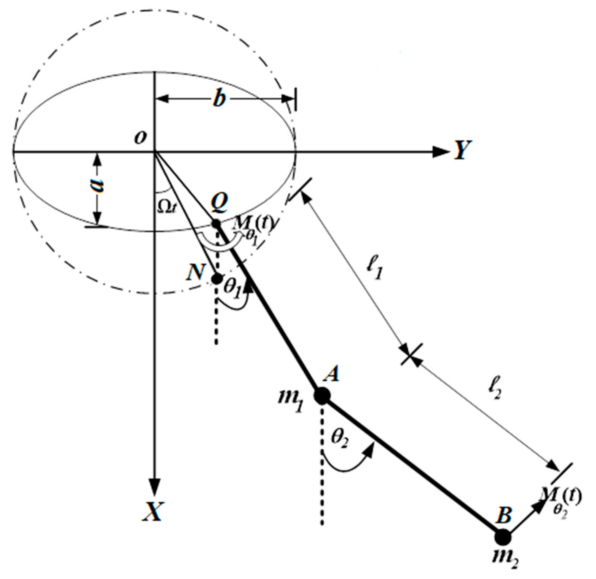
Nonlinear vibration of the 2-DOF dynamical paradigm consisting of a double pendulum is investigated in the present study. It is supposed that the supported point $Q$ of the modelling system travels along an elliptic track with lengths $2b$ and $2a$ of its major and minor axes, respectively. This point is connected with the double pendulum with constant lengths ${\mathcal{\ell }}_1$ and ${\mathcal{\ell }}_2$, see Figure 1. Consider $N$ to be the compatibility point of $Q$ on the spare circle $b$, in which it moves with a constant angular speed $\Omega$. The kinematics Cartesian coordinates of $Q$ are written in the following form:

$$x_Q=a\cos (\Omega t),\hspace{0.17em}\hspace{0.17em}\hspace{0.17em}\hspace{0.17em}\hspace{0.17em}\hspace{0.17em}{y}_Q=b\sin (\Omega t).$$

(1)

The kinetic and potential energies of the system can be expressed as follows:

$$\begin{array}{l}T=\frac{1}{2}(m_1+m_2){\Omega }^2\{a^2{\sin }^2(\Omega t)+b^2{\cos }^2(\Omega t)\}+(m_1+m_2)\Omega {\mathcal{\ell }}_1{\dot{\theta }}_1\\ \hspace{0.17em}\hspace{0.17em}\hspace{0.17em}\hspace{0.17em}\hspace{0.17em}\times \{a\sin (\Omega t)\sin {\theta }_1+b\cos (\Omega t)\cos {\theta }_1\}+m_2\Omega {\mathcal{\ell }}_2{\dot{\theta }}_2\{a\sin (\Omega t)\sin {\theta }_2\\ \hspace{0.17em}\hspace{0.17em}\hspace{0.17em}\hspace{0.17em}\hspace{0.17em}+b\cos (\Omega t)\cos {\theta }_2\}+m_2{\mathcal{\ell }}_1{\mathcal{\ell }}_2{\dot{\theta }}_1{\dot{\theta }}_2\cos ({\theta }_1-{\theta }_2)+\frac{1}{2}{m}_2{\mathcal{\ell }}_2{}^2{\dot{\theta }}_2{}^2\hspace{0.17em}\hspace{0.17em}\hspace{0.17em}\\ \hspace{0.17em}\hspace{0.17em}\hspace{0.17em}\hspace{0.17em}\hspace{0.17em}+\frac{1}{2}(m_1+m_2){\mathcal{\ell }}_1{}^2{\dot{\theta }}_1{}^2,\\ V=-(m_1+m_2)g\{a\cos (\Omega t)+{\mathcal{\ell }}_1\cos {\theta }_1\}-m_{2}g{\mathcal{\ell }}_2\cos {\theta }_2\hspace{0.17em}.\end{array}$$

(2)

Here, $g$ is the gravity acceleration, ${\theta }_1$ and ${\theta }_2$ are the angles formed by the vertical and the line directed through $QA$ and $AB$, respectively, and the dots refer to the differentiation regarding the time $t$.

Consider a moment $M_{{\theta }_1}(t)=M_1\cos ({\Omega }_{1}t)$ at the point $Q,$ besides an external moment $M_{{\theta }_2}(t)=M_2\cos ({\Omega }_{2}t)$ that acts on the mass $m_2$, in which $({\Omega }_1,\hspace{0.17em}{\Omega }_2)$ and $(M_1,\hspace{0.17em}{M}_2)$ are the forcing frequencies and the amplitudes of $M_{{\theta }_1}(t)$ and $M_{{\theta }_2}(t)$, respectively.

Using Lagrange’s functions $L=T-V$, one can derive the governing EOM by using the following Lagrange’s equations of the second type:

$$\begin{array}{l}\frac{d}{dt}(\frac{\partial L}{\partial {\dot{\theta }}_1})-(\frac{\partial L}{\partial {\theta }_1\hspace{0.17em}})=Q_{{\theta }_1\hspace{0.17em}},\\ \frac{d}{dt}(\frac{\partial L}{\partial {\dot{\theta }}_2})-(\frac{\partial L}{\partial {\theta }_2\hspace{0.17em}})=Q_{{\theta }_2\hspace{0.17em}}\hspace{0.17em}.\end{array}$$

(3)

Here, ${\theta }_1$ and ${\theta }_2\hspace{0.17em}$ are the system’s generalized coordinates, and $Q_{{\theta }_1\hspace{0.17em}}$ and $Q_{{\theta }_2\hspace{0.17em}}$ are the generalized forces that have the following forms:

$$\begin{array}{l}{Q}_{{\theta }_1\hspace{0.17em}}=M_1\cos ({\Omega }_{1}t),\\ Q_{{\theta }_2\hspace{0.17em}}=M_2\cos ({\Omega }_{2}t).\end{array}$$

(4)

Let us consider the following frequencies and parameters:

$$\begin{array}{l}\hspace{0.17em}\hspace{0.17em}{\omega }_1{}^2=\frac{g}{{\mathcal{\ell }}_1},\hspace{0.17em}\hspace{0.17em}\hspace{0.17em}\hspace{0.17em}{\omega }_2{}^2=\frac{g}{{\mathcal{\ell }}_2}\hspace{0.17em},\hspace{0.17em}\hspace{0.17em}\hspace{0.17em}\hspace{0.17em}p=\frac{\Omega }{{\omega }_1}\hspace{0.17em},\hspace{0.17em}\hspace{0.17em}\hspace{0.17em}\hspace{0.17em}{p}_1=\frac{{\Omega }_1}{{\omega }_1},\hspace{0.17em}\hspace{0.17em}\hspace{0.17em}\hspace{0.17em}{p}_2=\frac{{\Omega }_2}{{\omega }_1}\hspace{0.17em},\\ \hspace{0.17em}\hspace{0.17em}{\omega }^2=\frac{{\omega }_2{}^2}{{\omega }_1{}^2}\hspace{0.17em},\hspace{0.17em}\hspace{0.17em}\hspace{0.17em}\hspace{0.17em}\hspace{0.17em}\mu =\frac{m_2{\mathcal{\ell }}_2}{(m_1+m_2){\mathcal{\ell }}_1}\hspace{0.17em},\hspace{0.17em}\hspace{0.17em}\hspace{0.17em}\hspace{0.17em}\alpha =\frac{a}{{\mathcal{\ell }}_1},\hspace{0.17em}\hspace{0.17em}\hspace{0.17em}\hspace{0.17em}\beta =\frac{b}{{\mathcal{\ell }}_1},\hspace{0.17em}\hspace{0.17em}\hspace{0.17em}\hspace{0.17em}\tau ={\omega }_1\hspace{0.17em}t,\\ \hspace{0.17em}\hspace{0.17em}{f}_1=\frac{M_1}{(m_1+m_2){\omega }_1{}^2{\mathcal{\ell }}_1{}^2}\hspace{0.17em},\hspace{0.17em}\hspace{0.17em}\hspace{0.17em}\hspace{0.17em}{f}_2=\frac{M_2}{m_2{\omega }_1{}^2{\mathcal{\ell }}_2{}^2}.\hspace{0.17em}\hspace{0.17em}\end{array}$$

Using (2), (3) and (4), we can obtain the EOM in the following dimensionless forms:

$$\begin{array}{l}{\ddot{\theta }}_1+p^2[\alpha \cos (pt)\sin {\theta }_1-\beta \sin (pt)\cos {\theta }_1]+\sin {\theta }_1+\mu {\ddot{\theta }}_2\cos {\theta }_1\cos {\theta }_2\\ +\mu {\ddot{\theta }}_2\sin {\theta }_1\sin {\theta }_2+\mu {\dot{\theta }}_2{}^2\sin {\theta }_1\cos {\theta }_2-\mu {\dot{\theta }}_2{}^2\sin {\theta }_2\cos {\theta }_1=f_1\cos (p_{1}t),\end{array}$$

(5)

$$\begin{array}{l}{\ddot{\theta }}_2+p^2{\omega }^2[\alpha \cos (pt)\sin {\theta }_2-\beta \sin (pt)\cos {\theta }_2]+{\omega }^2\sin {\theta }_2+{\omega }^2{\ddot{\theta }}_1\cos {\theta }_1\cos {\theta }_2\\ +{\omega }^2{\ddot{\theta }}_1\sin {\theta }_1\sin {\theta }_2-{\omega }^2{\dot{\theta }}_1{}^2\sin {\theta }_1\cos {\theta }_2+{\omega }^2{\dot{\theta }}_1{}^2\sin {\theta }_2\cos {\theta }_1=f_2\cos (p_{2}t).\end{array}$$

(6)

3. Analysis of the Solution

In this section, the MST is applied to solve the EOM (5) and (6) analytically up to the third order of approximation, aiming to obtain the solvability resonance conditions and the modulation equations. To achieve this goal, the trigonometric functions $\sin \phi ,\hspace{0.17em}\hspace{0.17em}\cos \phi ,\hspace{0.17em}\hspace{0.17em}\sin \gamma ,$ and $\cos \gamma$ can be approximated up to the third order using Taylor’s series. Therefore, Equations (5) and (6) can be rewritten in the forms:

$$\begin{array}{l}{\ddot{\theta }}_1+p^2\{\alpha \cos (pt)\hspace{0.17em}\hspace{0.17em}({\theta }_1-\frac{{\theta }_1{}^3}{6})\hspace{0.17em}\hspace{0.17em}-\beta \sin (p\hspace{0.17em}t)\hspace{0.17em}(1-\frac{{\theta }_1{}^2}{2})\hspace{0.17em}\}+\hspace{0.17em}\hspace{0.17em}\hspace{0.17em}({\theta }_1-\frac{{\theta }_1{}^3}{6})\hspace{0.17em}+\mu {\ddot{\theta }}_2\hspace{0.17em}(1-\frac{{\theta }_1{}^2}{2})(1-\frac{{\theta }_2{}^2}{2})\hspace{0.17em}\hspace{0.17em}\\ +\mu {\ddot{\theta }}_2\hspace{0.17em}({\theta }_1-\frac{{\theta }_1{}^3}{6})\hspace{0.17em}({\theta }_2-\frac{{\theta }_2{}^3}{6})+\mu {\dot{\theta }}_2{}^2\hspace{0.17em}({\theta }_1-\frac{{\theta }_1{}^3}{6})\hspace{0.17em}(1-\frac{{\theta }_2{}^2}{2})\hspace{0.17em}-\mu {\dot{\theta }}_2{}^2\hspace{0.17em}(1-\frac{{\theta }_1{}^2}{2})\hspace{0.17em}({\theta }_2-\frac{{\theta }_2{}^3}{6})=f_1\cos (p_{1}t),\end{array}$$

(7)

$$\begin{array}{l}{\ddot{\theta }}_2+p^2{\omega }^2\{\alpha \cos (pt)\hspace{0.17em}({\theta }_2-\frac{{\theta }_2{}^3}{6})\hspace{0.17em}-\beta \sin (pt)(1-\frac{{\theta }_2{}^2}{2})\}+\hspace{0.17em}\hspace{0.17em}{\omega }^2\hspace{0.17em}({\theta }_2-\frac{{\theta }_2{}^3}{6})\\ +{\omega }^2{\ddot{\theta }}_1\hspace{0.17em}(1-\frac{{\theta }_1{}^2}{2})(1-\frac{{\theta }_2{}^2}{2})+{\omega }^2{\ddot{\theta }}_1\hspace{0.17em}({\theta }_1-\frac{{\theta }_1{}^3}{6})\hspace{0.17em}({\theta }_2-\frac{{\theta }_2{}^3}{6})-{\omega }^2{\dot{\theta }}_1{}^2\hspace{0.17em}({\theta }_1-\frac{{\theta }_1{}^3}{6})\hspace{0.17em}\\ \times (1-\frac{{\theta }_2{}^2}{2})\hspace{0.17em}+{\omega }^2{\dot{\theta }}_1{}^2\hspace{0.17em}(1-\frac{{\theta }_1{}^2}{2})\hspace{0.17em}({\theta }_2-\frac{{\theta }_2{}^3}{6})=f_2\cos (p_{2}t).\end{array}$$

(8)

As predicted, the amplitudes of all the oscillations are assumed to be small; hence, we may express them in terms of a small parameter $\epsilon$, i.e.,

$${\theta }_1(\tau )=\epsilon \varphi (\tau ;\epsilon ),\hspace{0.17em}\hspace{0.17em}\hspace{0.17em}\hspace{0.17em}\hspace{0.17em}\hspace{0.17em}\hspace{0.17em}\hspace{0.17em}\hspace{0.17em}\hspace{0.17em}{\theta }_2(\tau )=\epsilon \gamma (\tau ;\epsilon ).$$

(9)

The approximate solutions $\varphi$ and $\gamma$ are sought in a power series of $\epsilon$ in the framework of the MST as follows:

$$\begin{array}{l}\varphi ={\displaystyle {\sum }_{k=1}^3{\epsilon }^{k-1}{\varphi }_k({\tau }_0,{\tau }_1,{\tau }_2)}+O({\epsilon }^3),\\ \gamma ={\displaystyle {\sum }_{k=1}^3{\epsilon }^{k-1}{\gamma }_k({\tau }_0,{\tau }_1,{\tau }_2)}+O({\epsilon }^3).\end{array}$$

(10)

Here, ${\tau }_n={\epsilon }^n\tau \hspace{0.17em}\hspace{0.17em}\hspace{0.17em}(n=0,1,2)$ are the various time scales, in which ${\tau }_0$ and $({\tau }_1,{\tau }_2)$ are defined as the fast and slow time scales, respectively. Regarding these scales, the time derivatives will be transformed to these scales as follows:

$$\begin{array}{l}\frac{d}{d\tau }=\frac{\partial }{\partial {\tau }_0}+\epsilon \frac{\partial }{\partial {\tau }_1}+{\epsilon }^2\frac{\partial }{\partial {\tau }_2}+O({\epsilon }^3),\\ \frac{d^2}{d{\tau }^2}=\frac{{\partial }^2}{\partial {\tau }_0^2}+2\epsilon \frac{{\partial }^2}{\partial {\tau }_0\partial {\tau }_1}+{\epsilon }^2(\frac{{\partial }^2}{\partial {\tau }_1^2}+2\frac{{\partial }^2}{\partial {\tau }_0\partial {\tau }_2})+O({\epsilon }^3).\end{array}$$

(11)

The higher terms of $O({\epsilon }^2)$ in (11) are neglected. Suppose that the amplitudes of generalized forces, as well as some parameters, are relatively small, i.e.,

$$\begin{array}{l}\mu =\epsilon \hspace{0.17em}\tilde{\mu },\hspace{0.17em}\hspace{0.17em}\hspace{0.17em}\hspace{0.17em}\hspace{0.17em}\hspace{0.17em}{f}_j={\epsilon }^3{\tilde{f}}_j;\hspace{0.17em}\hspace{0.17em}\hspace{0.17em}\hspace{0.17em}\hspace{0.17em}\hspace{0.17em}j=(1,2),\hspace{0.17em}\hspace{0.17em}\hspace{0.17em}\\ \alpha ={\epsilon }^2\tilde{\alpha }\hspace{0.17em},\hspace{0.17em}\hspace{0.17em}\hspace{0.17em}\hspace{0.17em}\beta ={\epsilon }^2\tilde{\beta }\hspace{0.17em}.\end{array}$$

(12)

Here, the quantities ${\tilde{f}}_i,\tilde{\alpha },\tilde{\beta },$ and $\hspace{0.17em}\tilde{\mu }$ are assumed to be of order one.

Substituting Expressions (9)–(12) into Equations (7) and (8), and then equalling the coefficients of the same powers of $\epsilon$ on both sides, we obtain the following groups of partial differential equations (PDE):

Order of $(\epsilon )$:

$$\frac{{\partial }^2{\varphi }_1}{\partial {\tau }_0^2}+{\varphi }_1=0,$$

(13)

$$\frac{{\partial }^2{\gamma }_1}{\partial {\tau }_0^2}+{\omega }^2{\gamma }_1=0.$$

(14)

Order of $({\epsilon }^2)$:

$$\frac{{\partial }^2{\varphi }_2}{\partial {\tau }_0^2}+{\varphi }_2=\tilde{\beta }{p}^2\sin (p{\tau }_0)-2\frac{{\partial }^2{\varphi }_1}{\partial {\tau }_0\partial {\tau }_1}-\tilde{\mu }\frac{{\partial }^2{\gamma }_1}{\partial {\tau }_0^2},$$

(15)

$$\frac{{\partial }^2{\gamma }_2}{\partial {\tau }_0^2}+{\omega }^2{\gamma }_2=\tilde{\beta }\hspace{0.17em}{\omega }^2{p}^2\sin (p{\tau }_0)-2\frac{{\partial }^2{\gamma }_1}{\partial {\tau }_0\partial {\tau }_1}-\tilde{\mu }\frac{{\partial }^2{\varphi }_1}{\partial {\tau }_0^2}.$$

(16)

Order of $({\epsilon }^3)$:

$$\begin{array}{cc}\hfill \frac{{\partial }^2{\varphi }_3}{\partial {\tau }_0^2}+{\varphi }_3& =-\frac{{\partial }^2{\varphi }_1}{\partial {\tau }_1^2}-2\frac{{\partial }^2{\varphi }_1}{\partial {\tau }_0\partial {\tau }_2}-2\frac{{\partial }^2{\varphi }_2}{\partial {\tau }_0\partial {\tau }_1}\hspace{0.17em}-\tilde{\alpha }{p}^2{\varphi }_1\cos (p{\tau }_0)\hfill \\ & -2\tilde{\mu }\frac{{\partial }^2{\gamma }_1}{\partial {\tau }_0\partial {\tau }_1}-\tilde{\mu }\frac{{\partial }^2{\gamma }_2}{\partial {\tau }_0^2}+\frac{1}{6}{\varphi }_1{}^3+{\tilde{f}}_1\cos (p_1{\tau }_0),\hfill \end{array}$$

(17)

$$\begin{array}{cc}\hfill \frac{{\partial }^2{\gamma }_3}{\partial {\tau }_0^2}+{\omega }^2{\gamma }_3& =-\frac{{\partial }^2{\gamma }_1}{\partial {\tau }_1^2}-2\frac{{\partial }^2{\gamma }_1}{\partial {\tau }_0\partial {\tau }_2}-2\frac{{\partial }^2{\gamma }_2}{\partial {\tau }_0\partial {\tau }_1}\hspace{0.17em}-\tilde{\alpha }\hspace{0.17em}{\omega }^2{p}^2{\gamma }_1\cos (p{\tau }_0)\hfill \\ & -2{\omega }^2\frac{{\partial }^2{\varphi }_1}{\partial {\tau }_0\partial {\tau }_1}-{\omega }^2\frac{{\partial }^2{\varphi }_2}{\partial {\tau }_0^2}+\frac{{\omega }^2}{6}{\gamma }_1{}^3+{\tilde{f}}_2\cos (p_2{\tau }_0).\hfill \end{array}$$

(18)

A closer examination of the preceding six PDEs reveals that they can all be solved subsequently. According to the homogeneity of Equations (13) and (14), we can write the general solutions of them in the following forms:

$${\varphi }_1={\mathrm{A}}_1{e}^{i{\tau }_0}+{\overline{\mathrm{A}}}_1{e}^{-i{\tau }_0},$$

(19)

$${\gamma }_1={\mathrm{A}}_2{e}^{i\omega {\tau }_0}+{\overline{\mathrm{A}}}_2{e}^{-i\omega {\tau }_0}.$$

(20)

Here, ${\mathrm{A}}_j\hspace{0.17em}(j=1,2)$ are complex functions of the slow time scales ${\tau }_1$ and ${\tau }_2$ that will be determined later, while ${\overline{\mathrm{A}}}_i$ refers to their complex conjugate.

By substituting the above first order solutions (19) and (20) into the second order equations of $\epsilon$ (15) and (16), and then eliminating the terms that yield the secular one, we have the elimination conditions in the following forms:

$$\frac{\partial {\mathrm{A}}_1}{\partial {\tau }_1}=0,$$

(21)

$$\frac{\partial {\mathrm{A}}_2}{\partial {\tau }_1}=0.$$

(22)

Thus, we can write the solutions of the second order of approximation as follows:

$${\varphi }_2=-\frac{i\tilde{\beta }{p}^2}{2(1-p^2)}{e}^{ip{\tau }_0}+\frac{\tilde{\mu }{\omega }^2{\mathrm{A}}_2}{(1-{\omega }^2)}{e}^{i\omega {\tau }_0}+CC\hspace{0.17em}\hspace{0.17em},\hspace{0.17em}\hspace{0.17em}\hspace{0.17em}\hspace{0.17em}\hspace{0.17em}\hspace{0.17em}\hspace{0.17em}\hspace{0.17em}$$

(23)

$${\gamma }_2=-\frac{i\tilde{\beta }\hspace{0.17em}{\omega }^2{p}^2}{2({\omega }^2-p^2)}{e}^{ip{\tau }_0}+\frac{{\omega }^2{\mathrm{A}}_1}{({\omega }^2-1)}{e}^{i{\tau }_0}+CC\hspace{0.17em}.$$

(24)

Here, $CC$ represent the preceding complex conjugates terms.

Making use of (19), (20), (23) and (24) in Equations (17) and (18) yields secular terms. To eliminate these terms, it is required that

$$\frac{\tilde{\mu }{\omega }^2{\mathrm{A}}_1}{({\omega }^2-1)}+\frac{1}{2}{\overline{\mathrm{A}}}_1{\mathrm{A}}_1^2-2i\frac{\partial {\mathrm{A}}_1}{\partial {\tau }_2}=0\hspace{0.17em},$$

(25)

$$\frac{{\omega }^4\tilde{\mu }{\omega }^2{\mathrm{A}}_2}{(1-{\omega }^2)}+\frac{1}{2}{\omega }^2{\overline{\mathrm{A}}}_2{\mathrm{A}}_2^2-2i\omega \frac{\partial {\mathrm{A}}_2}{\partial {\tau }_2}=0\hspace{0.17em}.$$

(26)

Therefore, the solutions of the third order of approximation become

$$\begin{array}{l}{\varphi }_3=\frac{{\tilde{f}}_1}{2(1-p_1{}^2)}{e}^{i{p}_1{\tau }_0}-\frac{p^2\tilde{\alpha }{\mathrm{A}}_1}{2(1-{(1+p)}^2)}{e}^{i(1+p){\tau }_0}\hspace{0.17em}-\frac{p^2\tilde{\alpha }{\mathrm{A}}_1}{2(1-{(1-p)}^2)}{e}^{i(1-p){\tau }_0}\\ \hspace{0.17em}\hspace{0.17em}\hspace{0.17em}\hspace{0.17em}\hspace{0.17em}\hspace{0.17em}-\frac{{\mathrm{A}}_1{}^3}{48}{e}^{3i{\tau }_0}\hspace{0.17em}-\frac{i\hspace{0.17em}{p}^4\tilde{\beta }\hspace{0.17em}\tilde{\mu }{\omega }^2}{2(1-p^2)({\omega }^2-p^2)}{e}^{ip{\tau }_0}+CC\hspace{0.17em}\hspace{0.17em},\hspace{0.17em}\end{array}$$

(27)

$$\begin{array}{l}{\gamma }_3=\frac{{\tilde{f}}_2}{2({\omega }^2-p_2{}^2)}{e}^{i{p}_2{\tau }_0}-\frac{p^2\tilde{\alpha }{\omega }^2{\mathrm{A}}_2}{2({\omega }^2-{(\omega +p)}^2)}{e}^{i(\omega +p){\tau }_0}\hspace{0.17em}-\frac{{\omega }^2{\mathrm{A}}_2{}^3}{48}{e}^{3i\omega {\tau }_0}\\ \hspace{0.17em}\hspace{0.17em}\hspace{0.17em}\hspace{0.17em}\hspace{0.17em}-\frac{i\hspace{0.17em}{p}^4\tilde{\beta }{\omega }^2}{2(1-p^2)({\omega }^2-p^2)}{e}^{ip{\tau }_0}-\frac{p^2\tilde{\alpha }{\mathrm{A}}_2}{2({\omega }^2-{(\omega -p)}^2)}{e}^{i(\omega -p){\tau }_0}+CC\hspace{0.17em}\hspace{0.17em}.\end{array}$$

(28)

With the use of the following initial conditions, we can determine the unknown functions of $A_j\hspace{0.17em}\hspace{0.17em}(j=1\hspace{0.17em},2)$ from the system of the four differential equations that are represented by Equations (21), (23), (25) and (26):

$$\begin{array}{l}\varphi (0)=L_{01},\hspace{0.17em}\hspace{0.17em}\hspace{0.17em}\hspace{0.17em}\hspace{0.17em}\hspace{0.17em}\hspace{0.17em}\hspace{0.17em}\hspace{0.17em}\hspace{0.17em}\hspace{0.17em}\hspace{0.17em}\dot{\varphi }(0)=L_{02},\\ \gamma (0)=L_{03},\hspace{0.17em}\hspace{0.17em}\hspace{0.17em}\hspace{0.17em}\hspace{0.17em}\hspace{0.17em}\hspace{0.17em}\hspace{0.17em}\hspace{0.17em}\hspace{0.17em}\hspace{0.17em}\hspace{0.17em}\dot{\gamma }(0)=L_{04}.\end{array}$$

Here, $L_{0s}\hspace{0.17em}\hspace{0.17em}(s=1,2,3,4)$ stand for known quantities.

4. Vibrations and Conditions of Resonance

In this section, we classify the arising different resonance cases, investigate two of them and obtain modulation equations in the framework of these cases. In general, resonance cases can be distinguished when the denominators of the above approximate solutions tend to zero [25]. Therefore, we can categorize them as a main (primary) external resonance that is found at $p_1=1\hspace{0.17em}\hspace{0.17em}\hspace{0.17em}\hspace{0.17em}or\hspace{0.17em}\hspace{0.17em}{p}_2=\omega$ and an internal resonance that occurs when $p=0\hspace{0.17em},\hspace{0.17em}p=1\hspace{0.17em},p=\omega \hspace{0.17em},$ and $\omega =1$.

If one of the resonance cases is satisfied, such as internal resonance, we can expect that the behaviour of the dynamical system to be challenging. The above asymptotic solutions observed in the last part are right if the oscillations escape from the resonances. If any of the preceding requirements are met, that indicates the necessity to regulate the method used.

Now, we are going to examine two cases of main external resonances cases that occur simultaneously. Therefore, we consider the cases $p_1\approx 1$ and $p_2\approx \omega$, which describe the nearness of the $p_1$ and $p_2$ to $1$ and $\omega$, respectively. Consequently, the detuning parameters ${\sigma }_j\hspace{0.17em}\hspace{0.17em}(j=1,2)$ are inserted as follows:

$$p_1=1+{\sigma }_1,\hspace{0.17em}\hspace{0.17em}{p}_2=\omega +{\sigma }_2,$$

(29)

then the effect of the resonance is then expressed in secular terms. The parameters of detuning are known as the distance gauge of the oscillations from the strict resonance [26]. As a result, they can be expressed in terms of $\epsilon$ as follows:

$${\sigma }_j=\epsilon {\tilde{\sigma }}_j;\hspace{0.17em}j=1,2.$$

(30)

By substituting (29) and (30) into (7) and (8), and focusing on the secular terms, the solvability conditions can be acquired from the elimination of these terms, which have the following forms:

• For the second order approximation

  $$\frac{\partial {\mathrm{A}}_1}{\partial {\tau }_1}=0,\hspace{0.17em}\hspace{0.17em}\hspace{0.17em}\hspace{0.17em}\hspace{0.17em}\hspace{0.17em}\hspace{0.17em}\hspace{0.17em}\hspace{0.17em}\frac{\partial {\mathrm{A}}_2}{\partial {\tau }_1}=0.$$

  (31)
• For the third order approximation

  $$\hspace{0.17em}\frac{\tilde{\mu }{\omega }^2{\mathrm{A}}_1}{{\omega }^2-1}+\frac{1}{2}{\overline{\mathrm{A}}}_1{\mathrm{A}}_1{}^2-2i\frac{\partial {\mathrm{A}}_1}{\partial {\tau }_2}+\frac{{\tilde{f}}_1}{2}{e}^{i{\tilde{\sigma }}_1{\tau }_1}=0,$$

  (32)

  $$\frac{{\omega }^4\tilde{\mu }{\omega }^2{\mathrm{A}}_2}{1-{\omega }^2}+\frac{1}{2}{\omega }^2{\overline{\mathrm{A}}}_2{\mathrm{A}}_2{}^2-2i\omega \frac{\partial {\mathrm{A}}_2}{\partial {\tau }_2}+\frac{{\tilde{f}}_2}{2}{e}^{i{\tilde{\sigma }}_2{\tau }_1}\hspace{0.17em}=0.$$

  (33)

Referring to the last conditions, we can say that the observed conditions of solvability for the model constitute a nonlinear system of PDE with respect to the functions $A_j$. These functions depend only upon the time scale ${\tau }_2$. Therefore, we can write them as the following notations of polar forms:

$$A_j=\frac{{\tilde{h}}_j({\tau }_2)}{2}{e}^{i{\tilde{\psi }}_j{\tau }_2};h_j=\epsilon {\tilde{h}}_j\hspace{0.17em}\hspace{0.17em}\hspace{0.17em}\hspace{0.17em}\hspace{0.17em}(j=1,2).$$

(34)

Here, ${\tilde{h}}_j$ and ${\psi }_j(j=1,2)$ represent the real functions of amplitudes and phases of $\phi$ and $\gamma$, respectively, while $h_i\hspace{0.17em}\hspace{0.17em}(i=1,2)$ are the amplitudes of the generalized coordinates $\varphi$ and $\gamma$ according to the hypotheses (9) and (10).

It is clear that $A_j$ is an independent function of ${\tau }_0$ and ${\tau }_1$. Therefore, we can write the first order derivative as follows:

$$\frac{d{A}_j}{d\tau }={\epsilon }^2\frac{\partial A_j}{\partial {\tau }_2};(j=1,2).$$

(35)

Based on the above formula, we can turn the PDE Equations (32) and (33) into ordinary differential equations (ODE). Then, the modified phases can be represented according to

$${\phi }_j({\tau }_1,{\tau }_2)={\tau }_j{\tilde{\sigma }}_j-{\psi }_j({\tau }_2);(j=1,2).\hspace{0.17em}$$

(36)

By making use of (34)–(36) in (32) and (33), and then separating the real parts and imaginary ones, we can obtain the following:

$$\begin{array}{l}{h}_1\frac{d{\phi }_1}{d\tau }=h_1{\sigma }_1+\frac{\mu {\omega }^2{h}_1}{2({\omega }^2-1)}+\frac{h_1^3}{16}+\frac{f_1}{2}\cos {\phi }_1,\\ \frac{d{h}_1}{d\tau }=\frac{f_1}{2}\sin {\phi }_1,\\ h_2\frac{d{\phi }_2}{d\tau }=h_2{\sigma }_2+\frac{\mu {\omega }^6{h}_2}{2(1-{\omega }^2)}+\frac{{\omega }^2{h}_2^3}{16}+\frac{f_2}{2}\cos {\phi }_2,\hspace{0.17em}\\ \frac{d{h}_2}{d\tau }=\frac{f_2}{2\omega }\sin {\phi }_2.\end{array}$$

(37)

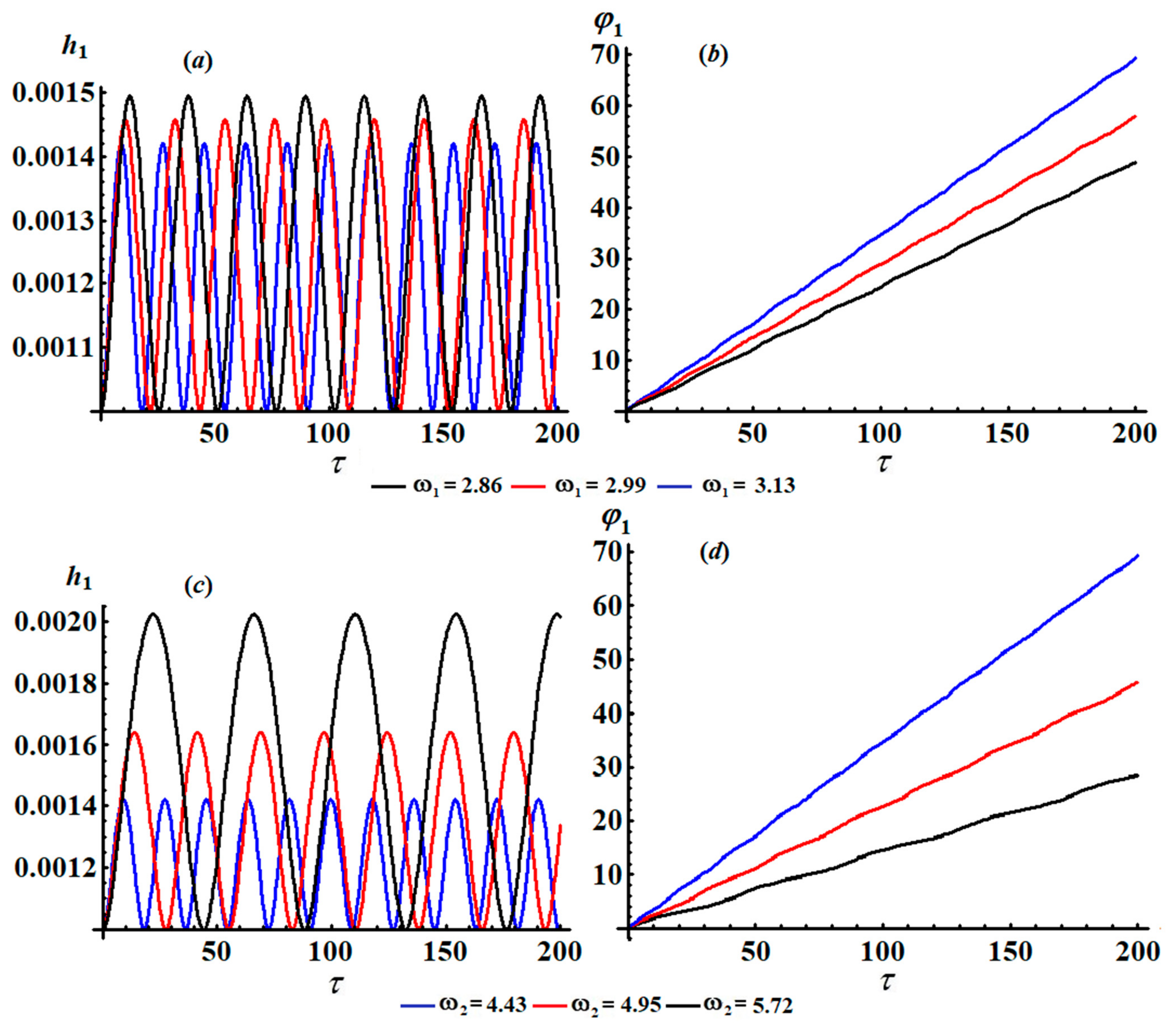
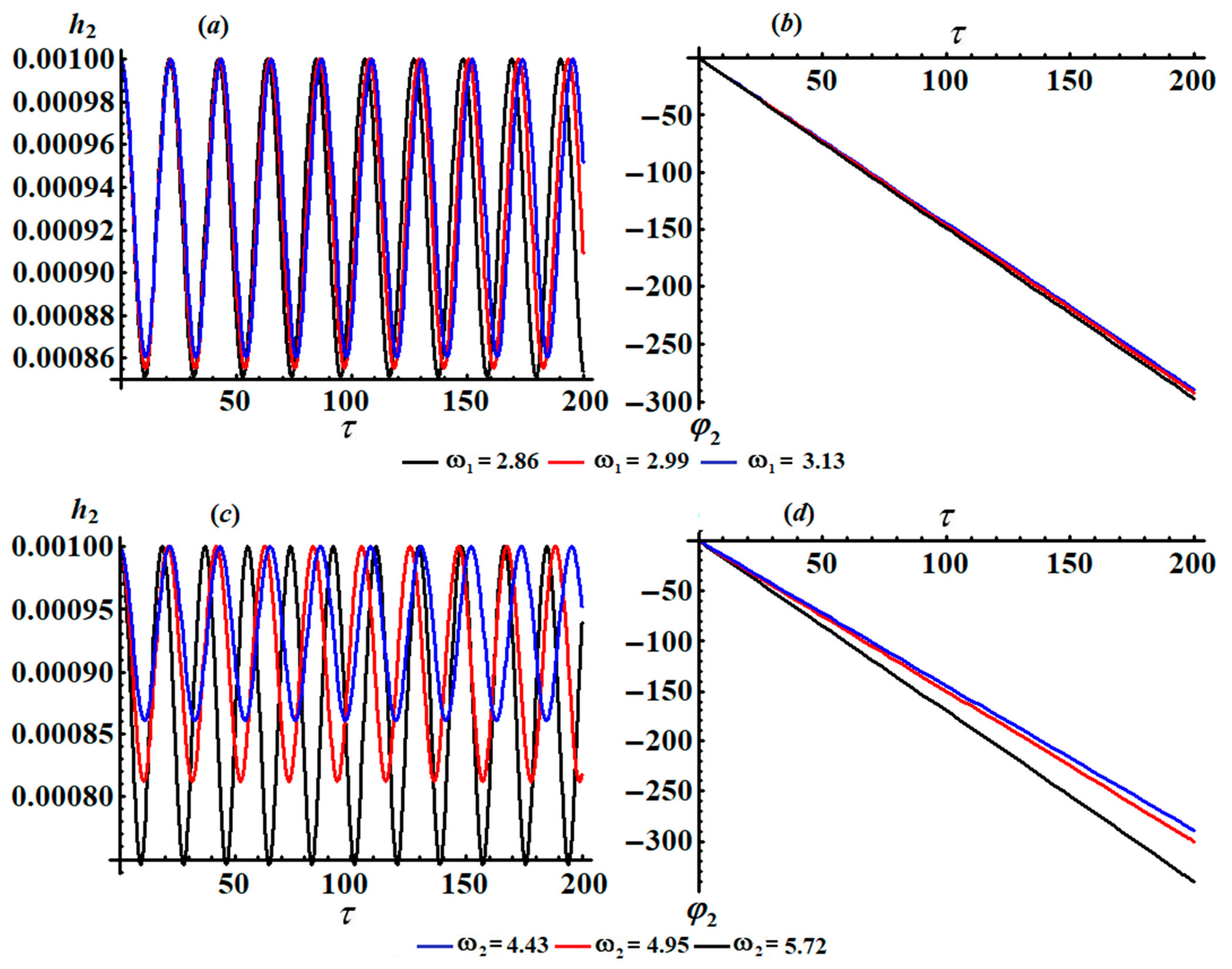
This system is known by the system of modulation equations that consists of four first order ODEs in terms of amplitudes $h_1,h_2$ and modified phases ${\phi }_1,\hspace{0.17em}{\phi }_2$. The equations can be solved based on the initial conditions after transformation to new variables. The attained solutions are drawn in Figure 2 and Figure 3 for different values of ${\omega }_1$ and ${\omega }_2$, in which the following parameters are used:

$${\sigma }_1=-0.01,\hspace{0.17em}\hspace{0.17em}{\sigma }_2=-0.02,\hspace{0.17em}\hspace{0.17em}{f}_1=0.0002,\hspace{0.17em}{f}_2=0.0003,\hspace{0.17em}{p}_1=1+{\sigma }_1,\hspace{0.17em}{p}_2=\omega +{\sigma }_2.\hspace{0.17em}$$

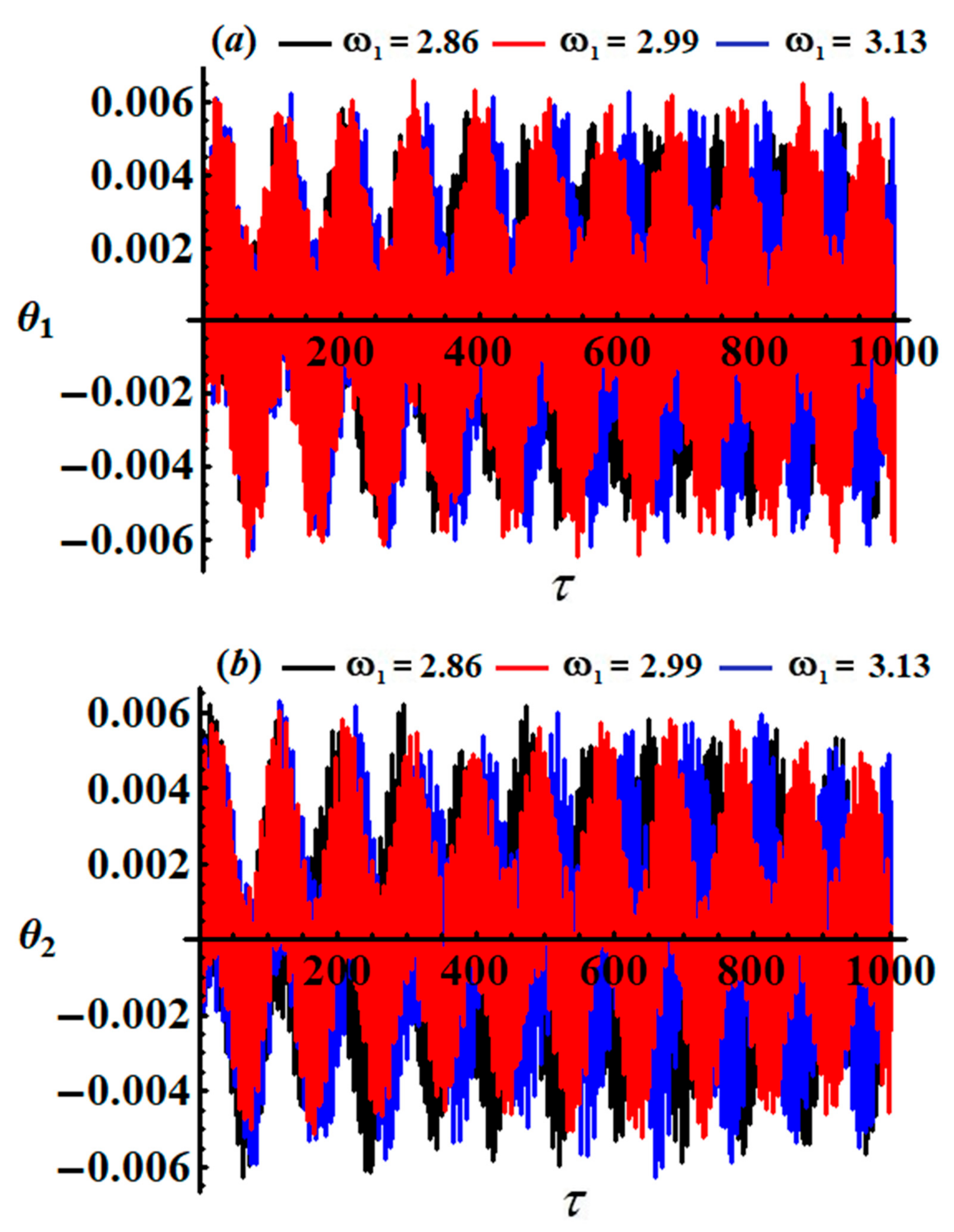
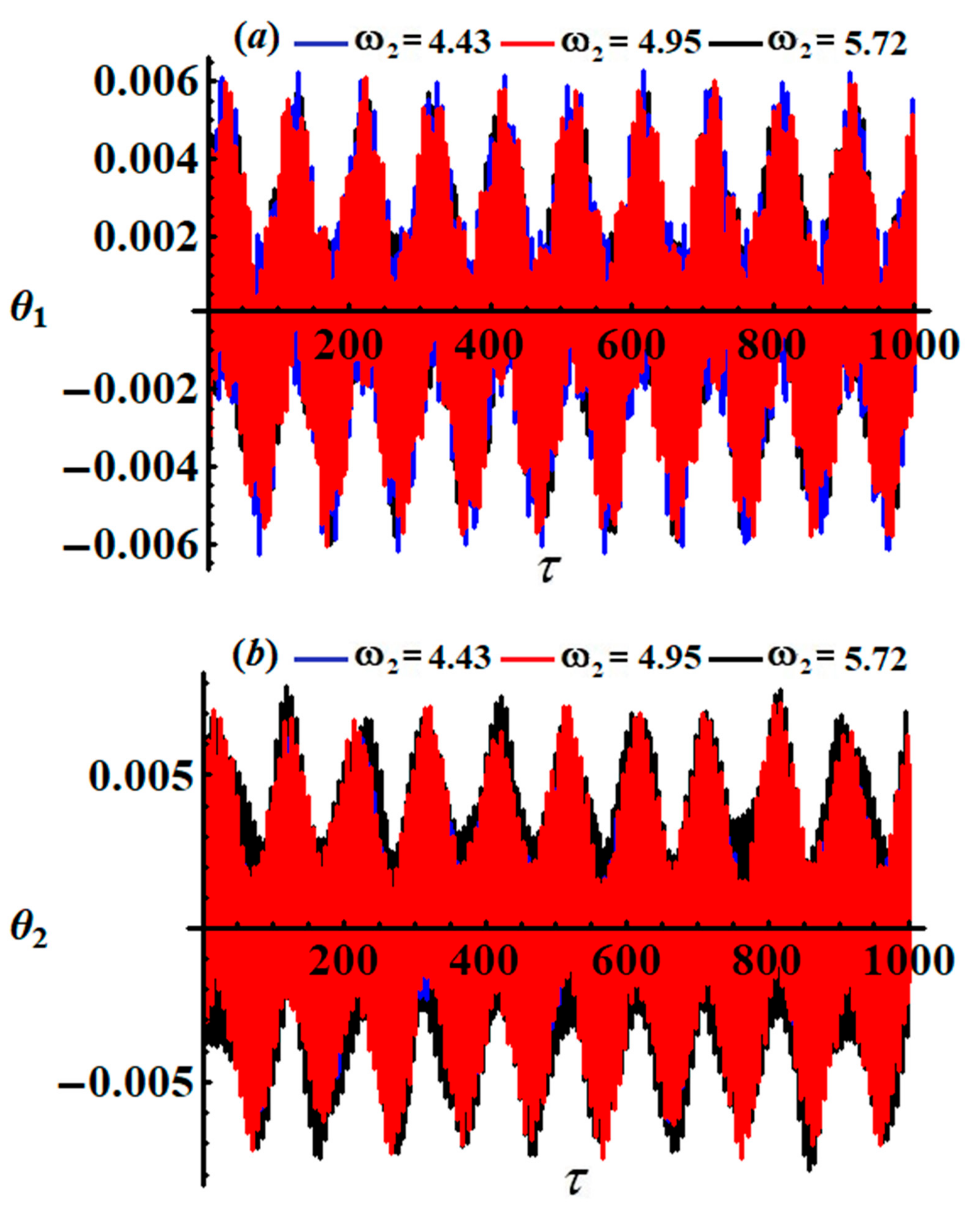
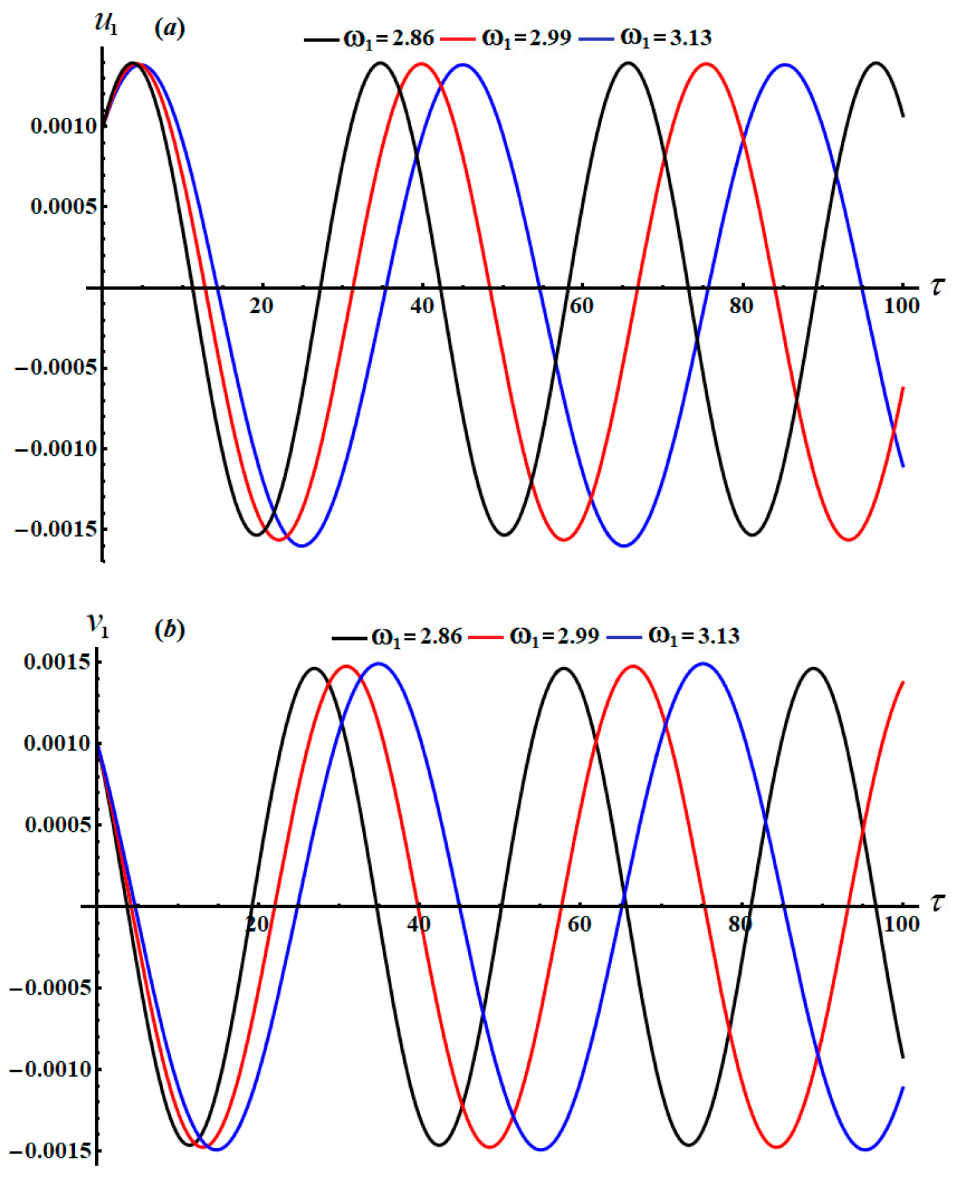
Figure 4 and Figure 5 show the variation of the approximate solutions (AS) ${\theta }_1$ and ${\theta }_2$ up to the third order of approximation with the time parameter $\tau$ for different values of ${\omega }_1$ and ${\omega }_2$, taking into account the previous data. The drawn curves in these figures clarify quasiperiodic waves for the angle ${\theta }_1$ as seen in parts (a) of Figure 4 and Figure 5, while parts (b) of the same figures show the quasiperiodic waves that describe the behavior of angle ${\theta }_2$. The reason for quasi periodicity is owing to the influence of the nonlinearity of the system’s parameters.

An inspection of the curves of Figure 5 shows that the amplitudes of angle ${\theta }_1$ decrease with an increasing ${\omega }_2$ as seen in Figure 5a. However, the amplitudes of angle ${\theta }_2$ increase with the increase in ${\omega }_2$ values, as indicated in Figure 5b.

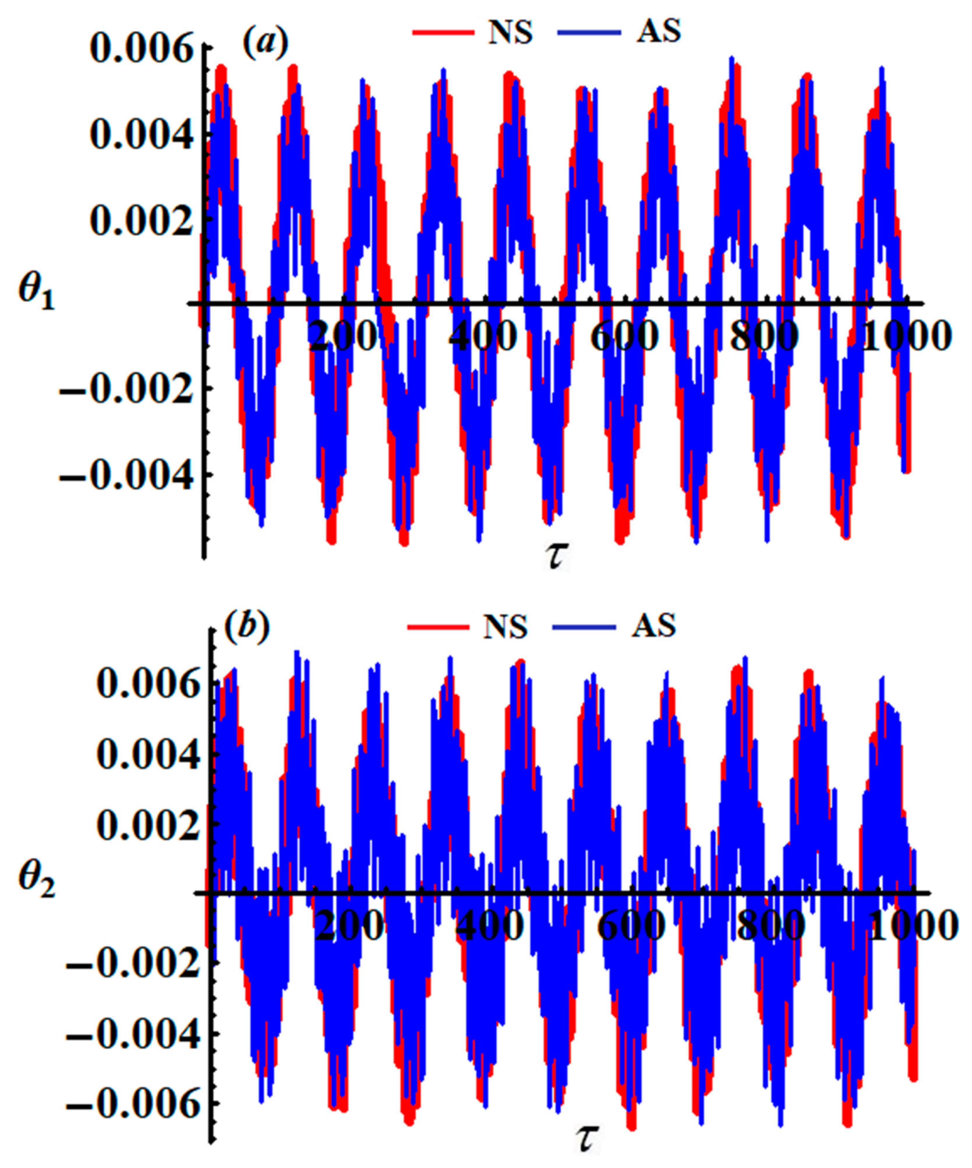
The numerical solutions (NS) of the controlling system of motion are examined using the fourth order Runge–Kutta method in accordance with the above data besides the values of the frequencies, ${\omega }_1=3.3$ and ${\omega }_2=4.4$, and the initial values, ${\theta }_1(0)=0.0002$ and ${\theta }_2(0)=0.0015$. Looking closely at the curves of Figure 6, we conclude that there is an excellent match between the analytical and numerical solutions in the comparison between them, suggesting high accuracy of the MST.

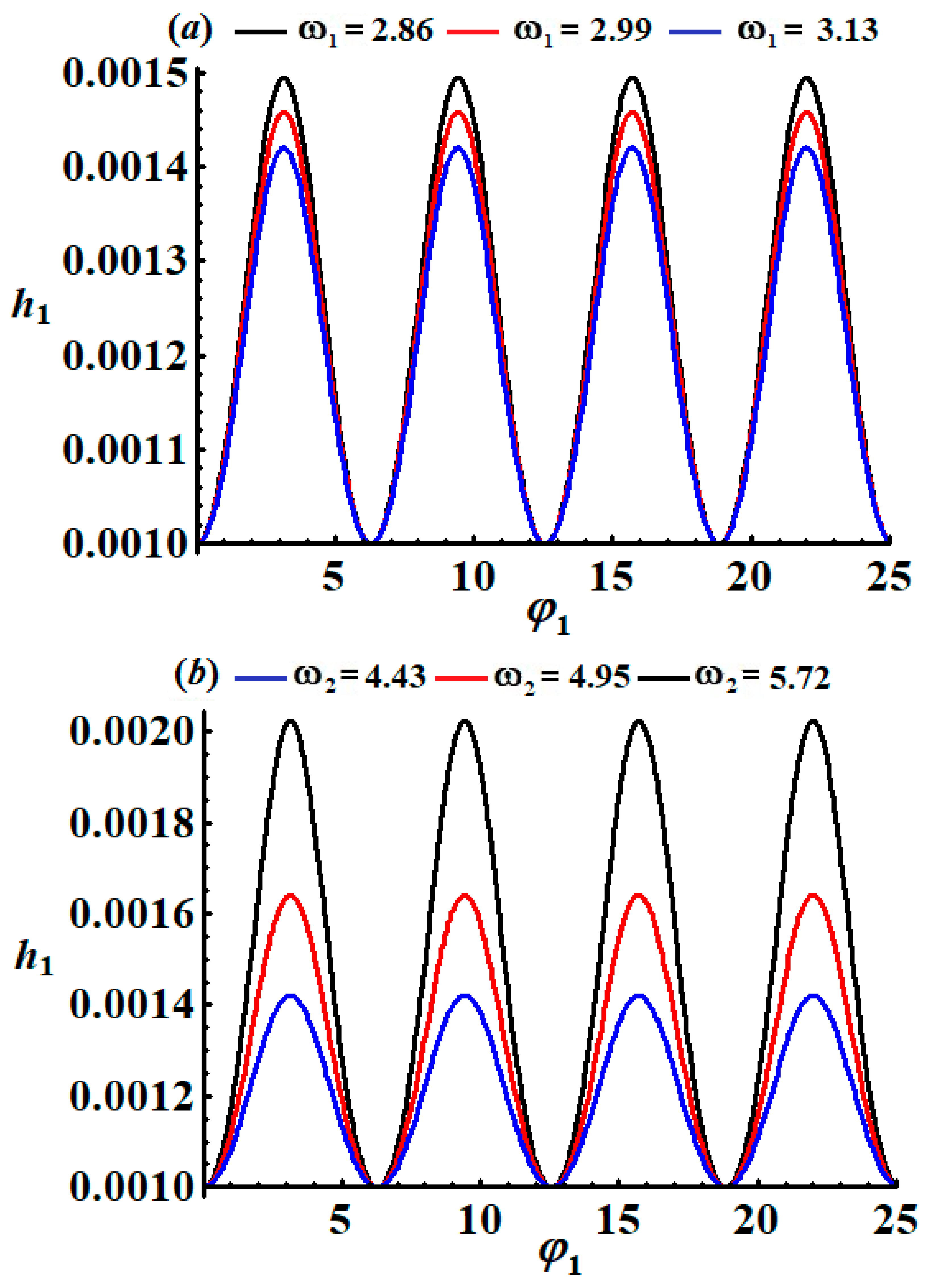
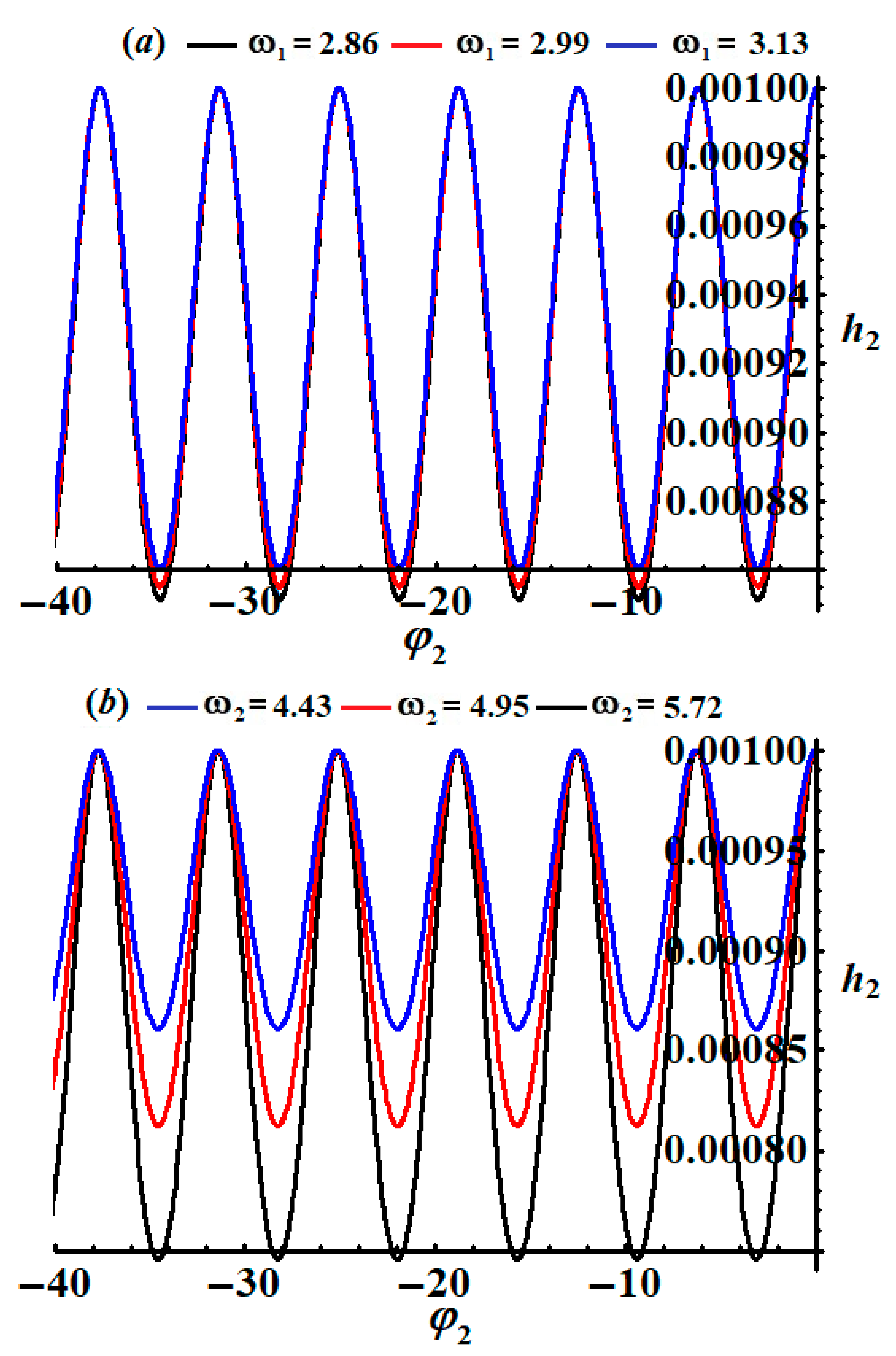
When we follow fluctuations of the studied dynamic system; Equation (37) allows us to see whether they are steady or not. The drawn trajectories of the amplitudes and the adjusted phases are thought to be the best way to characterize the behaviour of the system. A closer look at the curves of Figure 7 and Figure 8 shows periodic waves are observed with various amplitudes when ${\omega }_1$ and ${\omega }_2$ have different values, where the amplitudes of waves decrease with the increase in ${\omega }_1$ and ${\omega }_2$.

5. Steady-State Case

The major goal of this section is to investigate the oscillations of the studied model at the steady state. The modified phases and amplitudes at the steady state can be gained from Equation (37) when the value of the derivatives of their left-hand side is zero, i.e., $(\frac{d{\phi }_j}{dt}=\frac{d{h}_j}{dt}=0;j=1,2)$ [26]. Therefore, one obtains the following algebraic system of the four equations in terms of $h_j$ and ${\phi }_j\hspace{0.17em}\hspace{0.17em}(j=1,2)$:

$$\begin{array}{l}{h}_1{\sigma }_1+\frac{\mu {\omega }^2{h}_1}{2({\omega }^2-1)}+\frac{h_1^3}{16}+\frac{f_1}{2}\cos {\phi }_1=0,\\ \frac{f_1}{2}\sin {\phi }_1=0,\\ h_2{\sigma }_2+\frac{\mu {\omega }^6{h}_2}{2(1-{\omega }^2)}+\frac{{\omega }^2{h}_2^3}{16}+\frac{f_2}{2}\cos {\phi }_2=0,\\ \frac{f_2}{2\omega }\sin {\phi }_2=0.\end{array}$$

(38)

Removing the modified phases ${\phi }_1$ and ${\phi }_2$ from (38), yields the following two algebraic equations regarding the amplitudes $h_j$ and the frequency clarified by the detuning parameters ${\sigma }_j$:

$$\begin{array}{l}{f}_1{}^2=4{(h_1{\sigma }_1+\frac{\mu {\omega }^2{h}_1}{2({\omega }^2-1)}+\frac{h_1^3}{16})}^2,\\ f_2{}^2=4{(h_2{\sigma }_2+\frac{\mu {\omega }^6{h}_2}{2(1-{\omega }^2)}+\frac{{\omega }^2{h}_2^3}{16})}^2.\end{array}$$

(39)

To investigate the stability near fixed points and to examine the stability of the particular steady-state solutions, we consider

$$\begin{array}{l}{h}_1=h_{10}+h_{11},\hspace{0.17em}\hspace{0.17em}\hspace{0.17em}\hspace{0.17em}\hspace{0.17em}\hspace{0.17em}\hspace{0.17em}\hspace{0.17em}\hspace{0.17em}\hspace{0.17em}\hspace{0.17em}\hspace{0.17em}\hspace{0.17em}{h}_2=h_{20}+h_{21},\\ {\phi }_1={\phi }_{10}+{\phi }_{11},\hspace{0.17em}\hspace{0.17em}\hspace{0.17em}\hspace{0.17em}\hspace{0.17em}\hspace{0.17em}\hspace{0.17em}\hspace{0.17em}\hspace{0.17em}\hspace{0.17em}\hspace{0.17em}{\phi }_2={\phi }_{20}+{\phi }_{21},\end{array}$$

(40)

where $h_{10},h_{20},{\phi }_{10},$ and ${\phi }_{20}$ represent the steady-state solutions of Equation (37), while $h_{11},h_{21},{\phi }_{11},$ and ${\phi }_{21}$ denote the perturbations that are supposed to be smaller.

By substituting (40) into (37), we can obtain the linearized equations in the following forms:

$$\begin{array}{l}{h}_{10}\frac{d{\phi }_{11}}{d\tau }=h_{11}{\sigma }_1+\frac{\mu {\omega }^2{h}_{11}}{2({\omega }^2-1)}+\frac{3}{16}{h}_{11}{h}_{10}^2-\frac{f_1}{2}{\phi }_{11}\sin {\phi }_{10},\\ \frac{d{h}_{11}}{d\tau }=\frac{f_1}{2}{\phi }_{11}\cos {\phi }_{10},\\ h_{20}\frac{d{\phi }_{21}}{d\tau }=h_{21}{\sigma }_2+\frac{\mu {\omega }^6{h}_{21}}{2(1-{\omega }^2)}+\frac{3{\omega }^2}{16}{h}_{21}{h}_{20}^2-\frac{f_2}{2}{\phi }_{21}\sin {\phi }_{20},\hspace{0.17em}\hspace{0.17em}\hspace{0.17em}\hspace{0.17em}\hspace{0.17em}\hspace{0.17em}\hspace{0.17em}\hspace{0.17em}\hspace{0.17em}\hspace{0.17em}\hspace{0.17em}\hspace{0.17em}\\ \frac{d{h}_{21}}{d\tau }=\frac{f_2}{2\omega }{\phi }_{21}\cos {\phi }_{20}.\end{array}$$

(41)

Note that small perturbations $h_{11},h_{21},{\phi }_{11},$ and ${\phi }_{21}$ are unknown functions. Each solution can be regarded as a linear combination of $c_s\hspace{0.17em}{e}^{\lambda \tau }$, in which $c_s\hspace{0.17em}\hspace{0.17em}(s=1,2,3,4)$ are constants and $\lambda$ is their corresponding eigenvalue that can be obtained from the roots’ real parts. If the solutions $h_{10},h_{20},{\phi }_{10},$ and ${\phi }_{20}$ at the steady state are asymptotically stable, the roots of real parts of the following characteristic equation must be negative [25]:

$${\lambda }^4+{\Gamma }_1{\lambda }^3+{\Gamma }_2{\lambda }^2+{\Gamma }_3\lambda +{\Gamma }_4=0,$$

(42)

where ${\Gamma }_s\hspace{0.17em}\hspace{0.17em}(s=1,2,3,4)$ are given in terms of $h_{10},h_{20},{\phi }_{10},{\phi }_{20},f_1,$ and $f_2$, in which they have the following forms:

$$\begin{array}{cc}\hfill {\Gamma }_1& =\frac{1}{2}(\frac{f_1\sin {\phi }_{10}}{h_{10}}+\frac{f_2\sin {\phi }_{20}}{h_{20}}),\hfill \\ \hfill {\Gamma }_2& =\{\omega f_1[8({\omega }^2-1)\sin {\phi }_{10}\sin {\phi }_{20}{f}_2+\cos {\phi }_{10}{h}_{20}(-3({\omega }^2-1)h_{10}^2\hfill \\ & -8[\mu {\omega }^2+2({\omega }^2-1){\sigma }_1]))+\cos {\phi }_{20}{f}_2{h}_{10}(-3{\omega }^2({\omega }^2-1)h_{20}^2\hfill \\ & +8(\mu {\omega }^6-2({\omega }^2-1){\sigma }_2)]\}/\{32\omega ({\omega }^2-1)h_{10}{h}_{20}\},\hfill \\ \hfill {\Gamma }_3& =\{f_1{f}_2[-3\omega ({\omega }^2-1)\cos {\phi }_{10}\sin {\phi }_{20}{h}_{10}^2-3{\omega }^2({\omega }^2-1)\cos {\phi }_{20}\hfill \\ & \times \sin {\phi }_{10}{h}_{20}^2-8[\omega ({\omega }^3\cos {\phi }_{20}\sin {\phi }_{10}-\cos {\phi }_{10}\sin {\phi }_{20})\mu {\omega }^2\hfill \\ & -2({\omega }^2-1)(\omega \cos {\phi }_{10}\sin {\phi }_{20}{\sigma }_1+\cos {\phi }_{20}\sin {\phi }_{10}{\sigma }_2)]]\}/(64\omega ({\omega }^2-1)h_{10}{h}_{20}),\hfill \\ \hfill {\Gamma }_4& =\{\cos {\phi }_{10}\cos {\phi }_{20}{f}_1{f}_2[3({\omega }^2-1)h_{10}^2+8(\mu {\omega }^2+2({\omega }^2-1){\sigma }_1)]\hfill \\ & \times [3{\omega }^2({\omega }^2-1)h_{20}^2-8(\mu {\omega }^6-2({\omega }^2-1){\sigma }_2)]\}/[1024\omega ({\omega }^2-1)h_{10}{h}_{20}].\hfill \end{array}$$

(43)

Based on the Routh–Hurwitz criterion [27] and the following determinant:

$$De{t}_{\mathrm{k}}\left[\left(\begin{array}{cccccc}{\Gamma }_1& 1& 0& 0& \dots & 0\\ {\Gamma }_3& {\Gamma }_2& {\Gamma }_1& 1& \dots & 0\\ {\Gamma }_5& {\Gamma }_4& {\Gamma }_3& {\Gamma }_2& \dots & 0\\ {\Gamma }_7& {\Gamma }_6& {\Gamma }_5& {\Gamma }_4& \dots & 0\\ :& :& :& :& :& :\\ {\Gamma }_{2\mathrm{k}-1}& {\Gamma }_{2\mathrm{k}-2}& {\Gamma }_{2\mathrm{k}-3}& \dots & \dots & {\Gamma }_{\mathrm{k}}\end{array}\right)\right]\hspace{0.17em},$$

we can write the stability conditions at the steady-state solutions in the following forms:

$$\begin{array}{cc}{\Gamma }_1>0,\hfill & {\Gamma }_3({\Gamma }_1{\Gamma }_2-{\Gamma }_3)-{\Gamma }_4{\Gamma }_1{}^2>0,\hfill \\ {\Gamma }_1{\Gamma }_2-{\Gamma }_3>0,\hfill & {\Gamma }_4>0.\hfill \end{array}$$

(44)

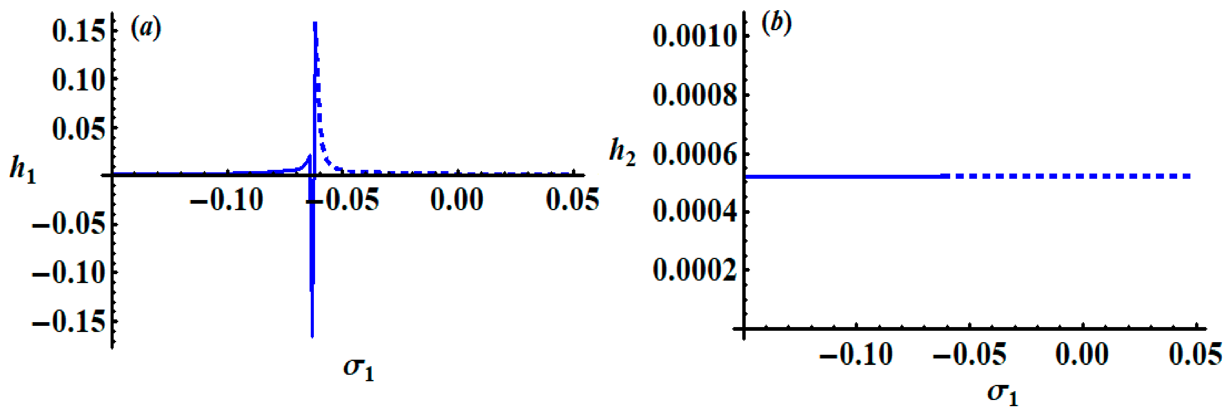
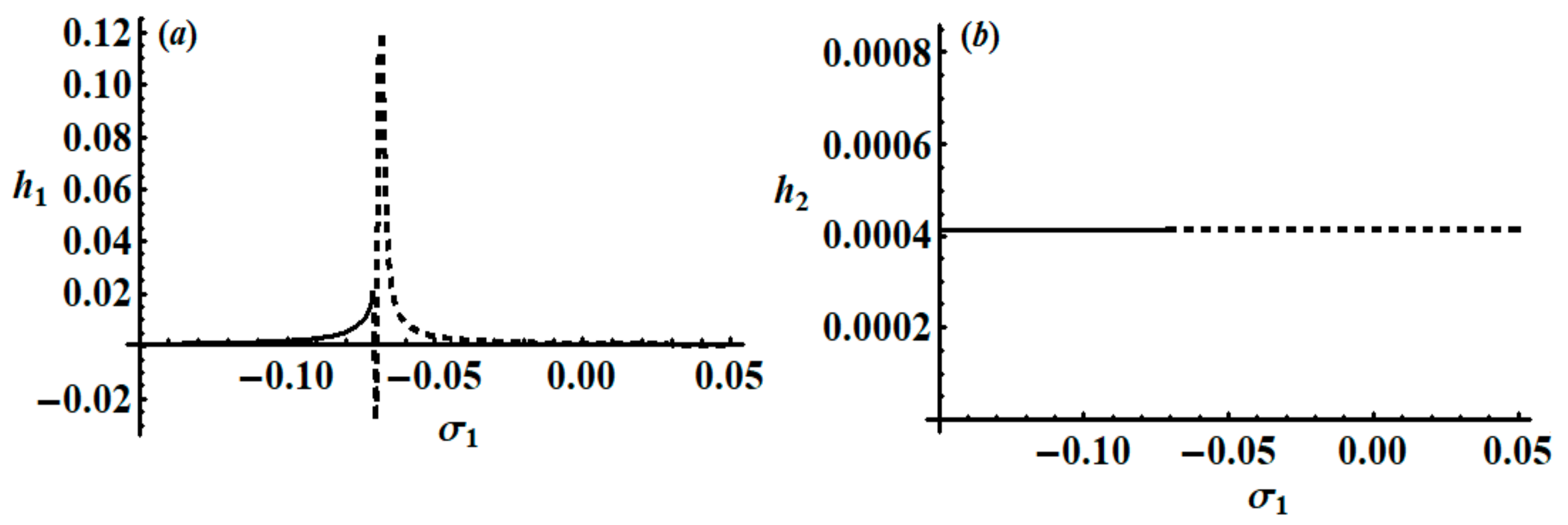
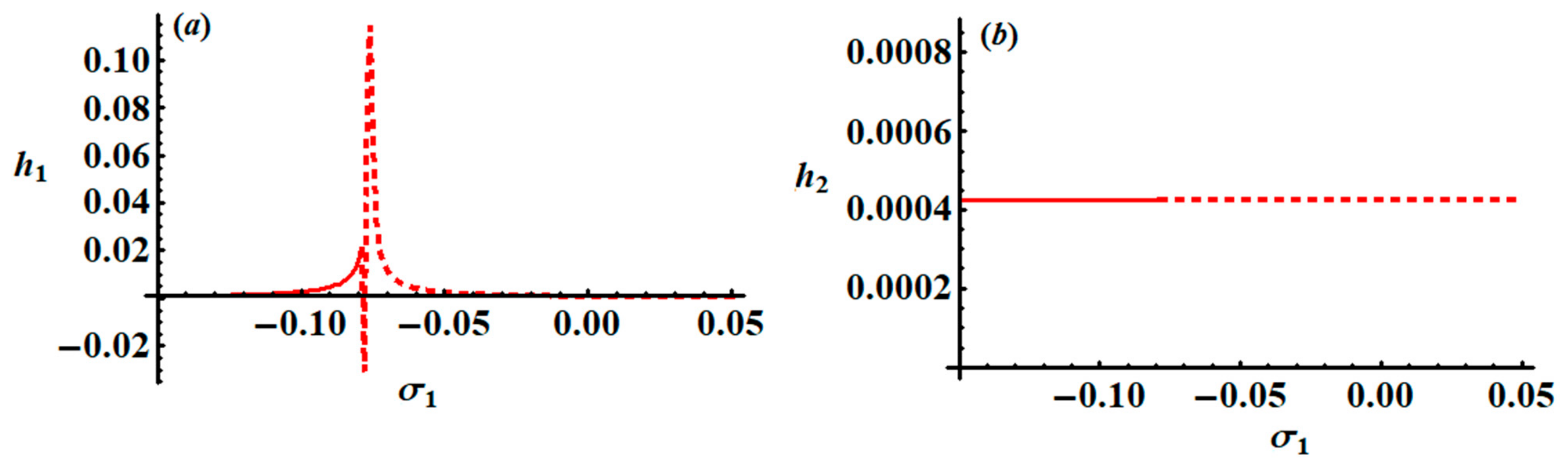
Some of the resonance curves are graphed in Figure 9, Figure 10 and Figure 11, keeping in mind the following parameter data: $f_1=0.0002,\hspace{0.17em}\hspace{0.17em}{f}_2=0.0003,\hspace{0.17em}\hspace{0.17em}\omega =1.414,$ and $\mu =0.32.$ In Figure 9 and Figure 10, modulation amplitudes are plotted versus the detuning parameter ${\sigma }_1$; we investigate that in the region $-0.15\le {\sigma }_1<0.05$ at $\hspace{0.17em}{\sigma }_2=-0.005\hspace{0.17em},$ there exists one possible critical fixed point. This point is stable in the region $-0.15\le {\sigma }_1\le -0.062$ but it loses its stability for $-0.062<{\sigma }_1\le 0.05$, as indicated in Figure 9. On the other hand, the stable fixed points are found in the region $-0.15\le {\sigma }_1\le -0.071$ at $\hspace{0.17em}{\sigma }_2=-0.05\hspace{0.17em}$, while it will be unstable in the area $-0.071<{\sigma }_1\le 0.05$, as seen in Figure 10. Moreover, Figure 11 shows the modulation amplitudes versus the detuning parameter ${\sigma }_1$ in the region $-0.15\le {\sigma }_1<0.05$ at $\hspace{0.17em}{\sigma }_2=0,$ where only one possible critical point exists. The fixed point is stable in the region $-0.15<{\sigma }_1\le -0.079$ but it is unstable in the region $-0.079<{\sigma }_1<0.05$.

6. Non-Linear Analysis

In this section, we will demonstrate the properties of nonlinear amplitude for the system of Equations (37) and investigate their stabilities [28,29,30]. Then, the transformations below are taken into account

$$A_j=[U_j({\tau }_2)+i{V}_j({\tau }_2)]\hspace{0.17em}{e}^{i{\tilde{\sigma }}_j{\tau }_1};\hspace{0.17em}\hspace{0.17em}\hspace{0.17em}\hspace{0.17em}\hspace{0.17em}(j=1,2)$$

(45)

where

$$U_j=\epsilon \hspace{0.17em}{u}_j,\hspace{0.17em}\hspace{0.17em}\hspace{0.17em}\hspace{0.17em}\hspace{0.17em}\hspace{0.17em}\hspace{0.17em}\hspace{0.17em}{V}_j=\epsilon \hspace{0.17em}{v}_j;\hspace{0.17em}\hspace{0.17em}\hspace{0.17em}\hspace{0.17em}\hspace{0.17em}(j=1,2).$$

Making use of (11) and (45) in (37), and separating the real parts and the imaginary ones yields the next system, which is as follows:

$$\begin{array}{l}\frac{d{u}_1}{d\tau }=v_1\{{\sigma }_1+\frac{\mu {\omega }^2}{2({\omega }^2-1)}+\frac{1}{4}(u_1^2+v_1^2)\},\\ \frac{d{v}_1}{d\tau }=u_1\{{\sigma }_1-\frac{\mu {\omega }^2}{2({\omega }^2-1)}-\frac{1}{4}(u_1^2+v_1^2)\}-\frac{f_1}{4},\\ \frac{d{u}_2}{d\tau }=v_2\{{\sigma }_2+\frac{\mu {\omega }^5}{2(1-{\omega }^2)}+\frac{1}{4}\omega (u_2^2+v_2^2)\},\\ \frac{d{v}_2}{d\tau }=u_2\{{\sigma }_2-\frac{\mu {\omega }^5}{2(1-{\omega }^2)}-\frac{1}{4}\omega (u_2^2+v_2^2)\}-\frac{f_2}{4\omega }.\end{array}$$

(46)

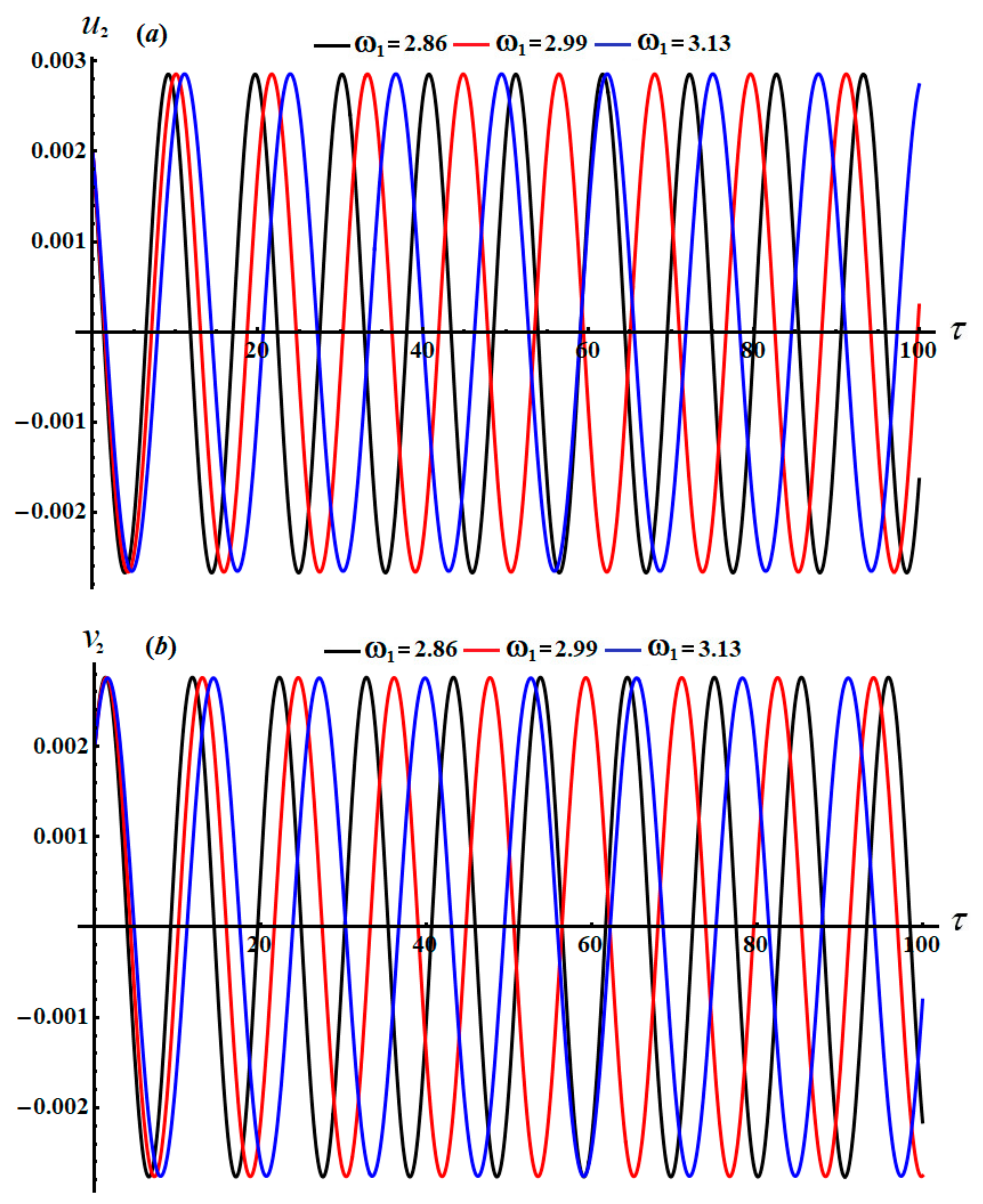
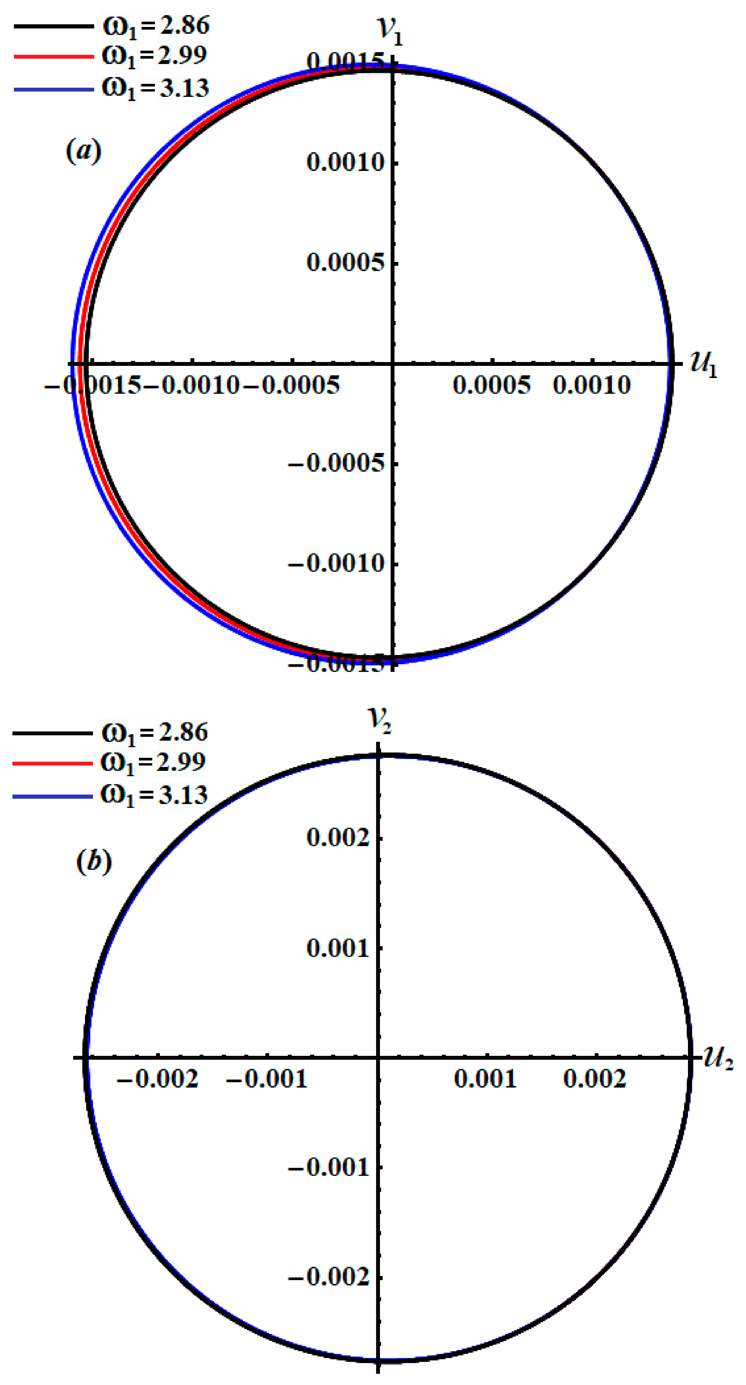
In distinct parametric regions, the altered amplitudes were then analyzed across the used time interval and the attributes of amplitudes were displayed in the curves of the phase plane, as graphed in Figure 12, Figure 13 and Figure 14, taking into account the prior data of the parameters that have been used.

The time histories of $u_j$ and $v_j\hspace{0.17em}\hspace{0.17em}\hspace{0.17em}(j=1,2)$, as specified in system (46), are depicted in Figure 12 and Figure 13. It is appropriate to mention that the drawn curves in these figures have a progressive periodic manner, in which the number of oscillations decreases with the increasing in ${\omega }_1$ values and the wavelength of the waves increases. Moreover, we can predict that the motion of the studied system is stable. Parts (a) and (b) of Figure 14 explore the plots of the phase planes $u_j{v}_j\hspace{0.17em}\hspace{0.17em}(j=1,2)$ in the presence of various values of the frequency ${\omega }_1$. It is observed that symmetric closed curves are portrayed to assert our prediction of the stability and the steady motion of the investigated system.

7. Conclusions

The problem of the nonlinear dynamical motion of a 2-DOF double pendulum with different lengths has been investigated. It has been considered that its pivot point moves in an elliptic trajectory with a steady angular velocity. The governing EOM have been derived utilizing Lagrange’s equations and have been solved up to the third order of approximation using the MST. All the arising resonances cases have been classified. The requirements of solvability of the solutions at the steady state have been obtained. The stability of the possible fixed points has been checked in line with the characteristic Equation (42) and the criterion of Routh–Hurwitz (44). Time histories sketches and resonance curves have been represented graphically. The impact of the various parameters on dynamical motion has been examined using the nonlinear stability approach. The analytical results have been compared with the numerical ones of the governing system of motion to show a high degree of consistency between them, which reflects the great accuracy of the used MST. The importance of the studied model is due to its significant applications in various fields such as physics and engineering applications that are based on vibrating systems such as shipbuilding and ships motion, structure vibration, rotor dynamics, pumps compressors, transportation devices and human or robotic walking analysis.

References

- Strogatz, S.H. Nonlinear Dynamics and Chaos: With Applications to Physics, Biology, Chemistry, and Engineering, 2nd ed.; Princeton University Press: Princeton, NJ, USA, 2015. [Google Scholar]
- Melby, P.; Weber, N.; Hübler, A. Dynamics of self-adjusting systems with noise. Chaos 2005, 15, 33902. [Google Scholar] [CrossRef]
- Jackson, T.; Radunskaya, A. Applications of Dynamical Systems in Biology and Medicine; Springer: New York, NY, USA, 2015. [Google Scholar]
- Dubey, N.H. Engineering Mechanics: Statics and Dynamics; Tata McGraw-Hill Education: New York, NY, USA, 2013. [Google Scholar]
- Kyoung, L.W.; Dong, P.H. Chaotic dynamics of a harmonically excited spring-pendulum system with internal resonance. Nonlinear Dyn. 1197, 14, 211–229. [Google Scholar]
- Lee, W.; Hsu, C. A Global Analysis of an Harmonically Excited Spring-Pendulum System with Internal Resonance. J. Sound Vib. 1994, 171, 335–359. [Google Scholar] [CrossRef]
- Alasty, A.; Shabani, R. Chaotic motions and fractal basin boundaries in spring-pendulum system. Nonlinear Anal. Real World Appl. 2006, 7, 81–95. [Google Scholar] [CrossRef]
- Lee, W.K.; Park, H.D. Second-order approximation for chaotic responses of a harmonically excited spring–pendulum system. Int. J. Non-linear Mech. 1999, 34, 749–757. [Google Scholar] [CrossRef]
- Awrejcewicz, J.; Starosta, R.; Sypniewska-Kamińska, G. Asymptotic Analysis and Limiting Phase Trajectories in the Dynamics of Spring Pendulum; Springer International Publishing: Cham, Switzerland, 2014; pp. 161–173. [Google Scholar]
- Eissa, M.; Kamel, M.; El-Sayed, A.T. Vibration reduction of multi-parametric excited spring pendulum via a transversally tuned absorber. Nonlinear Dyn. 2010, 61, 109–121. [Google Scholar] [CrossRef]
- Awrejcewicz, J.; Starosta, R.; Sypniewska-Kamińska, G. Stationary and Transient Resonant Response of a Spring Pendulum. Procedia IUTAM 2016, 19, 201–208. [Google Scholar] [CrossRef] [Green Version]
- Kamińska, G.S.; Awrejcewicz, J.; Kamiński, H. Resonance study of spring pendulum based on asymptotic solutions with polynomial approximation in quadratic means. Meccanica 2020, 56, 963–980. [Google Scholar] [CrossRef]
- Bek, M.; Amer, T.; Sirwah, M.A.; Awrejcewicz, J.; Arab, A.A. The vibrational motion of a spring pendulum in a fluid flow. Results Phys. 2020, 19, 103465. [Google Scholar] [CrossRef]
- Starosta, R.; Sypniewska-Kaminska, G.; Awrejcewicz, J. Parametric and external resonances in kinematically and externally excited nonlinear spring pendulum. Int. J. Bifurc. Chaos 2011, 21, 3013–3021. [Google Scholar] [CrossRef]
- Amer, T.; Bek, M. Chaotic responses of a harmonically excited spring pendulum moving in circular path. Nonlinear Anal. Real World Appl. 2009, 10, 3196–3202. [Google Scholar] [CrossRef]
- Amer, T.S.; Bek, M.A.; Hamada, I.S. On the Motion of Harmonically Excited Spring Pendulum in Elliptic Path Near Resonances. Adv. Math. Phys. 2016, 2016, 15. [Google Scholar] [CrossRef] [Green Version]
- Amer, T.S.; Bek, M.A.; Abouhmr, M.K. On the vibrational analysis for the motion of a harmonically damped rigid body pendulum. Nonlinear Dyn. 2018, 91, 2485–2502. [Google Scholar] [CrossRef]
- Amer, T.; Bek, M.; Abohamer, M. On the motion of a harmonically excited damped spring pendulum in an elliptic path. Mech. Res. Commun. 2019, 95, 23–34. [Google Scholar] [CrossRef]
- Amer, W.; Bek, M.; Abohamer, M. On the motion of a pendulum attached with tuned absorber near resonances. Results Phys. 2018, 11, 291–301. [Google Scholar] [CrossRef]
- Starosta, R.; Sypniewska-Kaminska, G.; Awrejcewicz, J. Asymptotic analysis of kinematically excited dynamical systems near resonances. Nonlinear Dyn. 2012, 68, 459–469. [Google Scholar] [CrossRef]
- Awrejcewicz, J.; Starosta, R.; Sypniewska-Kamińska, G. Asymptotic Analysis of Resonances in Nonlinear Vibrations of the 3-dof Pendulum. Differ. Equ. Dyn. Syst. 2013, 21, 123–140. [Google Scholar] [CrossRef]
- El-Sabaa, F.M.; Amer, T.S.; Gad, H.M.; Bek, M.A. On the motion of a damped rigid body near resonances under the influence of harmonically external force and moments. Results Phys. 2020, 19, 103352. [Google Scholar] [CrossRef]
- Gupta, M.K.; Sinha, N.; Bansal, K.; Singh, A.K. Natural frequencies of multiple pendulum systems under free condition. Arch. Appl. Mech. 2016, 86, 1049–1061. [Google Scholar] [CrossRef]
- Gupta, M.K.; Sharma, P.; Mondal, A.K.; Kumar, A. Visual Recurrence Analysis of Chaotic and Regular Motion of a Multiple Pendulum System. Arab. J. Sci. Eng. 2017, 42, 2711–2716. [Google Scholar] [CrossRef]
- Amer, T.; Bek, M.; Hassan, S.; Elbendary, S. The stability analysis for the motion of a nonlinear damped vibrating dynamical system with three-degrees-of-freedom. Results Phys. 2021, 28, 104561. [Google Scholar] [CrossRef]
- Nayfeh, A.H. Perturbations Methods; WILEY-VCH Verlag GmbH and Co. KGaA: Weinheim, Germany, 2004. [Google Scholar]
- Gantmacher, F.R. Applications of the Theory of Matrices; John Wiley & Sons: New York, NY, USA, 2005. [Google Scholar]
- Abady, I.; Amer, T.; Gad, H.; Bek, M. The asymptotic analysis and stability of 3DOF non-linear damped rigid body pendulum near resonance. Ain Shams Eng. J. 2021. [Google Scholar] [CrossRef]
- Abohamer, M.K.; Awrejcewicz, J.; Starosta, R.; Amer, T.S.; Bek, M.A. Influence of the Motion of a Spring Pendulum on Energy-Harvesting Devices. Appl. Sci. 2021, 11, 8658. [Google Scholar] [CrossRef]
- He, J.-H.; Amer, T.S.; Elnaggar, S.; Galal, A.A. Periodic Property and Instability of a Rotating Pendulum System. Axioms 2021, 10, 191. [Google Scholar] [CrossRef]
Figure 1.
Description of the model.
Figure 2.
Demonstration of the modulation of the amplitude and modified phase : (a,b) at , (c,d) at .
Figure 3.
Sketches of the modulation of the amplitude and modified phase : (a,b) at , (c,d) at .
Figure 4.
The time histories of the solutions at : (a) for , (b) for .
Figure 5.
Description of the time histories of the solutions at : (a) for , (b) for .
Figure 6.
Representation of a comparison between the AS and the NS at and : (a) for , (b) for .
Figure 7.
Description of the modulation for the amplitude as a function of : (a) at , (b) at .
Figure 8.
Clarification of the modulation of the amplitude as a function of : (a) at , (b) at .
Figure 9.
Sketches of the variation of modulation amplitudes with the detuning parameter at : (a) , (b) .
Figure 10.
Figure 11.
Portrayal of the variation of modulation amplitudes with the detuning parameter at : (a) , (b) .
Figure 12.
Description of the modified amplitudes via when : (a) , (b) .
Figure 13.
Sketches of the modified amplitudes versus when : (a) , (b) .
Figure 14.
Illustration of the projections of the equations of modulation paths when : (a) on the plane , (b) on the plane .
Publisher’s Note: MDPI stays neutral with regard to jurisdictional claims in published maps and institutional affiliations. |
© 2021 by the authors. Licensee MDPI, Basel, Switzerland. This article is an open access article distributed under the terms and conditions of the Creative Commons Attribution (CC BY) license (https://creativecommons.org/licenses/by/4.0/).
Share and Cite
MDPI and ACS Style
Amer, T.S.; Starosta, R.; Elameer, A.S.; Bek, M.A. Analyzing the Stability for the Motion of an Unstretched Double Pendulum near Resonance. Appl. Sci. 2021, 11, 9520. https://doi.org/10.3390/app11209520
AMA Style
Amer TS, Starosta R, Elameer AS, Bek MA. Analyzing the Stability for the Motion of an Unstretched Double Pendulum near Resonance. Applied Sciences. 2021; 11(20):9520. https://doi.org/10.3390/app11209520
Chicago/Turabian StyleAmer, Tarek S., Roman Starosta, Abdelkarim S. Elameer, and Mohamed A. Bek. 2021. "Analyzing the Stability for the Motion of an Unstretched Double Pendulum near Resonance" Applied Sciences 11, no. 20: 9520. https://doi.org/10.3390/app11209520
Note that from the first issue of 2016, this journal uses article numbers instead of page numbers. See further details here.