Accelerated Simulation of Discrete Event Dynamic Systems via a Multi-Fidelity Modeling Framework †


1
Korea Advanced Institute of Science and Technology (KAIST), Daejeon 34141, Korea
2
Daewoo Shipbuilding & Marine Engineering (DSME), Seoul 04521, Korea
*
Author to whom correspondence should be addressed.
†
This paper is an extension of the conference paper, “Multi-Fidelity Modeling & Simulation Methodology for Simulation Speed Up,” presented in the 2nd ACM SIGSIM Conference on Principles of Advanced Discrete Simulation, Denver, CO, USA, 18–21 May 2014.
Appl. Sci. 2017, 7(10), 1056; https://doi.org/10.3390/app7101056
Submission received: 7 September 2017
/
Revised: 4 October 2017
/
Accepted: 12 October 2017
/
Published: 13 October 2017
(This article belongs to the Special Issue Modeling, Simulation, Operation and Control of Discrete Event Systems)
Abstract
:Simulation analysis has been performed for simulation experiments of all possible input combinations as a “what-if” analysis, which causes the simulation to be extremely time-consuming. To resolve this problem, this paper proposes a multi-fidelity modeling framework for enhancing simulation speed while minimizing simulation accuracy loss. A target system for this framework is a discrete event dynamic system. The dynamic property of the system facilitates the development of variable fidelity models for the target system due to its high computational cost; and the discrete event property allows for determining when to change the fidelity within a simulation scenario. For formal representation, the paper defines several key concepts such as an interest region, a fidelity change condition, and a selection model. These concepts are integrated into the framework to allow for the achievement of a condition-based disjunction of high- and low-fidelity simulations within a scenario. The proposed framework is applied to two case studies: unmanned underwater and urban transportation vehicles. The results show that simulation speed increases at least 1.21 times with a 5% accuracy loss. We expect that the proposed framework will resolve a computationally expensive problem in the simulation analysis of discrete event dynamic systems.
1. Introduction
Simulation analysis is playing an increasingly prominent role in resolving real-world problems that cannot be solved with numerical and analytical methods [1]. For example, in the system-on-chip field, distributed cosimulation is a practical approach to unify and analyze abstracted hardware resources [2]. In the social systems, simulations have been utilized to evaluate passenger flow organization and facility layout at metro stations [3] or to find an optimal condition for the growth of crops in greenhouse control systems [4]. Generally, such a simulation analysis requires one to perform simulation evaluations of all possible input combinations as a ‘‘what-if’’ analysis [5]; thus, it consumes too much simulation execution time due to many repeated experiments. To reduce the execution time, various studies have been conducted: the distributed execution of simulators using hardware resources [6], parallel event scheduling using the graphics processing units [7], a flattening simulation algorithm for hierarchical models [8], and simulation-based optimization integrating a meta-model and a meta-heuristic method [9], etc.
This paper focuses on a multi-fidelity modeling scheme to achieve simulation speedup for simulation analysis. In the simulation world, the most common use of the term “fidelity” refers to the faithfulness with which model behavior reflects modeled system behavior [10,11]. For the models that represent the same reference system, fidelity is compared by their outputs for the same input. In other words, a high-fidelity model has a high accuracy in model output compared to the reference system, whereas a low-fidelity model has a relatively less accurate output. Because the high-fidelity simulation is very time-consuming due to the high computational load, an appropriate portion of a simulation scenario requires simulating with high-fidelity models.
To decrease the simulation time without significant loss in respect to simulation accuracy, we propose a multi-fidelity modeling framework. The proposed framework consists of a dynamical conversion process between high- and lower-fidelity models. It employs a fidelity change approach to select a suitable model from a pool of models with variable fidelities. Within a single simulation scenario (i.e., a simulation design point), all the time frames need not be simulated with high-fidelity models [12]. Therefore, the high-fidelity models are primarily used for important regions of the scenario, whereas the lower-fidelity models are used for marginal parts. In this context, the point of our framework is to decide which model needs to change its level of fidelity and to know when to change the fidelity within the simulation scenario.
To this end, we define three concepts in the framework: (1) an interest region where the model output has a serious effect on the overall simulation analysis, (2) a fidelity change condition (FCC) to check whether the fidelity of the model needs to be changed based on the defined interest region, and (3) a selection model to choose a model with the proper fidelity when the FCC is satisfied. The proposed framework, based on these concepts, allows the achievement of a condition-based transformation between high- and low-fidelity simulations within a scenario, reducing the overall computational cost and ensuring the accuracy of the simulation analysis.
The targeted system of this paper is a discrete event dynamic system. It exhibits hybrid behaviors characterized by a set of continuous laws that are switched by discrete events [13]. The dynamic property facilitates the development of apparent high- and low-fidelity models for a target system, and the discrete event property allows one to know when the level of fidelity is changed with discrete events. In our framework, these concepts are proposed with formal modeling specifications. In particular, this paper uses the discrete time system specification (DTSS) for the dynamic system model and the discrete event system specification (DEVS) for the discrete event system [14]. Such a formal modeling approach facilitates maximizing the reusability of existing models and simulation algorithms.
In recent years, multi-fidelity modeling and simulation (M&S) have been studied in many application fields such as aerospace engineering [15], submarine systems [16], computational fluid dynamics [17], and supply chain systems [18], etc. A common point of these studies is to drive the preliminary design process using low-fidelity models as surrogates for expensive high-fidelity simulations. High-fidelity models are then used in the final design stages to refine the design. This means that the fidelity change has not occurred during the same simulation scenario. In addition, these studies focused on application-oriented methods, which have key differences from our study.
For experimentation, we performed two practical applications that show the effectiveness of the proposed framework in simulation speedup and accuracy. An unmanned underwater vehicle (UUV) was modeled for the dynamic system, and urban transportation vehicles (UTVs) were modeled for the discrete event system. For empirical evaluations, we define two measurements (i.e., an output error and a speedup ratio). The proposed modeling framework enhances the simulation speed about 1.25 times and 1.21 times for each application with an accuracy loss of about 5%. Additionally, due to the use of formal representation, most existing models and simulation engines were reused without any modifications.
This paper is organized as follows. Section 2 explains the target system, model fidelity, and simulation region, and Section 3 introduces the literature review. Section 4 describes the proposed multi-fidelity modeling framework. The two case studies are described in Section 5, and a conclusion is given in Section 6.
2. Problem Definition
2.1. Target System
A discrete event dynamic system is a (typically asynchronous) dynamic system in which state transitions are triggered by the occurrence of discrete events [19]. In the following subsections, we introduce the target system by distinguishing between two systems: dynamic and discrete event systems.
2.1.1. Dynamic System
The output (Y(t)) of a dynamic system is affected by the inputs (X(τ)) for τ ≤ t; in other words, not only the input at the present time (u(t)) but also its past inputs (u(τ)) will affect the system (for τ < t) [20]. For a simulation of the dynamic system, simulation time is divided into many small steps (i.e., discrete time tick). The system model evolves its states at each time step, assuming that the states are unchanged during a time step. This is a typical characteristic of discrete time simulations; thus, the discrete time system models are usually the most intuitive to grasp all forms of the dynamic system models [18].
The dynamic system using a discrete time simulation has numerous applications. For example, a compartment dynamic model was simulated to describe the dynamic response and distribution characteristics of the gasifier [21], and trajectories of unmanned aerial vehicles were modeled for collision avoidance [22]. In this paper, the maneuvering behaviors of a UUV are modeled based on the DTSS, which is a generalized form of a Mealy system [18].
Figure 1 shows the structure of a DTSS model and the following specification is its formal representation [23]. The DTSS model consists of three variable sets (i.e., input, output, and state sets) and two functions—state transition and output functions. Input, output, and state variables have continuous values according to the simulation time. The state transition function, f(t), updates the state at the next time instant given the current state and input values. Note that a derivative equation is used to specify the rate of change of the state variables for the state transition function. The output function, g(t), also requires state and input variables. At any particular time instant on the time axis, given the current state and input values, the function computes the output values. In the DTSS model of Figure 1, the state variable is represented by a circle and the two functions are depicted with squares.
- is the set of inputs;
- is the set of outputs;
- is the set of continuous states;
- is the state transition function;
- is the output function.
2.1.2. Discrete Event System
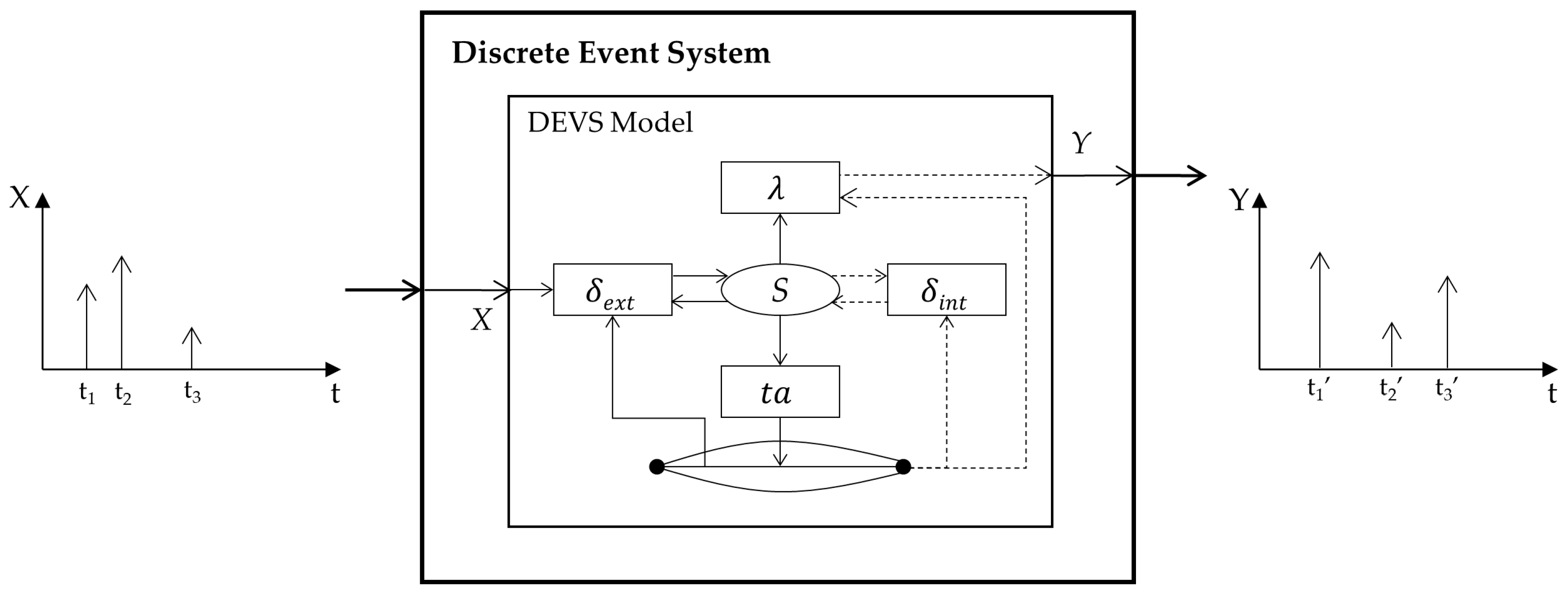
A discrete event system is an event-driven system in which discrete states are updated depending entirely on the occurrence of asynchronous discrete events over time. In discrete event simulations, system states are scheduled dynamically as the simulation proceeds. Various modeling schemes (e.g., finite state machine, Petri-net, DEVS, or Markov chain) have been used for discrete event simulations [24,25,26,27,28]. Among them, the DEVS is a modular and hierarchical formalism for object-oriented modeling and analysis [2], which is our approach for modeling the discrete event system.
Figure 2 shows the structure of a DEVS atomic model and the following specification is its formal representation [18]. The DEVS atomic model consists of three variables and four functions. As the DTSS model in Figure 1, a circle in the DEVS model represents the state variable and the squares indicate the functions. System behaviors in the model are represented by state transitions using input and output events. State variables with discrete values are updated by two transitions: when the model receives an input event, state variables are updated; otherwise, if it does not receive any input events until a certain time, an output event occurs and the state variables are renewed. The former case is conducted by an external transition function, and the latter one is carried out by an output and an internal transition function. The amount of time that a state waits for an input event is decided by a time advance function. In Figure 2, the solid arrows in the DEVS model are relevant to the former case, whereas the dotted ones correlate to the latter case. We modeled UTVs with the DEVS formalism, which will be explained in Section 5.
- is the set of inputs;
- is the set of outputs;
- is the set of states;
- is the external transition function
- ;
- is the internal transition function;
- is the output function;
- is the time advance function.
2.2. Model Fidelity
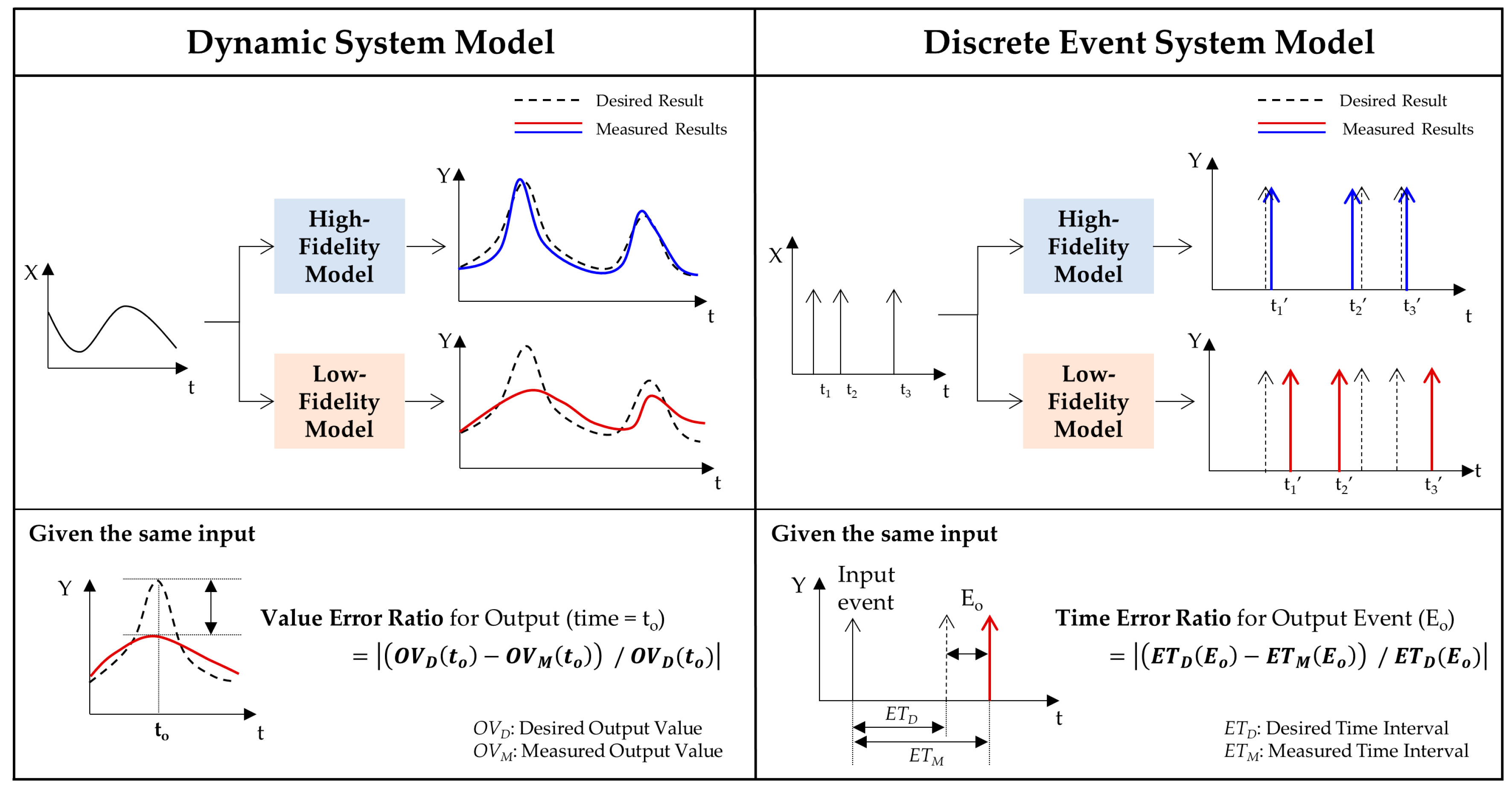
In the simulation world, the level of fidelity is defined as the degree of output similarity between a reference system and a model that abstracts the reference system. Figure 3 illustrates conceptual examples to show the level of fidelity for the target system model: dynamic and discrete event systems. In Figure 3, the desired result is an output of the reference model, which is the reference system itself or the most accurate model compared with the reference system. Fundamentally, outputs of the high-fidelity models (blue lines in Figure 3) are much more similar to the desired outputs compared to those of the low-fidelity models (red lines in the second rows of Figure 3).
To evaluate the fidelity quantitatively, we measure an error between the output of the reference model and that of the target system model, which is classified into two aspects (i.e., time and value). In the dynamic system model, a value error is calculated as the ratio between two output values given the same input. On the other hand, in the discrete event system model, a time error is measured by the difference between time intervals from input to output events given the same input event.
For each aspect, the output error ϵ is defined by the following equation:
In Equation (1), as the root mean square error can be the value error for the dynamic system model or the time error for the discrete event system model. N is the number of samples. For example, N is the number of time samples for the dynamic system model or the number of output events for the discrete event system. The range of is [0, +∞]. If ϵ is close to zero, the outputs of the target model are almost identical with those of the reference model, which means that the target model has a very high fidelity for the samples, N. On the contrary, a large value means that the target model has a low fidelity so that the outputs of the model are distinguished from those of the reference model.
In the DTSS model for the dynamic system, the output values are influenced by the state variables, and the state variables are updated from the state transition function. Therefore, the state transition is closely connected to determining the fidelity of the model. In the DEVS model for the discrete event system, the time of the output is decided in the time advance function. Thus, the time advance function is important in evaluating the fidelity of the model. These functions will be used for developing lower-fidelity models in Section 4.
2.3. Interest Region within a Single Simulation Scenario
A simulation scenario places concepts, attributes, and relations of simulated objects into a dynamic context [29]. The discrete event dynamic system needs a time-based simulation during a specified period suited for satisfactory simulation objectives. The motivated point for multi-fidelity modeling is that the outputs of the low-fidelity model might have little influence on the overall simulation result during a particular simulation period.
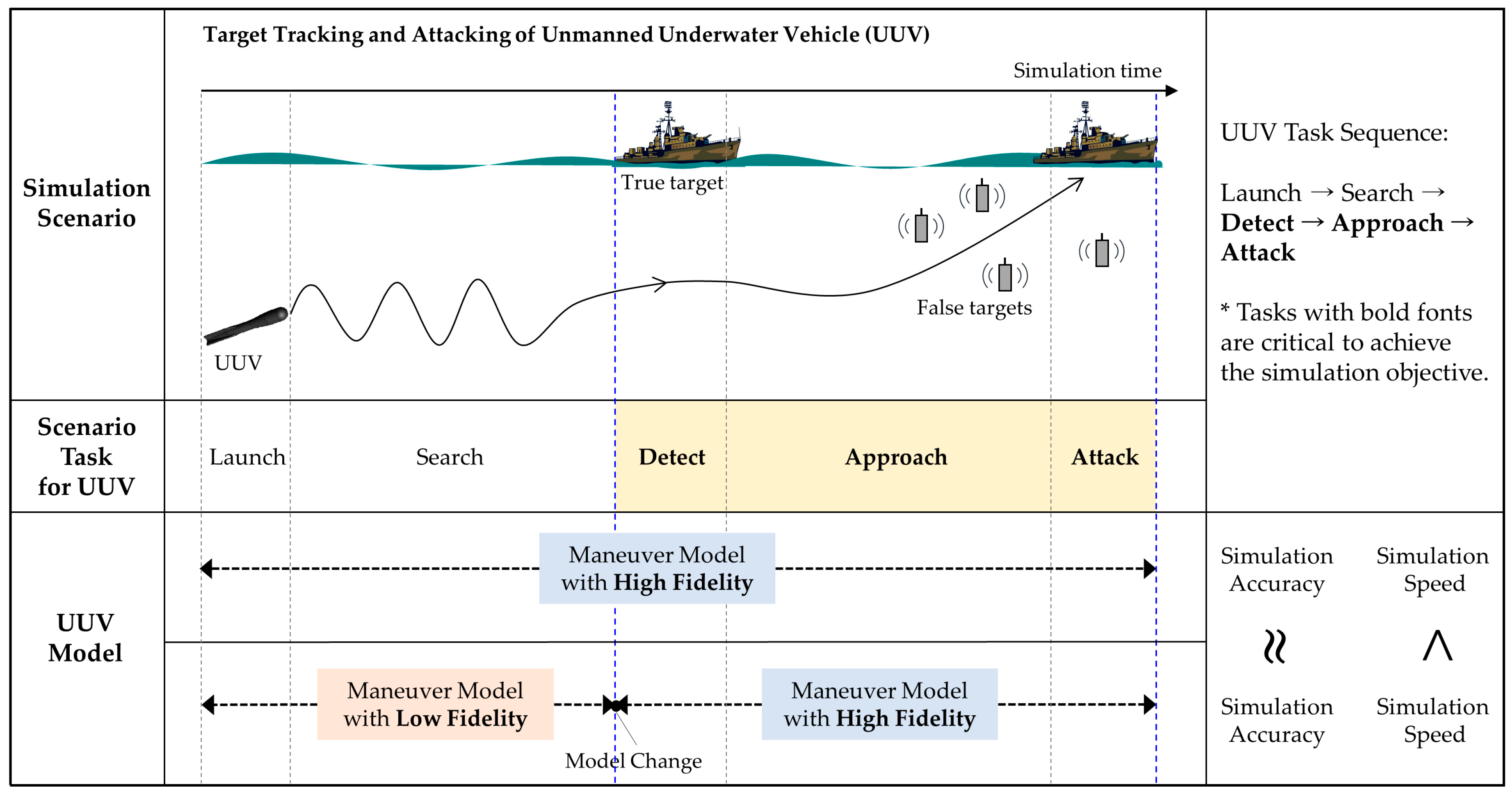
Figure 4 shows an example scenario for tracking and attacking a true target of a UUV. The objective of this simulation is to evaluate a rate of success to attack the target. In this case, the scenario includes a course of action with sequential tasks. First, the UUV is launched and searches for a true target. When the UUV comes closer to a detectable area, it detects the true target. Then, the UUV approaches the true target and attacks it (this scenario will be concretely explained in Section 5). In this scenario, the UUV includes five major tasks: Launch, Search, Detect, Approach, and Attack. Among them, the simulation objective is considered, and the critical tasks are Detect, Approach, and Attack. That is, the low-fidelity outputs of the UUV model in Launch and Search have little effect on the overall simulation accuracy, whereas the outputs in Detect, Approach, and Attack are likely to have a serious impact on the overall accuracy.
This paper proposes an interest region that is a portion of the whole scenario where the model output has a serious effect on the overall simulation analysis. In the example of Figure 4, the interest region is an interval when Detect, Approach, and Attack tasks are conducted. Thus, only the high-fidelity model is employed in this region and lower-fidelity models are used in the remaining parts. The fidelity of the target model is changed based on the interest region during the simulation. With this concept, the simulation result will be very similar to using the high-fidelity model for all intervals; furthermore, simulation speedup will be achieved.
3. Literature Review
Over the last decade, several studies have sought to use multi-fidelity M&S to speed up simulations. The fundamental concept for these studies is multi-fidelity optimization, where lower-fidelity simulations are used to approximate the behavior of the high-fidelity simulation.
For example, Viana et al. [30] used multi-fidelity approximations combined with heuristic methods for the optimal design of aircraft pressure bulkheads. They coupled nonlinear high-fidelity analysis and linear low-fidelity analysis with four methods (i.e., ant colony optimization, genetic algorithm, particle swarm optimization, and life cycle model). Zheng et al. [31] introduced several applications, such as an airfoil wing simulation, car crash simulation, and an artificial neural network, etc., which were achieved with multi-fidelity modeling and an approximation management framework.
Sun et al. [32] proposed a two-stage multi-fidelity procedure for solving crashworthiness design for cellular structures and materials. In the first stage of their proposed work, a correction response surface was constructed based on the ratio between high-fidelity and low-fidelity analyses at a few sample points. In the second stage, low-fidelity analysis is replaced with a radial bias function approximation. Xu et al. [33] presented an ordinal transformation approach to transform the original solution space into a one-dimensional space based on the rankings of solutions using the low-fidelity model. After that, they used an optimal sampling approach to search solutions in the transformed one-dimensional space for optimal solutions using high-fidelity simulations.
One of the common points of the above-mentioned studies is to drive the preliminary design process using low-fidelity models as surrogates for expensive high-fidelity simulations. Then, high-fidelity models are employed in the final design stages to refine the design. In this case, the multi-fidelity technique is to utilize initial design points determined from a low-fidelity simulation to correct the simulation at other design points. This means that the fidelity did not change dynamically during the same simulation scenario. In addition, because these studies have focused on application-based approaches to resolve practical issues, there has been no formal representation of the multi-fidelity model and no model reusability of existing simulation models.
Williams and Alleyne [34] presented a modeling framework for dynamically changing the fidelity of component models throughout a single scenario–the approach most similar to our own. For a dynamic change of fidelity, they proposed the following design concepts: (1) a supervisor filter to analyze and determine which inputs trigger a switch to low- and high-fidelity models and (2) a dwell time that provides a buffer during fidelity switching. The proposed framework was demonstrated for a finite-volume model of a vapor compression system where the model fidelity is based on the number of volumes used for the evaporator. Although the authors regarded dynamic changes of the fidelity, this study also suffers from an insufficient representation of behaviors of the event-based system. For example, the authors did not consider internal discrete events of the model but focused on exogenous signals; thus, the modeling form used in Williams and Alleyne’s study also makes it difficult to directly apply it to the discrete event dynamic system.
In common with most M&S methods, multi-fidelity M&S inevitably involves behavioral errors of the developed models due to their approximations. Cassettari et al. [35] classified them into two types. The first error is directly connected to the translation of the real system into a simulation model; the second one is related to the transformation of the simulation models. In multi-fidelity M&S, the high-fidelity model facilitates reducing the first error, whereas the lower-fidelity models make the second error in place of enhancing simulation speedup. To minimize the second error, in this paper, we only use lower-fidelity models for the marginal parts of a single scenario. As we explained in the introduction, the single simulation scenario does not need to be simulated with high-fidelity models. For example, if a simulation analysis for one-day traffic is carried out, it is highly effective to focus on analyzing traffic during rush hour. Therefore, the high-fidelity models are primarily used for important regions of the scenario, whereas the lower-fidelity models are used for marginal parts. With this concept, this paper proposes a general framework for multi-fidelity modeling for enhancing simulation speed while minimizing accuracy loss and maximizing model reusability. We will show these points with empirical simulation results in Section 5.
4. Proposed Framework
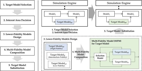
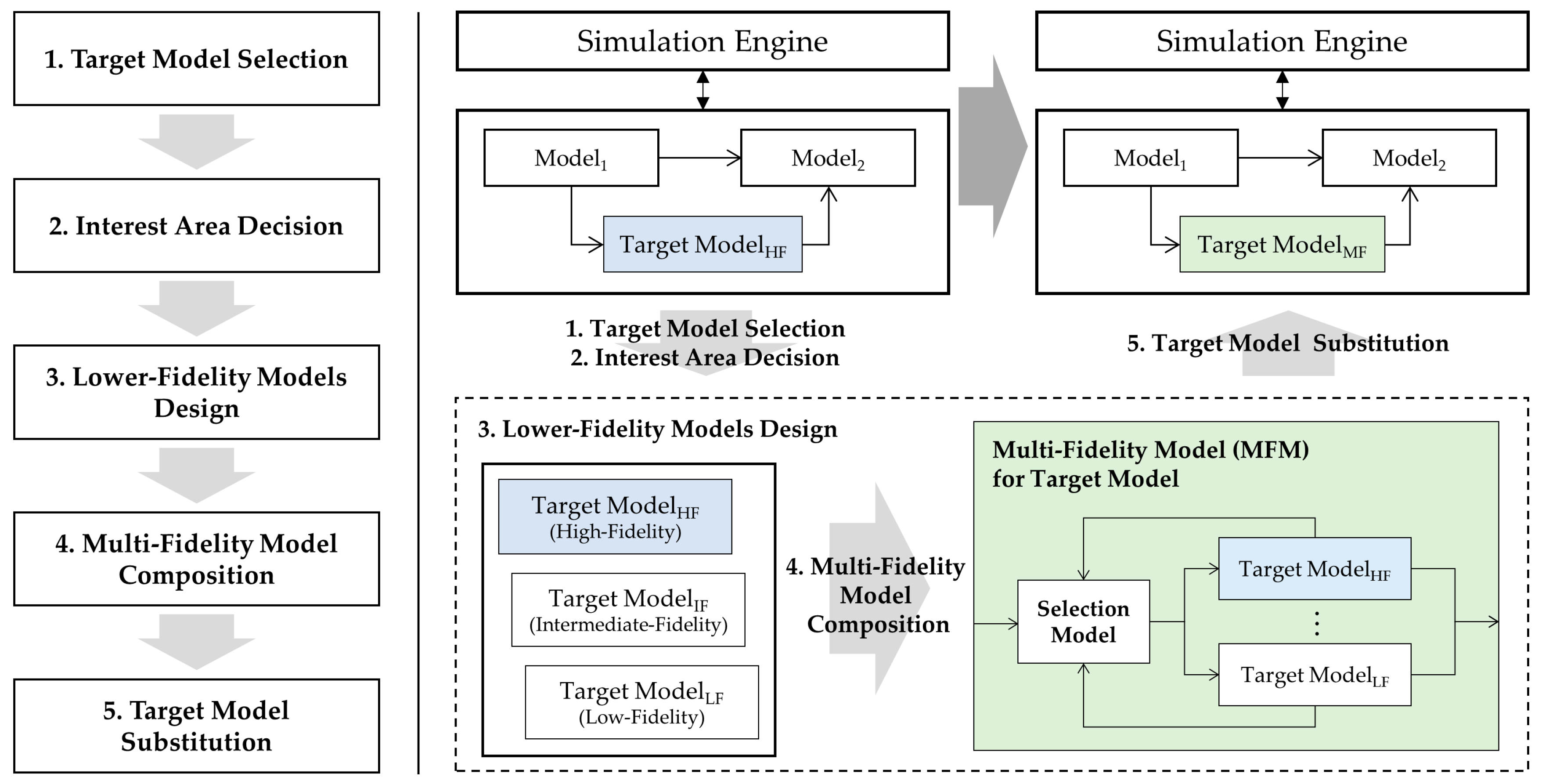
This section proposes the overall procedure for the multi-fidelity modeling framework. As depicted in the left diagram of Figure 5, the framework consists of the following five steps: (1) target model selection, (2) interest region definition, (3) lower-fidelity model design, (4) multi-fidelity model composition, and (5) selected target model substitution. In this framework, we assume that the target model already has a high fidelity (Target ModelHF in Figure 5 are relevant here). Based on the high-fidelity model, lower-fidelity models for the target model (e.g., Target ModelIF and Target ModelLF) are additionally developed for simulations in non-interest regions. A multi-fidelity model (e.g., Target ModelMF) contains a selection model to choose a proper model from among the models with variable fidelities. With regard to a systemic aspect, the input and output variables of the existing target model are equal to those of the multi-fidelity model that is substituted for the model (see Target ModelHF and Target ModelMF in Figure 5). This guarantees the reuse of other existing models and the simulation engine minimizing modifications.
In the following subsections, we will explain the steps in detail and describe the evaluation index for simulation speedup.
4.1. Target Model Selection and Interest Region Definition
The first step of the proposed framework is to choose a target sub-model from the entire simulation model. The selected model should satisfy the following two prerequisites: (1) it is modeled by the DTSS or DEVS formalism and (2) it fundamentally has high fidelity with computational complexity and is executed frequently during the simulation.
Next, we define an interest region of the target model. As we explained in Section 2.3, the interest region is a part of the whole simulation scenario where the model output has a serious effect on the overall simulation analysis. The definition of the interest region simplifies how the framework achieves multi-fidelity modeling: the high-fidelity model is exclusively simulated within the interest region of the whole scenario. If the overall scenario is designated as a large interest region, the high-fidelity model is fully simulated without using lower-fidelity models, which means that changes of the model’s fidelity do not occur within the scenario.
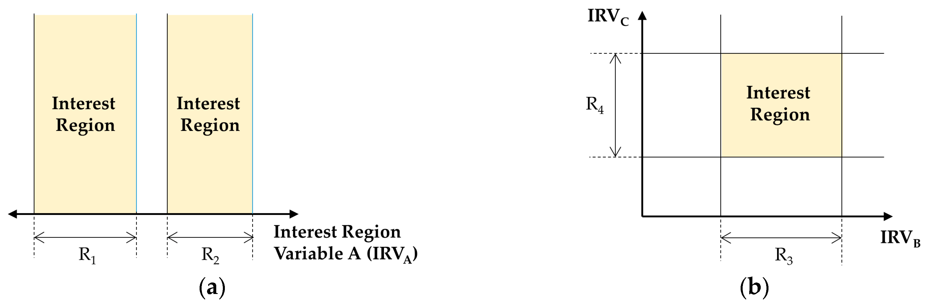
Figure 6 shows two examples for setting up the interest region. Because our target system is a discrete event dynamic system, which is represented with either the DEVS or DTSS model, the simulation is a process of updating input, state, and output variables as time progresses. In this context, the interest region is an acceptable range of the input and state variables of the target model. Figure 6a shows that two regions are set up with two ranges (i.e., R1 and R2) for one interest region variable (IRVA); Figure 6b represents just one region to intersect two ranges for two variables (i.e., R3 for IRVB and R4 for IRVC).
4.2. Lower-Fidelity Model Design
The third step is to develop lower-fidelity models for the selected target model. We will explain this step by distinguishing between dynamic and discrete event system models.
4.2.1. Lower-Fidelity Models Design for the Dynamic System
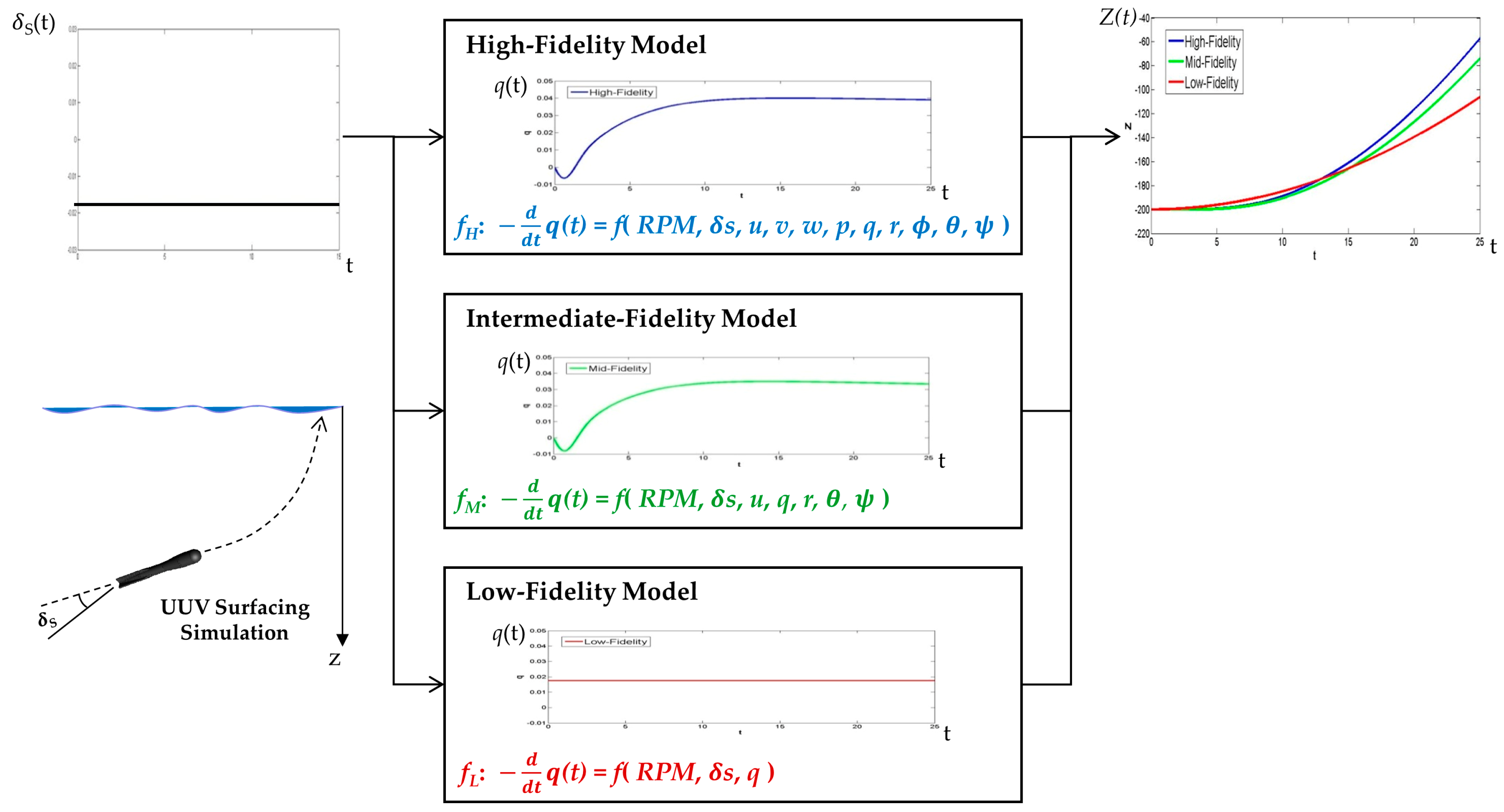
As mentioned in Section 2, the fidelity of the DTSS model is determined by the state transition function. Therefore, lower-fidelity models are designed to simplify this function of the current target model that already has a high fidelity. For simplification of the function, this paper suggests two methods: elimination and projection. The elimination method deletes the terms that have little effect on the accuracy of output in the state transition function and the projection method fixes the values of variables in the state transition function.
Figure 7 shows an example of lower-fidelity model design for a UUV surfacing simulation. The target model is the maneuver model for UUV motion in six degrees of freedom. We assume that the input of the UUV maneuver model is an elevator S(t), the output is a depth Z(t), and one of the state variables is a pitch q(t). The state transition function of the model is a differential equation, which consists of many terms. Further explanations for the maneuver equation are found in [36]. Depending on the level of eliminating terms, an intermediate-fidelity model and a low-fidelity model can be developed by using the elimination method, which is used to derive fM and fL from fH and fM, respectively. The more terms that are eliminated, the more the accuracy of the state and out variables decreases.
Table 1 shows empirical results regarding the simulation execution time and simulation accuracy for the above example. We first measured the elapsed time for a single simulation. The simulation of the high-fidelity model took about twice as much execution time as the low-fidelity model. For example, if the number of iterations of this simulation is more than 500,000, the high-fidelity model’s simulation takes twenty-three more days than that of the low-fidelity model. We next calculated ϵ derived from Equation (1). In this experiment, the desired result is obtained from the high-fidelity model (this means that the reference model is the high-fidelity model fH). For simulation accuracy, the high-fidelity and the intermediate-fidelity models had similar ϵ values; however, the low-fidelity model had an value with a significant difference.
4.2.2. Lower-Fidelity Models Design for the Discrete Event System
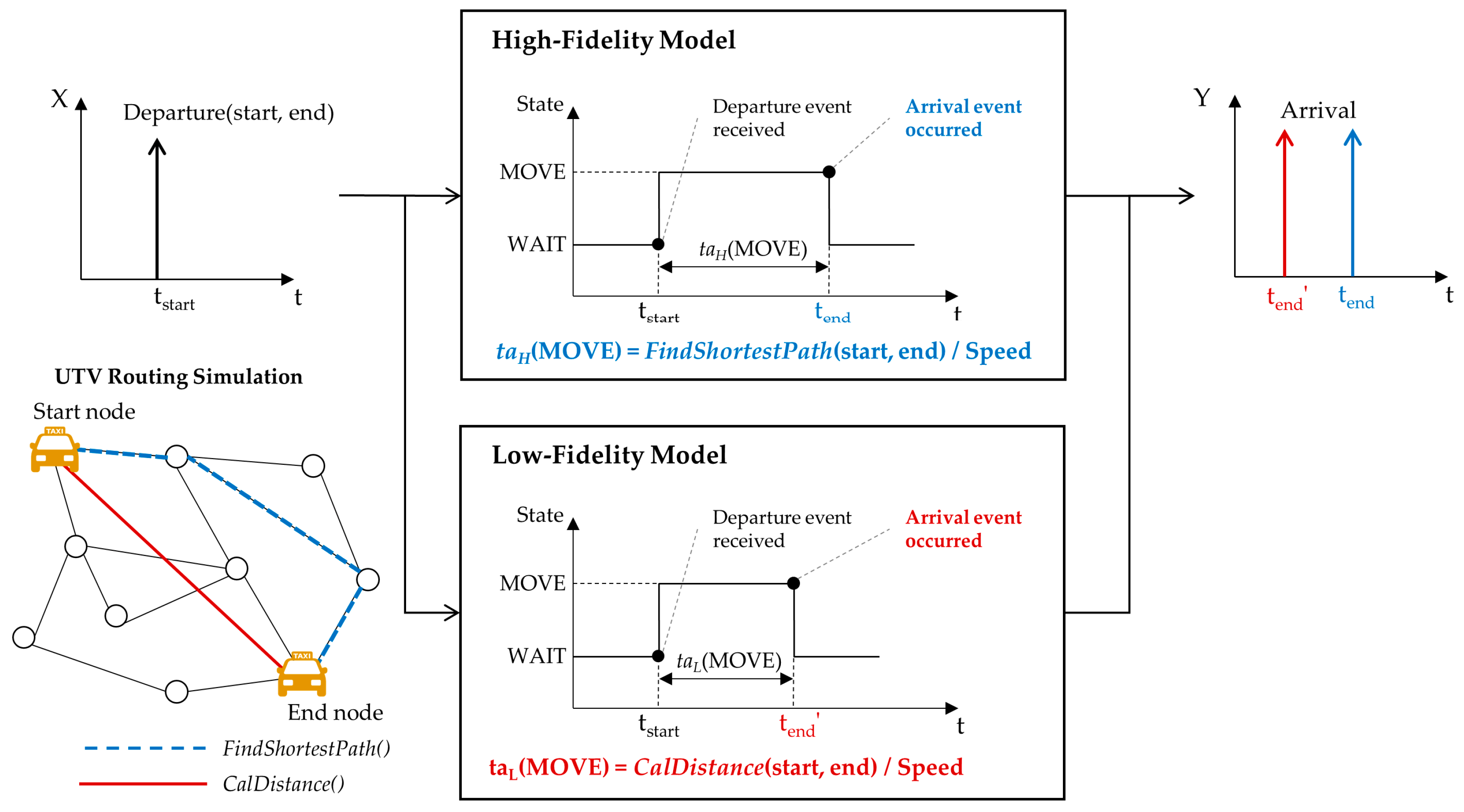
In the discrete event system, lower-fidelity models are designed to simplify the time advance function of the DEVS model. We explained high- and low-fidelity models for the UTV, which is shown in Figure 8. The UTV brings passengers to their destinations via the fastest route; thus, its DEVS model computes the duration time from pickup to drop-off, which is carried out by the time advance function. In Figure 8, when the UTV model receives an input event, Departure, the model changes the state to MOVE from WAIT. Then, the model computes the time of the state, MOVE, to generate the output event. The high-fidelity model calculates it by using the Dijkstra algorithm [37], which finds the shortest path from a start node to an end node in a map with several nodes and their connections. However, the Dijkstra algorithm has computational complexity and the increase in computational cost is exponentially related to the number of nodes. The low-fidelity model uses a simple algorithm that just calculates the travel time of the straight-line distance between the start and end nodes. The accuracy of this simple algorithm is lower than that of the Dijkstra algorithm, though its calculation speed is much faster than that of the Dijkstra algorith.
We measured the execution time and for 2000 input events, as shown in Table 2. The simulation of the low-fidelity model was approximately seven times faster than the case of the high-fidelity model; however, for the low-fidelity model was 0.21 higher than that of the high-fidelity model. , which was measured in these two simple examples, is a theoretical measurement focusing on the target model itself, not the overall simulation model. Because the target model is a sub-model of the whole model, we will evaluate the simulation accuracy from the view of the overall simulation objective in Section 5.
4.3. Multi-Fidelity Model Composition and Target Model Substitution
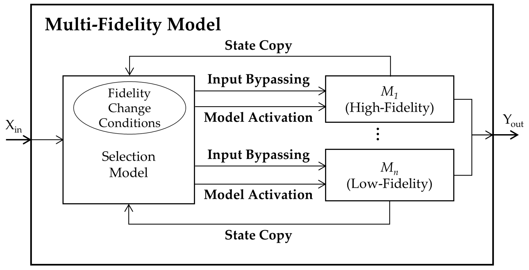
After the development of lower-fidelity models for the target model, we needed to composite a multi-fidelity model (MFM). For composition, the formal structure of the MFM is illustrated in Figure 9. The MFM consists of two types of models: internal target models and a selection model. The original target model and its derived models with lower-fidelity correspond to the internal target models. A selection model determines an appropriate internal model for each predefined region, which implies that, among the several internal models, only one model is activated for each simulation time.
To be specific, the selection model has two important roles. When the selection model receives an input (Xin in Figure 9) from outside of the MFM, it decides whether the current internal model needs to be changed based on the FCC. First, if the model requires no change, the selection model sends the input to the model. The internal model carries out its own actions and generates two outputs: an actual model result for the input (Yout) and its current state. The current state is transferred to the selection model. These are the cases of the input bypassing and the state copy, as shown in Figure 9. Otherwise, if a model change is required, the selection model activates the other model by sending the input Xin with the copied state for continued simulation. This is relevant to the model activation in Figure 9. In this way, the selection model will manage the trade-off between the computational resources and the accuracy of the simulation results. Specifically, it will decrease the computational burden in noncritical regions while increasing the simulation accuracy in critical regions. The specification for the MFM is described as follows.
- is the set of inputs;
- is the set of outputs;
- is the set of models with variable fidelities;
- is the selection model;
- is the model coupling scheme;
- is the external input coupling;
- is the external output coupling;
- is the internal coupling.
4.3.1. Multi-Fidelity Model Composition for Dynamic System
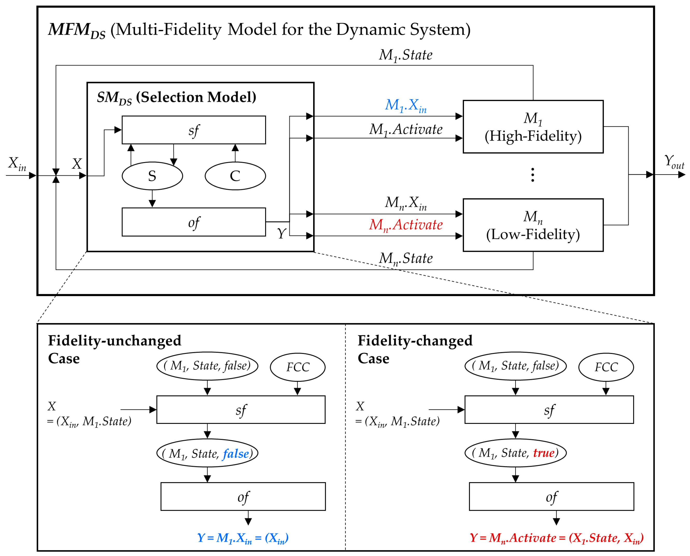
Figure 10 shows the structure of the multi-fidelity model of the dynamic system. The internal models (i.e., M1 to Mn) are expressed with the DTSS formalism mentioned in Section 2; the SMDS has a similar form to the DTSS so that overall models can be simulated with the existing simulation engine.
- is the set of inputs;
- is the current state input of internal model ;
- is the set of outputs;
- is the set of bypassing outputs to ;
- is the set of activating outputs to ;
- is the set of internal model states;
- is the set of fidelity change conditions;
- is the selection function;
- is the output function.
The specification of the SMDS is given after Figure 10. The SMDS has two types of input sets: an external input set from outside of the MFMDS and a state input set. The two types of output sets for input bypassing and model activation are allowed by the SMDS. Fundamentally, the SMDS receives the external input Xin, and sends it to a current internal model Mi in the form of the output Mi.Xin. The SMDS receives the state input Xi.State from the Mi and checks whether a model change is needed. If a change is required, the SMDS sends the output for model activation Mj.Activate to the altered model Mj. The SMDS has two sets of states: (1) a set of internal model states including the current internal model, the state variable of the model, and the Boolean variable to check whether there has been a model change; and (2) a set of fidelity change conditions. Finally, the SMDS employs two functions: a selection function sf and an output function of. The sf, which is mapped to the state transition function of the DTSS model, decides whether the current internal model is changed with the FCC when the SMDS receives an external input. If the current internal model does not need to be changed, the of sends the external input to the model. Otherwise, the of sends the state of the current internal model and the external input to the altered internal model (blue fonts are relevant to the fidelity-unchanged case and red ones correspond to the fidelity-changed case in Figure 10).
4.3.2. Multi-Fidelity Model Composition for Discrete Event System
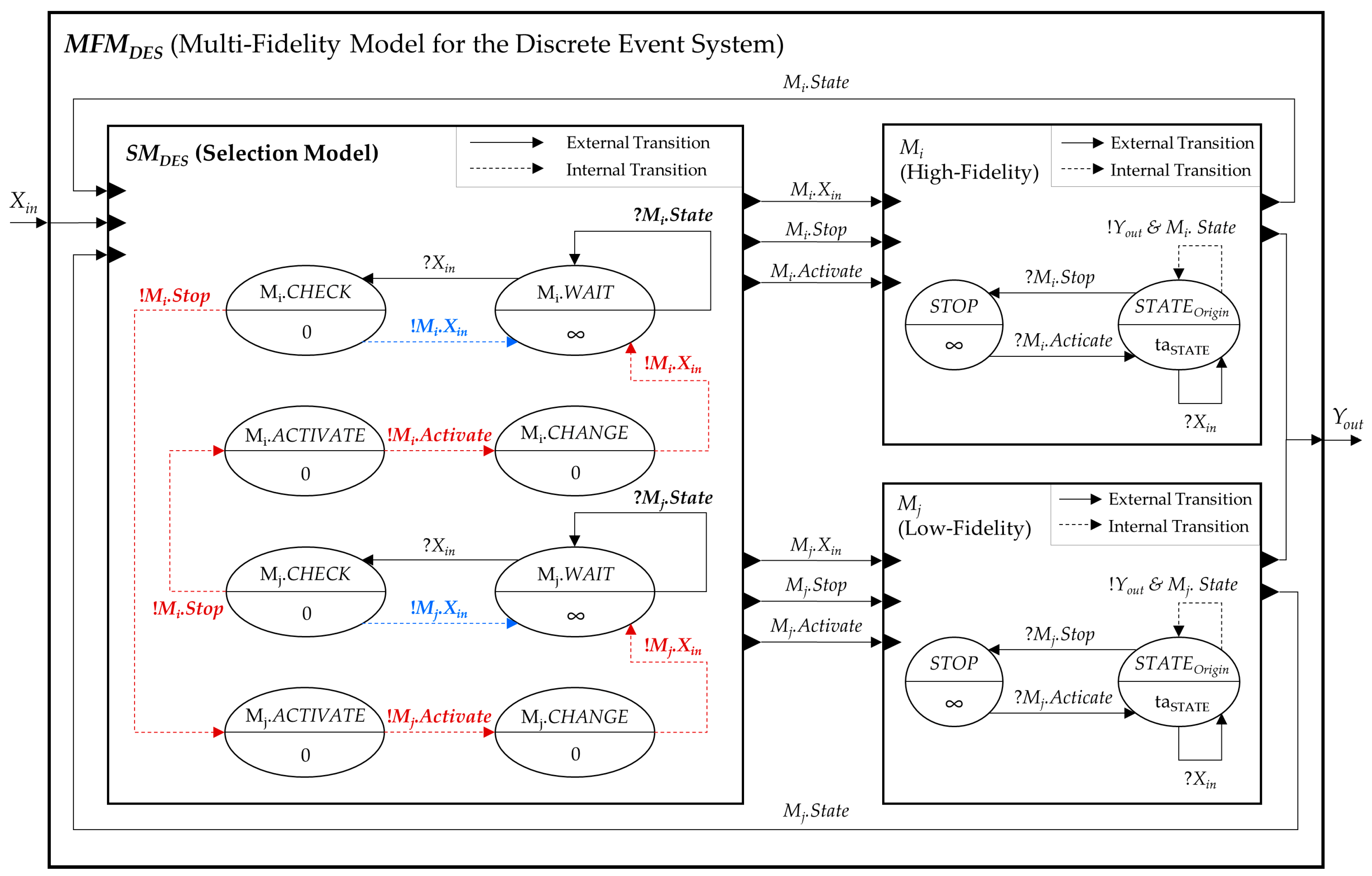
The structure of the multi-fidelity model of the discrete event system is shown in Figure 11. All the models in the MFMDES are designed with the DEVS formalism [18]. Unlike the DTSS model, the DEVS model can be executed regardless of whether it receives an input event or not. Thus, the MFMDES has an additional output event Mi.Stop to stop the execution of the current internal model Mi when another internal model needs to be activated. If the current model receives the input event Mi.Stop, it enters the STOP state, which is an additional state in which the state time is infinite, and waits for the next activation. When the Mi receives the activate event afterward Mi.Activate, the Mi returns to the previous state before it is deactivated StateOrigin. The specification is a formal representation of the selection model SMDES.
- is the set of inputs;
- is the current state input of internal model ;
- is the set of outputs;
- is the bypassing output of ;
- is the activate output of ;
- is the stop output of .
- is the set of fidelity change conditions.
- ;
- ;
- ;
- ;
- ;
- ;
- ;
- ;
- ;
- ;
- ;
Except for the stop event, the input and output sets of the SMDES are identical to those of the SMDS. The SMDES has two sets of states (i.e., FCC and S). The FCC is the same as that of SMDS, whereas the S is slightly different. In the SMDES, the S is mapped to four phase sets—Mi.WAIT, Mi.CHECK, Mi.ACTIVE, and Mi.CHANGE. Unlike the SMDS, two important roles of SMDES are conducted by a series of phase transitions. The basic phase is Mi.WAIT, assuming that the current internal model is Mi. When the SMDES receives the input event Xin from the Mi, it moves the phase into Mi.CHECK and checks whether the activated model is changed to the Mj based on the sf and the FCC. As in the first case, if the current internal model Mi needs to remain active, the SMDES changes its phase to Mi.WAIT and forwards the received input Xin to the Mi. In another case, if the Mi needs to be changed, the SMDES moves the phase to Mj.ACTIVE—according to the next activation model, Mj—and sends the stop event Mi.Stop to the Mi. Then, the SMDES moves the phase to Mj.CHANGE to send the activation event Mj.Activate to the Mj. Finally, the phase of the SMDES changes to Mj.WAIT, and SMDES sends the Xin to the current internal model Mj. In either case, the SMDES receives the state information from the current activated model and waits until another input Xin arrives. A sequence of transitions of the phase, the input, and the output for input bypassing is as follows (parentheses contain the output message, ⟹ means the external transition, and ⟶ means the internal transition):
Additionally, a series of phase transitions for the model change is as follows (inputs and outputs in red fonts in Figure 11 are relevant to this sequence):
Finally, the MFM substitutes the target model with minimal modifications of the other models. Small modifications used to add more messages—and the STOP state, in the case of the DEVS model—are unrelated to model logic, as they are just subsidiary functions.
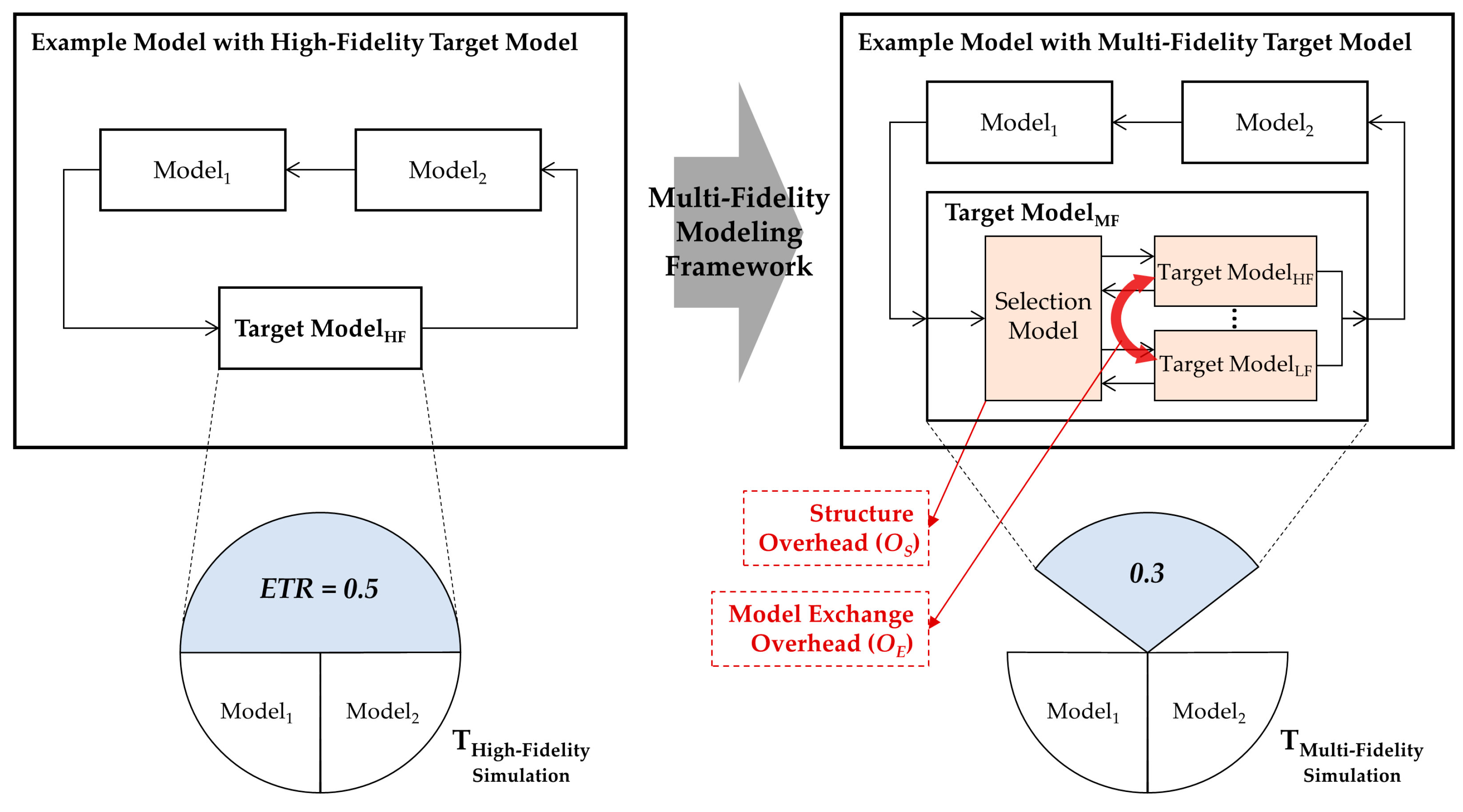
4.4. Evaluation Index for Simulation Speedup
The simulation speed improvement obtained by applying the proposed multi-fidelity framework is defined as follows:
ETR is the percentage of execution time of the target model in the overall simulation execution time. and are the coefficients for the structure overhead and model exchange overhead in the selection model, respectively. The value of is greater than 1, and has a value between 0 and 1. For each model in the multi-fidelity model, is the ratio of execution time of to the execution time of the target model, and is the percentage at which is simulated in the entire simulation scenario (). That is, implies the actual ratio of execution time of in the multi-fidelity model. When is the same as the target model, the value of is 1, and is the percentage of the interest region in the scenario. Figure 12 illustrates the speedup of the proposed framework and the notations in (2). In order to apply the proposed framework more effectively based on (2) (i.e., to maximize the speedup), we first have to select a model with a large ETR as a target model. This corresponds to the second of the two prerequisites in the first step of the target model selection in our framework. Using a variety of fidelity models through appropriate scenario partitioning can minimize , but can lead to increasing the structure overhead ; thus, we have to reduce the overhead by simplifying the selection function sf. In addition, minimizing the frequency of model exchange can increase the speedup by reducing the overhead .
5. Applications
In this section, we discuss two case studies that were applied to the proposed modeling framework: (1) UUV simulation for the dynamic system and (2) UTV simulation for the discrete event system.
5.1. UUV Simulation
The objective of the UUV simulation is to evaluate the success rate for tracking and attacking a real target [38,39]. Because this evaluation is done through a what-if analysis of various situations, including UUV specifications and tactics for tracking and attacking, a large number of repeating simulations are necessary; thus, for a more efficient analysis based on the simulation, we applied the proposed modeling framework to improve simulation speed.
5.1.1. Target Tracking Scenario for UUV
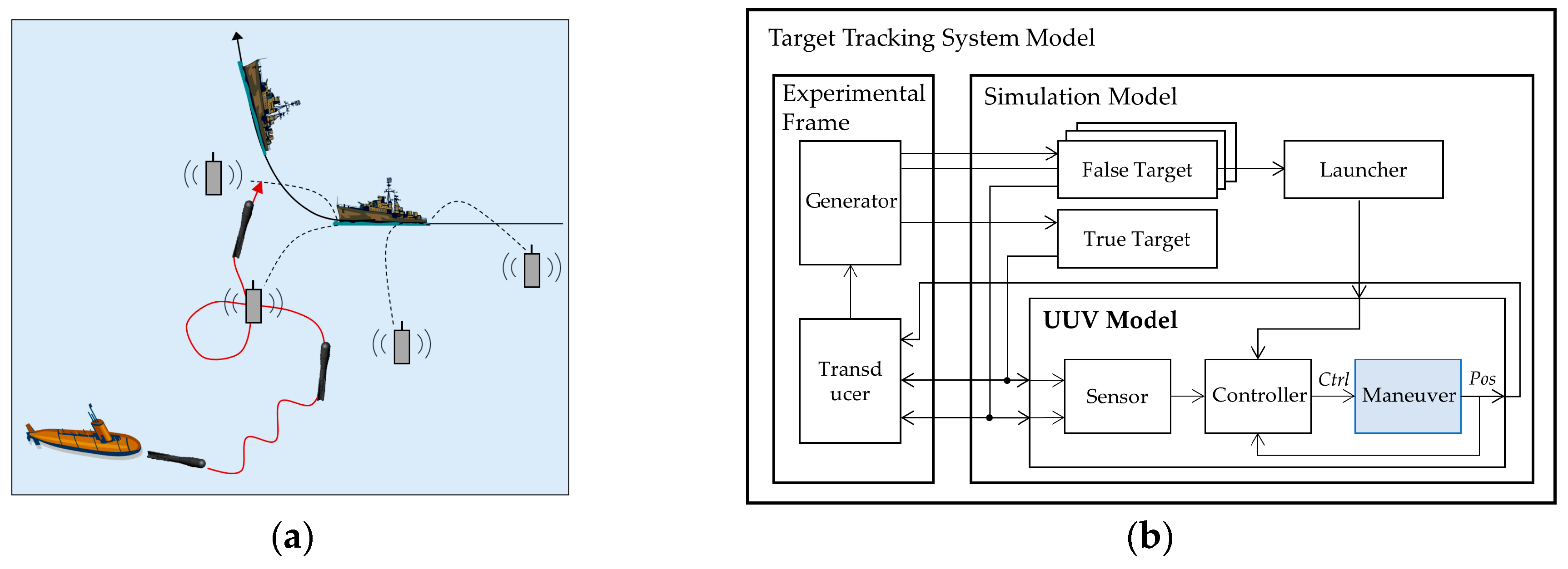
Figure 13a represents a scenario of evaluating the success rate of UUV. A UUV, launched by one vessel toward a warship (i.e., the true target), finds the warship based on its own search tactics. When the UUV finds the warship, it chases the warship with the purpose of attacking it. On the other hand, when the warship detects the approaching UUV, it drops several decoys (i.e., false targets) and runs away. Depending on the specifications of UUV and the attacking tactics, the UUV will either hit the warship by overcoming the disturbance caused by decoys, or fail to hit it and eventually explode. The simulation model structure for this scenario is shown in Figure 13b. All models were based on DTSS and implemented with C++ language.
5.1.2. Multi-Fidelity Modeling Process
As mentioned previously, the first step of our framework is selecting a target model for multi-fidelity modeling. Depending on the two prerequisites for the selection, we chose the maneuver sub-model of the UUV model as the target model, because it is modeled by the DTSS and has the highest ETR: 0.51 (i.e., it requires high computational complexity to solve the six degrees of freedom movement differential equation, and it is executed continuously over the entire simulation time). As a second step of deciding the interest region, we used the state variable of “bDetect” in the UUV model as the IRV. It is a Boolean variable that represents whether the UUV detects the target. After its value has changed to true, the UUV traces the target to attack, and the movement of the UUV (the output of the maneuver model) at this time greatly affects the success rate, the simulation result; thus, the interest region of the maneuver model was defined when “bDetect” was true (see Figure 4 in detail).
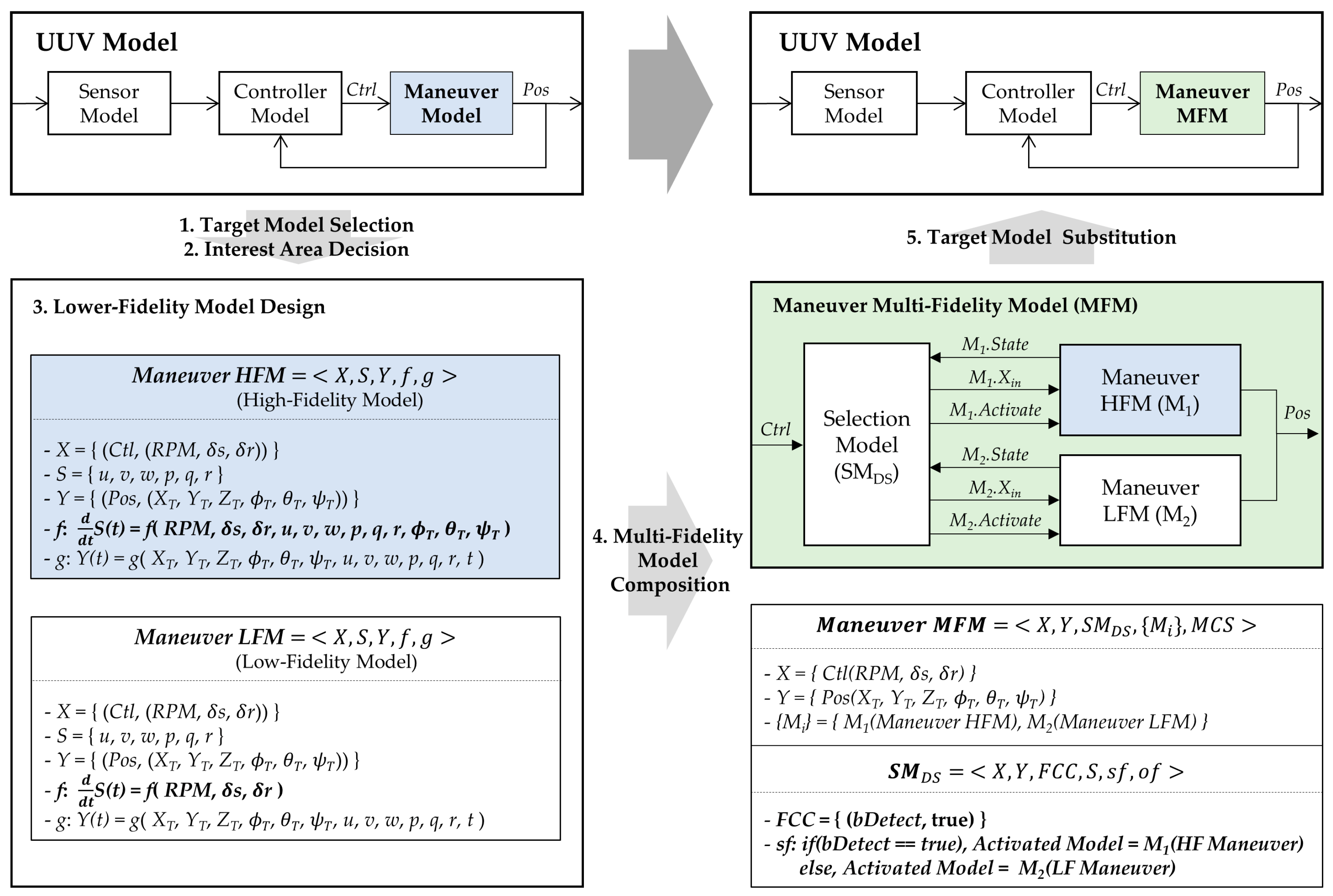
The third step is to develop a lower-fidelity model of the target model. The state transition function of the target model uses differential equations to calculate the change amount of the state variables while considering various physical effects: e.g., thrust force, gravity force, and drag force, etc. [16]. We developed the low-fidelity maneuver model by simplifying this transition function with the elimination and projection methods, as shown in Figure 14. Concretely, we eliminated several terms related to , , and that have little effect on the accuracy of the output of the function, and projected , , and to proportional values of , , and .
The fourth step is to composite a multi-fidelity model based on the specifications in Section 4.3.1, as shown in Figure 14. The high-fidelity model is the existing maneuver model, and the low-fidelity model is the developed lower-fidelity model in the previous step. According to the interest region of the target model defined in the second step, FCC is composed with “bDetect” and its value: true. The last step is to substitute the target model with the composed multi-fidelity model without any modifications of the other models in the UUV simulation model.
5.1.3. Simulation Results
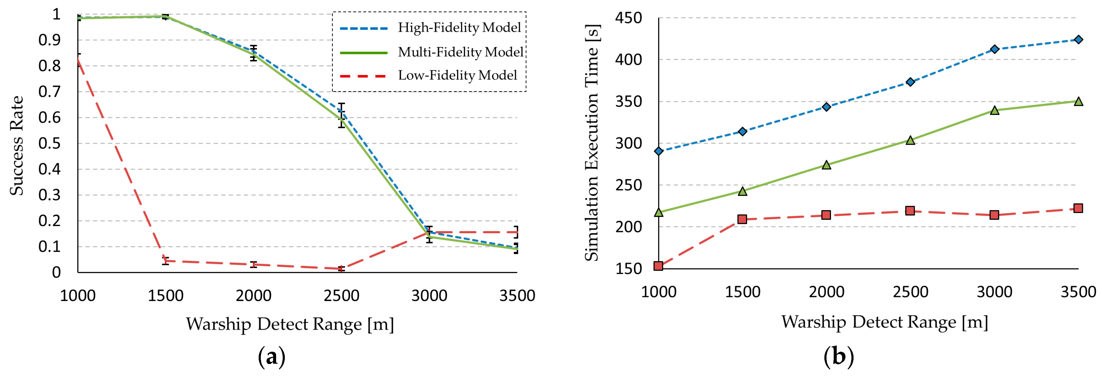
The success rate of UUV can be evaluated in various situations; however, in this case study, we evaluated this rate according to the various detection ranges of the warship. To demonstrate the effectiveness of the proposed multi-fidelity framework, we compared the developed multi-fidelity model with the existing UUV simulation model (i.e., the high-fidelity model) and the low-fidelity model. The low-fidelity model is a simulation model in which the maneuver model is replaced with the low-fidelity maneuver model. Figure 15 represents the success rate and execution time of the UUV simulation models with different fidelities. To achieve a standard error within 0.031 and a confidence level of 95%, the UUV success rate and the execution time were evaluated using 1,000 time-independent repeating simulations. As shown in Figure 15, the execution time of the multi-fidelity model is lower than that of the high-fidelity model while the success rate of the multi-fidelity model is almost the same as that of the high-fidelity model. On the other hand, the execution time of the low-fidelity model is much lower than that of the high-fidelity model and multi-fidelity model while its success rate is very different from the others. Based on the simulation speedup defined in Section 4.4, applying the proposed framework increases the speed about 1.25 times without a significant loss in the accuracy of the success rate and without modifying the simulation engine and the other existing models.
5.2. UTV Simulation
The objective of the UTV simulation is to evaluate the average waiting time of passengers and the average utilization rate of vehicles. To decide the optimal number of vehicles based on the UTV simulation, we need to evaluate the waiting time and utilization rate through many iterative simulations for various parameters, such as the organization of roads, the distribution of passengers, the speed of vehicles, etc.; thus, we applied the proposed multi-fidelity modeling framework to improve the UTV simulation speed.
5.2.1. UTV Simulation Model
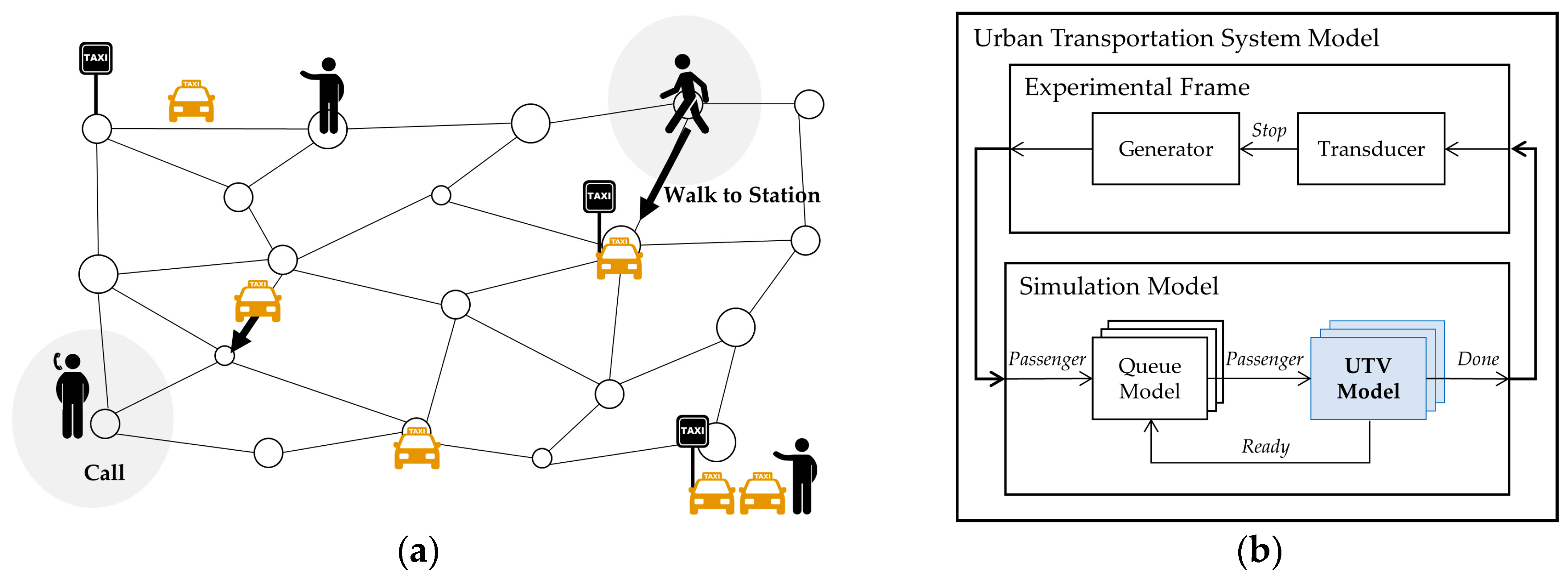
Figure 16a represents a UTV simulation scenario. Roads and intersections are represented by edges and vertices of the graph. Some vertices have vehicle stations. Passengers are randomly generated at each vertex. If a station is near the vertex where a passenger is generated, the passenger goes to the station and takes a vehicle in the station. Otherwise, the passenger calls a vehicle, and the closest vehicle is allocated to the passenger. If no vehicles are in the station, the passenger waits for a vehicle or calls a vehicle. When a vehicle picks up a passenger, the vehicle goes to the passenger’s destination vertex. After dropping the passenger at the destination, the vehicle goes to the nearest station and waits for passengers. The simulation model structure for this UTV scenario is shown in Figure 16b. Each queue model and UTV model represents the station and the vehicle. The UTV model is an agent model that decides and acts according to the several rules described in the scenario. All models were based on DEVS and implemented with DEVSim++ [40].
5.2.2. Multi-Fidelity Modeling Process
The first step is selecting a target model for multi-fidelity modeling. Based on the two prerequisites for the selection, we chose the UTV model as the target model, because it is modeled by the DEVS and has the highest ETR: 0.98 (i.e., it requires high computational complexity to find the shortest path using the Dijkstra algorithm, and it is executed continuously over the entire simulation time). To choose the interest region of the UTV model, we used the state variable of “Distance” as the IRV. It is a positive number that represents the expected distance between a passenger’s departure vertex and arrival vertex. In the UTV simulation, the shortest path of a vehicle has a great effect on the accuracy of the simulation results. As the expected distance increases, the shortest path found by the Dijkstra algorithm becomes more complex; thus, the interest region of the UTV model was defined when “Distance” had a high value. However, the exact criteria for this high value can vary depending on the low-fidelity model. In this case study, we decided this value experimentally with a consideration of the trade-off relation between the execution time of the UTV simulation and the accuracy of the simulation results (see the fourth step of the applied framework).
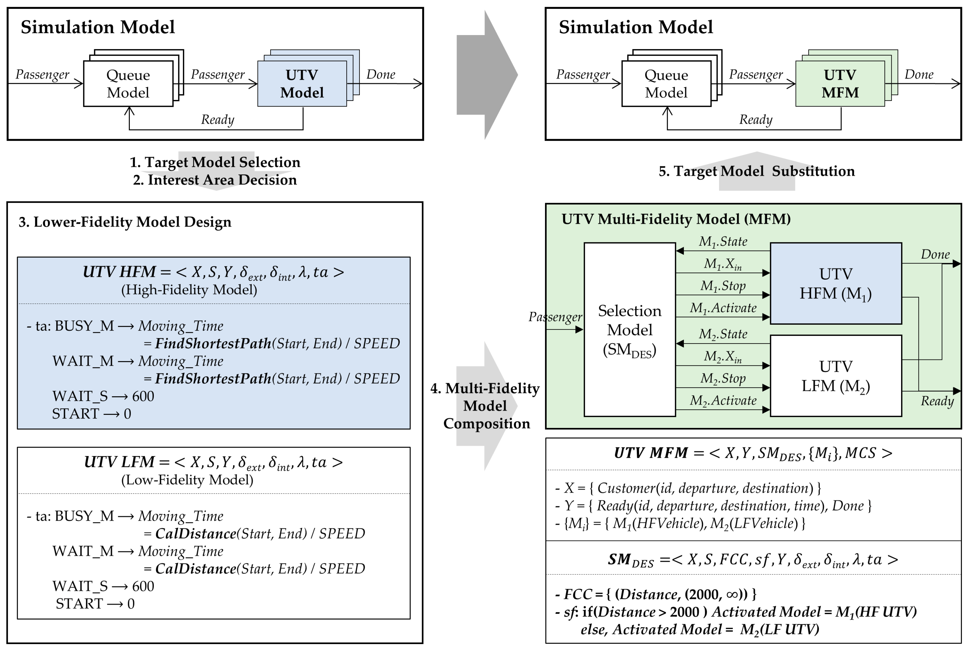
The third step is to develop a lower-fidelity model of the target model. We developed the low-fidelity UTV model by simplifying the time advance function, as shown in Figure 8. The existing UTV model (i.e., the high-fidelity model) calculates the state time of “BUSY_M” and “WAIT_M” using the shortest path found by the Dijkstra algorithm, whereas the low-fidelity model simply uses the Euclidean distance between the starting and ending vertex. The fourth step is to composite a multi-fidelity model based on the specification in Section 4.3.2, as shown in Figure 17. The high-fidelity model is the existing UTV model, and the low-fidelity model is the developed lower-fidelity model in the third step. As mentioned previously, we have to decide the exact value that separates the interest region to determine the FCC.
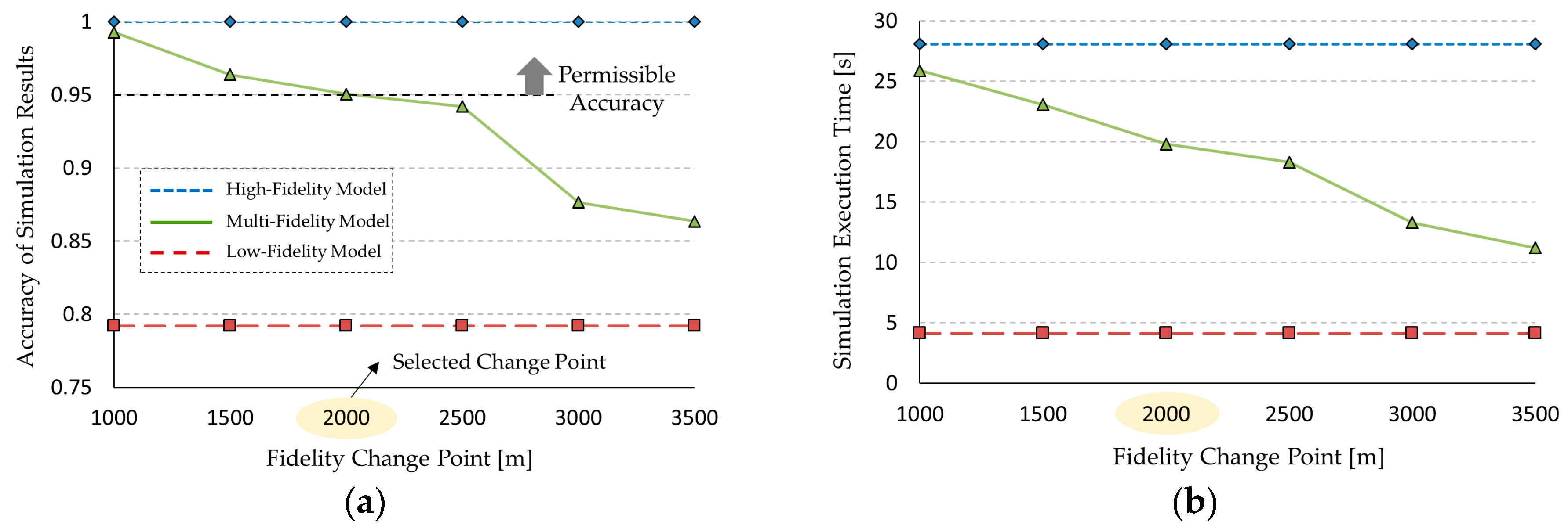
To this end, for the composited multi-fidelity model, we measured the simulation execution time and the accuracy of the simulation results according to the various fidelity change values of “Distance”, as shown in Figure 18. The accuracy here is the relative accuracy to the existing UTV simulation model (i.e., the high-fidelity model). As the change value increases, the number of executions of the low-fidelity model increases in the multi-fidelity UTV model; thus, the execution time decreases, but the accuracy is also lowered. Assuming that the permissible accuracy loss is under 0.05, the possible candidates for the change value are 1000, 1500, and 2000. To maximize the speedup of the multi-fidelity model, the change value was decided as 2000 with the minimum execution time. As a result, the FCC was composed with “Distance” and its value: 2000. The last step is to substitute the existing UTV model with the composed multi-fidelity model without any modifications to the other models in the UTV simulation model.
5.2.3. Simulation Results
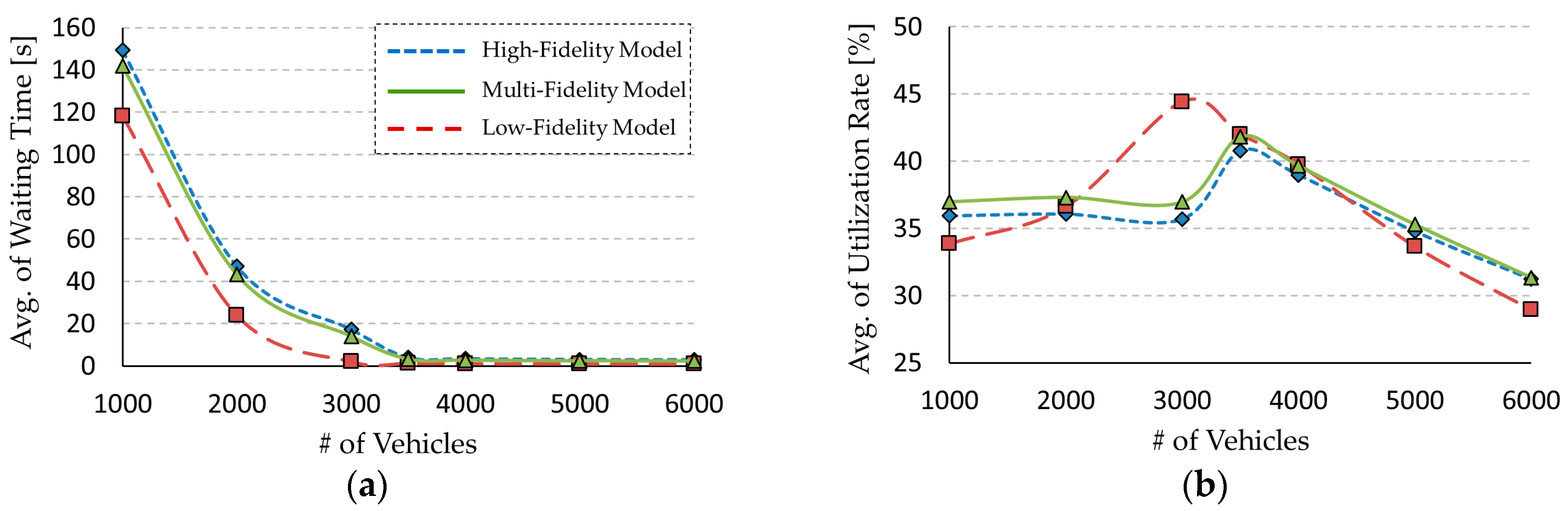
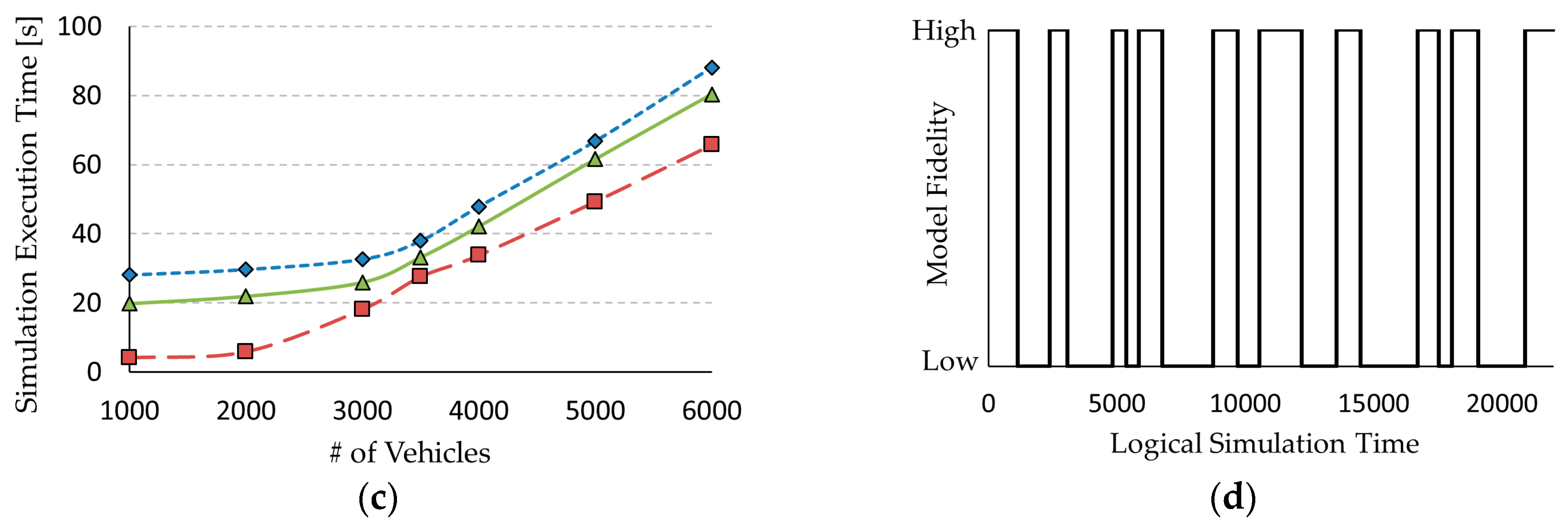
In this case study, the parameters of the UTV simulation model were set based on real map data and a domestic report to increase the reliability of the simulation results. According to the various number of vehicles, Figure 19 represents the average waiting time of passengers, the average utilization rate of vehicles, and the execution time of the UTV simulation models with different fidelities. The meanings of the high-, low-, and multi-fidelity models are the same as those in the previous case study. The results in Figure 19 demonstrate the effectiveness of the proposed multi-fidelity framework. The execution time of the multi-fidelity model is lower than that of the high-fidelity model while the average waiting time and the average utilization rate are almost the same as those of the high-fidelity model.
Based on the simulation speedup defined in Section 4.4, applying the proposed framework increases the speed about 1.21 times. Meanwhile, the speedup is lower than in the previous case study because the fidelity change frequency is high in the multi-fidelity UTV model, as shown in Figure 19d (in the UUV simulation, the fidelity change occurs only once). As mentioned previously in Section 4.4, this high frequency increases the overhead for exchanging models and decreases the effectiveness of the framework. Nevertheless, this case study demonstrates that the framework can increase the simulation speed without a significant loss in accuracy and without modifying the simulation engine and other existing models.
6. Conclusions
In this paper, for a discrete event dynamic system, we proposed a multi-fidelity modeling framework to increase the simulation speed without a significant loss in the accuracy of the simulation results. To this end, we defined a concept of interest region and a fidelity change condition. The proposed framework including the defined concepts consists of the following five steps: (1) target model selection, (2) interest region definition, (3) lower-fidelity models design, (4) multi-fidelity model composition, and (5) selected target model substitution. Because the multi-fidelity model in the framework was designed with the DEVS and DTSS formalism, it can substitute the selected target model without the modification of other models and the simulation engine.
The two case studies demonstrated the effectiveness of the proposed framework. We applied the framework to a UUV simulation for the dynamic system and a UTV simulation for the discrete event system. As a result, the simulation speed of these simulations increased about 1.25 and 1.21 times, respectively, without a significant loss in the accuracy of the simulation results. We expect that this framework will be effectively applied to various analyzes of discrete event dynamic systems by increasing the simulation speed.
As discussed in Section 4.4, we theoretically explained several factors to improve the performance of the framework. Above all, the most important point is how to develop good lower-fidelity models from the high-fidelity models. The development of the lower-fidelity models is dependent on the high-fidelity models. We proposed two transformation methods (i.e., the elimination and projection) that were generalized from our years of M&S studies. Nevertheless, in this paper, we centered on proposing the framework and discussed relatively little about the development of the lower-fidelity models. Thus, the transformation methods could be open to being more formalized, which will be our first focus in future work. Additionally, in many engineering fields, practical lower-fidelity models have already been developed that are not based on our formalism. To better utilize these existing models, we will extend our framework, which will decrease the cost of the redundant development of the models.
Author Contributions
S.H.C. and K.M.S. designed the framework; S.H.C. performed the experiments and analyzed the data; T.G.K. contributed the overall idea; K.M.S. and S.H.C. wrote the paper.
Conflicts of Interest
The authors declare no conflict of interest.
References
- Xu, J.; Huang, E.; Chen, C.H.; Lee, L.H. Simulation optimization: A review and exploration in the new era of cloud computing and big data. Asia Pac. J. Oper. Res. 2015, 32. [Google Scholar] [CrossRef]
- Seok, M.G.; Kim, T.G.; Choi, C.B.; Park, D. An HLA-based distributed cosimulation framework in mixed-signal system-on-chip design. IEEE Trans. VLSI Syst. 2017, 25. [Google Scholar] [CrossRef]
- Hu, M. A high-fidelity three-dimensional simulation method for evaluating passenger flow organization and facility layout at metro stations. Simulation 2017, 93. [Google Scholar] [CrossRef]
- Kim, B.S.; Kang, B.G.; Choi, S.H.; Kim, T.G. Data modeling versus simulation modeling in the big data era: Case study of a greenhouse control system. Simulation 2017, 93. [Google Scholar] [CrossRef]
- Montgomery, D.C. Design and Analysis of Experiment, 8th ed.; John Wiley & Sons: Hoboken, NJ, USA, 2009; pp. 8–36. ISBN 9781118097939. [Google Scholar]
- Choi, C.; Seo, K.M.; Kim, T.G. DEXSim: An experimental environment for distributed execution of replicated simulators using a concept of single simulation multiple scenarios. Simulation 2014, 90. [Google Scholar] [CrossRef]
- Park, H.; Fishwick, P.A. A GPU-based application framework supporting fast discrete-event simulation. Simulation 2010, 86. [Google Scholar] [CrossRef]
- Bae, J.W.; Bae, S.W.; Moon, I.C.; Kim, T.G. Efficient flattening algorithm for hierarchical and dynamic structure discrete event models. ACM Trans. Model. Comput. Simul. 2016, 26. [Google Scholar] [CrossRef]
- Hong, J.H.; Seo, K.M.; Kim, T.G. Simulation-based optimization for design parameter exploration in hybrid system: A defense system example. Simulation 2013, 89. [Google Scholar] [CrossRef]
- Kim, H.; McGinnis, L.F.; Zhou, C. On fidelity and model selection for discrete event simulation. Simulation 2012, 88. [Google Scholar] [CrossRef]
- Moon, I.C.; Hong, J.H. Theoretic interplay between abstraction, resolution, and fidelity in model information. In Proceedings of the 2013 Winter Simulation Conference, Washington, DC, USA, 8–11 December 2013. [Google Scholar]
- Choi, S.H.; Lee, S.J.; Kim, T.G. Multi-fidelity modeling & simulation methodology for simulation speed up. In Proceedings of the 2nd ACM SIGSIM Conference on Principles of Advanced Discrete Simulation, Denver, CO, USA, 18–21 May 2014. [Google Scholar]
- Casagrande, A.; Piazza, C.; Policriti, A. Discrete semantics for hybrid automata. Discrete Event Dyn. Syst. 2009, 19. [Google Scholar] [CrossRef] [Green Version]
- Zeigler, B.P.; Praehofer, H.; Kim, T.G. Theory of Modeling and Simulation: Integrating Discrete Event and Continuous Complex Dynamic Systems; Academic Press: San Diego, CA, USA, 2000; pp. 37–75. ISBN 0-12-778455-1. [Google Scholar]
- Vitali, R.; Haftka, R.T.; Sankar, B.B. Multifidelity design of stiffened composite panel with a crack. Struct. Multidiscip. Optim. 2002, 23. [Google Scholar] [CrossRef]
- Molina-Cristobal, A.; Palmer, P.R.; Parks, G.T. Multi-fidelity Simulation modeling in optimization of a hybrid submarine propulsion system. In Proceedings of the European Conference on Power Electronics and Applications, Birmingham, UK, 30 August–1 September 2011. [Google Scholar]
- Zhou, Z.; Ong, Y.S.; Nair, P.B.; Keane, A.J.; Lum, K.Y. Combining global and local surrogate models to accelerate evolutionary optimization. IEEE Trans. Syst. Man Cybern. C 2007, 37. [Google Scholar] [CrossRef]
- Celik, N.; Lee, S.; Vasudevan, K.; Son, Y.J. DDDAS-based multi-fidelity simulation framework for supply chain systems. IIE Trans. 2010, 42. [Google Scholar] [CrossRef]
- Silva, M.; Júlvez, J.; Mahulea, C.; Vázquez, C.R. On fluidization of discrete event models: Observation and control of continuous Petri nets. Discrete Event Dyn. Syst. 2011, 21. [Google Scholar] [CrossRef]
- Hrúz, B.; Zhou, M. Modeling and Control of Discrete-Event Dynamic Systems: With Petri Nets and Other Tools; Springer Science & Business Media: Berlin, Germany, 2007. [Google Scholar]
- Huang, D.; Zhang, H.; Weng, S.; Su, M. Modeling and Simulation of IGCC Considering Pressure and Flow Distribution of Gasifier. Appl. Sci. 2016, 6. [Google Scholar] [CrossRef]
- Lao, M.; Tang, J. Cooperative Multi-UAV Collision Avoidance Based on Distributed Dynamic Optimization and Causal Analysis. Appl. Sci. 2017, 7. [Google Scholar] [CrossRef]
- Lim, S.Y.; Kim, T.G. Hybrid modeling and simulation methodology based on DEVS formalism. In Proceedings of the Summer Computer Simulation Conference, Reno, NV, USA, 11–15 July 1998. [Google Scholar]
- Alfian, G.; Rhee, J.; Ijaz, M.F.; Syafrudin, M.; Fitriyani, N.L. Performance Analysis of a Forecasting Relocation Model for One-Way Carsharing. Appl. Sci. 2017, 7. [Google Scholar] [CrossRef]
- Sung, C.; Kim, T.G. Collaborative modeling process for development of domain-specific discrete event simulation systems. IEEE Trans. Syst. Man Cybern. C 2011, 42. [Google Scholar] [CrossRef]
- Kammoun, M.A.; Ezzeddine, W.; Rezg, N.; Achour, Z. FMS Scheduling under Availability Constraint with Supervisor Based on Timed Petri Nets. Appl. Sci. 2017, 7. [Google Scholar] [CrossRef]
- An, Y.; Wu, N.; Hon, C.T.; Li, Z. Scheduling of Crude Oil Operations in Refinery without Sufficient Charging Tanks Using Petri Nets. Appl. Sci. 2017, 7. [Google Scholar] [CrossRef]
- Lu, X.; Zhou, M.; Ammari, A.C.; Ji, J. Hybrid Petri nets for modeling and analysis of microgrid systems. IEEE/CAA J. Autom. Sin. 2016, 3, 349–356. [Google Scholar] [CrossRef]
- Tolk, A. Engineering Principles of Combat Modeling and Distributed Simulation; John Wiley & Sons: Hoboken, NJ, USA, 2012; pp. 79–95. ISBN 978-0-470-87429-5. [Google Scholar]
- Viana, F.A.; Steffen, V.; Butkewitsch, S.; de Freitas Leal, M. Optimization of aircraft structural components by using nature-inspired algorithms and multi-fidelity approximations. J. Glob. Optim. 2009, 45. [Google Scholar] [CrossRef]
- Zheng, J.; Qiu, H.; Feng, H. The variable fidelity optimization for simulation-based design: A review. In Proceedings of the 2012 IEEE 16th international Conference on Computer Supported Cooperative Work in Design, Wuhan, China, 23–25 May 2012. [Google Scholar]
- Sun, G.; Li, G.; Stone, M.; Li, Q. A two-stage multi-fidelity optimization procedure for honeycomb-type cellular materials. Comput. Mater. Sci. 2010, 49. [Google Scholar] [CrossRef]
- Xu, J.; Zhang, S.; Huang, E.; Chen, C.H.; Lee, L.H.; Celik, N. MO2TOS: Multi-fidelity optimization with ordinal transformation and optimal sampling. Asia Pac. J. Oper. Res. 2015, 33. [Google Scholar] [CrossRef]
- Cassettari, L.; Mosca, R.; Revetria, R.; Tonelli, F. Discrete and stochastic simulation and response surface methodology: An approach to a varying experimental error. In Proceedings of the 2007 Industrial Simulation Conference, Nantes, France, 11–13 June 2007; pp. 40–48, ISBN 978-90-77381-34-2. [Google Scholar]
- Williams, M.A.; Alleyne, A.G. Switched-fidelity modeling and optimization for multi-physics dynamical systems. In Proceedings of the 2014 American Control Conference, Portland, OR, USA, 4–6 June 2014. [Google Scholar] [CrossRef]
- Fossen, T.I. Guidance and Control of Ocean Vehicles; John Wiley & Sons: Hoboken, NJ, USA, 1994. [Google Scholar]
- Dijkstra, E.W. A note on two problems in connexion with graphs. Numer. Math. 1959, 1. [Google Scholar] [CrossRef]
- Seo, K.M.; Choi, C.; Kim, T.G.; Kim, J.H. DEVS-based combat modeling for engagement-level simulation. Simulation 2014, 90. [Google Scholar] [CrossRef]
- Seo, K.M.; Hong, W.; Kim, T.G. Enhancing model composability and reusability for entity-level combat simulation: A conceptual modeling approach. Simulation 2017, 93. [Google Scholar] [CrossRef]
- Kim, T.G.; Sung, C.H.; Hong, S.Y.; Hong, J.H.; Choi, C.B.; Kim, J.H.; Seo, K.M.; Bae, J.W. DEVSim++ toolset for defense modeling and simulation and interoperation. J. Def. Model. Simul. 2011, 8. [Google Scholar] [CrossRef]
Figure 1.
An example of a dynamic system model: Discrete time system specification (DTSS) model.

Figure 2.
An example of a discrete event system model: Discrete event system specification (DEVS) model.
Figure 2.
An example of a discrete event system model: Discrete event system specification (DEVS) model.

Figure 3.
Output errors of high- and low-fidelity models: Value error for the dynamic system model and time error for the discrete event system model.
Figure 3.
Output errors of high- and low-fidelity models: Value error for the dynamic system model and time error for the discrete event system model.

Figure 4.
Interest region in a single simulation scenario: Target attacking scenario of an unmanned underwater vehicle (UUV).
Figure 4.
Interest region in a single simulation scenario: Target attacking scenario of an unmanned underwater vehicle (UUV).

Figure 5.
Proposed multi-fidelity modeling framework.

Figure 6.
Examples of interest regions: (a) two regions defined from one interest region variable (IRV); (b) one region defined from two IRVs.
Figure 6.
Examples of interest regions: (a) two regions defined from one interest region variable (IRV); (b) one region defined from two IRVs.

Figure 7.
High-, intermediate-, and low-fidelity model design for the dynamic system: An example of a UUV surfacing simulation.
Figure 7.
High-, intermediate-, and low-fidelity model design for the dynamic system: An example of a UUV surfacing simulation.

Figure 8.
High- and low-fidelity model design for the discrete event system: Example of an urban transportation vehicle (UTV) routing simulation.
Figure 8.
High- and low-fidelity model design for the discrete event system: Example of an urban transportation vehicle (UTV) routing simulation.

Figure 9.
General structure of the multi-fidelity model.

Figure 10.
An example of the multi-fidelity model’s structure for a dynamic system: Fidelity-unchanged and fidelity-changed cases.
Figure 10.
An example of the multi-fidelity model’s structure for a dynamic system: Fidelity-unchanged and fidelity-changed cases.

Figure 11.
An example of the multi-fidelity model’s structure for a discrete event system: Fidelity-unchanged and fidelity-changed cases.
Figure 11.
An example of the multi-fidelity model’s structure for a discrete event system: Fidelity-unchanged and fidelity-changed cases.

Figure 12.
Simulation speedup using the proposed multi-fidelity modeling framework.

Figure 13.
Case study for the dynamic system model: (a) UUV attacking scenario; (b) model structure of a UUV simulation.
Figure 13.
Case study for the dynamic system model: (a) UUV attacking scenario; (b) model structure of a UUV simulation.

Figure 14.
The overall process of the multi-fidelity modeling framework: UUV tracking simulation as an example of dynamic systems.
Figure 14.
The overall process of the multi-fidelity modeling framework: UUV tracking simulation as an example of dynamic systems.

Figure 15.
Simulation results for the UUV simulation: (a) UUV success rate against the warship detection range; (b) simulation execution time against the warship detection range.
Figure 15.
Simulation results for the UUV simulation: (a) UUV success rate against the warship detection range; (b) simulation execution time against the warship detection range.

Figure 16.
Case study for the discrete event system model: (a) UTV simulation scenario; (b) model structure of a UTV simulation.
Figure 16.
Case study for the discrete event system model: (a) UTV simulation scenario; (b) model structure of a UTV simulation.

Figure 17.
Overall process of the multi-fidelity modeling framework: UTV simulation as an example of the discrete event system.
Figure 17.
Overall process of the multi-fidelity modeling framework: UTV simulation as an example of the discrete event system.

Figure 18.
Simulation results to decide the fidelity change point of “Distance”: (a) Simulation accuracy against the change point; (b) simulation execution time against the change point.
Figure 18.
Simulation results to decide the fidelity change point of “Distance”: (a) Simulation accuracy against the change point; (b) simulation execution time against the change point.

Figure 19.
Simulation results for the UTV simulation: (a) average waiting time of passengers according to the number of vehicles; (b) average utilization rate of vehicles according to the number of vehicles; (c) simulation execution time according to the number of vehicles; (d) frequency of fidelity exchange in the multi-fidelity UTV model.


Table 1.
Execution time and error of high-, intermediate-, and low-fidelity models for a UUV surfacing simulation.
Table 1.
Execution time and error of high-, intermediate-, and low-fidelity models for a UUV surfacing simulation.
| Evaluation Index | High-Fidelity Model | Intermediate-Fidelity Model | Low-Fidelity Model |
|---|---|---|---|
| Execution time (sec) | 8.01 | 7.50 | 4.08 |
| 0 | 0.08 | 0.22 |
Table 2.
Execution times and errors of high- and low-fidelity models for the urban transportation vehicle (UTV) routing simulation.
Table 2.
Execution times and errors of high- and low-fidelity models for the urban transportation vehicle (UTV) routing simulation.
| Evaluation Index | High-Fidelity Model | Low-Fidelity Model |
|---|---|---|
| Execution time (s) 1 | 2.79 | 0.41 |
| 2 | 0 | 0.21 |
1,2 The execution time and ϵ are measured based on 2000 random input events.
© 2017 by the authors. Licensee MDPI, Basel, Switzerland. This article is an open access article distributed under the terms and conditions of the Creative Commons Attribution (CC BY) license (http://creativecommons.org/licenses/by/4.0/).
Share and Cite
MDPI and ACS Style
Choi, S.H.; Seo, K.-M.; Kim, T.G. Accelerated Simulation of Discrete Event Dynamic Systems via a Multi-Fidelity Modeling Framework. Appl. Sci. 2017, 7, 1056. https://doi.org/10.3390/app7101056
AMA Style
Choi SH, Seo K-M, Kim TG. Accelerated Simulation of Discrete Event Dynamic Systems via a Multi-Fidelity Modeling Framework. Applied Sciences. 2017; 7(10):1056. https://doi.org/10.3390/app7101056
Chicago/Turabian StyleChoi, Seon Han, Kyung-Min Seo, and Tag Gon Kim. 2017. "Accelerated Simulation of Discrete Event Dynamic Systems via a Multi-Fidelity Modeling Framework" Applied Sciences 7, no. 10: 1056. https://doi.org/10.3390/app7101056
Note that from the first issue of 2016, this journal uses article numbers instead of page numbers. See further details here.