Project Robust Scheduling Based on the Scattered Buffer Technology

School of Economics and Management, North China Electric Power University, Beijing 102206, China
*
Authors to whom correspondence should be addressed.
Appl. Sci. 2018, 8(4), 541; https://doi.org/10.3390/app8040541
Submission received: 12 February 2018
/
Revised: 21 March 2018
/
Accepted: 29 March 2018
/
Published: 2 April 2018
Abstract
:The research object in this paper is the sub network formed by the predecessor’s affect on the solution activity. This paper is to study three types of influencing factors from the predecessors that lead to the delay of starting time of the solution activity on the longest path, and to analyze the influence degree on the delay of the solution activity’s starting time from different types of factors. On this basis, through the comprehensive analysis of various factors that influence the solution activity, this paper proposes a metric that is used to evaluate the solution robustness of the project scheduling, and this metric is taken as the optimization goal. This paper also adopts the iterative process to design a scattered buffer heuristics algorithm based on the robust scheduling of the time buffer. At the same time, the resource flow network is introduced in this algorithm, using the tabu search algorithm to solve baseline scheduling. For the generation of resource flow network in the baseline scheduling, this algorithm designs a resource allocation algorithm with the maximum use of the precedence relations. Finally, the algorithm proposed in this paper and some other algorithms in previous literature are taken into the simulation experiment; under the comparative analysis, the experimental results show that the algorithm proposed in this paper is reasonable and feasible.
1. Introduction
Originally, project scheduling was carried out in a deterministic environment where all of the project environmental information is known and constant; however, in fact, a project environment is full of disruptions and risks from uncertainty. Therefore, the optimization scheme generated under the deterministic environment could produce large deviation from the expected one in its realized implementation, or it could even be infeasible. Robust project scheduling is an effective method to solve project scheduling problems under the uncertain environment; the goal is to produce a buffer scheduling that has high stability and has property of absorbing uncertain factors. This scheduling guides the project execution to ensure that all activities in the project start on time and the project is completed on schedule. Project robust scheduling reduces the frequency of rescheduling and the corresponding cost of the project.
The uncertain parameters of the project environment include the activity duration, resources and scope and so on; among them, the uncertain duration is the most common. Currently, the robust scheduling of the uncertain duration has become an important research part in project scheduling. With the concept of resource flow network introduced into the research of robust scheduling, many scholars also pay attention to this research field. The application of the resource flow network has become an important method to study robust scheduling. The benefits of robust buffer scheduling generated under the resource flow network is to avoid the resource conflicts in the generation of the buffer scheduling. At the same time, when the activity duration changes, the transitive relations of resources between activities will not be broken. If the transitive relations of resources are unchanged, no matter how the random activity duration will change, the precedence relations in the schedule and the feasibility of resources will not be affected.
In recent years, studies on robust scheduling are quite rich. Salmasnia et al. added the quality parameter into the traditional time/cost trade-off problem to develop a time, cost, and quality trade-off problem (TCQTP) with some practical assumptions. Then, they integrated the TCQTP with a robust solution method to minimize the variation effect on time, cost, and quality to improve the robustness [1]. For the resource-constrained project scheduling problem with uncertain durations, the minimization of completion time of project is often taken as the objective function. The establishment of a robust optimization model to get the corresponding resource allocation scheme guarantees the robustness of the solution scheme [2,3]. Na et al. used the Monte Carlo method to simulate the practical implementation of the project schedule task duration distribution, and evaluate the project schedule robustness by the probability of completing the project in the predicted duration [4]. At the same time, there are innovations in the study of this algorithm. Tian and Murata designed the two-stage hybrid algorithm based on EDA’s multi-objective Markov network (MMEDA), and used local search procedure to balance two targets: the completion time and the robustness [5]. Ma et al. designed a genetic algorithm based on the uncertainty simulation integrated A99 to find the approximate optimal scheduling [6]. Chand et al. looked for the scheduling scheme that can minimize the completion time based on ant colony algorithm [7]. Hanzálek and Šůcha adopted parallel heuristic algorithm to solve the resource-constrained project scheduling problem with positive and negative time delay [8]. Bevilacqua et al., Tian and Demeulemeester applied the critical chain/buffer management technology (CC/BM) to solve the resource conflict problem to balance the relationship between completion time and resources [9,10]. Because more and more people realize that the difference between the traditional deterministic project scheduling model and the practical one is the uncertainty in reality, the stochastic resource-constrained project scheduling problem is also widely concerned. To balance two goals of completion time and financial gain, Klerides, Hadjiconstantinou and Chakrabortty et al. solved the robust optimization model according to the uncertain level of parameters and the different scenarios of duration distribution [11,12]. Mohaghar et al. balanced these two targets by determining the optimal delays, the safe floats and the release dates [13]. Based on the rollout algorithm, Li and Womer put forward the hybrid algorithm ADP-HBA, which integrates the approximation architectures of the look-back and the look-ahead, thus updating the activity sequence step by step [14].
With the introduction of the resource flow network into the research of robust scheduling, many scholars pay much attention to this research field. The application of resource flow network has become an important method to study the robustness. The benefit of robust buffer schedule generated based on the resource flow network is to avoid the occurrence of resource conflict in the generation of buffer schedule. At the same time, the change of activity duration will not break the transmission of resources among activities, as long as the transfer relationship of resources is unchanged, no matter how the random duration of activity will change, which will not affect the precedence relationship of the schedule and the feasibility of resources.
At present, the research method of robust scheduling for duration uncertainty is mainly the heuristic algorithm based on time buffers. As for the setting of time buffers, the earliest research is about inserting centrally the time buffer into a project chaining. Doing so can guarantee the project would be completed within the predicated time to improve the quality robustness of the schedule. This method is also called centralized buffer method. The most representative one of the centralized buffer method is the critical chain management method. Inserting centrally the time buffers to absorb the uncertainty of the project to protect the critical chain ensures that the project can be completed within the time limit. However, the centralized buffer can neither act on each activity nor ensure the stability of the schedule. Centralized buffer technology has been studied for a long time, and the research results are also rich, so the authors do not go into much detail here. With the in-depth research, to solve the problems of solution robustness in schedule, many scholars put forward scattered buffer technology. The scattered insertion of time buffers can reserve space for the time uncertainty of the activity that is caused by the disruption factors, and can absorb the disruption to prohibit the propagation of the disruption through the schedule, enhancing the solution robustness of the schedule. At present, the research of the scattered buffer technology is more active, and some achievements have been made in the measure of the solution robustness and the method of inserting time buffers.
In aspect of the metric of the solution robustness, new metrics are constantly proposed to measure the stability of the schedule. Cesta et al. proposed the index RB (S), which is quoted by Policella et al. as fluidity. It defines the number of all pairs of activities and the average width of the slack in due date. This value reflects the property of schedule to offset the time variability during the execution of activities. Higher values of fluidity indicate lower risks of a domino effect, thus higher probabilities of the local variability. Similar indicators are flexibility and disruptibility, which are based on slack in scheduling and used to measure the possibility of resisting interference among activities [15,16,17]. Braeckmans et al. among others comprehensively considered the metrics of flexibility and fluidity, which they called Pairwise Float, and it was used as integer programming to establish the objective function of the robust scheduling. Similar to the chain method, the method mentioned above also uses fixed-time schedule to create a partial order schedule [18]. Policella et al. put forward an index- that is used to measure the stability of the solution scheme. In his paper, is used to indicate the retardation value of activity ’s start time. In all the pairs of activities , denotes the average value of the retardation value of activity . Therefore, the smaller is the , the better the robustness of the schedule becomes [19]. Klimek and Łebkowski identified a series of criteria of evaluating resource flow network, and they compared that to the famous indicator flexibility to realize a more accurate analysis of the resource flow network [20]. Lamas and Demeulemeester developed a new procedure for generating a proactive baseline schedule for the resource-constrained project scheduling problem. The greatest advantage of this algorithm is that it is not bound by any reactive strategy in the future. Then, they defined a new robustness measure, and introduced a branch-and-cut method for solving a sample average approximation of the original problem [21]. Khadilkar proposed two new metrics to evaluate schedule robustness. Individual robustness measures the ability of trains to limit the adverse effects of their own primary delays. On the other hand, collective robustness measures the ability of the network as a whole to limit the knock-on effects of primary delays imposed on a small fraction of trains [22].
With the resource flow network becoming an important research approach used in the project scheduling, the research of the robust scheduling based on the resource flow network has gradually been carried out, making some research achievements. For example, Davenport and Beck described different techniques involving the use of slack; the authors inserted the time buffers to establish the robust solution so the schedule could absorb the impact of some unpredicted events. The authors also presented time window slack (TWS) and focused time window slack (FTWS)—an approach for calculating the minimum value of the slack that can be added to each activity. A slack was added to each activity without redefining the duration of the activity to play a protective role during the project execution [23]. After proposing the resource flow network algorithm, Artigues et al. further researched the resource-constraint project scheduling problem under the static and dynamic condition. As for robust scheduling problem under dynamic conditions, they offered a new algorithm by polynomial insertion of the time buffer, and they applied it to robust rescheduling to check its robustness [24]. Klimek and Łebkowski discussed the robust time buffers allocation problem in RCPSP based on the fixed duration. They studied the scheduling model of the resource-constrained project, and also proposed a time buffer robust (Buf R) allocation algorithm [25]. Vonder et al. studied the adapted float factor (ADFF) heuristic, and modified the resource flow network based on the resource conflict problem in the ADFF heuristic. Then, they put forward three scattered buffer methods: the resource flow dependent float factor (RFDFF) heuristic, the virtual activity duration extension (VADE) heuristic and the starting time criticality (STC) heuristic. The resource flow network was introduced into all of these algorithms [26,27]. Based on three heuristic algorithms, parametric heuristic (ParH), activity marginal stability (AMS) heuristic and activity stability contribution (ASC) heuristic, Elshaer and Yamamoto assigned the buffers to the baseline scheduling. While achieving the robustness of scheduling, the completion date is another important indicator that needs to be balanced [28]. Based on the application of buffer time, Ślusarczyk and Kuchta set a fuzzy number to determine the model of the compromise schedule, to ensure a better robustness of the schedule after the allocation of resources, and to maintain that the completion time of project is not too long at the same time. In the process of weighing the robustness of activity and the completion time, Kuchta gave full consideration to the characteristics of activities and stages in the project, and then formulated a balancing scheme of the robustness and the completion time [29,30]. The size of the time buffer and its regulatory approach directly determine the completion time and the progress risk of the project, which plays a key role in the application of the CC/BM [31]. Demeulemeester introduced a new control procedure based on CC/BM, then determined when to expedite which activities in a cost-effective manner, and solved the problem of the neglecting the cost information when taking expediting actions in the most current buffer management (BM) practice [32]. Hu et al. stated that the current buffer supervision mechanism ignores the dynamic characteristics of the project execution and the relative activity information. On the other hand, the scheduling risk analysis (SRA) in the original PERT provided some important information of the key activities that is relative to the project duration. However, these control measures have no close relations with the current project scheduling. In his article, the authors try to study the shortcomings of these two tracking methods, and propose a new monitoring framework for the project scheduling. Some key indexes of activity, such as CRI, are used as important factors to effectively enhance the buffer management [33]. Ghoddousi et al. proposed a two-stage multi-objective buffer allocation approach. The purpose of the first stage was to decide the buffer sizes and allocation to the project activities. A set of Pareto-optimal robust schedules was designed by the meta-heuristic non-dominated sorting genetic algorithm (NSGA-II) based on the decisions before. In the second stage, the Pareto solutions were evaluated in terms of the deviation from the initial start time and due dates [34].
To sum up, in the current research achievements of the scattered buffer algorithms, because the metric of the solution robust in various algorithms and the method of determining the buffer size are different, the obtained robustness of the buffer schedule is quite different. Based on the difference of the solution robustness metrics, these algorithms can be divided into two categories: One is based on the parameters reflecting the schedule features, such as the slack between activities, the longest path and the variance of the activity duration, to establish the metric of the robustness to determine the activities that are inserted by the buffers and the size of time buffer. The other is directly based on the deviation between the realized start time of the activity and the predicated start time, and by simulation calculation to choose the size of buffers and the activity that will be inserted by the buffer area. However, this method is mainly subjective to the simulation calculation, so it is necessary to know the information about the random distribution of activity duration in advance. However, sometimes, such uncertain information is difficult to obtain, and, if the estimation is biased, it will directly affect the robustness of the schedule. By analyzing the factors affecting the schedule robustness, this paper is to establish a new metric to measure the solution robustness and to propose a heuristic algorithm based on the time buffers.
The structure and contents of this paper are as follows: Section 2 introduces the definition of the solution robustness and the optimal scheduling model of the solution robustness under uncertain environment. This section expounds the idea of the heuristic algorithm for solving the optimal scheduling. Section 3 reviews the existing scattered buffer scheduling algorithms. Section 4 introduces the unit activity of the slack scattered buffer heuristic algorithm proposed in this paper, including the metric for measuring the solution robustness, and the resource flow network algorithm, namely the resource allocation algorithm with maximum use of the precedence relations and the scattered buffer robust scheduling heuristic algorithm. In Section 5, the scattered buffered robust scheduling algorithm put forward in this paper is compared with the existing scheduling algorithms by experimental analysis to verify the performance of the algorithm proposed in this paper. The last section puts forward some conclusions of the study.
2. Problem Description
The metric of the schedule robustness is divided into the solution robustness and the quality robustness. The solution robustness reflects the stability of the schedule execution, which is measured by the difference between the baseline schedule and the realized schedule. Quality robustness is measured by whether the project completion time coincides with the predicted makespan. Under the uncertain project environment, this paper focuses on maximizing the schedule solution robustness problem with uncertain activity durations.
This paper mainly studies the robust scheduling problem with uncertain activity durations based on the resource flow network, which can be described as follows.
A project can be represented by Activity On Node (AON), an acyclic simple directed graph, as . N is defined as the set of activities. The active sequence of numbers is from 0 to , considering the uncertainty of the project environment. Assuming activity duration is uncertain, as is , activity 0 and activity are, respectively, the start dummy activity and the end dummy activity, and activity duration is 0. Among the activities, the immediate predecessor and the immediate successor must meet the precedence relation . Assuming that the project uses kinds of renewable resources, at any time , the amount () of the resource that the activity uses cannot exceed the availability of the resource , namely, . is the set of activities that are being executed during the time . Taking the resource flow among the activities into consideration, the resource flow network is naturally formed on the basis of the original network, the resource flow network and the original network of project have the same node. In graph , in addition to the original zero-lag relation arc with type (finish-start precedence), there are also some resource arcs that represent the resource flow amount of the resource among the activities. The sum of resource outflows from the start dummy activity must equal the sum of resources inflows when the activity is finished. Both should be equal to the resources availability , namely, . Apart from the start dummy activity and the end dummy activity, the sum of flows into each activity must equal the sum of flows out of the activity, and equal the resource requirement of this activity . The constraint of the resource flow is , , The resource flow network that satisfies the constraints of the resource flow is called a feasible resource flow network. The resource flow networks are different, thus the starting times of activities are different, and the schedule robustness is different.
Therefore, under the uncertain activity duration, the optimization model of robust scheduling can be expressed as follows:
subject to
where Equation (1) represents that the objective function is to maximize the solution robustness of the schedule. is the weight function about weight and the deviation between the realized starting time and the schedule starting time of each activity. In different algorithms, the specific forms of the objective function representing robustness are different. The robust optimization objective function proposed in this paper is introduced in detail in the subsequent sections. Equation (2) indicates that immediate predecessor and immediate successor must meet precedence relation and the resource-constrained relation, in which and denote, respectively, the predicated start time of the activity and the activity ; and indicates uncertain duration of the activity . Equation (3) indicates the constraints of the renewable resource availability in unit time, in which indicates the amount of resource that the activity needs, and indicates the availability of resource . Equations (4) and (5) represent, respectively, the equilibrium condition of the resource flow in schedule.
Under the uncertain activity duration, the above model is to seek the schedule with the maximum solution robustness. At the same time, the schedule must satisfy the precedence relations and the resource constraints. However, it is difficult to solve directly because of the uncertain duration in the robust scheduling optimization model mentioned above. The above model is generally solved using the heuristic algorithm; that is, the time buffer is added into the schedule to improve the robustness of the schedule. The buffer time refers to the idle time inserted in front of the start time of the activity. The role of the buffer time is to prevent the propagation of the disruptions in the execution of the schedule. The specific method is to build firstly a baseline schedule satisfying the precedence relations and the resource constraints, and then add protection to the baseline schedule, to generate a scheduling scheme with certain anti-interference performance, so that it is free from all kinds of disruptions of uncertain factors.
This paper argues that the activity is the basic unit of the project schedule, and the stability of the schedule is demonstrated by the stability of the activity execution. Thus, taking the stability of activity as the research object, this paper analyzes key factors influencing the stability of activity in the resource flow network. By the comprehensive analysis of these factors, a metric for evaluating robust scheduling is established. Then, take this metric as the goal, the iterative algorithm is used to insert buffer times step by step into the schedule to reach the best solution robustness of the schedule.
3. Literature Review of the Scattered Buffer Scheduling Algorithms
3.1. RFDFF
RFDFF in resource flow network was first proposed by Van de Vonder et al. This algorithm uses forward scheduling method and backward scheduling method to generate the forward schedule and the backward schedule, respectively, and then calculates the start time of each activity in the buffer schedule based on the start times of activities in the forward schedule. This algorithm considers the float of activities and the activity-dependent float factor in the schedule, as well as the scheduled limited resource and the resource conflicts. The resource flow network is added to prevent resourse conflicts. The project activity network and the resource flow network are considered in the calculation of the activity-dependent float factor. The start time of each activity in the buffer schedule is calculated according to the equation below.
where is the start time of activity in the buffer schedule, is the start time of activity in the forward schedule, is activity-dependent float factor, , is the sum of the weight of the directly or transitively immediate predecessor activities, is the sum of the weight of the directly or transitively immediate successors activities, and is the difference between the latest start time of the backward schedule and the earliest start time of the forward schedule. The backward schedule is obtained by the backward schedule mechanism under the deadline of the project. should be an integer.
3.2. STC
STC was proposed by Van de Vonder et al. The idea of STC is to start with a schedule without buffer, and use iterative algorithm to insert successively the buffer times into the schedule to improve the schedule robustness gradually until buffer times cannot be inserted. STC method takes the activity weight, the activity time variability and the resources allocation into account. The key of this algorithm is to calculate the starting time criticality for each activity; it can be calculated by the equation below.
where means the probability that activity cannot start according to the predicated starting time; and represent, respectively, the realized and predicated starting time of activity ; is the realized duration of activity ; and is the longest path between the activity and the activity , that is, the maximum sum of the activity durations. The specific pseudo code of the STC is as follows.
Procedure: The iteration step of the STC heuristic
- Calculate all stc(i)
- Sort activities by decreasing stc(i)
- While no improvement found do
- take next activity j from list
- if stc(j) = 0: procedure terminates
- else add buffer in front of j
- update schedule
- if improvement and feasible do
- store schedule
- goto next iteration step
- else
- remove buffer in front of j
- restore schedule
The generation of the robust scheduling by STC needs simulation calculation. Therefore, for large-scale projects, this simulation computation takes too much time, and it has some limitations in application.
4. Unit activity Slack Algorithm (UAS)
4.1. Metric of the Solution Robustness
4.1.1. Analysis of the Influencing Factors of the Predecessors on the Solution Activity
For the convenience of narration and understanding, the following concepts are introduced.
In the resource flow network, every activity will be affected by the uncertain duration of its predecessors (in this section, the predecessor refers to the direct or transitively immediate predecessor). To measure the solution robustness of the scheduling scheme, some activities need to be examined and to determine whether they start according to the predicated starting time. These activities are defined as the solution activities. In the schedule, except the start dummy activity 0, all activities need to be considered as solution activities. According to the definition of the solution robustness, under the uncertain duration, the stability of whether all the solution activities can start at the predicated time reflects the solution robustness of this scheduling.
In the sub network formed by the interaction of the predecessor and solution activity, in all paths between the solution activity and its predecessors, the longest path refers to the path in which the total duration of all activities is the longest; there is at least one longest path. Because the longest path has more uncertain factors than other paths, the influence of the predecessors’ delay on the solution activity transfers firstly through the longest path. Therefore, the influence of predecessors on the solution activity discussed in this paper is about what happens through the longest path.
The comprehensive impact of predecessors on the solution activity is different, which makes the solution robustness of the schedule different. It is necessary to consider both the structural characteristics and the external environment of the schedule to analyze the impact of forward activities on the solution activity. Therefore, in summary, the factors that affect the solution activity can be divided into two types: static and dynamic.
Static factors are related to the characteristics of the network structure in the schedule; they belong to the inherent factor here. On the longest path between the solution activity and its predecessors, static factors include the buffer slack and the number of predecessors in front of the solution activity. Dynamic factors are derived from environmental changes; they are the additional external factors. Here, only the random influence of external factors on the predecessors’ durations is considered in this paper. The specific analysis is as follows.
(1) The slack in front of the solution activity is denoted as . It refers to the difference () between the start time of the solution activity j and its predecessor i on the longest path. This difference minus the sum () of durations of the predecessors, and summing () the expected duration of each predecessor, is . The higher is , the greater the buffer among the predecessors becomes, the higher the ability to resist the delay in the solution activity, the better the solution robustness is, and, conversely, the worse the solution robustness is. It is obvious that the value of is proportional to the value of the robustness index.
(2) The number of predecessors of the solution activity is . On the longest path, every predecessor of the solution activity actually represents a kind of uncertain factor: higher values of indicate uncertainty factors are more active, thus their influence on the solution robustness of the schedule is greater, the solution robustness is worse; on the contrary, the smaller the influence, the better the solution robustness is. The value of is inversely proportional to the value of the robustness index.
(3) The sum of the dynamic duration of the predecessors of the solution activity is . On the longest path, every duration of predecessor is randomly fluctuant, thus length of the longest path is random, but the impact of the duration fluctuation of every predecessor on the longest path is small, and this impact belongs to random normal distribution. Therefore, according to the Law of Large Number and Central Limit Theorem of Independent Random Sequence, the length of the longest path is also in a normal distribution. Thus, , is the sum of expected duration of each predecessor, and is the duration variance of the predecessors. The larger is, the greater the randomness of the predecessor duration becomes, the greater the influence on the solution robustness, so the worse the solution robustness. Conversely, the smaller the influence is, the better the solution robustness becomes. The value of is inversely proportional to the value of the robustness index.
4.1.2. Three Types of Delay in the Solution Activity
In the resource flow network, because of the constraining relation among activities, the delay of predecessors will transfer in its path; therefore, every solution activity will be affected by the delay of its predecessors. According to the different buffer size among the predecessors and the solution activity, and whether the buffer factors exists, the influence of delay of any predecessor on the solution activity can be divided into the following three types.
(1) There is buffer time among the solution activity and its immediate predecessor.
The characteristic of this type of delay is that there is a buffer time among the solution activity and its immediate predecessor activities, and there may be time buffers among the predecessors. Thus, when the schedule is executed, if a predecessor delays, this delay effect is transferred through its longest path to other activities. As a buffer exists between the solution activity and its immediate predecessor, it will absorb or resist this disruption. It is good for the stability of the schedule. It makes the start of the solution activity less likely to delay.
For example, in Figure 1a,b, respectively, is the resource flow network and the scheduling. The start time vector of each activity in the scheduling is st = [0, 9, 0, 0, 9, 17, 6, 25, 15, 23, 31, 36]. Taking the solution Activity 11 as the analysis object, this paper investigates the delay effect of predecessor Activity 2 on the solution Activity 11 (all predecessors between the predecessor Activity 2 and the solution Activity 11 are shown in the red region in Figure 1a). In the figure, the longest path between the predecessor Activity 2 and its solution activity is 2 − 6 − 8 − 11; in this longest path, there is two days (31 − (25 + 4) = 2) of buffer time between the solution Activity 11 and its immediate predecessor Activity 8, this buffer time eases the delay effect of predecessors on the solution activity to a certain extent and guarantees the stability of the schedule. Obviously, more buffer times in this type are more favorable to the stability of the schedule.
(2) There is no buffer time between the solution activity and its immediate predecessor and among the predecessors.
The characteristic of this type of delay is that, on the longest path between the predecessors and its solution activity, there is no buffer time between the solution activity and its predecessors. Any delay of the predecessors will be totally transferred to the solution activity through the longest path, which makes the solution activity delayed. Thus, in this type of delay, the delay effect of predecessors on the solution activity is the most one, and, the greater the number of predecessors, the bigger the risk is. This requires that any predecessors must be executed according to the schedule when the schedule is executed, otherwise the start time of the solution activity might be postponed.
In the above example, as shown in Figure 2a,b, this paper investigates the delay effect of the predecessor Activity 4 on the solution Activity 11 (all the predecessors between the predecessor Activity 4 and the solution Activity 11 are shown in the red region in Figure 2a). In all paths between the predecessor Activity 4 and the solution Activity 11, the longest path is 4 − 7 − 5 − 9 − 10 − 11. In this path, no buffer time between the solution Activity 11 and its immediate predecessor or among the predecessors exists. Therefore, any delay of any predecessor would make the solution Activity 11 postponed.
(3) There is no buffer time between the solution activity and its immediate predecessor, while there are buffer times among the predecessors.
The characteristic of this type of delay is that, on the longest path between the predecessors and its solution activity, the time interval between the solution activity and its immediate predecessor is 0 (no buffer time), while there are time buffers among the predecessors. As the location of the buffer time is far away from the solution activity, the sensitivity of the solution activity to the delay is greater. The buffer area is taken as a dividing line, so the schedule is divided into two parts. In this type, although there are buffer times among the predecessors that can alleviate the effect of predecessors on the solution activity, this buffer can only absorb the delay impact of the predecessors on the left buffer area; it is ineffective to the predecessors on the right. When the number of predecessors on the right is greater, the delay impact on the solution activity is more obvious. In this type of delay, due to the difference of the buffer location and the buffer size on the path, the influence of the predecessors in two sides on the solution activity is also different, so the influence degree of the predecessors on the solution activity is also related to the buffer location on the whole.
For example, take the resource flow network and scheduling shown in Figure 3a,b, the solution Activity 11 is the research object. To study the delay impact of the predecessor Activity 3 on the solution Activity 11 (all the predecessors between the predecessor Activity 3 and the solution Activity 11 are shown in the red area in Figure 3a), the longest path is 3 − 7 − 5 − 9 − 10 − 11, as shown in Figure 3b. On the longest path, because there is no buffer time between the solution Activity 11 and its immediate predecessor Activity 10, the delay of predecessor Activities 7, 5, 9, and 10 will have a direct impact to the solution Activity 11. There is one day (6 – 5 = 1) of buffer time between the predecessor Activity 3 and the predecessor Activity 7; this buffer time will absorb the delay effect on the predecessor Activity 3.
In conclusion, in the delay effect of each predecessor on the solution activity, there are three types of effect. However, the number of the predecessors of the solution activity and the effect types of the predecessors are different, so the degree of impact on the delay of the solution activity may be different. In fact, the buffer time in front of the solution activity plays a security role in its execution so that it can be executed according to the schedule. Through the above analysis, the first type has the weakest effect on the solution activity; the second type has the most direct and urgent effect on the solution activity; and the third one is the combination of the first type and the second one, and its influence power on the solution activity is somewhere in between of the first two. In fact, in the third type, when the buffer of predecessors is located on the right of it, the influence of the predecessors on the solution activity will tend to the first type, and when the buffer is on the left, the influence will tend to the second type.
4.1.3. Comprehensive Effect Analysis of the Different Delay Types on the Solution Activity
Because any solution activity may be affected by many predecessors, and the effect types of predecessors on the solution activity are various, it is necessary to comprehensively consider several different types of predecessors in the effect analysis of any solution activity, and then to establish the metric of the schedule robustness.
The above analysis of the effect types and the influence factors shows that the effect force of predecessors on the solution activity (or the effect on the solution robustness) is proportional to the size of slack in front of the solution activity, and it is inversely proportional to the number of predecessors and the sum of dynamic duration of predecessors. Thus, the comprehensive influencing factors of predecessors on the solution activity can be uniformly expressed as:
where indicates the effect force of the predecessor on the solution activity ; the higher this value, the smaller the effect on its solution activity is. However, in different types of delay, due to the different effect of predecessors on the solution activity, the quantization of this effect degree is correspondingly different.
(1) The analysis of the effect of the first type on the solution activity
In Equation (10), is a positive index. To transfer this effect parameter into the standard to measure the merits and demerits of the robustness in the solution activity, and to make this standard as small as possible, it is necessary to convert into the reverse index; here, the authors take its reciprocal, therefore, the influence coefficient about the robustness on the solution activity in the first type can be expressed as Equation (11), which is recorded as :
(2) The analysis of the effect of the second type on the solution activity
According to the analysis of the above type, in the second type, as shown in Figure 2, there is no buffer time between the solution activity and its predecessors. According to Equation (11), the value of should be 0, but there is no point in taking directly Equation (11) as the metric of the solution activity in the second type, so Equation (11) needs to be modified.
In the first type, there are buffer times among predecessors, and , are integers greater than zero, so there must an equation . In the second type, because the effect force on the solution activity in this type is the most urgent one compared with the other two types, the value of the effect measurement standard is the maximum in this type. However, as a measuring standard, obviously, it is unnecessary to take the measure value as an infinite value in the second type. To show that the second type has the greatest influence in the three types of predecessors, can be set to replace , and . Therefore, the effect coefficient about the robustness on the solution activity in the second type can be expressed following Equation (12):
(3) The effect analysis of the third type on the solution activity
According to the analysis of the above type, it is known that, in the third type, the effect force of predecessors on the solution activity has a very big concern with the buffer location among the predecessors, as shown in Figure 3. In the extreme case where the buffer is located between the solution activity and its immediate predecessor, the third type actually has converted into the first type, while, when it is located in front of the predecessor that started the earliest, the third type actually converts into the second type. Therefore, the effect coefficient in the third type on the robustness of the solution activity can be expressed as Equation (13), which is recorded as :
In Equation (13), in the third type, refers to the number of predecessors between the first buffer area and the solution activity on the longest path, the meaning of other symbols is the same as the above.
The meaning of Equation (13) is that, when the buffer is located among the predecessors, the value of should be between and 1.
To sum up, it is possible for any solution activity to have multiple types of predecessors, therefore the comprehensive influence coefficient of predecessors on any solution activity can be expressed as Equation (14).
4.1.4. Metric Calculation of the Solution Robustness
To calculate the metric of the solution robustness, in addition to considering the effect factors of the predecessors on the solution activity, it is also necessary to consider the importance of every solution activity, namely the delay cost in unit time. Because in the effect of predecessors on the solution activity, if the delay effect on the solution activity is the only consideration, what happened after the delay of the solution activity is not considered, causing the stability of the schedule to be inaccurately measured. Because the consequences caused by the delays of different activities are different, the value of the metric of the solution robustness should be the total effect on all the solution activities, which accurately reflects the stability of a schedule.
Therefore, based on the above analysis, the metric for measuring the solution robustness can be expressed as:
where indicates the standard value of the solution robustness: the smaller this value, the less effect on the solution robustness. and indicate, respectively, the predecessor and the solution activity ; indicates the sum of the solution activities; and indicates the set of predecessors between the predecessor and the solution activity . indicate three types of subsets of predecessors decomposed from the set of predecessors (). indicates the weight of the solution activity , namely the delay cost in the unit time, the meaning of other symbols is the same as the above.
4.2. Resource Allocation Algorithm with Maximum Use of the Precedence Relations (MPRRA)
4.2.1. Principle of Resource Allocation
To facilitate the discussion, the following concepts are introduced.
In the baseline schedule, the completion time of each activity is sorted in ascending order, and the completion time of activity is taken as the stage (time point). There may be multiple activities at one stage whose completion time is that stage.
At a certain stage, the saturated resource allocation refers to the situation that the sum of resources transferred on all the activity pairs with precedence relation equals the sum of the saturated resource at a certain stage. If the sum of resources transferred in all activity pairs is less than the sum of the saturated resources, this resource allocation approach is called the unsaturated resources allocation.
The zero interval refers to the situation that the difference between the end time of the previous activity and the starting time of the later activity is zero.
The sending activity refers to the activity whose completion time in this stage is equal to the time point (i.e., the stage). The sending activity will transfer the resource to the receiving activity.
The receiving activity refers to the activity whose starting time in this stage is equal to the time point (i.e., the stage).
The resource allocation is carried out through two relationships between the activity pairs in the baseline schedule. One is the precedence relation has existed among the activity pairs; the other is the additional precedence relation that is generated among the activity pairs. However, the more additional constraints, the stronger the mutual restriction between activities is, and so the greater the impact on the robustness of the schedule. Therefore, activity pairs with the precedence relation should fully use the resource allocation to reduce the number of newly additional constraints and to reduce the adverse effects of additional constraints on the schedule robustness.
To realize the maximum use of the precedence relations, this algorithm divides the resource allocation into two parts. The resource is firstly transferred through the activity pairs with the precedence relations and it is executed in the first process. Then, the resource is transferred through the activity pairs without precedence relations in the second process of allocation. The specific resource allocation process is as follows.
The first process: Using the allocation pattern based on stage, Section 4.2.2 details the allocation strategy that maximizes the use of precedence relations. At each stage, the zero interval activity pairs with the precedence relations should be found firstly in the sending activities and the receiving activities. Then, according to the allocation algorithm of repeated cyclic searching for the single activity pair to allocate the saturated resource into these zero interval activity pairs, more resources can be allocated through the zero interval activity pairs with precedence relation to reduce the amount of resource that is allocated through the non-precedence activity pairs. When the allocation of resources at each stage in the first process is completed, then the resource allocation in the second process can go on.
The second process: Using the allocation pattern according to the activity, first arrange the completion time of each activity in ascending order to determine the allocation order of the activity, and then, check one by one the resource balance situation of the following activities based on the activity order mentioned above, and to transfer the resources according to the order of activities. Because the resource has been allocated first into the activity pairs with precedence relations in the first process, the activities pairs are the ones without precedence relations at this stage. When the allocation relation of activity pair is established, this activity pair needs to be allocated the constraints. With the gradual advancement of activity execution one by one, the resource allocation of the whole schedule is finally completed.
4.2.2. Resource Allocation Strategy
To maximize the use of precedence relations to allocate resource, in the first process of this algorithm, the zero interval activity pairs with the precedence relation are executed with the saturated resource allocation strategy. The following example of a certain project schedule is illustrated in Figure 4.
To reduce the impact of additional constraints on the project robustness, people should not only allocate the resource among the activity pairs with the precedence relations, but also achieve the saturated resource allocation as much as possible. To achieve the saturated resource allocation, people need to use certain resource allocation strategies and algorithms. This paper proposes an allocation algorithm of repeated cyclic searching for the single activity pair.
(1) Beginning from the receiving activity , look for the activity pair that has the only one immediate predecessor, taking (the minimum value of the resource amount (or the remaining resource amount) of the receiving activity and the immediate predecessor ) as the amount of resources allocated through the precedence relation mentioned above, and then deleting the sending activity that has finished allocating resource or the receiving activity that has satisfied the requirement of the resource, which means that there is no need to allocate the resource for these two kinds of activities.
(2) Once again starting from the sending activity , look for the activity pair that has only one receiving activity, taking (the minimum value of the resource amount (or the remaining resource amount) of the sending activity and the immediate successor ) as the amount of resources allocation distributed through this precedence relation, and then delete the sending activity that has finished allocating resource or the receiving activity that has satisfied the demand of the resource, which means that there is no need to allocate the resource for these two kinds of activities.
(3) Repeat (1) and (2) until there are no activity pairs in which the resources can be allocated, and so the amount of resources is saturated at this stage.
Figure 5a is the baseline schedule corresponding to the project schedule in Figure 1. The maximum resource availability in this schedule is 14 units in the third stage (i.e., the third time point), the sending activities of the activity pairs with the precedence relation are Activity 2 and Activity 4, and the receiving activities are Activities 5, 6, and 7. The amount of the saturated resource is eight units in this stage. As shown in Figure 5b, this schedule uses the general allocation method in the third stage to allocate resources, and the amount of these resource allocated through the activity pairs with precedence relation is six units, which is obviously the unsaturated resources allocation. As shown in Figure 5c, this schedule adopts the saturated resource allocation strategy in the third stage. In the third stage, there are three receiving activities, namely, Activities 5, 6 and 7. First, beginning from the receiving Activity 5 that only has an immediate predecessor Activity 2, the amount of resource that Activity 5 needs is two units, while Activity 2 is four units. Take their minimum value (two units) as the amount of resource allocation between the activity pair , namely . Since the resource requirement for Activity 5 has been satisfied after allocation, it should be deleted and its resource allocation is no longer considered. In turn, choose the receiving Activity 7 that only has an immediate predecessor Activity 4. The resource amount of Activity 4 and Activity 7 is six units and one unit, respectively, thus their minimum value is one unit, so the amount of resource allocation between activity pair is . As the resource requirement for Activity 7 is met, Activity 7 should also be deleted. Then, start from the sending Activity 2 because Activity 2 has only one immediate successor Activity 6. The resource amount of Activity 2 and Activity 6 (or the remaining resource amount) is two units and five units, respectively, so the amount of resource allocation between Activities 2 and 6 can be expressed as . Activity 2 is deleted. In the same way, the amount of resource allocation between Activities 4 and 6 can be expressed as . In this way, in the third stage, the resource allocation between sending and receiving activities can be expressed as units, which means that the saturated resource allocation is achieved in the third stage, and the additional constraints between activities are reduced.
In the second process, this algorithm adopts the allocation strategy of balancing the amount of resources in each activity. The same as the example above, the activities are arranged in ascending order according to their respective completion time, that is . The activities in the front will transfer resources to the later activities that are unsatisfied with the demand of resource. First, start from Activity 1, to transfer one by one the resources to the later activities that do not meet the needs of resources, then transfer resources to the subsequent activities from Activity 3, and so on, to get the final resource allocation scheme that meets the requirements.
4.2.3. Resource Allocation Algorithm
In this algorithm, as shown in Algorithm 1, the resource allocation in the first process is the focus, which determines the additional constraints of the whole schedule. In the design of the first process in this algorithm, based on the principle that the total amount of the resource allocation in each stage is a constant, namely the sum of the resource that the activity pair with the precedence relation gets and the resource that the activity pair in non-precedence relation gets is a fixed value, the allocation strategy with the maximum use of the precedence relation is adopted in each stage in this paper, i.e., the saturated resource allocation, which can minimize the amount of resource that is allocated through the non-precedence relation. The resource allocation in the second process is to balance the resource imbalance after the first process. Because the resource allocation of the activity pairs with the precedence relations has been finished in the first process, more additional constraints are generated among the activity pairs in non-precedence relations in this process. The pseudo code of Algorithm 1 is as follows.
| Algorithm 1: Maximize the use of precedence relations for resource allocation. |
| begin /* process 1 */ Divide stage by activity completion time for ← 1 to stage do ← ← ← for do while = 1 do ← ← ← for do while = 1 do ← ← ← /* process 2 */ Sort all activities in ascending order according to activity completion time for do ← for do while do ← end |
In the above code, is the time point in the stage of , is the set of the immediate predecessors, is the set of the immediate successors, is the set of sending activities that have precedence relations with receiving activities in the stage of , is the set of receiving activities that have the zero interval precedence relations with sending activities in the stage of , is the amount of remaining resources that the sending activity can distribute, is the amount of resources that the receiving activity needs, is the amount of resources that is allocated by the activity pair , is the set of activities that is generated in the ascending order according to the completion time of the activity, and is the set of subsequence activities in ascending order in which all the starting time is greater than the completion time of the activity .
The obtained resource allocation scheme by using the above resource allocation algorithm with maximum use of the precedence relation can be expressed as shown in Figure 6. It is necessary to attach an additional constraint to activity pairs , and .
4.3. Steps of the Scattered Buffer Algorithm
Based on the above robust optimization model, this paper adopts the heuristic algorithm, and takes the measure value of the solution robustness as optimization target of the robustness. This paper proposes the following heuristic iterative algorithm that inserts the buffer times into the activities, namely to insert one by one the unit buffer time in front of the starting time of the activity that has the biggest effect on the solution robustness, until unit buffer times cannot be inserted to get a buffer schedule. In the algorithm, the generation of the resource flow network and the calculation of are two key parts. The specific algorithm steps are as follows:
- (1)
- Take the shortest project makespan as the goal using the meta-heuristic algorithm to generate a baseline schedule of the project. The project completion time is determined based on this schedule.
- (2)
- Based on the baseline schedule, the resource allocation algorithm with the maximum use of precedence relations is used to generate the resource flow network.
- (3)
- Calculate the value of in all solution activities in the current schedule, the value of (the completion time of the project in the current schedule) and the measure value of of the solution robustness. Then, the activity is arranged in descending order according to the value of .
- (4)
- Insert a unit of time buffer in front of the activity in which the value of is the greatest, and set the corresponding value of as 0. At the same time, the start time of this activity and subsequent activities is postponed for a unit of time, and the schedule is modified.
- (5)
- Calculate the value of of all solution activities in this modified schedule, as well as the completion time () of this modified schedule and the measure value () of the solution robustness.
- (6)
- If the completion time () of this modified schedule does not exceed the due date () of the project, and the measure value () of the solution robustness is lower than the previous one (), then this modified schedule is feasible, and is used as the current schedule of the next iteration, and , are replaced by the current value. If the measure value () of the solution robustness is larger than the previous one (), and , then the algorithm should be terminated, the current schedule should be output and used as a robust scheduling. Otherwise, go to Step (8).
- (7)
- If the completion time () of this modified schedule exceeds the due date () of the project, and , then the algorithm should be terminated, and the current schedule should be output and used as a robust scheduling. Otherwise, go to Step (8).
- (8)
- Remove a unit of time buffer that is inserted in front of the activity, and modify the starting time of this activity and its follow-up activities.
- (9)
- Select the activity that has the greatest value of in the sequence, insert a unit of buffer time in front of this activity and modify the starting time of this activity and the subsequent activities to get an modified schedule. Then, go to Step (5).
5. Experimental Analysis
The algorithm in this paper is implemented by MATLAB R2014a(The MathWorks, Inc., Natick, MA, USA), the memory of test machine is 16 GB, the speed of CPU is 2.40 GHz, and the operating system is Window 8.2.
Three groups of problems, J10, J20 and J30, are selected in the simulation experiment. Each group contains 200 instances. Every instance uses only one type of renewable resources, and the project instance is generated by ProGen (Christian-Albrechts-Universitat zu Kiel, Kiel, Germany).
The simulation experiment tests the activity duration variability and the impact of different project deadlines on the solution robustness, respectively.
5.1. Experimental Design
5.1.1. Parameter Setting
The activity duration variability and the duration distribution in instances are known in advance through past experience. In the test, suppose that the uncertain activity duration is in lognormal distribution, and the expected value adopts the activity duration given in the instance, to distribute randomly the duration to activities according to this probability. To analyze the impact of uncertainty on schedule robustness, it is necessary to set up three levels of uncertainty, low, medium and high, and the corresponding standard deviation () of activity duration is 0.3, 0.6, and 0.9.
The weight () of the activity is the cost caused by the activity failure to start according to the predicted time. It is assumed that it fits the distribution of the discrete triangular probability, which is calculated according to .
The predicted due date has a direct impact on the size and distribution of the buffer area and the possibility of completion according to schedule. Here, according to the deadline coefficient of the shortest duration in the baseline schedule to set up the size of predicted due date (), the due date coefficient is 1.05, 1.10, and 1.20, namely, and . Different robust schedules are obtained from different due dates (), and then is carried out in the simulation analysis to evaluate the effectiveness of the algorithm.
The baseline schedule generated by tabu algorithm is used to test the instances: the number of iterations in tabu algorithm, ; the number of neighborhood solutions, ; and the length of tabu table, . When the robust schedule generated by these three algorithms are in simulation analysis, the simulation times is 1000 times ().
5.1.2. Evaluation Index
The stability probability () of the schedule and the stability cost () are taken as the evaluation index of the solution robustness, the timely project completion probability () and the average project length () as the evaluation index of the quality robustness.
The stability probability () of the schedule refers to the percentage of the number of activities whose predicted start time is not less than the start time in the simulation schedule and the total number of activities. The larger this value, the better the solution robustness of the schedule is.
In the simulation of the robust schedule, the stability cost refers to the additional cost that happens in the moment when the realized start time of activity deviates from the start time of activity in the schedule. The smaller this value, the better the solution robustness of the schedule is.
In the simulation of the robust schedule, the timely project completion probability () of project refers to the percentage of the number of projects whose realized completion duration is less than the predicated deadline and the total number of projects in the simulation schedule.
The average project length () of the project refers to the ratio of the sum of the realized completion time in the simulation schedule to the total number of the simulation schedules. The smaller this value, the better the quality robustness of the schedule is.
5.2. Analysis of Experimental Results
In this paper, the authors test three groups of problems (J10, J20 and J30), and consider three different deadlines and three kinds of uncertain degree of the durations, thus there are 27 () groups of experimental results. To analyze the impact of different parameter combinations on the robust schedule, the following groups of data are selected and analyzed.
In the simulation test, the activity duration vector in the test instance is generated into the schedule of the test instance according to the scheduling sequence in the baseline schedule. Because the duration vector in the test instance is different from the expected duration in the baseline schedule, in the generation of the instance schedule, it is necessary to modify partially the start time of the activity in the schedule.
5.2.1. Impact of Scheduled Due Date on the Robust Schedule
When , three groups of problems (J10, J20 and J30) are tested, respectively. Table 1 shows the simulation results under various algorithms of the above three groups of problems in different due dates.
(1) With the extension of due date:
① in terms of solution robustness, the solution robustness of UAS increase gradually the same as RFDFF and STC, namely the larger the value of , the smaller the value of is. When the value of scheduled due date is relatively smaller, namely when the duration is relatively tight, the value of is smaller, but the value of is larger, which is because the buffer size is under control and the number of activities that can be given a buffer area is less, thus the buffer that has been set is not enough to improve the robustness of the schedule. When the due date is extended, that is, when the duration is relatively loose, a larger buffer can be set, and more buffers can be set in front of more activities. The value of will increase, the value of will be smaller, and so the robustness of the schedule can be improved.
② In terms of quality robustness, the timely project completion probability () of the project in UAS will gradually increase with the extension of the completion time. This indicates that, when the completion time is extended, UAS plays a role in protecting the stability of each activity’s start time as well as protecting the deadline of the project according to the schedule. However, with the extension of the due date, the average project length () in UAS, RFDFF and STC basically remain unchanged, which is because the three groups of activity durations are all generated under the variance , and the average project length () is less affected by the extension of the due date.
(2) With the increment of the project scale:
① In terms of solution robustness, when the duration is relatively tight, UAS, RFDFF and STC are the same: the solution robustness presented by value of and is gradually decreasing. This is because, when the scale is bigger and the duration is tight, the size of buffer that can be set is under control and the number of activities that can be given a buffer will be reduced, which will lead to the decline in the solution robustness. When the duration is relatively loose, although the solution robustness presented by the value of is still declining, the decreasing degree gradually reduces with the extension of the available duration. At the same time, the value of increases instead, which is because, after the extension of duration, the restriction on the size of buffer and the number of activities will decrease to reduce the difference between the realized start time of project and the predicted start time, and the number of delayed activities as well. Thus, the decreasing degree of the value of will reduce, the value of will reduce at a slower rate, and even will be improved.
② In terms of quality robustness, when the duration is relatively tight, UAS, RFDFF and STC are the same. The timely project completion probability () is gradually decreased, which is the result of the scale of project becoming larger and the duration being relatively tight. When the duration is relatively loose, the timely project completion probability () of three algorithms are higher than that in the shorter duration, and they are not affected by the size of scale, so they basically remain constant.
5.2.2. Impact of Activity Duration Randomness on the Robust Schedule
When , three groups of problems (J10, J20 and J30) were tested and solved, respectively. Table 2 shows simulation results of J10, J20 and J30 under different activity variance ().
(1) With the enhancement of the activity duration variability:
① In terms of the solution robustness, the value of in UAS is the same as in RFDFF and STC, although it has a slight decline. With the enhancement of the activity duration variability, the trend remains unchanged later. This indicates that UAS is highly adaptive to the uncertainty of the activity duration, and it can guarantee the stability of start time of most activities. Conversely, the value of presents a trend of gradually increasing. This is because the value of refers to the relative index of the activity quantity, while the value of is the absolute index of the time delay. The increase of the value of only indicates that the realized start time of the delayed activity increases compared with the predicted one and the value of increases gradually. The experimental results on the value of and show that UAS has better solution robustness.
② In terms of quality robustness, UAS is the same as RFDFF and STC: the timely project completion probability () of the project will gradually decrease, and the value of average project length () of project will gradually increase. This is because UAS is mainly used to protect the stability of start time of activity, but it is difficult to ensure that the project will be complicated on schedule during the period when the activity duration variability increases. With the increase of activity uncertainty, the possibility that the project is delayed to be completed will increase; the average project length will gradually increase.
(2) With the increment of the project scale:
① In terms of solution robustness, when the uncertainty of activity duration is relatively smaller, UAS is the same as RFDFF and STC: the solution robustness will gradually decrease, namely the value of will gradually decrease, and the value of will gradually increase. When uncertainty of activity duration is larger, namely when , the change range of is not large, or basically unchanged, while the change range of is larger. Moreover, with the increase of uncertainty, the magnitude of this change is more obvious. With the increase of uncertainty, the amount of delay compared to the schedule increases, and the more obvious the increase range of is. remains basically constant, which shows that the increase of this uncertainty has little impact on the stability of the schedule.
② In terms of quality robustness, UAS is the same as RFDFF and STC: the value of the timely project completion probability () decreases gradually, and, with the increase of uncertainty, the above decline is more obvious.
6. Conclusions
Based on the principle of scattered buffer, this paper develops the unit activity slack scattered buffer heuristic algorithm, which is different from the original simulation algorithm proposed in the literature based on prior knowledge. This algorithm does not depend on the probability distribution that is given in advance of the project activity duration, but analyzes key factors that influence the stability of the schedule to establish the measure index of the robustness to directly calculate and determine the location and the size of the buffer insertion. Because of the complexity of disruptions and the lack of realized sample data, in most cases, the probability distribution of the activity duration is difficult to obtain. Therefore, the application of simulation algorithm has certain limitations. On the contrary, this algorithm can be applied to any generation of the robust schedules that distribute randomly. The experiment also proves that this algorithm possesses stronger applicability and practicability.
In the algorithm in this paper, because the iterative process is used to set buffer time for the solution activity step by step, namely there is only one unit of time buffer set for the solution activity in each iteration, when the scale of project is much larger, and the number of constraints among activities is further increasing after the resource flow network is introduced at the same time, the number of predecessors of the solution activity becomes very large. In other words, to calculate the value of in all solution activities is very time-consuming, which is also the limitation of this algorithm. However, the improvement of the iterative algorithm can shorten the iteration time.
In practical application, according to the actual situation of uncertain project duration, the project manager can consider different probability distribution for each activity’s duration variables to set different buffer time target-oriented for activities in project and to work out a project scheduling with strong robustness. The implementation of a robust scheduling with scattered buffers can effectively reduce the impact of environmental interference on the schedule, reduce the rescheduling and tardiness of the project schedule, reduce the construction costs, and facilitate the schedule management for the project manager.
The robust scheduling problem under uncertain project environment is a very complex subject, involving many factors, such as the complexity of network structure and the inherent uncertainty of the project. This paper only considers the zero-lag precedence relations among activities and uncertain activity duration and some other general situations, but it does not discuss the generalized precedence relations and other uncertain complicated factors, such as the demand for resources or the uncertain work content. Only considering these complex factors comprehensively can we find effective solutions for the project robust scheduling problem, which has more research value. This is also an interesting topic worthy of further research.
Author Contributions
The work presented here was carried out in collaboration between all authors. Nansheng Pang and Yingling Shi defined the research theme. Nansheng Pang and Huifang Su designed methods and simulation experiments, carried out the simulation experiments, analyzed the data, interpreted the results and wrote the paper. Yingling Shi co-designed experiments, discussed analyses, interpretation, and checked the paper. All authors have contributed to, seen and approved the manuscript.
Conflicts of Interest
The authors declare no conflict of interest.
References
- Salmasnia, A.; Mokhtari, H.; Abadi, I.N.K. A robust scheduling of projects with time, cost, and quality considerations. Int. J. Adv. Manuf. Technol. 2012, 60, 631–642. [Google Scholar] [CrossRef]
- Bruni, M.E.; Pugliese, L.D.P.; Beraldi, P.; Guerriero, F. An adjustable robust optimization model for the resource-constrained project scheduling problem with uncertain activity durations. Omega 2017, 71, 66–84. [Google Scholar] [CrossRef]
- Mahalleh, M.K.K.; Ashjari, B.; Yousefi, F.; Saberi, M. A robust solution to resource-constraint project scheduling problem. Int. J. Fuzzy Logic Intell. Syst. 2017, 17, 221–227. [Google Scholar] [CrossRef]
- Na, W.; Wuliang, P.; Hua, G. A robustness simulation method of project schedule based on the monte carlo method. Open Cybern. Syst. J. 2014, 8, 254–258. [Google Scholar]
- Tian, J.; Murata, T. Robust Scheduling for Resource Constraint Scheduling Problem by Two-Stage GA and MMEDA. In Proceedings of the IIAI International Congress on Advanced Applied Informatics, Kumamoto, Japan, 10–14 July 2016; pp. 1042–1047. [Google Scholar]
- Ma, W.; Che, Y.; Huang, H.; Ke, H. Resource-constrained project scheduling problem with uncertain durations and renewable resources. Int. J. Mach. Learn. Cybern. 2016, 7, 613–621. [Google Scholar] [CrossRef]
- Chand, S.; Singh, H.K.; Ray, T. Finding robust solutions for resource constrained project scheduling problems involving uncertainties. In Proceedings of the 2016 IEEE Congress on Evolutionary Computation, Vancouver, BC, Canada, 24–29 July 2016; pp. 225–232. [Google Scholar]
- Hanzálek, Z.; Šůcha, P. Time symmetry of resource constrained project scheduling with general temporal constraints and take-give resources. Ann. Oper. Res. 2016, 248, 209–237. [Google Scholar] [CrossRef]
- Bevilacqua, M.; Ciarapica, F.E.; Mazzuto, G.; Paciarotti, C. Robust multi-criteria project scheduling in plant engineering and construction. In Handbook on Project Management and Scheduling; Springer International Publishing: Cham, Switzerland, 2015; Volume 2, pp. 1291–1305. [Google Scholar]
- Tian, W.; Demeulemeester, E. Railway scheduling reduces the expected project makespan over roadrunner scheduling in a multi-mode project scheduling environment. Ann. Oper. Res. 2014, 213, 271–291. [Google Scholar] [CrossRef]
- Klerides, E.; Hadjiconstantinou, E. A decomposition-based stochastic programming approach for the project scheduling problem under time/cost trade-off settings and uncertain durations. Comput. Oper. Res. 2010, 37, 2131–2140. [Google Scholar] [CrossRef]
- Chakrabortty, R.K.; Sarker, R.A.; Essam, D.L. Resource constrained project scheduling with uncertain activity durations. Comput. Ind. Eng. 2017, 112, 537–550. [Google Scholar] [CrossRef]
- Mohaghar, A.; Khoshghalb, A.; Rajabi, M.; Khoshghalb, A. Optimal delays, safe floats, or release dates? applications of simulation optimization in stochastic project scheduling. Procedia Econ. Financ. 2016, 39, 469–475. [Google Scholar] [CrossRef]
- Li, H.; Womer, N.K. Solving stochastic resource-constrained project scheduling problems by closed-loop approximate dynamic programming. Eur. J. Oper. Res. 2015, 246, 20–33. [Google Scholar] [CrossRef]
- Cesta, A.; Oddi, A.; Marx, V.; Smith, S.F. Profile-based algorithms to solve multiple capacitated metric scheduling problems. In Proceedings of the Artificial Intelligence Planning Systems, Madison, WI, USA, 26–30 July 1998; pp. 214–223. [Google Scholar]
- Policella, N.; Smith, S.F.; Cesta, A.; Oddi, A. Generating robust schedules through temporal flexibility. In Proceedings of the Fourteenth International Conference on Automated Planning and Scheduling, DBLP, Whistler, BC, Canada, 3–7 June 2004; pp. 209–218. [Google Scholar]
- Aloulou, M.A.; Portmann, M.C. An efficient proactive-reactive scheduling approach to hedge against shop floor disturbances. In Multidisciplinary Scheduling: Theory and Applications; Springer: Boston, MA, USA, 2005; pp. 223–246. [Google Scholar]
- Braeckmans, K.; Demeulemeester, E.; Herroelen, W.; Leus, R. Proactive resource allocation heuristics for robust project scheduling. SSRN Electron. J. 2006, 1–36. [Google Scholar] [CrossRef]
- Policella, N.; Cesta, A.; Oddi, A.; Smith, S.F. Solve-and-robustify. J. Sched. 2009, 12, 299–314. [Google Scholar] [CrossRef]
- Klimek, M.; Łebkowski, P. Resource allocation for robust project scheduling. Bull. Pol. Acad. Sci. Tech. Sci. 2011, 59, 51–55. [Google Scholar] [CrossRef]
- Lamas, P.; Demeulemeester, E. A purely proactive scheduling procedure for the resource-constrained project scheduling problem with stochastic activity durations. J. Sched. 2016, 19, 409–428. [Google Scholar] [CrossRef]
- Khadilkar, H. Data-enabled stochastic modeling for evaluating schedule robustness of railway networks. Transp. Sci. 2016, 51, 1161–1176. [Google Scholar] [CrossRef]
- Davenport, A.J.; Beck, J.C. Slack-based techniques for robust schedules. In Proceedings of the Six European Conference on Planning, Toledo, Spain, 12–14 September 2001; pp. 7–18. [Google Scholar]
- Artigues, C.; Michelon, P.; Reusser, S. Insertion techniques for static and dynamic resource-constrained project scheduling. Eur. J. Oper. Res. 2003, 149, 249–267. [Google Scholar] [CrossRef]
- Klimek, M.; Łebkowski, P. Robust buffer allocation for scheduling of a project with predefined milestones. Decis. Mak. Manuf. Serv. 2009, 3, 49–72. [Google Scholar]
- Vonder, S.V.D.; Demeulemeester, E.; Herroelen, W.; Leus, R. The use of buffers in project management: The trade-off between stability and makespan. Int. J. Prod. Econ. 2005, 97, 227–240. [Google Scholar] [CrossRef]
- Vonder, S.V.D.; Demeulemeester, E.; Herroelen, W. Proactive heuristic procedures for robust project scheduling: An experimental analysis. Eur. J. Oper. Res. 2008, 189, 723–733. [Google Scholar] [CrossRef]
- Elshaer, R.; Yamamoto, H. New proactive time buffer heuristics for robust project scheduling. J. Adv. Mech. Des. Syst. Manuf. 2011, 6, 559–571. [Google Scholar] [CrossRef]
- Ślusarczyk, A.; Kuchta, D. The new approach for the project activities classification and its application in the critical chain buffer management method. Int. J. ChemTech Res. 2013, 1, S324–S328. [Google Scholar]
- Kuchta, D. A new concept of project robust schedule-use of buffers. Procedia Comput. Sci. 2014, 31, 957–965. [Google Scholar] [CrossRef]
- Khemakhem, M.A.; Chtourou, H. Efficient robustness measures for the resource-constrained project scheduling problem. Int. J. Ind. Syst. Eng. 2013, 14, 245–267. [Google Scholar] [CrossRef]
- Demeulemeester, E. Effective expediting to improve project due date and cost performance through buffer management. Int. J. Prod. Res. 2015, 53, 1460–1471. [Google Scholar]
- Hu, X.; Cui, N.; Demeulemeester, E.; Bie, L. Incorporation of activity sensitivity measures into buffer management to manage project schedule risk. Eur. J. Oper. Res. 2016, 249, 717–727. [Google Scholar] [CrossRef]
- Ghoddousi, P.; Ansari, R.; Makui, A. An improved robust buffer allocation method for the project scheduling problem. Eng. Optim. 2016, 49, 718–731. [Google Scholar] [CrossRef]
Figure 1.
The impact analysis of the delay of predecessor Activity 2 on the solution activity: (a) resource flow network and (b) minimal makespan schedule.
Figure 1.
The impact analysis of the delay of predecessor Activity 2 on the solution activity: (a) resource flow network and (b) minimal makespan schedule.

Figure 2.
The impact analysis of the delay of predecessor Activity 4 on the solution activity: (a) resource flow network and (b) minimal makespan schedule.
Figure 2.
The impact analysis of the delay of predecessor Activity 4 on the solution activity: (a) resource flow network and (b) minimal makespan schedule.

Figure 3.
The impact analysis of the delay of predecessor Activity 3 on the solution activity: (a) resource flow network and (b) minimal makespan schedule.
Figure 3.
The impact analysis of the delay of predecessor Activity 3 on the solution activity: (a) resource flow network and (b) minimal makespan schedule.

Figure 4.
A project schedule.

Figure 5.
The baseline schedule and the resource allocation: (a) the baseline schedule and (b) the unsaturated resource allocation and (c) the saturated allocation.
Figure 5.
The baseline schedule and the resource allocation: (a) the baseline schedule and (b) the unsaturated resource allocation and (c) the saturated allocation.

Figure 6.
A scheduled resource flow network.


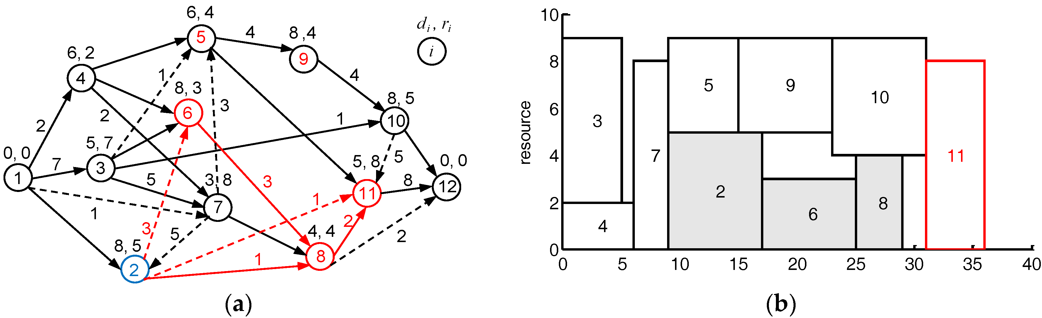
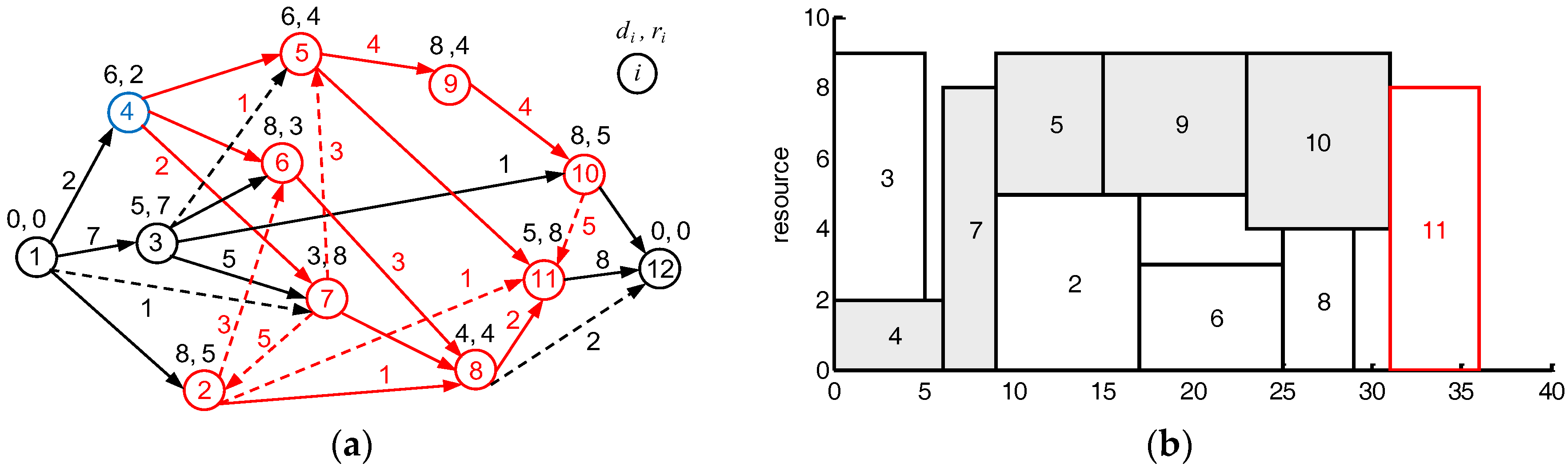
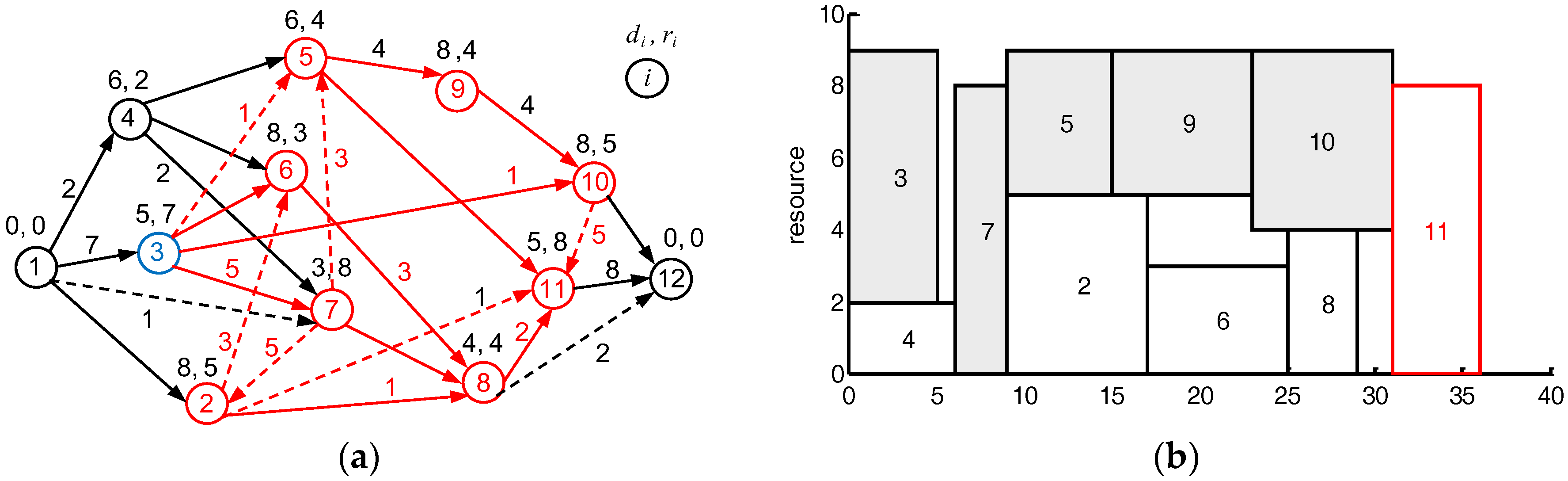
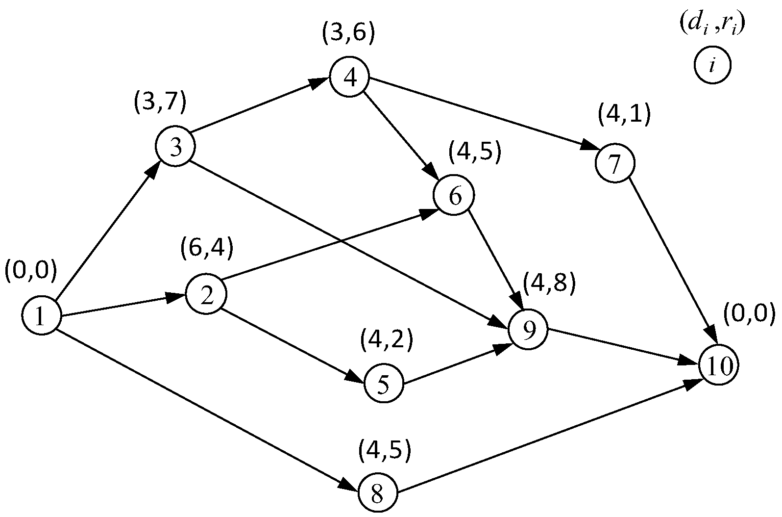
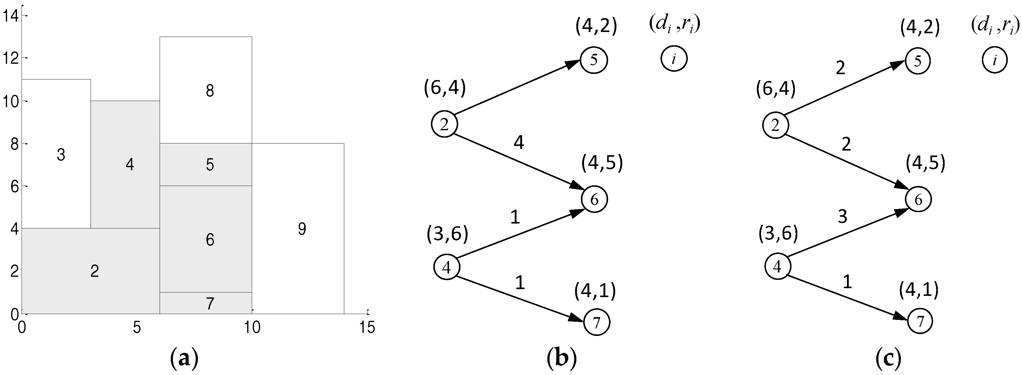
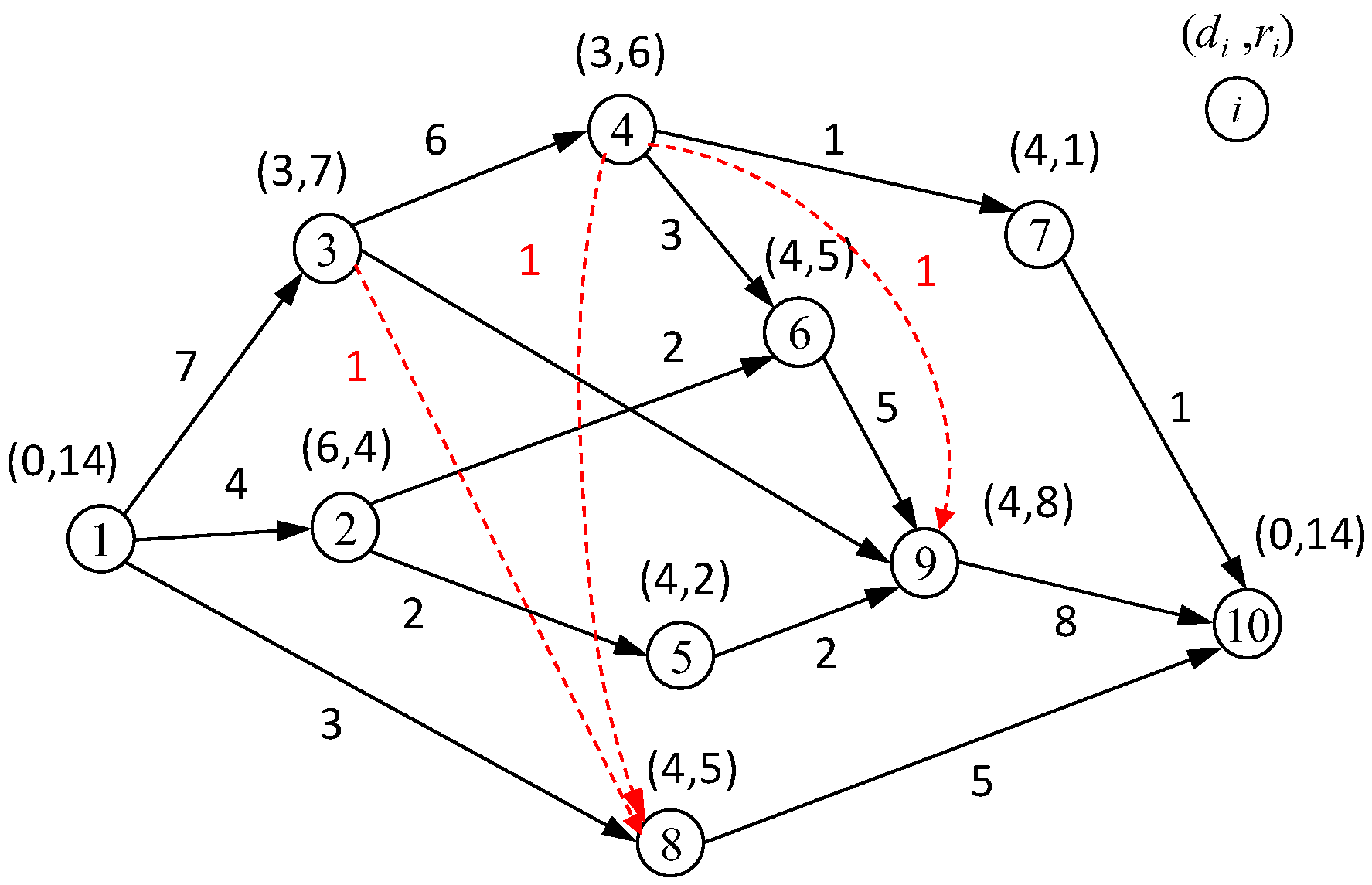
Table 1.
The impact of due date on the robustness when .
| Problem | Robustness Metrics | |||||||||
|---|---|---|---|---|---|---|---|---|---|---|
| RFDFF | STC | UAS | RFDFF | STC | UAS | RFDFF | STC | UAS | ||
| J10 | SP | 0.7449 | 0.7730 | 0.7977 | 0.8117 | 0.8165 | 0.8401 | 0.8968 | 0.8675 | 0.9017 |
| SC | 24.8486 | 24.2272 | 19.2713 | 19.5327 | 18.6960 | 14.0884 | 10.1944 | 14.1227 | 7.1140 | |
| TPCP | 0.6237 | 0.6281 | 0.6261 | 0.7417 | 0.7454 | 0.7416 | 0.8861 | 0.8886 | 0.8864 | |
| APL | 33.1894 | 33.1750 | 33.1526 | 33.1488 | 33.1196 | 33.1661 | 33.1488 | 33.1555 | 33.1587 | |
| SP | 0.6756 | 0.7006 | 0.7104 | 0.7502 | 0.7654 | 0.7709 | 0.8592 | 0.8365 | 0.8546 | |
| J20 | SC | 110.7461 | 103.0997 | 89.5769 | 78.7674 | 72.5052 | 64.5783 | 39.8592 | 48.3712 | 35.2247 |
| TPCP | 0.5080 | 0.5030 | 0.5124 | 0.6698 | 0.6776 | 0.6678 | 0.8830 | 0.8801 | 0.8833 | |
| APL | 54.5441 | 54.5768 | 54.4076 | 54.5441 | 54.3327 | 54.4847 | 54.5441 | 54.4815 | 54.4659 | |
| J30 | SP | 0.6461 | 0.6855 | 0.6622 | 0.7416 | 0.7752 | 0.7465 | 0.8730 | 0.8769 | 0.8581 |
| SC | 205.3720 | 153.3981 | 154.0193 | 145.3222 | 114.7046 | 115.1642 | 72.6573 | 70.4379 | 67.3279 | |
| TPCP | 0.4012 | 0.4149 | 0.3956 | 0.6064 | 0.6151 | 0.6021 | 0.8846 | 0.8857 | 0.8790 | |
| APL | 69.9003 | 69.8646 | 69.8022 | 69.9003 | 69.9853 | 69.9593 | 69.9003 | 69.8613 | 69.9458 | |
Table 2.
The impact of stochastic activity duration on the robustness when .
| Problem | Robustness Metrics | |||||||||
|---|---|---|---|---|---|---|---|---|---|---|
| RFDFF | STC | UAS | RFDFF | STC | UAS | RFDFF | STC | UAS | ||
| J10 | SP | 0.8117 | 0.8165 | 0.8401 | 0.7640 | 0.7590 | 0.7776 | 0.7657 | 0.7585 | 0.7733 |
| SC | 19.5327 | 18.6960 | 14.0884 | 48.2386 | 52.3158 | 43.8052 | 83.7207 | 88.8957 | 79.7710 | |
| TPCP | 0.7417 | 0.7454 | 0.7416 | 0.6152 | 0.6154 | 0.6162 | 0.5977 | 0.5963 | 0.5980 | |
| APL | 33.1488 | 33.1196 | 33.1661 | 34.6062 | 34.6046 | 34.5928 | 36.2456 | 36.2775 | 36.2419 | |
| SP | 0.7502 | 0.7654 | 0.7709 | 0.6967 | 0.6989 | 0.7016 | 0.7010 | 0.7018 | 0.7041 | |
| J20 | SC | 78.7674 | 72.5052 | 64.5783 | 191.2419 | 196.3070 | 181.9613 | 336.7798 | 342.1054 | 330.9924 |
| TPCP | 0.6698 | 0.6776 | 0.6678 | 0.5175 | 0.5158 | 0.5134 | 0.4826 | 0.4850 | 0.4828 | |
| APL | 54.5441 | 54.3327 | 54.4847 | 57.7925 | 57.6623 | 57.7660 | 61.7850 | 61.7099 | 61.8216 | |
| J30 | SP | 0.7416 | 0.7752 | 0.7465 | 0.6970 | 0.7081 | 0.6938 | 0.7019 | 0.7063 | 0.6924 |
| SC | 145.3222 | 114.7046 | 115.1642 | 249.4382 | 240.4390 | 233.2613 | 392.4993 | 397.3236 | 400.9541 | |
| TPCP | 0.6064 | 0.6151 | 0.6021 | 0.4543 | 0.4613 | 0.4607 | 0.4210 | 0.4232 | 0.4190 | |
| APL | 69.9003 | 69.9853 | 69.9593 | 74.0973 | 74.2202 | 73.9554 | 79.7130 | 79.7725 | 79.9574 | |
© 2018 by the authors. Licensee MDPI, Basel, Switzerland. This article is an open access article distributed under the terms and conditions of the Creative Commons Attribution (CC BY) license (http://creativecommons.org/licenses/by/4.0/).
Share and Cite
MDPI and ACS Style
Pang, N.; Su, H.; Shi, Y. Project Robust Scheduling Based on the Scattered Buffer Technology. Appl. Sci. 2018, 8, 541. https://doi.org/10.3390/app8040541
AMA Style
Pang N, Su H, Shi Y. Project Robust Scheduling Based on the Scattered Buffer Technology. Applied Sciences. 2018; 8(4):541. https://doi.org/10.3390/app8040541
Chicago/Turabian StylePang, Nansheng, Huifang Su, and Yingling Shi. 2018. "Project Robust Scheduling Based on the Scattered Buffer Technology" Applied Sciences 8, no. 4: 541. https://doi.org/10.3390/app8040541
Note that from the first issue of 2016, this journal uses article numbers instead of page numbers. See further details here.