Controlling the Spatial Coherence of an Optical Source Using a Spatial Filter


Air Force Institute of Technology, 2950 Hobson Way, Dayton, OH 45433, USA
Appl. Sci. 2018, 8(9), 1465; https://doi.org/10.3390/app8091465
Submission received: 21 July 2018
/
Revised: 10 August 2018
/
Accepted: 22 August 2018
/
Published: 26 August 2018
(This article belongs to the Section Optics and Lasers)
Abstract
:Featured Application
This technique for controlling spatial coherence can be used for beam shaping and reducing scintillation (or fades) in directed energy and free-space optical communication applications.
Abstract
This paper presents the theory for controlling the spectral degree of coherence via spatial filtering. Starting with a quasi-homogeneous partially coherent source, the cross-spectral density function of the field at the output of the spatial filter is found by applying Fourier and statistical optics theory. The key relation obtained from this analysis is a closed-form expression for the filter function in terms of the desired output spectral degree of coherence. This theory is verified with Monte Carlo wave-optics simulations of spatial coherence control and beam shaping for potential use in free-space optical communications and directed energy applications. The simulated results are found to be in good agreement with the developed theory. The technique presented in this paper will be useful in applications where coherence control is advantageous, e.g., directed energy, free-space optical communications, remote sensing, medicine, and manufacturing.
1. Introduction
Following the nomenclature and notation of Emil Wolf [1], a partially coherent source (PCS) is defined by its autocorrelation function, better known as the mutual coherence function (MCF):
where is an instance of a random optical field evaluated at position and time t, * is the complex conjugate, and is the average over the ensemble of U realizations. The first and second moments of many optical sources vary slowly with time such that they can be considered static. This characteristic is referred to as wide-sense stationary and implies that the MCF defined in Equation (1) depends temporally only on the time difference .
The temporal Fourier transform of the MCF is the cross-spectral density (CSD) function:
where is the radian frequency. Letting yields the spectral density (SD), namely,
which is the optical intensity at frequency . Normalizing the CSD produces the spectral degree of coherence (SDoC), i.e.,
which is a measure of the spatial coherence of the source at frequency .
Working with the CSD, as opposed to the MCF, has two significant advantages. The first is the separation of spatial and temporal coherence. In the MCF, time and space are coupled in such a way that determining whether the phenomenon is caused by temporal or spatial coherence can be difficult. On the other hand, the CSD provides a measure of the spatial coherence of an optical source at a certain frequency . In this way, the CSD is much more physical than the MCF, and this physical utility has led to the prediction and subsequent experimental validation of many counter-intuitive optical phenomena, most notably, coherence-induced spectral changes [1,2] and coherence-induced polarization changes [3,4,5].
The second advantage is analytical efficiency. The expression for the propagation of mutual coherence is a complicated four-dimensional (4D) integral over space, where space and time are coupled [6]. The typical approach for dealing with this is to assume that the source is narrowband and quasi-monochromatic. These assumptions simplify the mutual coherence propagation expression significantly; however, they restrict the applicability of the results. On the other hand, the expression for the propagation of CSD—in its most general, paraxial form—is a 4D Fresnel transform [1,5]. In many practical scenarios, the 4D Fresnel transform simplifies to a 4D Fourier transform. The results obtained using these propagation integrals are accurate regardless of the source’s bandwidth.
Wolf’s CSD formalism has led to the understanding and prediction of many optical phenomena. Among these, Wolf and others showed that a spatially partially coherent beam (PCB) can be highly directional similar to a laser [1,7,8,9]. Other research soon followed, showing that the reduced spatial coherence of PCBs makes them less susceptible to scintillation or speckle [5,10,11,12,13]. These two discoveries have motivated much of the recent PCS research because high directionality and speckle/scintillation resistance are ideal source characteristics for directed energy, free-space optical communications (FSOC), medical, and numerous other applications.
Because of their many potential uses, the literature is replete with techniques to synthesize sources with controllable spatial coherence. A survey of the literature reveals two general approaches for generating PCBs. The first starts with a spatially coherent source, commonly a laser, and “spoils” the coherence by randomizing the wavefront. This is accomplished using spatial light modulators (SLMs) or rotating ground glass diffusers (GGDs) [5,14,15]. The second approach starts with a spatially incoherent source, an LED for instance, and exploits the Van Cittert–Zernike theorem (VCZT) or uses spatial-frequency filters (typically referred to as just spatial filters) to synthesize the desired source [16,17,18,19,20]. Hybrid approaches have also been developed [11,12,21].
The “coherent” and “incoherent” PCS synthesis methods discussed above have pros and cons that make one more suitable for a specific application than the other. FSOC is a good example and will be the focus of the remainder of this paper because of the author’s research interests. In FSOC, the source’s wavefront cycling rate, i.e., the rate at which the source produces statistically independent wavefronts, must be at least 10–100 times larger than the communication modulation frequency. This is so the detector integrates many independent intensity realizations per digital bit to reduce scintillation caused by atmospheric turbulence between the transmitter and receiver. Considering that FSOC data rates are gigabits to potentially terabits per second and SLM frame rates and GGD rotation rates are optimistically 10 kHz, spoiling the coherence of a laser source is not a realistic option.
On the other hand, the wavefront cycling rate of a spatially incoherent source (e.g., an LED, thermal source, et cetera) is determined by the physics of how the source generates light (for the aforementioned sources, the physical mechanism is spontaneous emission) and is ultimately related to the source’s bandwidth [6]. The bandwidths of such sources applicable to FSOC vary from a couple THz to 10 s of THz. Even for sources at the low end of this range, the wavefront cycles so quickly that 100 gigabit per second data rates are possible. Because of this, the incoherent option is the only viable approach for FSOC applications.
Of the two incoherent techniques, i.e., VCZT and spatial filtering, the latter has many advantages including simplicity and compactness. Surprisingly, despite these advantages and its common use in optical Fourier processing [22], the spatial filtering of a partially coherent source (PCS) has been discussed in relatively few papers [19,20,23,24]. These references, after presenting the requisite Fourier and statistical optics theory, generally focus on specific PCSs, e.g., Gaussian Schell model [1,5] or incoherent sources. Simple, physical, “engineering” expressions for the PCS at the filter output, or directions for designing/choosing a filter to produce a desired beam are not presented.
The goal of this paper is to derive these expressions and demonstrate their use. In the next section, starting with a stochastic source field, the field at the output of a general spatial filter is derived. Taking the autocorrelation of the output field and assuming that the source field can be modeled as a quasi-homogeneous source [1,6] yields closed-form, approximate expressions for the output SD and SDoC. Inverting the SDoC expression produces a function for the filter in terms of the desired output SDoC. Lastly, Section 3 validates these theoretical expressions and demonstrates how to use them to control coherence and beam shape via Monte Carlo wave-optics simulations.
2. Materials and Methods
2.1. Fourier and Statistical Optics Theory
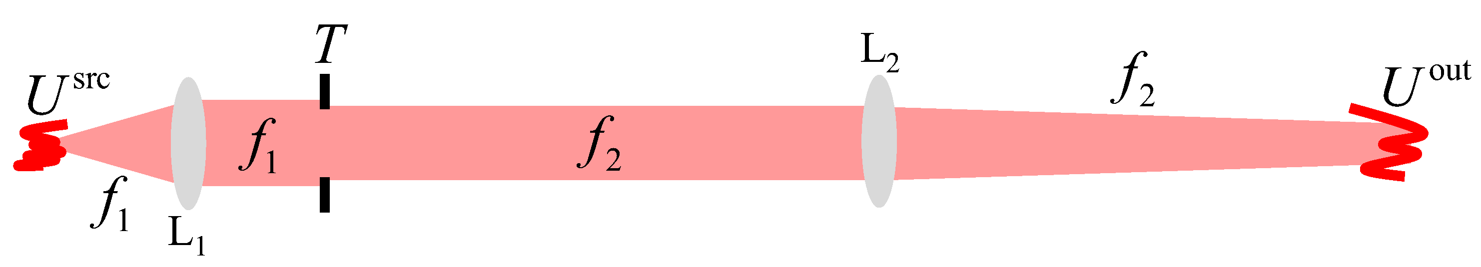
The spatial filter geometry is shown in Figure 1. This simple geometry depicts a random field passing through a two-lens system. The source plane is one focal length in front of . The field passes through and then a complex amplitude filter T placed at the rear focus of . The location of T also corresponds to the front focal plane of . The field then transits before finally being observed in ’s rear focal plane.
Assuming that is large enough in diameter to collect all the light emitted from the source, the field in ’s focal plane, right before T, is
where is the observation vector, is the source vector, , and is the wavelength [22]. The random source field is assumed to be a sample function drawn from a wide-sense stationary random process (the dependence of on radian frequency is assumed and suppressed), and is the spatial Fourier transform of :
where is the spatial frequency vector.
The field immediately to the right of the complex amplitude filter is
Lastly, assuming that is large enough to capture all the light that passes through T, the field at the output of the spatial filter is [22]
The output field given in Equation (8) is for a single realization of the random source field . Taking the autocorrelation of produces
where is the output CSD function [1,5] and is the Fourier transform of the source CSD function. It is quite easy to show that an equivalent and more physical expression for is
where is the magnification. This expression states that is the scaled convolution of with the Fourier transform of the CSD function of T. In arriving at Equations (9) and (10), no assumptions have been made about the spatial statistics of ; thus, they are accurate for a source of any state of coherence.
To make further progress, an analytical form for is needed. Because of its use in FSOC research, the physical source modeled here is the output of a multimode fiber (MMF) excited by a “broadband” (1–2 THz) laser [25,26,27]. This source can be approximated by a quasi-homogeneous CSD function [1,5,6], which takes the form
where is the source’s SD, is the source’s SDoC, and is a “slow function” (varies slowly) compared to .
Taking the Fourier transform of Equation (11) and substituting the resulting expression into Equation (9) produces
Making the variable substitutions and and simplifying, yields
Now, assuming is a very narrow function of (much narrower than T), Equation (13) can be approximated as
Note that this assumption is equivalent to assuming that the integrand of Equation (12), without the Fourier kernel, is another quasi-homogeneous source. Evaluating the above Fourier integrals produces
The output SD and SDoC are
Note that the output SD (physically, the source shape) is a magnified version of , and the output SDoC is a magnified and filtered version of .
Although expressions for and have been derived, an equation for T in terms of (i.e., what T yields a given ) is most useful. Starting with the above expression for given in Equation (16) and assuming that is a slow function compared to T (this is actually a consequence of assuming a quasi-homogeneous form) produces
Letting for convenience and substituting into both the numerator and denominator integrals simplifies Equation (17) to
Applying the Fourier transform defined in Equation (6) to both sides of Equation (18) produces the desired result:
This expression states that the spatial power spectrum of the output field (the Fourier transform of ) is proportional to the magnitude squared of T rotated 180. The proportionality constant is there to normalize the area under the power spectrum; it is inconsequential in practice. The above interpretation of Equation (19) leads to the following steps for finding T:
- Choose the desired output SDoC .
- Compute the spatial Fourier transform of to find .
- Take the square root of to find the magnitude of T.
- Normalize T such that .
- Rotate T 180.
It should be stated that Equations (16) and (19) are accurate if the following three conditions hold:
- The diameters of lenses and are large enough to collect all the light emitted from the source and the light that passes through the spatial filter T, respectively.
- The random source field is well approximated by a CSD function with a quasi-homogeneous form.
- is a fast function (narrow function) compared to T.
The first item is easily met in practice by using ray tracing and other standard optical design techniques. The second criterion is true for “spatially incoherent” sources such as LEDs or, applicable here, the light emitted from a broadband-laser-excited MMF. The third condition is the hardest to satisfy in practice. The effects of violating this condition are shown in Section 3.1.
Because of the assumptions that underpin the analysis (enumerated above), Equations (16) and (19) are approximations of the output PCS moments. Recall that the goal here was to find simple, physical, “engineering” expressions that could be used to design a spatial filter that would produce a desired PCS. Equations (16) and (19) achieve that objective.
2.2. Simulation Details
The purpose of the Monte Carlo wave-optics simulations is to validate the above analysis and to demonstrate how to apply it, specifically Equations (16) and (19), to generate a desired PCS. Before proceeding to the results, a brief discussion of the set-up is warranted.
To simulate the output of a MMF fed by a broadband laser [25,26,27], took the form
where is the circle function defined by Goodman [22], , and is a first-order Bessel function of the first kind. The fiber’s core diameter and numerical aperture were and , respectively. The simulated wavelength was . Instances of were synthesized from using the method described in [28].
The focal lengths of the lenses comprising the spatial filter were and (see Figure 1). The source, focal, and output planes were discretized using 512 points per side with grid spacings equal to 0.8203 m, 0.1512 mm, and 4.102 m, respectively. All propagations were performed using fast Fourier transforms [29].
The desired, output SDoC (after filtering) was
where . This SDoC was chosen to show that a source with a rotationally invariant CSD function (see Equation (20)) can be transformed (via filtering) into one with different, specified x and y correlation lengths. The required T to synthesize a source with this SDoC was determined using the five steps enumerated above. Figure 2a shows this T.
The simulated output SD and were computed from 2000 propagated instances of . These results were then compared to the theoretical predictions given in Equation (16). All simulations were performed using MATLAB® version R2017a (The MathWorks, Inc., Natick, MA, USA); the scripts (.m files) are included as Supplementary Materials.
3. Results and Discussion
3.1. Spatial Coherence Control
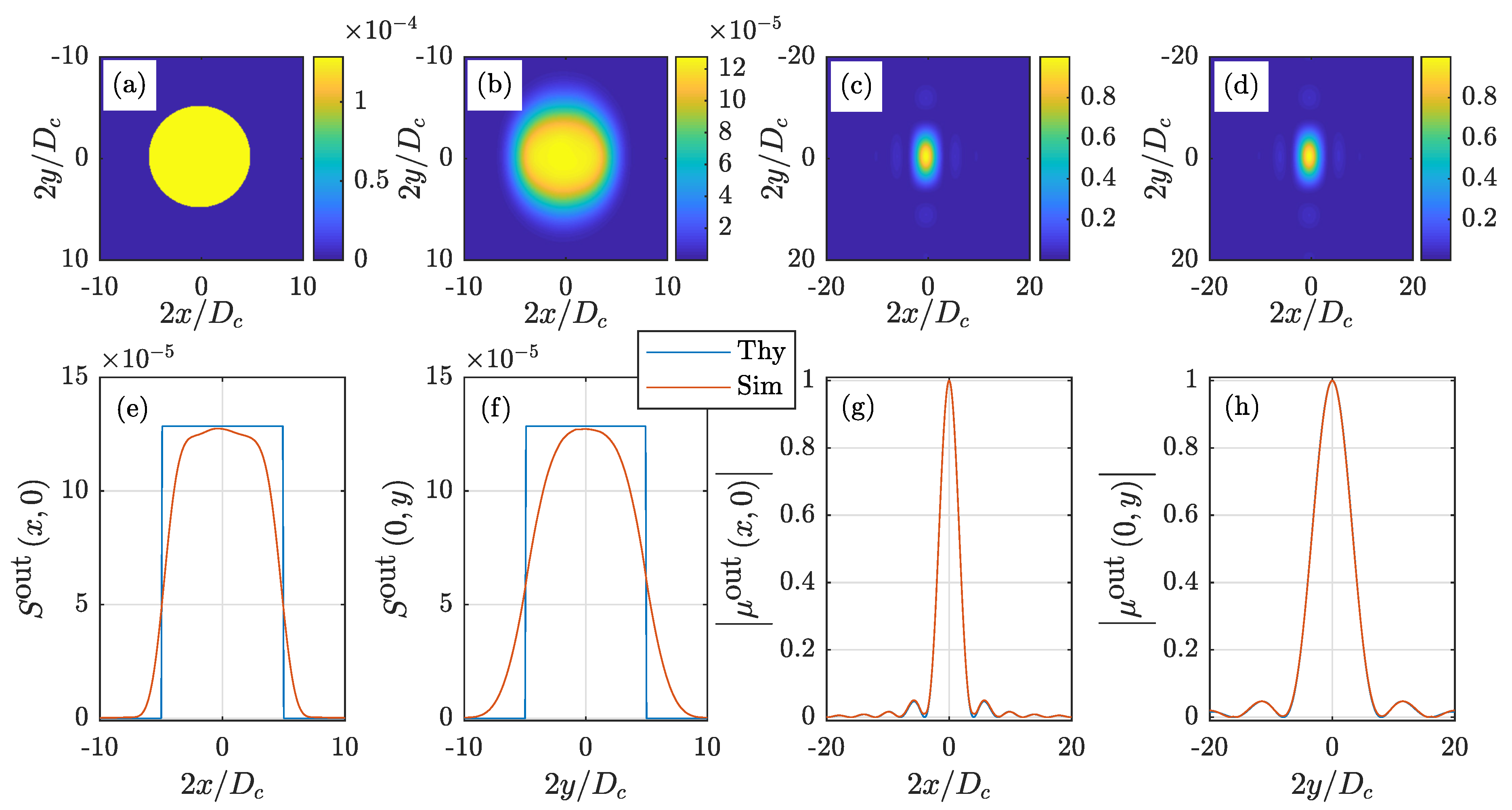
Figure 3 shows the simulation results. Figure 3a,b shows the theoretical and simulated SDs ( obtained from Equation (16) and ); Figure 3c,d shows the theoretical and simulated SDoCs ( given in Equation (21) and ); Figure 3e,f shows the and slices through and ; and Figure 3g,h shows the and slices through and .
The and results noticeably disagree. This occurs because is not a fast function compared to T, viz., Criterion 3 is violated. Recall that this assumption was made in going from Equation (13) to Equation (14). The width of in the y direction is larger than in the x direction (see Equation (21)). The Fourier transform relationship between T and means T has complementary widths to , i.e., T is wider in the x direction than in the y direction. This -T relationship explains why compares better to in Figure 3e than in Figure 3f.
Although and disagree, the objective here is to control spatial coherence as measured by the SDoC. Figure 3c,d,g,h shows these results. Clearly, the effects of violating Criterion 3 are generally limited to the output SD because the agreement between and is excellent. These results validate the PCS spatial filtering method presented here.
3.2. Beam Shaping
The results presented in Figure 3 demonstrated that the output SDoC could be precisely controlled by the proper choice of T. A related application where the Section 2.1 analysis can also be applied is beam shaping.
The goal in beam shaping is to produce a beam with a desired SD at a desired location—typically, at the focus of a lens or, equivalently, in the far zone of the source. Referring back to Equation (15), propagating to the far field, and setting yields the far-zone SD:
Note that the source takes the shape of the absolute square of the filter—magnified and rotated 180—in the far field. This can be exploited to produce beams of any desired shape.
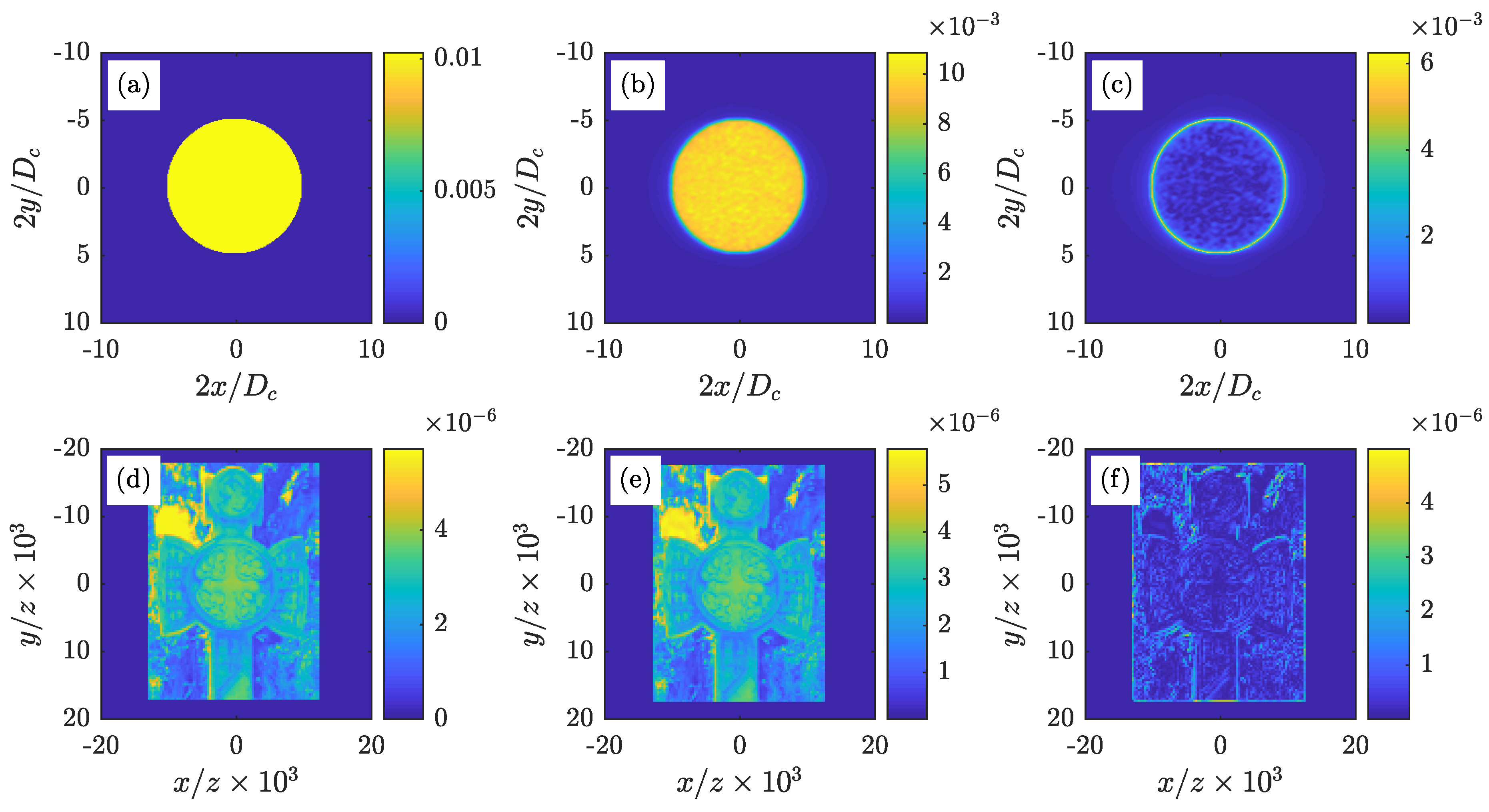
As an example, Figure 4 shows the results of a beam shaping simulation. The source (see Equation (20)) and set-up were identical to that described in Section 2.2, only T was changed to produce a beam with a more complex shape. Figure 2b shows this T.
Figure 4a,b shows (obtained from Equation (16)) and , respectively. By design, these SDs should look very similar to those in Figure 3a,b—the differences are due to the different T. Figure 4c shows the absolute value of the pixel-by-pixel difference of Figure 4a,b.
Figure 4d,e shows the theoretical and simulated far-zone SDs, obtained from Equation (22) and , respectively. The theoretical far-zone SD is the desired beam shape. was computed from 2000 far-zone propagated instances of (these propagations were simulated using fast Fourier transforms [29]), which were obtained from 2000 instances of , synthesized in the manner described in [28]. Similarly, Figure 4c,f shows the absolute value of the pixel-by-pixel difference of Figure 4d,e.
The agreement between the simulated and theoretical SDs is excellent. These results further validate the analysis presented in Section 2.1.
If one were to physically generate this source, it would start as partially coherent light emitted from a MMF. It would exit the spatial filter as a circular flat-topped beam, as shown in Figure 4a,b. As the beam propagated away from the spatial filter output plane, it would morph into the Celtic cross image shown in Figure 4d,e.
4. Conclusions
The control of an optical source’s SDoC via spatial filtering was demonstrated. Starting with a quasi-homogeneous random field, the optical field at the output of a general spatial filter was derived. Taking moments of the stochastic output field yielded closed-form expressions for the output SD and SDoC. The key relation which resulted from this analysis was a closed-form expression for the filter function T in terms of the desired SDoC.
The analytical SD and SDoC equations derived in Section 2.1 were verified by Monte Carlo analysis. First, the T required to produce a specified SDoC was found using the steps developed and discussed in Section 2.1. Then, simulating a source used in FSOC research (namely, the stochastic field emitted from a MMF excited by a broadband laser source) and a simple spatial filter containing T, the output SD and SDoC were computed from many independent realizations of the source field. Lastly, the simulated output SD and SDoC were compared to the theoretical predictions. The agreement between the two was generally good with some discrepancies between the simulated and theoretical SDs. The reason for these differences was discussed.
In addition, a beam shaping simulation was also performed to demonstrate another use of coherence control via spatial filtering. Using the analytical relations derived in Section 2.1, an approximate expression for the desired far-zone SD, in terms of the filter function T, was derived. This equation was used to find the T required to synthesize a beam with a complex shape. The simulated results were in excellent agreement with the derived, analytical SDs.
The spatial filtering technique presented in this paper has many advantages over other PCS synthesis methods. First and foremost among them is speed. As discussed in the Introduction, the wavefront cycling rate for this method can be 10s of THz, which is 10 times faster than SLM- or GGD-based approaches. When compared against other incoherent synthesis techniques (e.g., VCZT), spatial filtering is simpler to implement. As demonstrated in Section 3, changing the output field SDoC requires only a filter change. These pros make PCS spatial filtering useful in any application where coherence control is advantageous. These include, but are not limited to, FSOC, directed energy, medicine, manufacturing, and remote sensing.
Supplementary Materials
Supplementary materials can be found at https://www.mdpi.com/2076-3417/8/9/1465/s1.
Author Contributions
M.W.H. performed the works of conceptualization, formal analysis, methodology, software, validation, visualization, writing—original draft, and writing—reviewing & editing.
Funding
This research received no external funding.
Acknowledgments
The views expressed in this paper are those of the authors and do not reflect the official policy or position of the US Air Force, the Department of Defense, or the US government.
Conflicts of Interest
The author declares no conflicts of interest.
References
- Mandel, L.; Wolf, E. Optical Coherence and Quantum Optics; Cambridge University: New York, NY, USA, 1995. [Google Scholar]
- Wolf, E.; James, D.F.V. Correlation-induced spectral changes. Rep. Prog. Phys. 1996, 59, 771–818. [Google Scholar] [CrossRef]
- James, D.F.V. Change of polarization of light beams on propagation in free space. J. Opt. Soc. Am. A 1994, 11, 1641–1643. [Google Scholar] [CrossRef]
- Wolf, E. Introduction to the Theory of Coherence and Polarization of Light; Cambridge University: New York, NY, USA, 2007. [Google Scholar]
- Korotkova, O. Random Light Beams: Theory and Applications; CRC: Boca Raton, FL, USA, 2014. [Google Scholar]
- Goodman, J.W. Statistical Optics, 2nd ed.; Wiley: Hoboken, NJ, USA, 2015. [Google Scholar]
- Collett, E.; Wolf, E. Is complete spatial coherence necessary for the generation of highly directional light beams? Opt. Lett. 1978, 2, 27–29. [Google Scholar] [CrossRef] [PubMed]
- Wolf, E.; Collett, E. Partially coherent sources which produce the same far-field intensity distribution as a laser. Opt. Commun. 1978, 25, 293–296. [Google Scholar] [CrossRef]
- Gori, F.; Palma, C. Partially coherent sources which give rise to highly directional light beams. Opt. Commun. 1978, 27, 185–188. [Google Scholar] [CrossRef]
- Gbur, G. Partially coherent beam propagation in atmospheric turbulence. J. Opt. Soc. Am. A 2014, 31, 2038–2045. [Google Scholar] [CrossRef] [PubMed]
- Cai, Y.; Chen, Y.; Yu, J.; Liu, X.; Liu, L. Generation of partially coherent beams. Prog. Opt. 2017, 62, 157–223. [Google Scholar] [CrossRef]
- Cai, Y.; Chen, Y.; Wang, F. Generation and propagation of partially coherent beams with nonconventional correlation functions: A review. J. Opt. Soc. Am. A 2014, 31, 2083–2096. [Google Scholar] [CrossRef] [PubMed]
- Drexler, K.R.; Roggemann, M.C.; Voelz, D.G. Use of a partially coherent transmitter beam to improve the statistics of received power in a free-space optical communication system: Theory and experimental results. Opt. Eng. 2011, 50, 025002. [Google Scholar] [CrossRef]
- Hyde, M.W.; Basu, S.; Voelz, D.G.; Xiao, X. Experimentally generating any desired partially coherent Schell-model source using phase-only control. J. Appl. Phys. 2015, 118, 093102. [Google Scholar] [CrossRef] [Green Version]
- Hyde, M.W.; Bose-Pillai, S.R.; Wood, R.A. Synthesis of non-uniformly correlated partially coherent sources using a deformable mirror. Appl. Phys. Lett. 2017, 111, 101106. [Google Scholar] [CrossRef]
- Santarsiero, M.; Borghi, R.; Ramírez-Sánchez, V. Synthesis of electromagnetic Schell-model sources. J. Opt. Soc. Am. A 2009, 26, 1437–1443. [Google Scholar] [CrossRef]
- Santarsiero, M.; Martínez-Herrero, R.; Maluenda, D.; de Sande, J.C.G.; Piquero, G.; Gori, F. Partially coherent sources with circular coherence. Opt. Lett. 2017, 42, 1512–1515. [Google Scholar] [CrossRef] [PubMed]
- Ostrovsky, A.S.; Martínez-Niconoff, G.; Martínez-Vara, P.; Olvera-Santamaría, M.A. The van Cittert-Zernike theorem for electromagnetic fields. Opt. Express 2009, 17, 1746–1752. [Google Scholar] [CrossRef] [PubMed]
- Visser, T.D.; Agrawal, G.P.; Milonni, P.W. Fourier processing with partially coherent fields. Opt. Lett. 2017, 42, 4600–4602. [Google Scholar] [CrossRef] [PubMed]
- Wu, T.; Liang, C.; Wang, F.; Cai, Y. Shaping the intensity and degree of coherence of a partially coherent beam by a 4f optical system with an amplitude filter. J. Opt. 2017, 19, 124010. [Google Scholar] [CrossRef]
- Gori, F.; Santarsiero, M. Devising genuine spatial correlation functions. Opt. Lett. 2007, 32, 3531–3533. [Google Scholar] [CrossRef] [PubMed]
- Goodman, J.W. Introduction to Fourier Optics, 3rd ed.; Roberts & Company: Englewood, CO, USA, 2005. [Google Scholar]
- Indebetouw, G. Synthesis of polychromatic light sources with arbitrary degrees of coherence: Some experiments. J. Mod. Opt. 1989, 36, 251–259. [Google Scholar] [CrossRef]
- Mendlovic, D.; Shabtay, G.; Lohmann, A.W. Synthesis of spatial coherence. Opt. Lett. 1999, 24, 361–363. [Google Scholar] [CrossRef] [PubMed]
- Pask, C.; Snyder, A.W. The Van Cittert-Zernike theorem for optical fibres. Opt. Commun. 1973, 9, 95–97. [Google Scholar] [CrossRef]
- Efimov, A. Spatial coherence at the output of multimode optical fibers. Opt. Express 2014, 22, 15577–15588. [Google Scholar] [CrossRef] [PubMed]
- Fathy, A.; Sabry, Y.M.; Khalil, D.A. Quasi-homogeneous partial coherent source modeling of multimode optical fiber output using the elementary source method. J. Opt. 2017, 19, 105605. [Google Scholar] [CrossRef] [Green Version]
- Voelz, D.; Xiao, X.; Korotkova, O. Numerical modeling of Schell-model beams with arbitrary far-field patterns. Opt. Lett. 2015, 40, 352–355. [Google Scholar] [CrossRef] [PubMed]
- Schmidt, J.D. Numerical Simulation of Optical Wave Propagation with Examples in MATLAB; SPIE Press: Bellingham, WA, USA, 2010. [Google Scholar]
Figure 1.
Spatial filter geometry.

Figure 2.
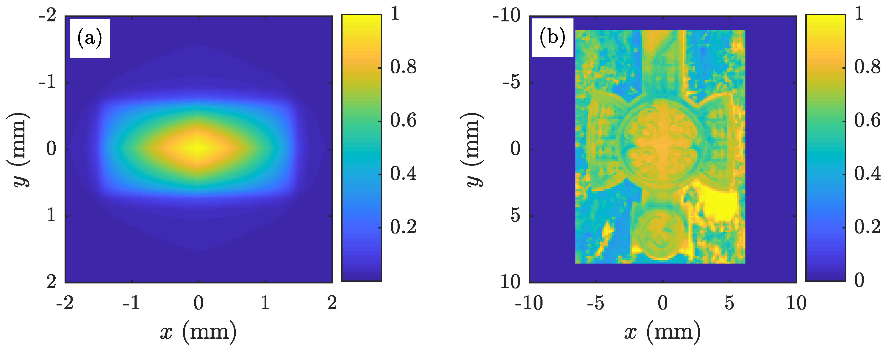
Spatial filter T images: (a) spatial coherence control simulation (Section 3.1); and (b) beam shaping simulation (Section 3.2).
Figure 2.
Spatial filter T images: (a) spatial coherence control simulation (Section 3.1); and (b) beam shaping simulation (Section 3.2).

Figure 3.
Simulation results demonstrating coherence control using a spatial filter: (a) obtained from Equation (16); (b) ; (c) given in Equation (21); (d) ; (e) slices of and ; (f) slices of and ; (g) slices of and ; and (h) slices of and .


© 2018 by the author. Licensee MDPI, Basel, Switzerland. This article is an open access article distributed under the terms and conditions of the Creative Commons Attribution (CC BY) license (http://creativecommons.org/licenses/by/4.0/).
Share and Cite
MDPI and ACS Style
Hyde, M.W., IV. Controlling the Spatial Coherence of an Optical Source Using a Spatial Filter. Appl. Sci. 2018, 8, 1465. https://doi.org/10.3390/app8091465
AMA Style
Hyde MW IV. Controlling the Spatial Coherence of an Optical Source Using a Spatial Filter. Applied Sciences. 2018; 8(9):1465. https://doi.org/10.3390/app8091465
Chicago/Turabian StyleHyde, Milo W., IV. 2018. "Controlling the Spatial Coherence of an Optical Source Using a Spatial Filter" Applied Sciences 8, no. 9: 1465. https://doi.org/10.3390/app8091465
Note that from the first issue of 2016, this journal uses article numbers instead of page numbers. See further details here.