Halo-Free Multi-Exposure Image Fusion Based on Sparse Representation of Gradient Features
by
Hua Shao
1,2, 
Gangyi Jiang
1,3,
Mei Yu
1,3,*,
Yang Song
1,
Hao Jiang
1,
Zongju Peng
1 and
Feng Chen
1 1
Faculty of Information Science and Engineering, Ningbo University, Ningbo 315211, China
2
Faculty of Information and Intelligent Engineering, Ningbo City College of Vocational Technology, Ningbo 315100, China
3
National Key Lab of Software New Technology, Nanjing University, Nanjing 210093, China
*
Author to whom correspondence should be addressed.
Appl. Sci. 2018, 8(9), 1543; https://doi.org/10.3390/app8091543
Submission received: 6 July 2018
/
Revised: 26 August 2018
/
Accepted: 29 August 2018
/
Published: 3 September 2018
(This article belongs to the Section Optics and Lasers)
Abstract
:Due to sharp changes in local brightness in high dynamic range scenes, fused images obtained by the traditional multi-exposure fusion methods usually have an unnatural appearance resulting from halo artifacts. In this paper, we propose a halo-free multi-exposure fusion method based on sparse representation of gradient features for high dynamic range imaging. First, we analyze the cause of halo artifacts. Since the range of local brightness changes in high dynamic scenes may be far wider than the dynamic range of an ordinary camera, there are some invalid, large-amplitude gradients in the multi-exposure source images, so halo artifacts are produced in the fused image. Subsequently, by analyzing the significance of the local sparse coefficient in a luminance gradient map, we construct a local gradient sparse descriptor to extract local details of source images. Then, as an activity level measurement in the fusion method, the local gradient sparse descriptor is used to extract image features and remove halo artifacts when the source images have sharp local changes in brightness. Experimental results show that the proposed method obtains state-of-the-art performance in subjective and objective evaluation, particularly in terms of effectively eliminating halo artifacts.
1. Introduction
There is abundant information about brightness and color in real natural scenes, and the dynamic range is very wide. Therefore, high dynamic range (HDR) images, which can truly represent natural scenes, are widely used in digital photography, aerospace, satellite meteorology, medical treatment, and military industries [1,2,3].
The HDR imaging technology can be divided into two categories. The first is the hardware-based method [4,5], which utilizes HDR devices to capture real natural scenes. However, these devices are too expensive to be popular with the public. The second uses software-based technology to obtain HDR images [6]. The notion of this category is that real natural scenes can be captured with a stack of low dynamic range (LDR) images with different exposures, and an HDR image can be obtained by using the camera response function [7,8]. Then, tone mapping technology [9,10,11] is used to reduce the dynamic range of the HDR image for display on the common device. However, the quality of the reconstructed HDR image depends heavily on the related exposure settings (e.g., exposure time and exposure value), which are often unknown to the user. Therefore, software-based HDR imaging technology through multi-exposure fusion [12,13,14] has attracted increasing amounts of attention. This technology can directly obtain greater information and produce a more perceptually appealing composite LDR image, reflecting natural scenes more closely. Furthermore, the result of a multi-exposure fusion can be directly presented on the LDR displays.
In recent years, many scholars have performed in-depth studies on multi-exposure fusion. Mertens et al. [15] proposed a multi-exposure fusion method based on weight maps, the factors of which are comprised of three quality measures (i.e., contrast, saturation, and exposure quality at the pixel level). Moreover, the multi-resolution approach, based on Laplacian pyramids, was also applied to pursue better human visual perception. However, this method placed too much emphasis on contrast. Thus, the details of brighter and darker regions were lost in the fused image. Vonikakis et al. [16] evaluated the exposure quality of pixels in the source images via illumination estimation filtering and then realized multi-exposure image fusion. Zhang et al. [17] achieved the multi-exposure fused image with gradient information, which can effectively preserve texture details. Li et al. [18] decomposed a number of multi-exposure source images into a detailed layer, containing small-scale details, and a base layer, containing large-scale intensity variations. Then, they used spatial consistency to fuse the basic and detailed layers. Shen et al. [19] proposed a multi-exposure fusion method, based on an improved pyramid, to preserve detail information. Liu et al. [12] introduced a dense scale invariant feature transform (SIFT) descriptor into image fusion to extract local details from multi-exposure source images. Ma et al. [13] proposed a multi-exposure fusion method, based on an effective structural path decomposition approach, which took account of the local and global characteristics of the source images and obtained better fused image quality. Prabhakar et al. [20] proposed an unsupervised deep learning framework for multi-exposure fusion (MEF), utilizing a no-reference quality metric as the loss function, which obtained excellent fusion results. On the basis of Ma et al. [13], Ma et al. [14] then proposed a multi-exposure fusion method by optimizing the color multi-exposure fusion structural similarity (MEF-SSIMc) index. However, the above fused methods did not consider that there were halo artifacts in the multi-exposure fused image. These halo artifacts always occur in the region of sharp local brightness changes, severely reducing the perceptual appeal.
Additionally, the theory of sparse representation shows that the linear combination of a “few” atoms from an over-complete dictionary can effectively describe the salient features of objects [21,22,23]. Thus, it has been widely used for image processing. Yang et al. [24] introduced sparse representation into image fusion. With their method, source images were divided into small patches and transformed into vectors via lexicographic ordering. They then realized sparse representation using an over-complete dictionary. Liu et al. [25] combined multi-scale transformation and sparse representation to constitute a general image fusion framework, which presented more details in the fused images. However, these works mainly focused on multi-focus and multi-modal fusion, and because they did not consider the characteristics of multi-exposure source images, they are still not appropriate for multi-exposure image fusion.
In this paper, we propose a halo-free multi-exposure fusion method based on sparse representation of gradient features. In our method, the local gradient sparse descriptor, obtained from a gradient map through sparse representation, is used for both local detail extraction and halo artifact removal. The main contributions of this paper can be summarized in the following three points:
- (1)
- By analyzing characteristics of the luminance gradient in multi-exposure source images, the cause of halo artifacts in the fused image is discussed. Because the local brightness changes in HDR scenes are violent, they can far exceed the dynamic range of a single photograph. Thus, the halo artifacts in the fused image are generated by the invalid large-amplitude gradients in the source images.
- (2)
- By calculating the l1-norm of the sparse coefficients in the luminance gradient map, we obtain the local gradient sparse descriptor as the feature of the images. This descriptor can effectively extract local details of source images.
- (3)
- A new multi-exposure fusion method based on the local gradient sparse descriptor is proposed, which can achieve a halo-free fused image by restraining the invalid large-amplitude gradients. Meanwhile, the fused image of the proposed method is not recovered by the over-complete dictionary, which effectively improves the fusion efficiency.
The remainder of this paper is organized as follows: In Section 2, we analyze the cause of halo artifacts in the multi-exposure fused images; Section 3 presents the proposed halo-free fusion method; the experimental results and discussions are described in Section 4; and finally, Section 5 concludes the paper.
2. Cause of Halo Artifacts in Fused Images
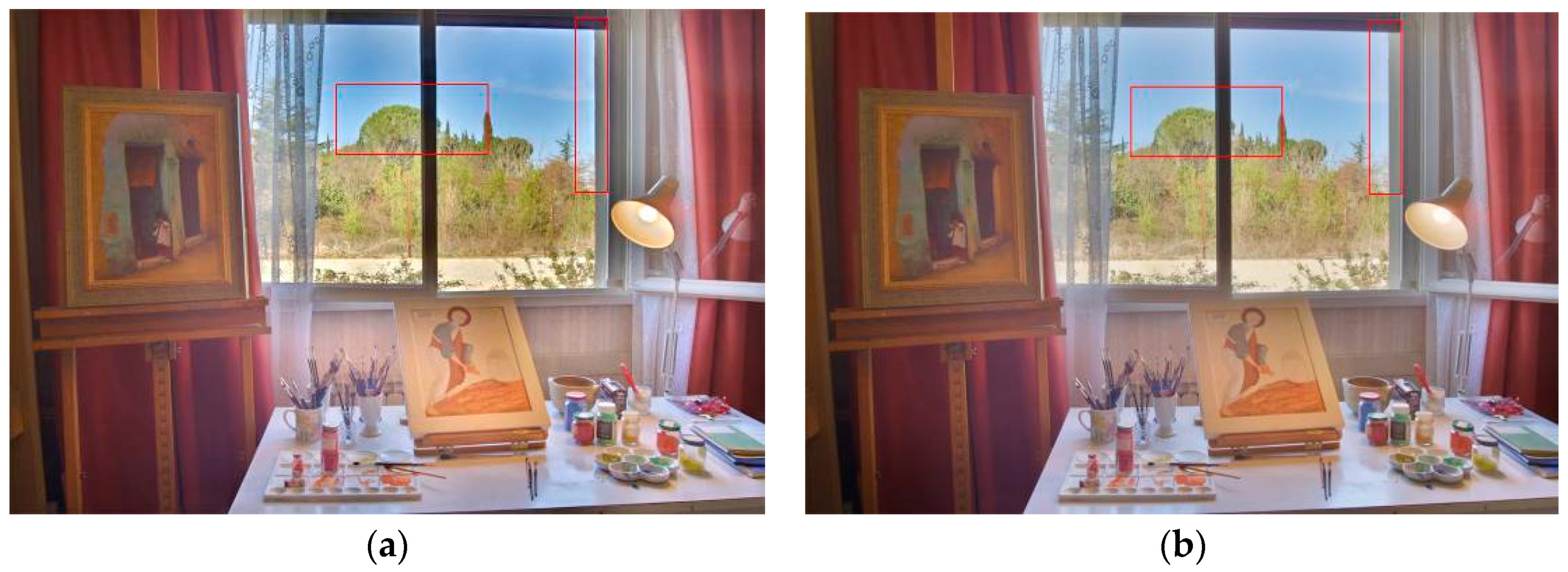
In HDR natural scenes, there is not only abundant information about brightness and color, but also plenty of sharp local brightness changes. In the process of multi-exposure fusion, if those sharp brightness changes cannot be fully considered, the halo artifacts will appear in the fused images. As seen in Figure 1a, which shows the fused result of Li et al. [18], halo artifacts have occurred in the sky outside the windows. By contrast, the sharp local brightness changes are fully considered in the proposed method. Thus, the fused image is more consistent with human visual perception through the removal of halo artifacts, as shown in Figure 1b.
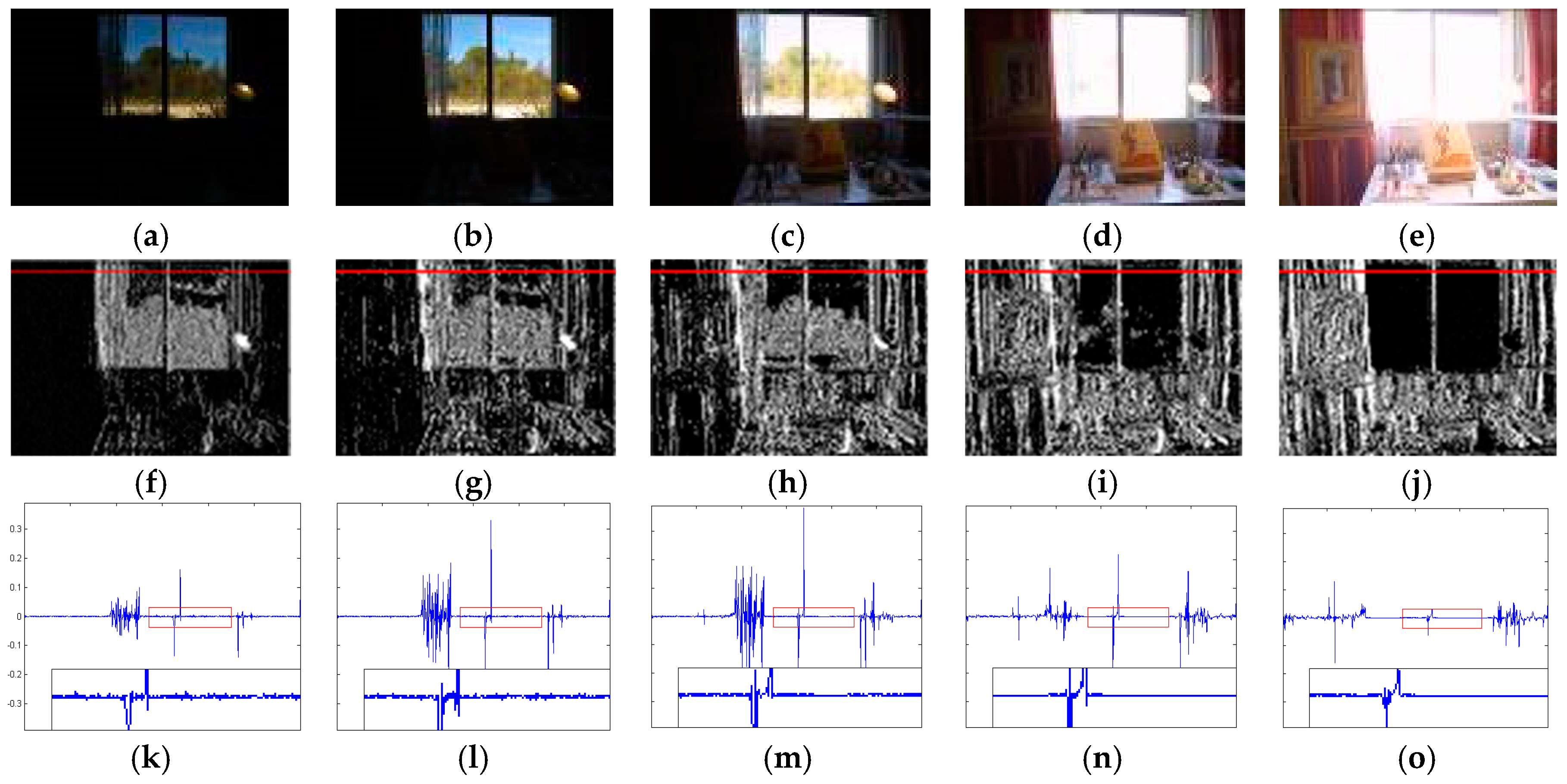
The cause of these halo artifacts are revealed in Figure 2. In the multi-exposure source images of Figure 2a–c, the exposure of the scenery outside the window is increasing until over-exposure, while the brightness contrast increases step-by-step between indoors and outdoors. In the local luminance gradient amplitude of Figure 2k–o, the maximal gradient is found in Figure 2m. However, the region around the maximal gradient in the corresponding source image in Figure 2c is over-exposed and unsuitable for the fused image. However, in the same position of Figure 2a,b, the well-exposed region can be found, which are more suitable for the fused image than that of Figure 2c. Therefore, the maximal gradient existing in Figure 2m is an invalid gradient and the primary cause of halo artifacts in the fused image. The reason for this phenomenon is that a single photograph has very limited dynamic range, compared to real HDR scenes. Thus, the invalid large-amplitude gradients occur in the multi-exposure source images. If these invalid gradients cannot be suppressed, halo artifacts are inevitable in the fused image.
In most multi-exposure image fusion methods, the image features, such as contrast and saliency, are used as weight coefficients for image fusion, except for the gradient. However, these image features have more or less a direct connection with the gradient, which leads to halo artifacts of varying degrees in the fusion results. In the method by Mertens et al. [15], a Laplacian filter was applied to the grayscale version of each multi-exposure image to yield a simple indicator, C, for contrast. This indicator C was then used as one of the weight coefficients for image fusion. Generally, pixels with larger contrast always have larger gradients, so the pixels with invalid large gradients inevitably take part in the image fusion process with larger weight, generating the halo artifacts. Like Mertens et al.’s method [15], the Laplacian filter was implemented to each source image in the Li method [18] to obtain a high-pass image. Then, the Gaussian filter was used in the high-pass image to obtain the saliency map of the source image, which was used as the winner-take-all weight coefficient for image fusion. It can be noted that pixels with larger gradients always have greater saliency, so the pixels with invalid large gradients are also involved in image fusion with larger weighting factors. In the Ma method [13,14], signal contrast was used as one of benchmarks for image fusion, and the desired contrast of the fused image patch was determined by the highest contrast of all the source image patches, which would lead to the appearance of halo artifacts in the fused images.
3. Multi-Exposure Fusion via Sparse Representation of Gradient Features
Through further analysis of the local luminance gradient in Figure 2k–o, it can be seen that there is a maximal gradient existing in Figure 2m, whereas the gradients around this maximal gradient are almost at a zero level and are not changed. However, in Figure 2k,l, there are discernible gradient changes in those regions and most of the values are not zero. Considering the salience extraction capability of sparse representation, especially for a subtle feature, the local gradient sparse descriptor is proposed in our method, which can not only extract the local details, but can also effectively constrain the invalid gradients of large amplitude.
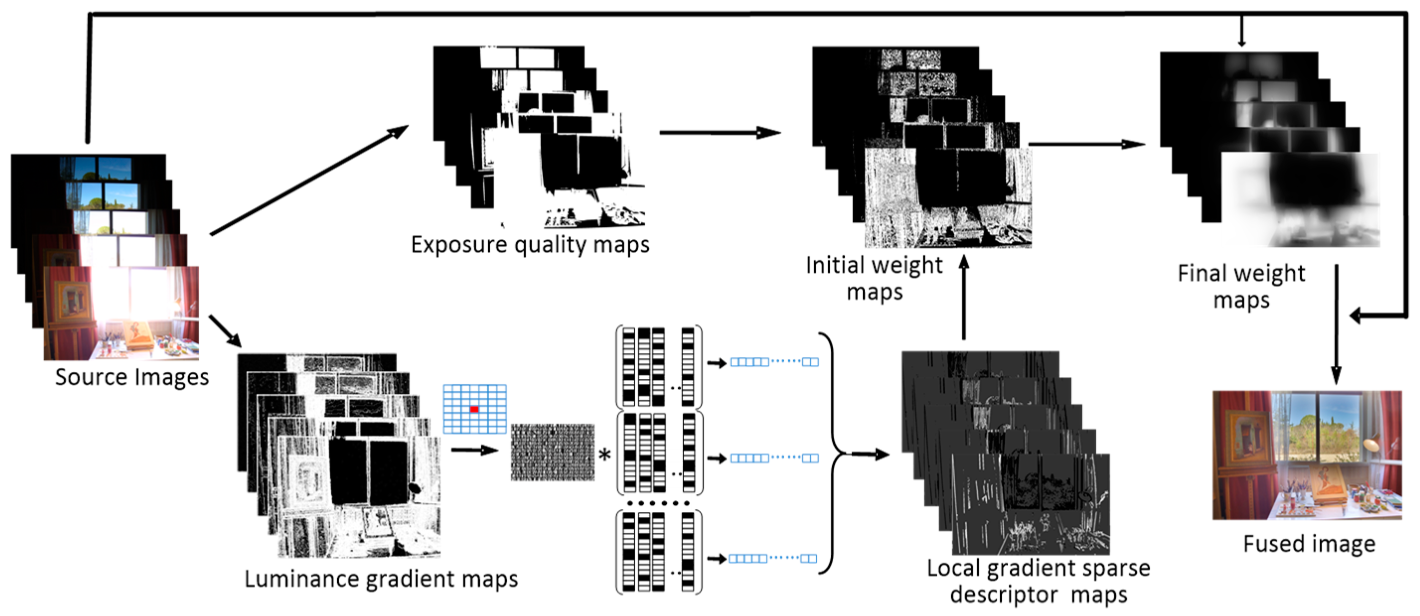
The schematic diagram of the proposed multi-exposure image fusion method, based on a sparse representation of gradient features, is shown in Figure 3. There are three steps in the proposed method: Image feature extraction, weight map calculation and weight term-based fusion. These image features are composed of a local gradient sparse descriptor and exposure quality.
3.1. Local Gradient Sparse Descriptor Extraction
The local gradient sparse descriptor is obtained by the sparse representation model. Since the digital signal can be represented with a linear combination of a “few” atoms from an over-complete dictionary [26,27], the inherent feature of the signal can be extracted through the sparse coefficient combination of the corresponding atoms. Mathematically, the digital signal y can be presented by the following model:
where denotes an over-complete dictionary, is an atom of the over-complete dictionary, and indicates the sparse coefficient vector, which has a value that can be obtained by solving the following optimization problem:
where denotes the l0-norm: The number of nonzero components.
Generally, there is noise in the original digital signal. Thus, the sparse representation model, including noise, can be expressed as
where ε > 0 is the error tolerance.
In the proposed method, the process of sparse representation is realized in two steps, namely dictionary learning and feature extraction.
3.1.1. Dictionary Learning in the Gradient Domain
During the process of sparse representation, it is meaningful to obtain a suitable over-complete dictionary [28]. Therefore, such a dictionary in the gradient domain should be obtained.
The dictionary learns from a large number of example image patches, using a certain training algorithm, such as K-means or K-SVD [29], and has better representative ability. Firstly, the luminance gradient map of the training image, I, is calculated:
where L is the operation for obtaining image luminance, and is the operation for obtaining the image gradient.
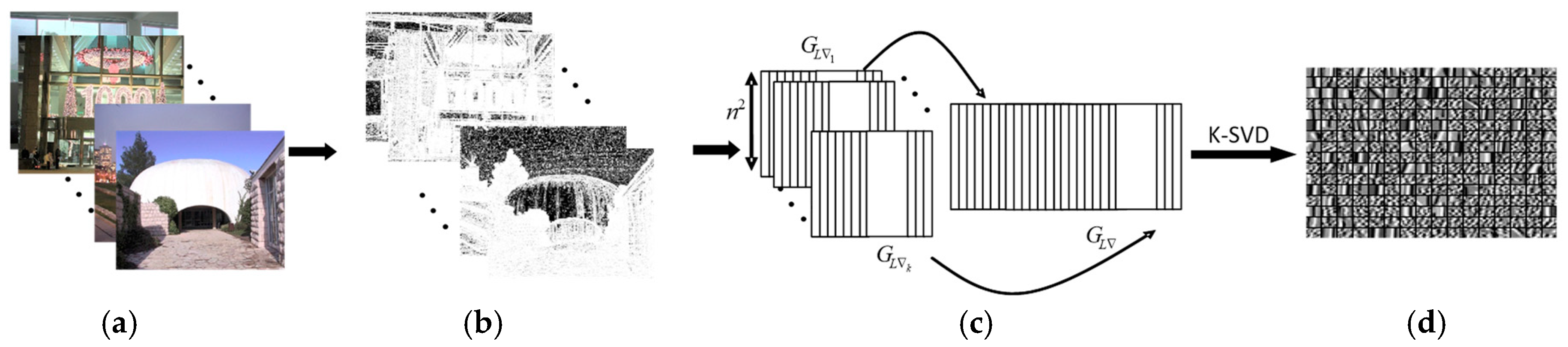
Then, the K-SVD algorithm is used to obtain the dictionary of gradient domain from the clear images of indoors and outdoors.
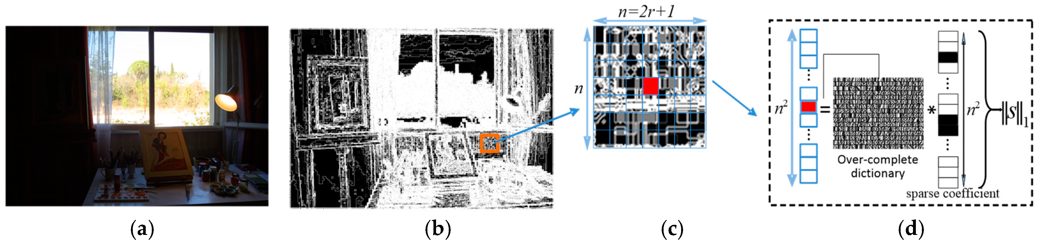
The dictionary learning framework in the gradient domain is shown in Figure 4. First, lots of luminance gradient maps are obtained from a large number of clear images, including indoors and outdoors. To construct the training set for dictionary learning from those luminance gradient maps, numerous image patches of size are randomly sampled in the same manner as Reference [30], but the patch size is odd, n = 2r + 1. Then, all of image patches are transformed into vectors via column by column extraction. Finally, the over-completed dictionary of the gradient domain can be obtained by the K-SVD algorithm.
3.1.2. Local Gradient Sparse Descriptor Extraction
During the process of local gradient sparse descriptor extraction, luminance gradient maps of the multi-exposure source images are obtained by Equation (4), as shown in Figure 5a,b. Then, the luminance gradient map, SL∇, is divided into overlapping image patches, as in Yang’s method [24]. However, the patch size is odd, n = 2r + 1, and as big as the patch size used in the dictionary learning. The next step is to shape each image patch into a vector through column-by-column extraction, as shown in Figure 5c,d. It is noteworthy that the small red piece in this figure represents the center of the image patch. Finally, each vector is now represented by a gradient domain from the over-complete dictionary obtained in the previous section, as shown in Figure 5d, wherein the black piece represents the nonzero sparse coefficient. Thus, the image patches can be expressed as:
where denotes the matrix that is lexicographically ordered from the luminance gradient maps, is the over-complete dictionary, is the sparse coefficient of each image patch, J is the number of image patches, and ε > 0 is the error tolerance. If , and , which is a sparse matrix, Equation (6) can be expressed as:
Then, the gradient sparse descriptor of the central pixel in the image patch, Ai(x, y), can be calculated as
where denotes the l1-norm, is the jth sparse matrix of the ith source image.
Generally, the larger the gradient value of the corresponding patch in multi-exposure source images, the better the exposure result of these regions, and the gradient sparse descriptor Ai(x, y) is also larger. However, in the HDR scenes, the invalid larger amplitude gradient may be found in a particular exposure source image, which does not represent a good exposure result. Fortunately, the gradients in the adjacent region of these invalid gradients are almost zero. So, the local gradient sparse descriptor Ai(x, y) of these regions is much smaller than the corresponding well-exposed image regions in other source images. Therefore, Ai(x,y) can effectively suppress the invalid large-amplitude gradients and remove halo artifacts from the fused image.
3.2. Exposure Quality Extraction
In the multi-exposure source images, there are more local details in the well-exposed regions. In the over-exposed or under-exposed regions, the luminance values are too extreme to present valid information. Therefore, the pixel luminance value is used to measure the local exposure quality. First, the luminance value of the images is normalized. Then, considering that there are more noises in the region under low illumination conditions, the exposure quality of pixels is calculated to obtain the exposure quality map:
where and are the thresholds, is the luminance map of the source image, and Bi(x, y) = 1 denotes that the related pixel is in the well-exposed region. Thus, the influence of over-exposed or under-exposed regions to the fused image can be effectively removed.
3.3. Initial Weight Map Estimation
After obtaining the local gradient sparse descriptor and exposure quality feature, the initial weight maps can be estimated by multiplying these two terms one-by-one:
Then, the weight maps, are normalized:
where denotes a small positive number (e.g., 10−25), which is used to avoid singularities in the weight value .
3.4. Final Weight Map Estimation and Fusion
Since the noises in the initial weight maps have greater influence on the fused image, the maps must be refined further. Considering the availability and real-time capability, the recursive filter [31], which can perform high-quality edge-preserving filtering of images in real time, is used to refine the initial weight maps:
where RF(•) presents the recursive filter operation, and Wi denotes the initial weight map, and Ii are the multi-exposure source images which can intensify the edge information during filtering.
After the final weight map has been normalized, the fused image, IF, can be obtained by:
and
4. Experiment and Analyses
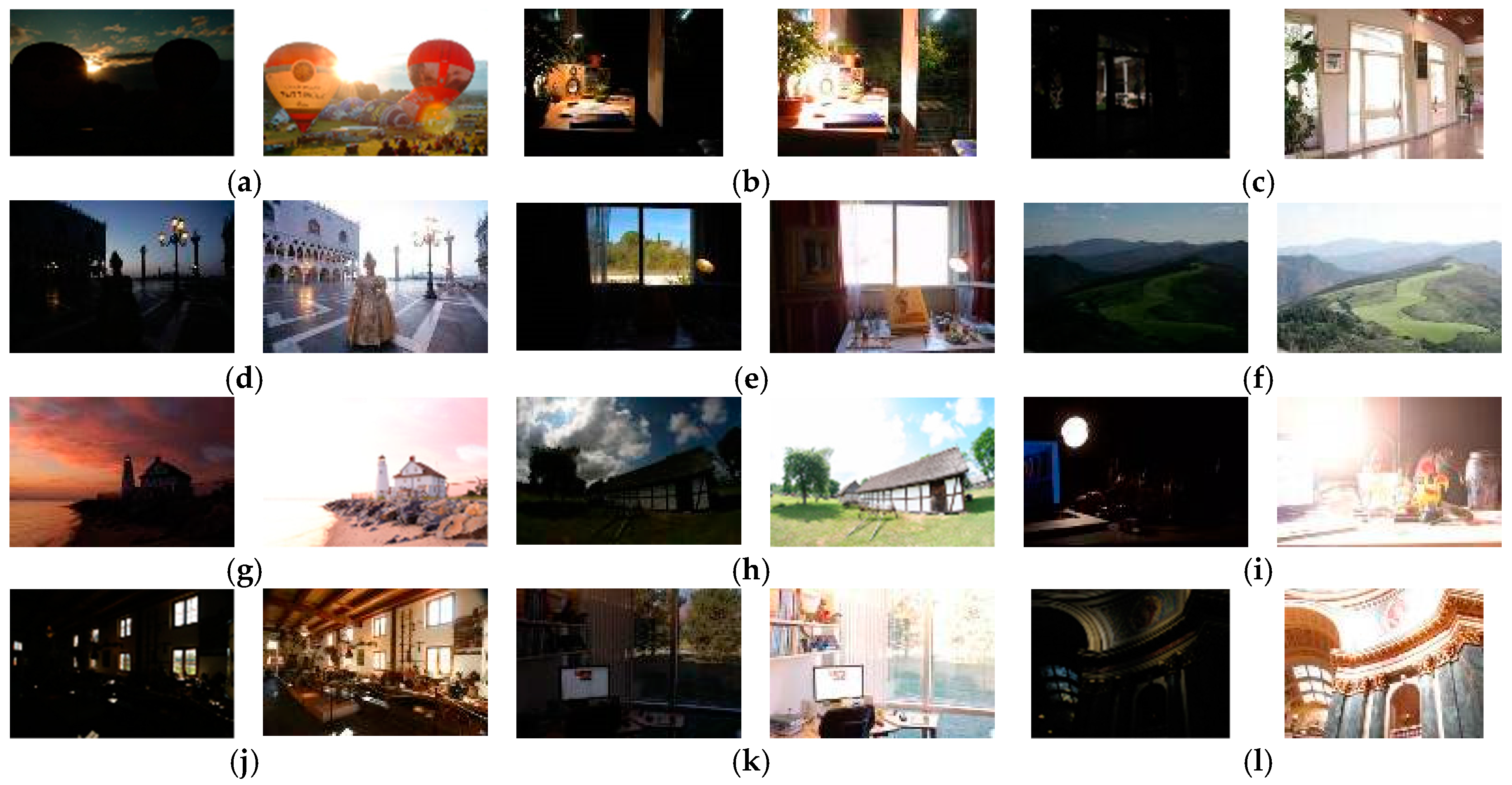
To compare the performance of the proposed multi-exposure fused method, 12 multi-exposure source image sequences, shot in different scenes with rich details and high brightness contrast, were used. Figure 6 shows two images of different exposures in each image sequence, as used in Ma et al.’s method [14], Merten’s method [15], and other databases. Additionally, more details of each multi-exposure source image sequence are described in Figure 6, including name, spatial resolution and number of source images. The experiment was run on a PC platform with an Intel® Core™ i5 processor with 4-GB memory.
In all of the following experiments, unless otherwise indicated, the parameters of the proposed method were as follows: the patch size, n, was fixed to 9 × 9; the global error was ε = 0.1; the threshold of exposure quality, , was set to 0.15; another threshold of exposure quality, α, was set to 0.05; and the parameter of the recursive filter was set to the optimal value, as in Liu’s method [12].
Five representative multi-exposure fused methods (i.e., Liu15 method [12], Ma18 method [14], Mertens10 method [15], Vonikakis11 method [16], Li13 method [18]) were employed to make comparisons via subjective and objective evaluation methods. The code of these fusion methods is available on the corresponding websites [32,33,34,35,36], and default parameters were used in the comparisons.
4.1. Subjective Evaluation
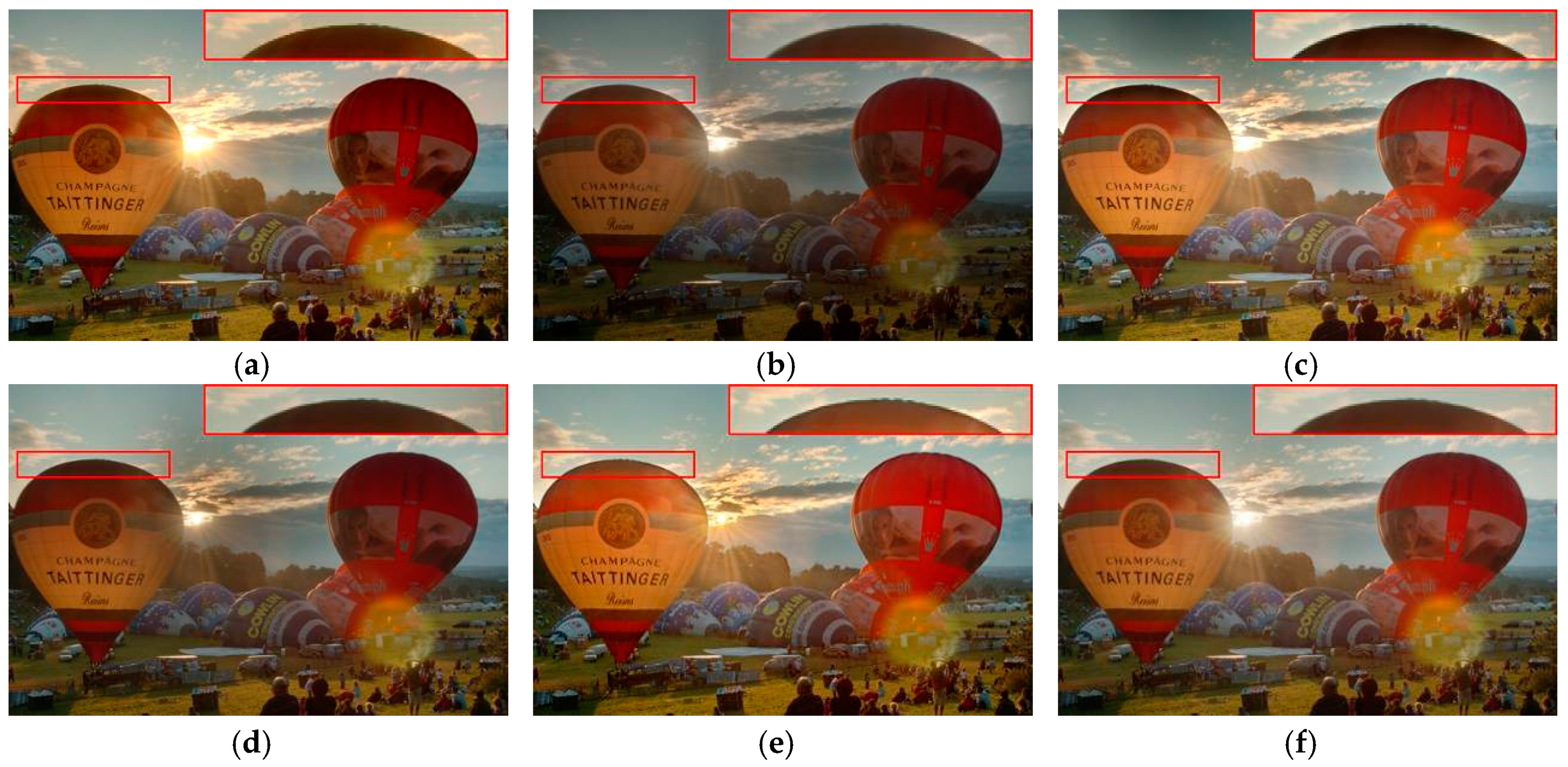
The subjective evaluation of the multi-exposure fusion methods is shown in Figure 7, Figure 8, Figure 9 and Figure 10. In Figure 7a, the results of Mertens10 showed nice global contrast and color information, but the details in the brighter regions are lost in the clouds around the sun. Halo artifacts are produced at the boundary between the balloon and the blue sky. Vonikakis11 can preserve the proper details in the brighter regions, but the details of the darker regions are lost at the lawn in the bottom of the balloon in Figure 7b, and halo artifacts are present. The best global contrast can be obtained with Li13 and Ma18, but the halo artifacts in those methods are more prominent. There are almost no halo artifacts in Liu15, but shadow can be observed around the sun. The fused image of the proposed method presented better visual perception and preserved the proper global contrast and color information (e.g., clouds around the sun and the lawn below the balloon), while simultaneously removing the halo artifacts.
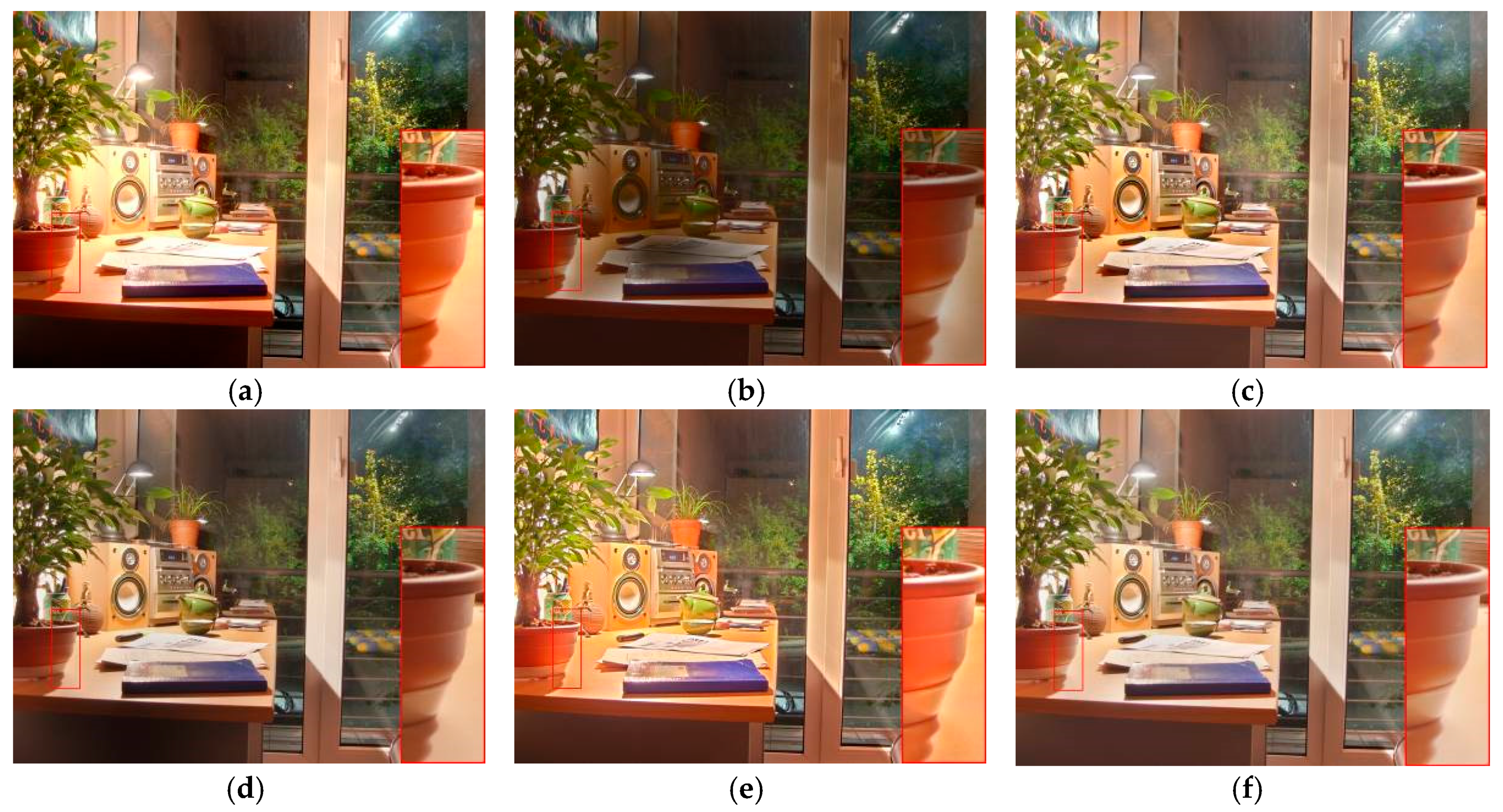
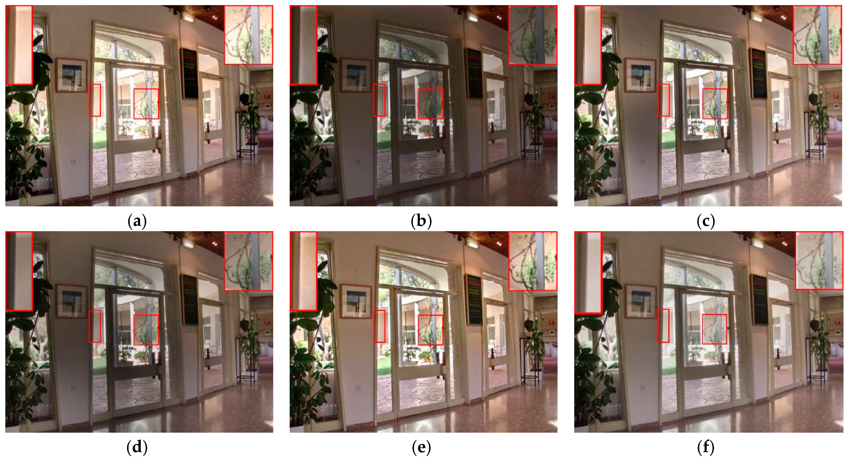
Figure 8 gives the results of an indoor scene. The results of Mertens10 showed nice global contrast, but the details, such as colors in the brighter regions, are lost (e.g., the details of the loudspeaker box on the left side). There are halo artifacts on the right side of the flowerpot. Additionally, the color is distorted, as shown in Figure 8e. Vonikakis11 also preserved the rich details in the brighter regions, but lost details in the darker regions (e.g., details of the outdoor scene in Figure 8b). Halo artifacts are also observed on the right side of the flowerpot. Halo artifacts in Li13, Liu15 and Ma18 are evident too. The proposed method had better global contrast and color information (e.g., vivid color in the loudspeaker box in Figure 8f), and overcame the halo artifacts present in the images produced via other methods.
The dynamic range of the scene in Figure 9 is not as wide as those in Figure 7 and Figure 8. However, it can also be seen that, in the Vonikakis11, Li13 and Ma18 method images, halo artifacts are observed near the doorframes in the middle of the fused images. There is also nice global contrast in the Mertens10 image, but the details, such as the background in the brighter regions, are lost (e.g., the details around the tree in the middle of the fused images). The results of Liu15 preserve the proper details in the brighter regions, but its global contrast is very limited. By contrast, the halo artifacts are removed with the proposed method, and proper global contrast and better visual perception are achieved.
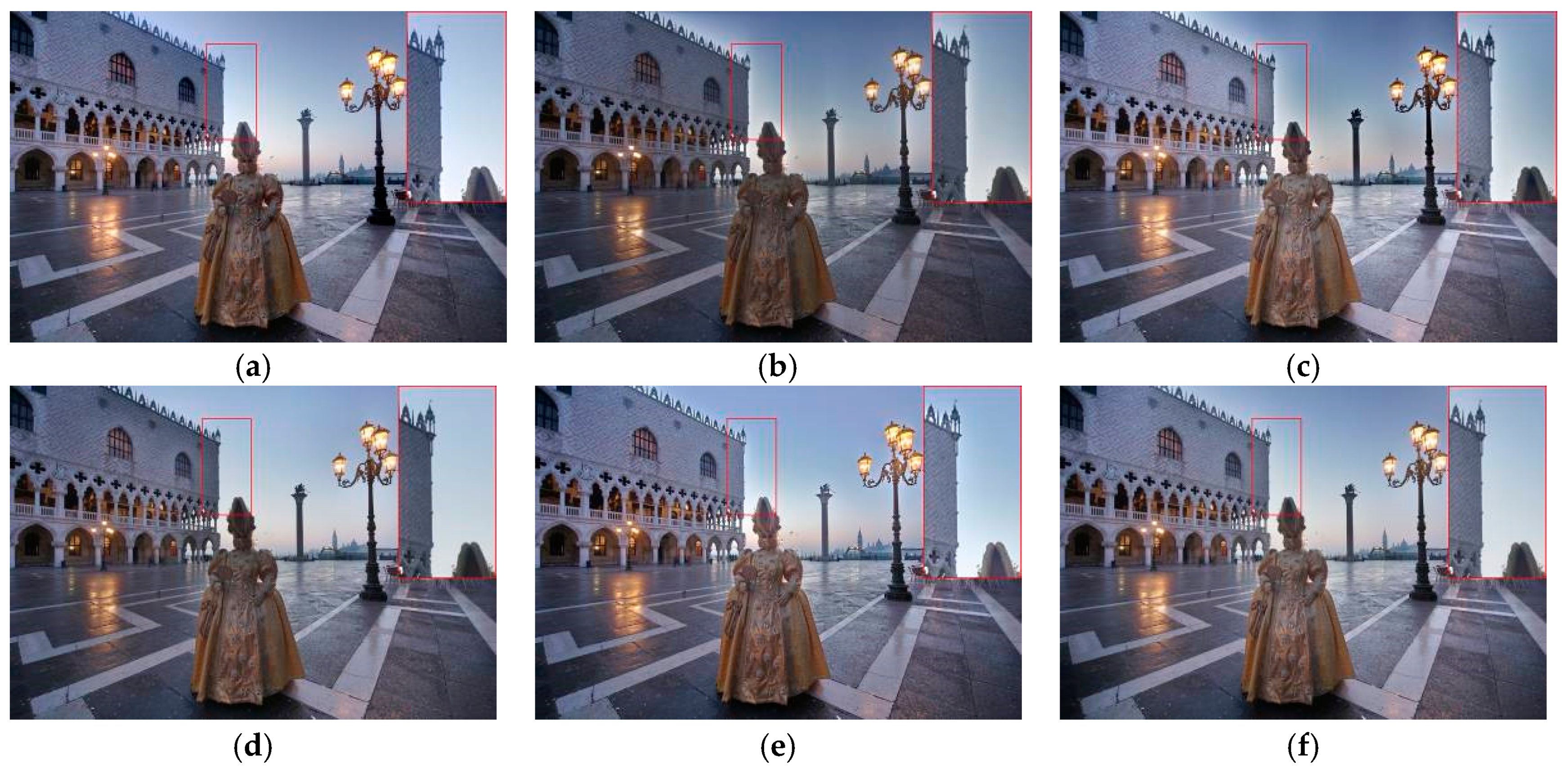
As can be clearly seen in Figure 10, there are halo artifacts on the right side of the palace and around the head of the performer, except with Liu15 and the proposed method. Although the halo artifacts are removed by Liu15, the color in the sky is distorted and became pale. However, the proposed method not only maintained better color information of the sky, but also removed the halo artifacts in the fused image.
4.2. Objective Evaluation
In this subsection, two objective metrics are applied to evaluate the performance of the different fused methods: QAB/F [37], MEF-SSIMc [38], and the distortion identification-based image verity and integrity evaluation (DIIVINE) [39], which is a no-reference image evaluation metric.
4.2.1. Evaluation Using QAB/F
The fusion metric, QAB/F, which is widely used in the fused image evaluation [12,24], can be extended to evaluate the image fused with three or more source images. This metric is mainly used to analyze the edge information of the fused images. The more edge information remaining, the larger the QAB/F value is. The extended version of QAB/F for multi-exposure fusion is defined as:
where denotes the fused image to be evaluated, , and are the edge intensity and orientation preservation values of the pixel at position , respectively, and is the gradient magnitude of , which is used as the weighting factor of .
4.2.2. The Structural Similarity Index (MEF-SSIMc)
The structural similarity index, MEF-SSIMc, represents the structure correlation between fused images and source images. The larger the MEF-SSIMc value, the closer the structure correlation. The formula of MEF-SSIMc is defined as:
where denotes the set of co-located image patches in the source image sequence, is the fused image. and denote the local variances of the source image and the fused image , and the local covariance between and , respectively. is a small positive stabilizing constant, is the spatial patch index and is the total number of patches.
The performance of the different methods on the 12 image sequences, using MEF-SSIMc, is listed in Table 2, where the top two values are shown in bold. According to the fusion metric, MEF-SSIMc, the performance of the proposed method was better than the other three compared methods and near to the Ma18 method. However, it was not as good as Mertens10, which uses contrast, saturation, and exposure quality to evaluate the source image exposure quality. However, this method may also lead to loss of details in the brighter regions, as shown in Figure 8a.
4.2.3. Evaluation Using DIIVINE
The multi-exposure fused image should not only retain more image information from the multi-exposure source images, but it should also match the human visual perception as closely as possible. Therefore, the non-reference image metric, DIIVINE, was introduced, based on perceived quality, into the fusion metric. DIIVINE evaluates the image quality through 88-dimensional image features, which are based on natural scene statistics. Meanwhile, DIIVINE is also capable of assessing the distorted image quality across multiple distortion categories. The larger the DIIVINE value, the more comfortable it is to human visual perception.
The performance of different methods on the 12 image sequences using DIIVINE is listed in Table 3. It can be seen that, in the fusion metric DIIVINE, the performance of the proposed method was superior to the other three comparative methods and near to the Liu15 method. However, it was not as good as Vonikakis11, which uses illumination estimation to evaluate the source image exposure quality. However, this method may also lead to loss of details in the blacker regions, as shown in Figure 9b.
4.3. Analysis of the Free Parameter
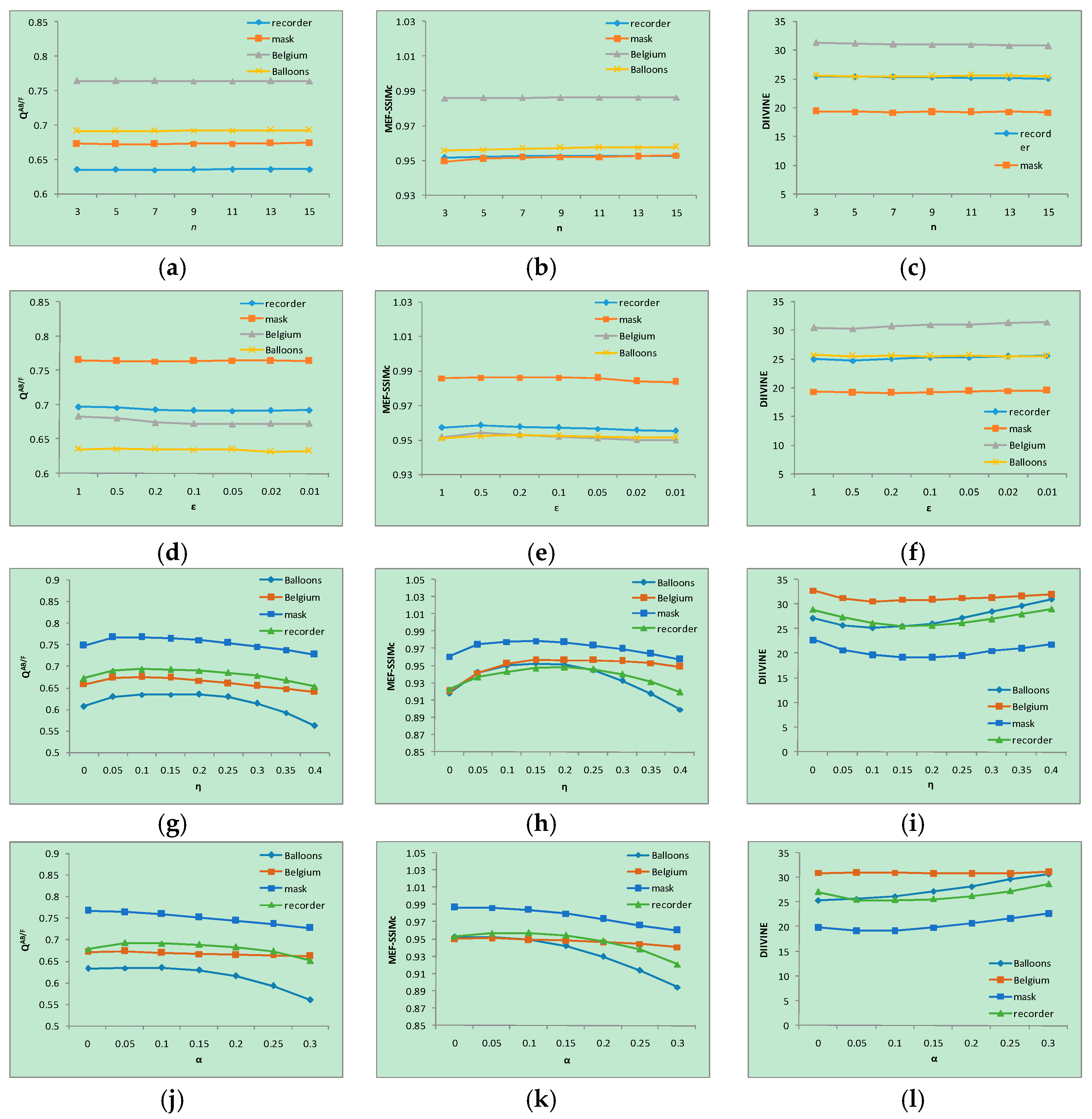
In this subsection, the influences of different parameters to objective fusion performances are presented and analyzed. The fusion performance was evaluated by the values of three fusion quality metrics, i.e., QAB/F, MEF-SSIMc and DIIVINE. When analyzing the influence of the patch size n, other parameters were set to ε = 0.1, α = 0.05 and = 0.15. Then, when analyzing the influence of ɛ, other parameters were set to n = 9, α = 0.05 and = 0.15. Next, α and were analyzed in the same way. As shown in Figure 12, with the increase of n, the value of QAB/F and MEF-SSIMc increased slowly, and the value of DIIVINE showed almost no fluctuation. Furthermore, with the decrease of ε, the value of QAB/F and MEF-SSIMc changed a little, while the value of DIIVINE has improved. When changing with and α, the value of QAB/F and MEF-SSIMc was worse if and α were too large or too small, and the value of DIIVINE showed only a slight concave change.
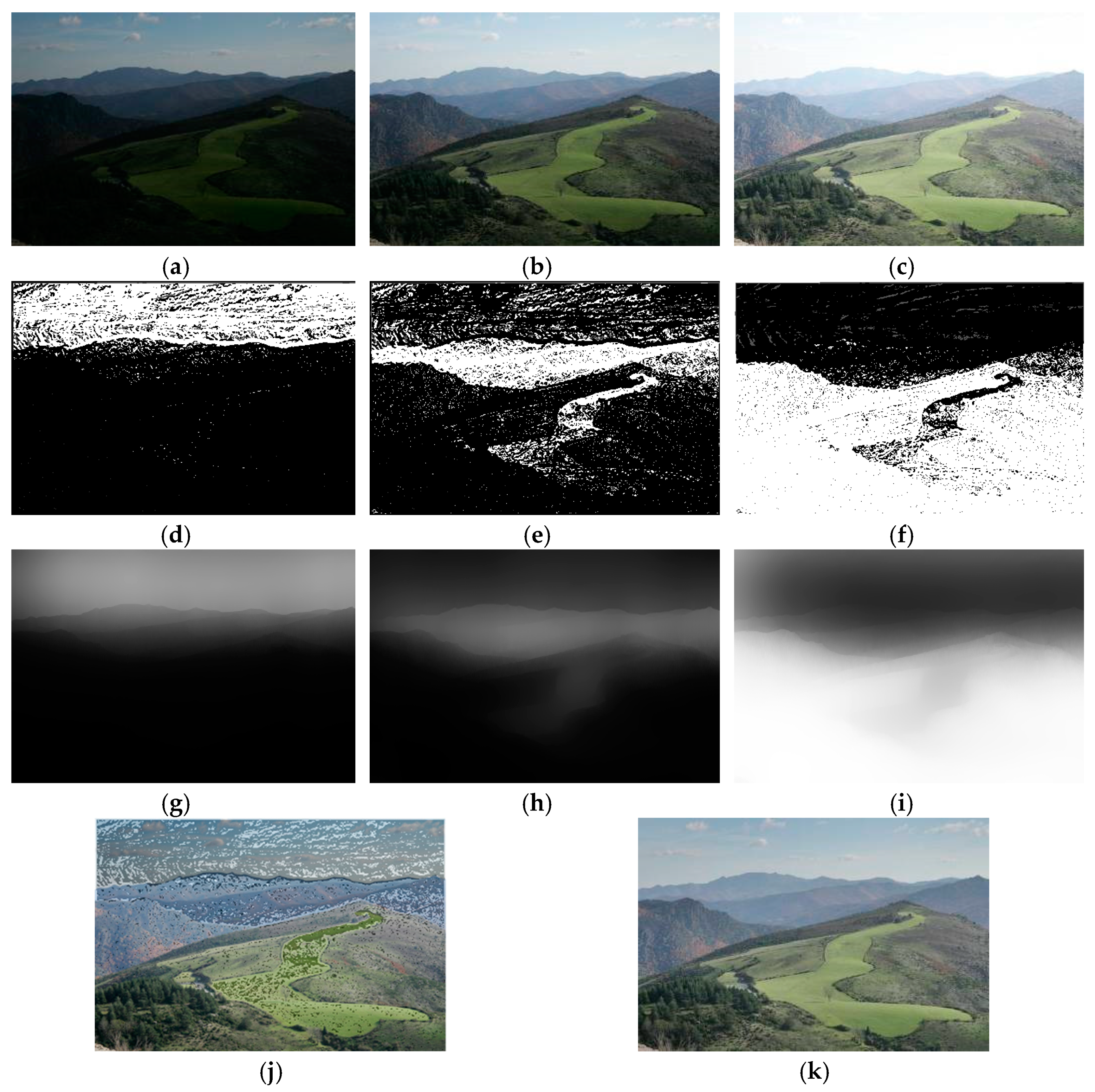
To better understand the proposed method, a set of comparative experiments were carried out to analyze the effect of the recursive filter in the fusion process. The experimental results show that the recursive filter can effectively remove the noise of the initial weight map and optimize the fusion result, as shown in Figure 13.
4.4. Computational Efficiency
In this subsection, the computational efficiency of the above six fusion methods, that is, the execution time of the corresponding methods in the computer, is compared, as listed in Table 4. Because of the high computational complexity of the sparse representation model, the proposed method spent most of its time on calculating the local gradient sparse descriptor of the source images. However, in the above six fusion methods, the proposed method had great efficiency improvement, compared to Ma18.
5. Conclusions
In this paper, we first analyzed the cause of halo artifacts in multi-exposure fused images. Then, we proposed a new multi-exposure fusion method based on sparse representation of gradient features. The sparse representation model was used to obtain the local gradient sparse descriptor, which can not only remove the halo artifacts, but can also extract image details effectively. The experiment was assessed through both a subjective and objective evaluation of 12 multi-exposure image sequences. Experimental results show that the proposed method was able to remove the halo artifacts and obtain a higher quality fused image, presenting a more vivid natural scene. In the future, we plan to assess whether the proposed method could be applied to multi-exposure image fusion in dynamic scenes.
Author Contributions
H.S. and G.J. designed the algorithm and wrote the source code. They together wrote the manuscript. M.Y. provided suggestions on the algorithm and revised the entire manuscript. Y.S., H.J., Z.P. and F.C. provided suggestions on the experiments.
Funding
The work was supported by the Natural Science Foundation of China (61671258, 61871247, 61771269, 61620106012), the Research Fund of Zhejiang Education Department (Y201635391), K.C. Wong Magna Fund of Ningbo University.
Conflicts of Interest
The authors declare no conflict of interest.
References
- Choi, I.; Baek, S.H.; Kim, M.H. Reconstructing Interlaced High-dynamic-range Video using Joint Learning. IEEE Trans. Image Process. 2017, 26, 5353–5366. [Google Scholar] [CrossRef] [PubMed]
- Nam, G.; Lee, H.; Oh, S.; Kim, M.H. Measuring Color Defects in Flat Panel Displays Using HDR Imaging and Appearance Modeling. IEEE Trans. Instrum. Meas. 2016, 65, 297–304. [Google Scholar] [CrossRef]
- Cauwerts, C.; Piderit, M.B. Application of High-Dynamic Range Imaging Techniques in Architecture: A Step toward High-Quality Daylit Interiors. J. Imaging 2018, 4, 19. [Google Scholar] [CrossRef]
- Artusi, A.; Richter, T.; Ebrahimi, T.; Mantiuk, R.K. High Dynamic Range Imaging Technology. IEEE Signal Process. Mag. 2017, 34, 165–172. [Google Scholar] [CrossRef]
- Richard, S. High dynamic range imaging. Opt. Eng. 2016, 52, 913–916. [Google Scholar]
- Kalantari, N.K.; Ramamoorthi, R. Deep High Dynamic Range Imaging of Dynamic Scenes. ACM Trans. Gr. 2017, 36, 1–12. [Google Scholar] [CrossRef]
- Huo, Y.; Zhang, X. Single image-based HDR image generation with camera response function estimation. Image Process. IET 2017, 11, 1317–1324. [Google Scholar] [CrossRef]
- Přibyl, B.; Chalmers, A.; Zemčík, P.; Hooberman, L.; Čadík, M. Evaluation of Feature Point Detection in High Dynamic Range Imagery. J. Vis. Commun. Image Represent. 2016, 38, 141–160. [Google Scholar] [CrossRef]
- Ji, W.; Park, R.; Chang, S. Local tone mapping using the K-means algorithm and automatic gamma setting. IEEE Trans. Consum. Electron. 2011, 57, 209–217. [Google Scholar]
- Khan, I.R.; Rahardja, S.; Khan, M.M.; Movania, M.M.; Abed, F. A tone-mapping technique based on histogram using a sensitivity model of the human visual system. IEEE Trans. Ind. Electron. 2018, 65, 3469–3479. [Google Scholar] [CrossRef]
- Eilertsen, G.; Mantiuk, R.K.; Unger, J. A Comparative Review of Tone Mapping Algorithms for High Dynamic Range Video. Comput. Gr. Forum 2017, 36, 565–592. [Google Scholar] [CrossRef]
- Liu, Y.; Wang, Z. Dense SIFT for Ghost-free Multi-exposure Fusion. J. Vis. Commun. Image Represent. 2015, 31, 208–224. [Google Scholar] [CrossRef]
- Ma, K.; Li, H.; Yong, H.; Wang, Z.; Meng, D.; Zhang, L. Robust Multi-Exposure Image Fusion: A Structural Patch Decomposition Approach. IEEE Trans. Image Process. 2017, 26, 2519–2532. [Google Scholar] [CrossRef] [PubMed]
- Ma, K.; Duanmu, Z.; Yeganeh, H.; Wang, Z. Multi-Exposure Image Fusion by Optimizing A Structural Similarity Index. IEEE Trans. Comput. Imaging 2018, 4, 60–72. [Google Scholar] [CrossRef]
- Mertens, T.; Kautz, J.; van Reeth, F. Exposure Fusion: A Simple and Practical Alternative to High Dynamic Range Photography. Comput. Gr. Forum 2010, 28, 161–171. [Google Scholar] [CrossRef]
- Vonikakis, V.; Bouzos, O.; Andreadis, I. Multi-exposure Image Fusion Based on Illumination Estimation. In Proceedings of the SIPA 2011, Crete, Greece, 22–24 June 2010; pp. 135–142. [Google Scholar]
- Zhang, W.; Cham, W.K. Gradient-directed Multi-exposure Composition. IEEE Trans. Image Process. 2012, 21, 2318–2323. [Google Scholar] [CrossRef] [PubMed]
- Li, S.; Kang, X.; Hu, J. Image Fusion with Guided Filtering. IEEE Trans. Image Process. 2013, 22, 28–64. [Google Scholar]
- Shen, J.; Zhao, Y.; Yan, S.; Li, X. Exposure Fusion using Boosting Laplacian Pyramid. IEEE Trans. Cybern. 2014, 44, 1579–1590. [Google Scholar] [CrossRef] [PubMed]
- Prabhakar, K.; Srikar, V.; Babu, R. DeepFuse: A Deep Unsupervised Approach for Exposure Fusion with Extreme Exposure Image. In Proceedings of the 2017 IEEE International Conference on Computer Vision (ICCV), Venice, Italy, 22–29 October 2017; pp. 4724–4732. [Google Scholar]
- Aharon, M.; Elad, M.; Bruckstein, A. K-SVD: An Algorithm for Designing Over-complete Dictionaries for Sparse Representation. IEEE Trans. Signal Process. 2006, 54, 4311–4322. [Google Scholar] [CrossRef]
- He, Z.; Yi, S.; Cheung, Y.M.; You, X.; Tang, Y.Y. Robust object tracking via key patch sparse representation. IEEE Trans. Cybern. 2017, 47, 354–364. [Google Scholar] [CrossRef] [PubMed]
- Qin, H.; Han, J.; Yan, X.; Zeng, Q.; Zhou, H.; Li, J.; Chen, Z. Infrared small moving target detection using sparse representation-based image decomposition. Infrared Phys. Technol. 2016, 76, 148–156. [Google Scholar] [CrossRef]
- Yang, B.; Li, S. Multi-focus Image Fusion and Restoration with Sparse Representation. IEEE Trans. Instrum. Meas. 2010, 59, 884–892. [Google Scholar] [CrossRef]
- Liu, Y.; Liu, S.; Wang, Z. A General Framework for Image Fusion Based on Multi-scale Transform and Sparse Representation. Inf. Fusion 2015, 24, 147–164. [Google Scholar] [CrossRef]
- Bruckstein, A.M.; Donoho, D.L.; Elad, M. From Sparse Solutions of Systems of Equations to Sparse Modeling of Signals and Images. SIAM Rev. 2009, 51, 34–81. [Google Scholar] [CrossRef] [Green Version]
- Elad, M.; Figueiredo, M.A.T.; Ma, Y. On the Role of Sparse and Redundant Representations in Image Processing. Proc. IEEE 2010, 98, 972–982. [Google Scholar] [CrossRef] [Green Version]
- Cheng, J.; Liu, H.; Liu, T.; Wang, F.; Li, H. Remote Sensing Image Fusion via Wavelet Transform and Sparse Representation. ISPRS J. Photogramm. Remote Sens. 2015, 104, 158–173. [Google Scholar] [CrossRef]
- Cai, J.; Cheng, Q.; Peng, M.; Song, Y. Fusion of infrared and visible images based on nonsubsampled contourlet transform and sparse K-SVD dictionary learning. Infrared Phys. Technol. 2017, 82, 85–95. [Google Scholar] [CrossRef]
- Liu, Y.; Wang, Z. Simultaneous image fusion and denoising with adaptive sparse representation. Image Process. Iet 2014, 9, 347–357. [Google Scholar] [CrossRef]
- Gastal, E.S.L.; Oliveira, M.M. Domain transform for edge-aware image and video processing. ACM Trans. Gr. 2011, 30, 69–80. [Google Scholar] [CrossRef]
- T. Mertens Software. Available online: http://jankautz.com/ (accessed on 7 January 2018).
- S. Li Software. Available online: http://xudongkang.weebly.com/ (accessed on 7 January 2018).
- V. Vonikakis Software. Available online: http://vonikakis.com/ (accessed on 12 March 2018).
- Y. Liu Software. Available online: http://www.escience.cn/people/liuyu1/Codes.html (accessed on 7 January 2018).
- K. Ma Software. Available online: https://ece.uwaterloo.ca/~k29ma/ (accessed on 5 April 2018).
- Xydeas, C.S.; Petrovic, V.S. Objective Image Fusion Performance Measure. Electron. Lett. 2000, 36, 308–309. [Google Scholar] [CrossRef]
- Ma, K.; Zeng, K.; Wang, Z. Perceptual Quality Assessment for Multi-Exposure Image Fusion. IEEE Trans. Image Process. 2015, 20, 3345–3356. [Google Scholar] [CrossRef] [PubMed]
- Moorthy, A.K.; Bovik, A.C. Blind Image Quality Assessment: From Natural Scene Statistics to Perceptual Quality. IEEE Trans. Image Process. 2011, 20, 3350–3364. [Google Scholar] [CrossRef] [PubMed]
Figure 1.
An example of multi-exposure image fusion. (a) The fused image by Li et al. [18], and (b) the fused image by the proposed method.
Figure 1.
An example of multi-exposure image fusion. (a) The fused image by Li et al. [18], and (b) the fused image by the proposed method.

Figure 2.
Local luminance gradient comparison of multi-exposure source images: (a–e) multi-exposure source images; (f–j) luminance gradient maps; and (k–o) luminance gradient amplitude of the red lines in (f–j).
Figure 2.
Local luminance gradient comparison of multi-exposure source images: (a–e) multi-exposure source images; (f–j) luminance gradient maps; and (k–o) luminance gradient amplitude of the red lines in (f–j).

Figure 3.
Schematic diagram of the proposed multi-exposure.

Figure 4.
Dictionary learning in the gradient domain: (a) Clear images of indoors and outdoors; (b) Luminance gradient map; (c) Lexicographical vector; (d) Over-complete dictionary.
Figure 4.
Dictionary learning in the gradient domain: (a) Clear images of indoors and outdoors; (b) Luminance gradient map; (c) Lexicographical vector; (d) Over-complete dictionary.

Figure 5.
Local gradient sparse descriptor acquisition: (a) Input image; (b) Input luminance gradient map; (c) Luminance gradient patch; (d) Local gradient sparse descriptor‖S‖1.
Figure 5.
Local gradient sparse descriptor acquisition: (a) Input image; (b) Input luminance gradient map; (c) Luminance gradient patch; (d) Local gradient sparse descriptor‖S‖1.

Figure 6.
Multi-exposure source image sequences used in the experiments: (a) “balloons”, 512 × 339 × 9 (the sequence contains a total of nine images, and the spatial resolution of each is 512 × 339); (b) “recorder”, 1024 × 768 × 13; (c) “Belgium House”, 512 × 384 × 9; (d) “mask”, 1200 × 800 × 3; (e) “StudioEV”, 1200 × 800 × 5; (f) “landscape”, 512 × 341 × 3; (g) “lighthouse”, 512 × 340 × 3; (h) “Kluki”, 512 × 341 × 3; (i) “desk”, 640 × 427 × 7; (j) “farm house”, 512 × 341 × 3; (k) “office”, 512 × 340 × 6; and (l) “Madison Capitol”, 512 × 384 × 30.

Figure 7.
Performance comparison of different methods on the “balloons” image sequence. (a) Mertens10 [15]; (b) Vonikakis11 [16]; (c) Li13 [18]; (d) Liu15 [12]; (e) Ma18 [14]; and (f) the proposed method.

Figure 8.
Performance comparison of different methods on the “recorder” image sequence. (a) Mertens10 [15]; (b) Vonikakis11 [16]; (c) Li13 [18]; (d) Liu15 [12]; (e) Ma18 [14]; and (f) the proposed method.

Figure 9.
Performance comparison of different methods on the “Belgium House” image sequence. (a) Mertens10 [15]; (b) Vonikakis11 [16]; (c) Li13 [18]; (d) Liu15 [12]; (e) Ma18 [14]; and (f) the proposed method.

Figure 10.
Performance comparison of different methods on the “Mask” image sequence. (a) Mertens10 [15]; (b) Vonikakis11 [16]; (c) Li13 [18]; (d) Liu15 [12]; (e) Ma18 [14]; and (f) the proposed method.

Figure 11.
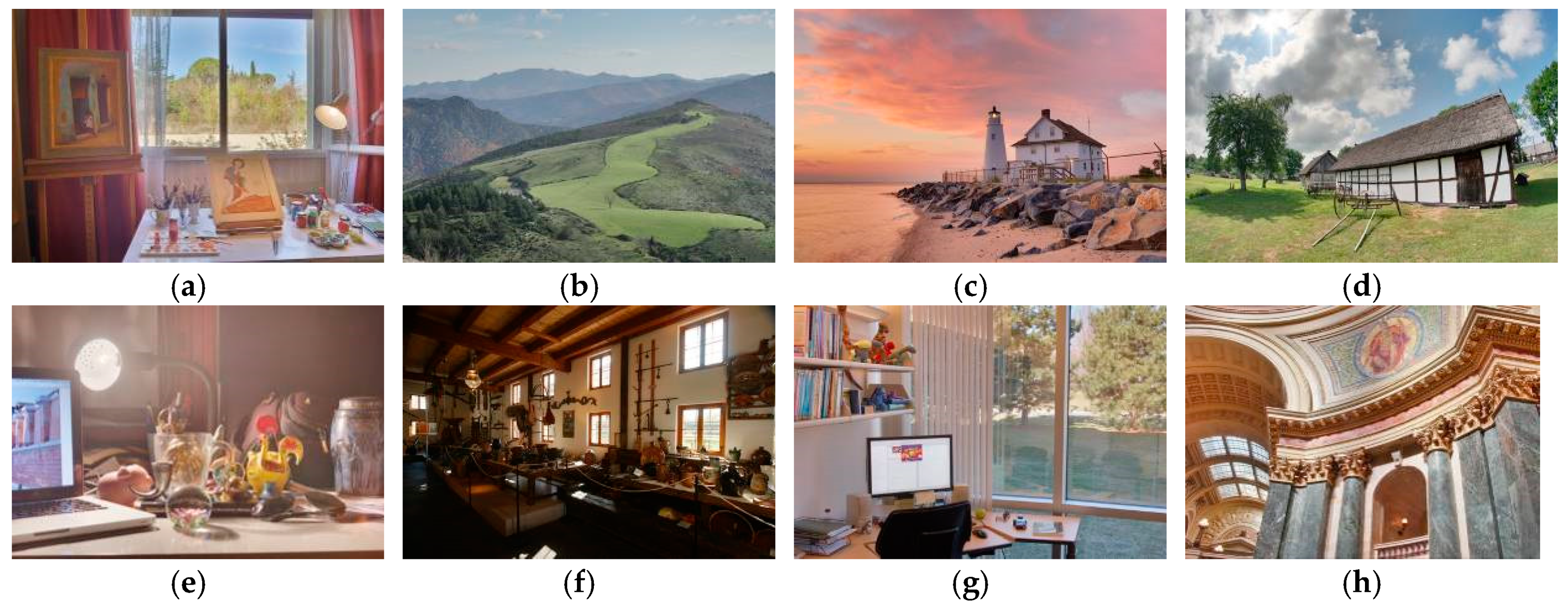
Other fused images of the proposed method. (a) Studio EV; (b) Landscape; (c) Lighthouse; (d) Kluki; (e)desk; (f) Farmhouse; (g) Office; and (h) Madison Capitol.
Figure 11.
Other fused images of the proposed method. (a) Studio EV; (b) Landscape; (c) Lighthouse; (d) Kluki; (e)desk; (f) Farmhouse; (g) Office; and (h) Madison Capitol.

Figure 12.
Performance of the proposed method with different parameters, i.e., (a) QAB/F ~ n, (b) MEF-SSIMc ~ n, (c) DIIVINE ~ n, (d) QAB/F ~ ε, (e) MEF-SSIMc ~ ε, (f) DIIVINE ~ ε, (g) QAB/F ~ η, (h) MEF-SSIMc ~ η, (i) DIIVINE ~ η, (j) QAB/F ~ α, (k) MEF-SSIMc ~ α, (l) DIIVINE ~ α.
Figure 12.
Performance of the proposed method with different parameters, i.e., (a) QAB/F ~ n, (b) MEF-SSIMc ~ n, (c) DIIVINE ~ n, (d) QAB/F ~ ε, (e) MEF-SSIMc ~ ε, (f) DIIVINE ~ ε, (g) QAB/F ~ η, (h) MEF-SSIMc ~ η, (i) DIIVINE ~ η, (j) QAB/F ~ α, (k) MEF-SSIMc ~ α, (l) DIIVINE ~ α.

Figure 13.
Performance comparison of fusion results between without recursive filter and with recursive filter. (a–c) multi-exposure source images; (d–f) weight map without recursive filter; (g–i) weight map with recursive filter; (j) fused image without recursive filter; and (k) fused image with recursive filter.


Table 1.
Performance of different methods on the 12 image sequences, using [37]. Top two values are shown in bold.
Table 1.
Performance of different methods on the 12 image sequences, using [37]. Top two values are shown in bold.
| Image | Method | |||||
|---|---|---|---|---|---|---|
| Mertens10 [15] | Vonikakis11 [16] | Li13 [18] | Liu15 [12] | Ma18 [14] | The Proposed Method | |
| balloons | 0.6210 | 0.5493 | 0.5940 | 0.6333 | 0.6137 | 0.6340 |
| recorder | 0.6784 | 0.4483 | 0.6720 | 0.6970 | 0.6479 | 0.6923 |
| Belgium | 0.6500 | 0.5563 | 0.6650 | 0.6608 | 0.6447 | 0.6724 |
| mask | 0.7484 | 0.7201 | 0.7451 | 0.7646 | 0.7396 | 0.7636 |
| Studio EV | 0.6748 | 0.6297 | 0.6812 | 0.6870 | 0.6712 | 0.6802 |
| landscape | 0.7530 | 0.6805 | 0.7307 | 0.7874 | 0.7496 | 0.7749 |
| lighthouse | 0.7037 | 0.6860 | 0.6823 | 0.7326 | 0.7012 | 0.7245 |
| Kluki | 0.7604 | 0.7558 | 0.7539 | 0.7815 | 0.7435 | 0.7883 |
| desk | 0.6188 | 0.5324 | 0.6179 | 0.6201 | 0.6088 | 0.6314 |
| farmhouse | 0.7334 | 0.7409 | 0.7486 | 0.7855 | 0.7411 | 0.7758 |
| office | 0.7500 | 0.7449 | 0.7331 | 0.7665 | 0.7268 | 0.7727 |
| Madison | 0.7289 | 0.4884 | 0.7154 | 0.7316 | 0.6934 | 0.7389 |
| Average | 0.7017 | 0.6277 | 0.6949 | 0.7207 | 0.6901 | 0.7208 |
Table 2.
Performance of different methods on the 12 image sequences, using the structural similarity index (MEF-SSIMc) [38]. Top two values are shown in bold.
Table 2.
Performance of different methods on the 12 image sequences, using the structural similarity index (MEF-SSIMc) [38]. Top two values are shown in bold.
| Image | Method | |||||
|---|---|---|---|---|---|---|
| Mertens10 [15] | Vonikakis11 [16] | Li13 [18] | Liu15 [12] | Ma18 [14] | The Proposed Method | |
| balloons | 0.9694 | 0.8887 | 0.9476 | 0.9239 | 0.9619 | 0.9527 |
| recorder | 0.9738 | 0.8128 | 0.9393 | 0.9441 | 0.9469 | 0.9567 |
| Belgium House | 0.9709 | 0.8340 | 0.9639 | 0.9053 | 0.9660 | 0.9513 |
| mask | 0.9854 | 0.9609 | 0.9670 | 0.9663 | 0.9862 | 0.9863 |
| StudioEV | 0.9752 | 0.9256 | 0.9544 | 0.9397 | 0.9528 | 0.9530 |
| landscape | 0.9762 | 0.9520 | 0.9421 | 0.9799 | 0.9775 | 0.9777 |
| lighthouse | 0.9802 | 0.9547 | 0.9501 | 0.9681 | 0.9547 | 0.9690 |
| Kluki | 0.9801 | 0.9560 | 0.9482 | 0.9550 | 0.9636 | 0.9638 |
| desk | 0.9497 | 0.8421 | 0.9219 | 0.8970 | 0.9245 | 0.9227 |
| farmhouse | 0.9810 | 0.9398 | 0.9647 | 0.9616 | 0.9804 | 0.9633 |
| office | 0.9845 | 0.9609 | 0.9674 | 0.9663 | 0.9854 | 0.9786 |
| Madison capitol | 0.9773 | 0.9433 | 0.9479 | 0.9175 | 0.9619 | 0.9472 |
| Average | 0.9780 | 0.9142 | 0.9512 | 0.9437 | 0.9635 | 0.9602 |
Table 3.
Performance of different methods on the 12 image sequences, using the distortion identification-based image verity and integrity evaluation (DIIVINE) [39]. Top two values are shown in bold.
Table 3.
Performance of different methods on the 12 image sequences, using the distortion identification-based image verity and integrity evaluation (DIIVINE) [39]. Top two values are shown in bold.
| Image | Methods | |||||
|---|---|---|---|---|---|---|
| Mertens10 [15] | Vonikakis11 [16] | Li13 [17] | Liu15 [12] | Ma18 [14] | The Proposed Method | |
| balloons | 21.690 | 29.398 | 20.773 | 25.045 | 20.126 | 25.593 |
| recorder | 17.581 | 36.836 | 16.897 | 25.917 | 13.666 | 25.491 |
| Belgium | 24.099 | 33.065 | 23.308 | 30.987 | 21.113 | 30.946 |
| mask | 17.136 | 23.309 | 15.985 | 19.982 | 15.702 | 19.219 |
| Studio EV | 33.391 | 37.526 | 31.926 | 36.211 | 29.878 | 37.892 |
| landscape | 13.843 | 9.859 | 13.523 | 20.893 | 13.837 | 16.623 |
| lighthouse | 17.752 | 24.927 | 17.068 | 21.068 | 15.045 | 20.761 |
| Kluki | 6.3632 | 6.4153 | 6.217 | 12.443 | 5.480 | 9.122 |
| desk | 34.468 | 39.936 | 33.863 | 39.397 | 31.580 | 39.907 |
| farmhouse | 17.334 | 21.604 | 16.954 | 21.104 | 15.976 | 22.142 |
| office | 25.077 | 31.479 | 24.850 | 30.809 | 23.507 | 29.931 |
| Madison | 10.490 | 22.561 | 12.076 | 14.709 | 14.761 | 15.102 |
| Average | 19.935 | 26.410 | 19.453 | 24.880 | 18.389 | 24.395 |
Table 4.
Computational efficiency of different fused methods on the 12 image sequences (s).
| Images | Methods | |||||
|---|---|---|---|---|---|---|
| Mertens10 [15] | Vonikakis11 [16] | Li13 [17] | Liu15 [12] | Ma18 [14] | The Proposed Method | |
| balloons | 2.729 | 4.870 | 3.595 | 15.720 | 542.91 | 70.95 |
| recorder | 8.970 | 23.746 | 20.795 | 109.393 | 3648.04 | 682.64 |
| Belgium | 2.875 | 5.123 | 3.971 | 16.913 | 618.89 | 184.52 |
| mask | 4.444 | 9.517 | 7.854 | 21.172 | 2891.22 | 227.85 |
| Studio EV | 4.207 | 12.599 | 10.088 | 29.607 | 3076.38 | 214.51 |
| landscape | 0.880 | 1.528 | 1.090 | 3.349 | 466.07 | 26.63 |
| lighthouse | 0.870 | 1.558 | 1.114 | 3.140 | 587.42 | 38.36 |
| Kluki | 0.868 | 1.507 | 1.159 | 3.371 | 467.69 | 61.65 |
| desk | 2.379 | 5.134 | 4.290 | 15.456 | 1178.81 | 116.54 |
| farmhouse | 0.885 | 1.464 | 1.406 | 3.392 | 413.87 | 78.03 |
| office | 1.623 | 2.622 | 2.292 | 8.320 | 405.25 | 112.92 |
| Madison | 7.947 | 12.931 | 13.656 | 125.060 | 918.81 | 789.35 |
© 2018 by the authors. Licensee MDPI, Basel, Switzerland. This article is an open access article distributed under the terms and conditions of the Creative Commons Attribution (CC BY) license (http://creativecommons.org/licenses/by/4.0/).
Share and Cite
MDPI and ACS Style
Shao, H.; Jiang, G.; Yu, M.; Song, Y.; Jiang, H.; Peng, Z.; Chen, F. Halo-Free Multi-Exposure Image Fusion Based on Sparse Representation of Gradient Features. Appl. Sci. 2018, 8, 1543. https://doi.org/10.3390/app8091543
AMA Style
Shao H, Jiang G, Yu M, Song Y, Jiang H, Peng Z, Chen F. Halo-Free Multi-Exposure Image Fusion Based on Sparse Representation of Gradient Features. Applied Sciences. 2018; 8(9):1543. https://doi.org/10.3390/app8091543
Chicago/Turabian StyleShao, Hua, Gangyi Jiang, Mei Yu, Yang Song, Hao Jiang, Zongju Peng, and Feng Chen. 2018. "Halo-Free Multi-Exposure Image Fusion Based on Sparse Representation of Gradient Features" Applied Sciences 8, no. 9: 1543. https://doi.org/10.3390/app8091543
Note that from the first issue of 2016, this journal uses article numbers instead of page numbers. See further details here.