Article

Construction of Measurement Matrix Based on Cyclic Direct Product and QR Decomposition for Sensing and Reconstruction of Underwater Echo

1
Department of Automation, Hangzhou Dianzi University, Xiasha Higher Education Zone, Hangzhou 310018, China
2
Department of Physics, University of Bath, Claverton Down, Bath BA2 7AY, UK
*
Author to whom correspondence should be addressed.
Appl. Sci. 2018, 8(12), 2510; https://doi.org/10.3390/app8122510
Submission received: 28 October 2018 / Revised: 27 November 2018 / Accepted: 3 December 2018 / Published: 6 December 2018
(This article belongs to the Section Acoustics and Vibrations)

Abstract

:
Compressive sensing is a very attractive technique to detect weak signals in a noisy background, and to overcome limitations from traditional Nyquist sampling. A very important part of this approach is the measurement matrix and how it relates to hardware implementation. However, reconstruction accuracy, resistance to noise and construction time are still open challenges. To address these problems, we propose a measurement matrix based on a cyclic direct product and QR decomposition (the product of an orthogonal matrix Q and an upper triangular matrix R). Using the definition and properties of a direct product, a set of high-dimensional orthogonal column vectors is first established by a finite number of cyclic direct product operations on low-dimension orthogonal “seed” vectors, followed by QR decomposition to yield the orthogonal matrix, whose corresponding rows are selected to form the measurement matrix. We demonstrate this approach with simulations and field measurements of a scaled submarine in a freshwater lake, at frequencies of 40 kHz–80 kHz. The results clearly show the advantage of this method in terms of reconstruction accuracy, signal-to-noise ratio (SNR) enhancement, and construction time, by comparison with Gaussian matrix, Bernoulli matrix, partial Hadamard matrix and Toeplitz matrix. In particular, for weak signals with an SNR less than 0 dB, this method still achieves an SNR increase using less data.

1. Introduction

Compressive sensing (CS) is a rapidly emerging technique [1,2,3]. Its main attraction is that it can overcome the shortcomings of the traditional Nyquist sampling theorem [4] in signal processing, in terms of the large amount of data to be sampled and large data storage space required, because signal sampling and compression are performed simultaneously. CS is widely applied in medical image processing [5], image compression [6,7], pattern recognition [8,9], and radar detection [10]; it can also be combined with the Bayesian algorithm [11,12], e.g., to reconstruct underwater echoes. CS involves three key components: (1) the sparse representation of the signal [13]; (2) the construction of a measurement matrix [14]; and (3) signal reconstruction [15,16]. The second step, construction of a measurement matrix, is particularly important as it directly affects the performance of signal reconstruction and is an indispensable part of sampling systems based on CS, thereby determining their possible applications in actual engineering situations.
Measurement matrices commonly used in CS are random or deterministic. The former are currently more popular in the literature, and include the Gaussian matrix [17], the sparse projection matrix [18], and the Bernoulli matrix [19,20]. These matrices are nearly orthogonal; they are thus more likely to satisfy the restricted isometry property (RIP), will require less measurements, and will provide strong signal reconstruction performance. However, they need a large storage space, and suffer from high computational volume and time complexity, which makes their hardware implementation difficult. Conversely, deterministic measurement matrices show lower computational complexity and easier hardware implementation. For example, the partial Hadamard matrix [21], the Toeplitz matrix [22,23], and polynomial matrices [24], whose elements possess higher certainty than random measurement matrices, are frequently used in this field. Signal reconstruction, however, is less satisfactory, and more measurements are needed to accurately reconstruct the signal.
Studies show that the reconstruction performance of the measurement matrix can be improved by reducing the cross-correlation coefficient between the measurement matrix and the sparse matrix [25] and improving the nonlinear correlation of the measurement matrix. The performance in terms of signal reconstruction and the number of measurements needed depend closely on the cross-correlation coefficient. A minor number of measurements are required for signal reconstruction if the cross-correlation coefficient is small, and the signal is adaptive over a larger sparsity range. Nonlinear correlation is a very important property of the measurement matrix, by which the performance is better and signal recovery is more accurate if the nonlinear correlation is higher. However, how would it work in practice?
After more explanations of compressive sensing and construction of the measurement matrix (Section 2), this study shows how it can construct by combining the cyclic direct product and QR decomposition (Section 3) possessing less correlation with the sparse matrix and between its own column vectors (let us remember that the QR decomposition of a matrix A formulates it as the product A = QR of an orthogonal matrix Q and an upper triangular matrix R, and is often used to solve the linear least squares problem). It is thus more likely to satisfy the RIP [26,27] required for the measurement matrix to ensure high-accuracy reconstruction with low computational complexity. This is tested with simulations of underwater echoes (Section 4) and corresponding experimental measurements of echoes from a scaled submarine target in a freshwater lake (Section 5).

2. Compressive Sensing and Measurement Matrix

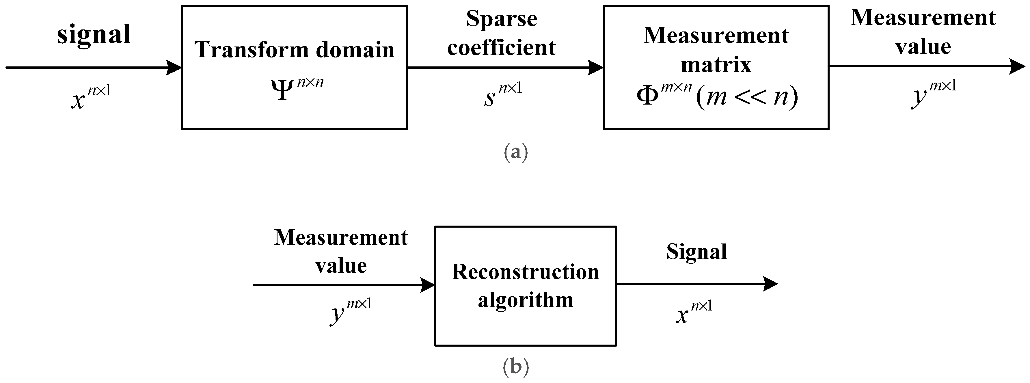
2.1. Compressive Sensing (CS)

The signal x R N is called the K -sparse signal if it only has K ( K N ) nonzero coefficients. The measured signal y = Φ x is obtained by compression and projection. Φ R M × N ( M N ) is called the measurement matrix, where M is the number of measurements. Using the measured signal y and the measurement matrix Φ , the original signal x ^ can be recreated by the reconstruction algorithm through the process depicted in Figure 1 [28].
Since signal x is sparse and its recovery involves inversion, signal reconstruction can be regarded as the search of the solutions with the least number of non-zero coefficients from all possible solutions, i.e., the solutions that minimize l 0 or l 1 norm below:
min s l 0 s . t . y = Φ x , min s l 1 s . t . y = Φ x
In summary, CS takes place in the following steps: a suitable measurement matrix is constructed when sparse representation or compressibility of the original signal under a certain sparse basis is possible; the original signal of higher dimension is projected onto low-dimensional space using this matrix; the original signal is restored accurately or with high probability from the observed data with a reconstruction algorithm.

2.2. Measurement Matrix

The key in signal observation by CS is the construction of the measurement matrix. Using the same sparse matrix and reconstruction algorithm but different measurement matrices, better signal reconstruction is achieved by higher-performance measurement matrices. Candès et al. [2,3] formulated the famous restricted isometry principle, which is a required condition on the measurement matrix for it to recover the original signal without distortion.
In the RIP, for signal x with length N and sparsity K, let Φ be the measurement matrix of dimension M × N, and I be the set of subscripts corresponding to the K columns selected from Φ and having a number of elements less than or equal to the sparsity K. If a constant exists that makes the following inequality valid:
( 1 δ K ) x 2 2 Φ I x 2 2 ( 1 + δ K ) x 2 2 ,
then the matrix Φ is said to satisfy the K-restricted isometry property, which is written in short as R I P ( K , δ K ) .
Despite its perfect form and rich connotation, RIP cannot be used to guide the construction of a particular measurement matrix, as it is only a necessary but not a sufficient condition. According to the study by Donoho [29], the measurement matrix must satisfy the following three conditions: (1) the column vectors of a measurement matrix must possess certain linear independence; (2) the column vectors are random and independent; and (3) the solution that satisfies the sparsity is the vector that makes the norm minimum. These three characteristics are decisive in the construction of the measurement matrix, while other considerations include: (1) the amount of data should be as small as possible; (2) hardware implementation and possibility of algorithm optimization; and (3) broad applicability.
Two basis vectors that are orthogonal are mutually independent, i.e., they have no correlation with each other. Therefore, the measurement matrix could be orthogonalized to achieve pairwise independence between the vectors, and made practical for CS. It is known from matrix properties that the singular values of a matrix are closely related to its linear correlation property. A larger least singular value indicates greater independence among the column vectors of the matrix. When the least singular value approaches zero, the matrix tends to singularity. It is thus possible to construct a measurement matrix based on this idea to achieve the desired effect.

3. Construction of Measurement Matrix by Cyclic Direct Product and QR Decomposition

3.1. Definition of Direct Product

Let A = ( α i j ) m × n and B = ( β i j ) p × q ; then, the mp × nq matrix will be given by
[ α 11 B α 12 B α 1 n B α 21 B α 22 B α 2 n B α m 1 B α m 2 B α m n B ] .
This matrix is called the Kronecker product or direct product [30] of A and B, and is denoted as AB.
An important property of the direct product is as follows: let χ1, χ2, …, χn be N numbers of linearly independent m-dimensional column vectors, and y1, y2, …, yq be q numbers of linearly independent p-dimensional column vectors; it then follows that the nq numbers of mp-dimensional column vectors χiyj (i = 1, 2, …, n; j = 1, 2, …, n) are linearly independent, and vice versa.
From the properties of the direct product, it is possible to generate higher-dimension matrices from lower-dimension ones, and make the resulting column vectors linearly independent. The key to this method is to select a set of well-behaving lower-dimension orthogonal column vectors as the “seed sequence” to ensure mutual orthogonality in the set of higher-dimension column vectors constructed by the cyclic direct product, and the maximum non-correlation possible among the row vectors. From the definition of the direct product, the number of cyclic direct products performed is related to the dimension of the “seed” vectors n and the dimension of the higher-dimension column vectors N, such that the number of cyclic computations k = logn N, as in the case of k = logn N = log21024 = 10. Compared with conventional higher-dimension matrices and their construction, the cyclic direct product is easier to perform and greatly saves matrix construction time.

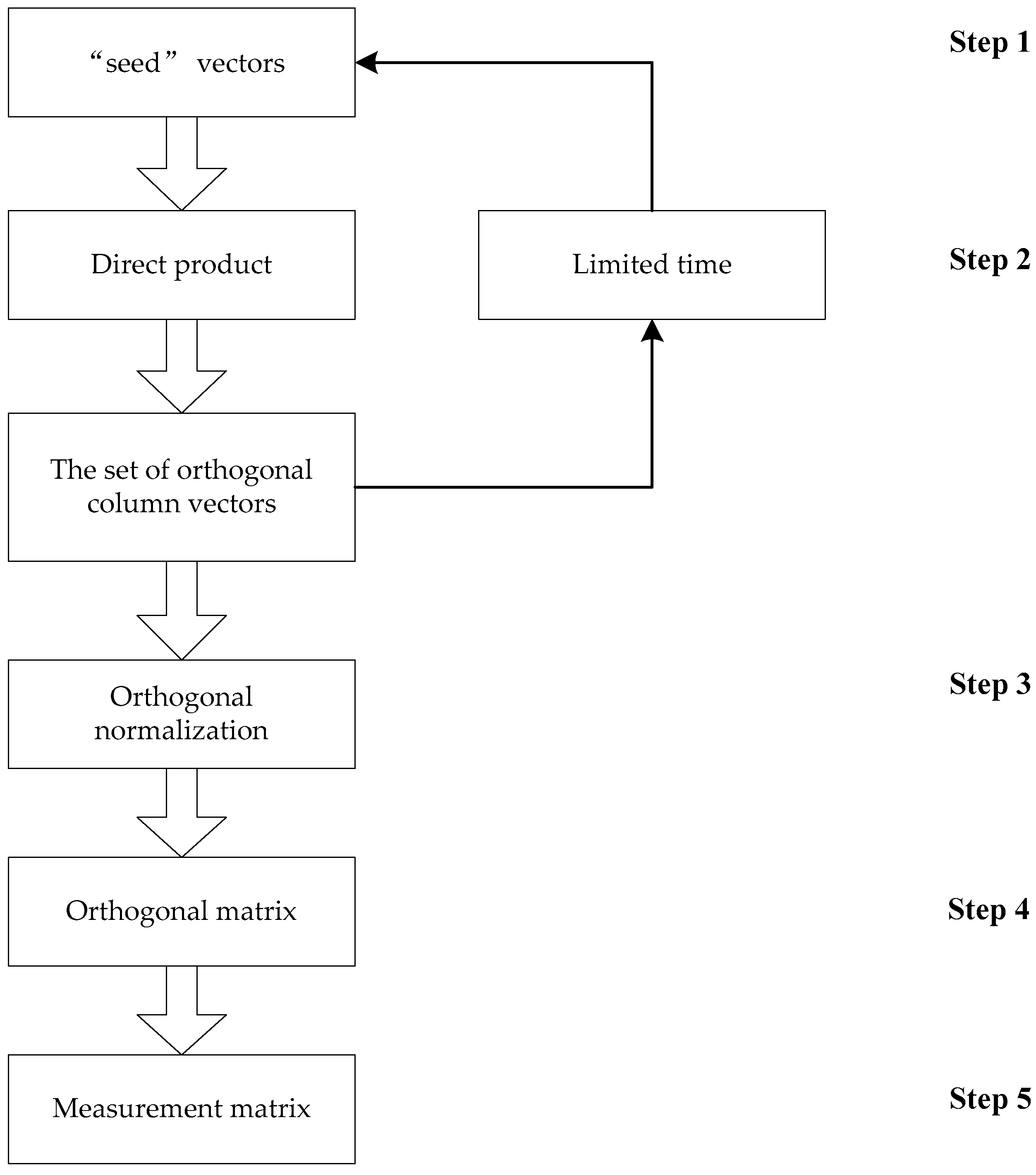
3.2. Construction of Measurement Matrix Based On Cyclic Direct Product and QR Decomposition

As stated in Section 3.1, a high-dimension matrix could be constructed by taking the direct product, and applied to the computation of the measurement matrix for CS, i.e., the formation of a high-dimension orthogonal column vector set by finite times of cyclic direct product operation on lower-dimension orthogonal “seed” vectors, yielding a matrix with orthogonal column vectors. M rows are selected from this matrix to afford the corresponding deterministic measurement matrix. However, the high-dimension column vector set could only ensure mutual independence among the columns of the matrix thus formed, while the elements of the column vectors were still highly similar. When an appropriate number of measurements M is used for the construction of the measurement matrix, the column vectors may lose their pairwise orthogonality. As described in the introduction, the measurement matrix should possess column vectors with the highest possible linear independence. In an orthogonal matrix, the number of rows is far less than the number of columns. As determined by its structure, the maximum rank of a measurement matrix thus equals the number of rows, which means that linear correlation necessarily exists for this class of matrix.
The solution to the above problems lies in reducing the correlation between the column vectors. QR decomposition [31] of a matrix increases the singular value of the matrix without altering the properties of the measurement matrix, thus bringing the column vectors closer to being linearly independent. Specifically, QR decomposition is applied to the matrix composed of the set of higher-dimension orthogonal column vectors to obtain an orthogonal matrix, whose corresponding rows are selected to construct the measurement matrix. The detailed steps are shown in Figure 2.
Step 1. Suitable low-dimension orthogonal “seed” vectors are selected. The number of these vectors is equal to its dimension N. In the ideal case, the matrix U formed by these “seed” vectors is an orthogonal matrix with UUT = E, where E is the identity matrix. One example of U is [ 1 1 1 1 ] , which meets the required pairwise orthogonality among the row vectors and column vectors.
Step 2. The number of cyclic direct product computations, k ≈ logn N, is calculated using the dimension n of the “seed” vector and the dimension N of the higher-dimension column vectors, giving the initial value R1 = U, Ri = Ri−1U, while i = 2, 3, …, k.
Step 3. The matrix Rk obtained after k cycles is a matrix of the order N with mutually orthogonal row vectors and column vectors. By theorems related to the QR decomposition of matrix analysis, an orthogonal matrix can be obtained by decomposition.
Step 4. M (M is the number of measurements) rows are selected from Uk to give the measurement matrix, i.e., the matrix by the QR decomposition of the cyclic direct product.
Φ = U k ( c , : ) , in which c is the set of subscripts for the rows selected, and Φ is the measurement matrix generated by the QR decomposition of the cyclic direct product.
Step 5. The measurement matrix is normalized in conformance to the RIP.
After the above procedures, the non-correlation among the column vectors of the measurement matrix formed by the cyclic product and QR decomposition is significantly improved. QR decomposition increases the least singular value of the matrix and further enhances its nonlinearity and independence, fulfilling the criteria for the measurement matrix. From the matrix theory, the measurement matrix constructed by QR decomposition satisfies the RIP. This measurement matrix given by the cyclic direct product and QR decomposition is deterministic, which greatly facilitates its engineering and implementation.

4. Testing the Performance of Measurement Matrix Using Simulated Underwater Echo

4.1. Parameters Used in Performance Testing
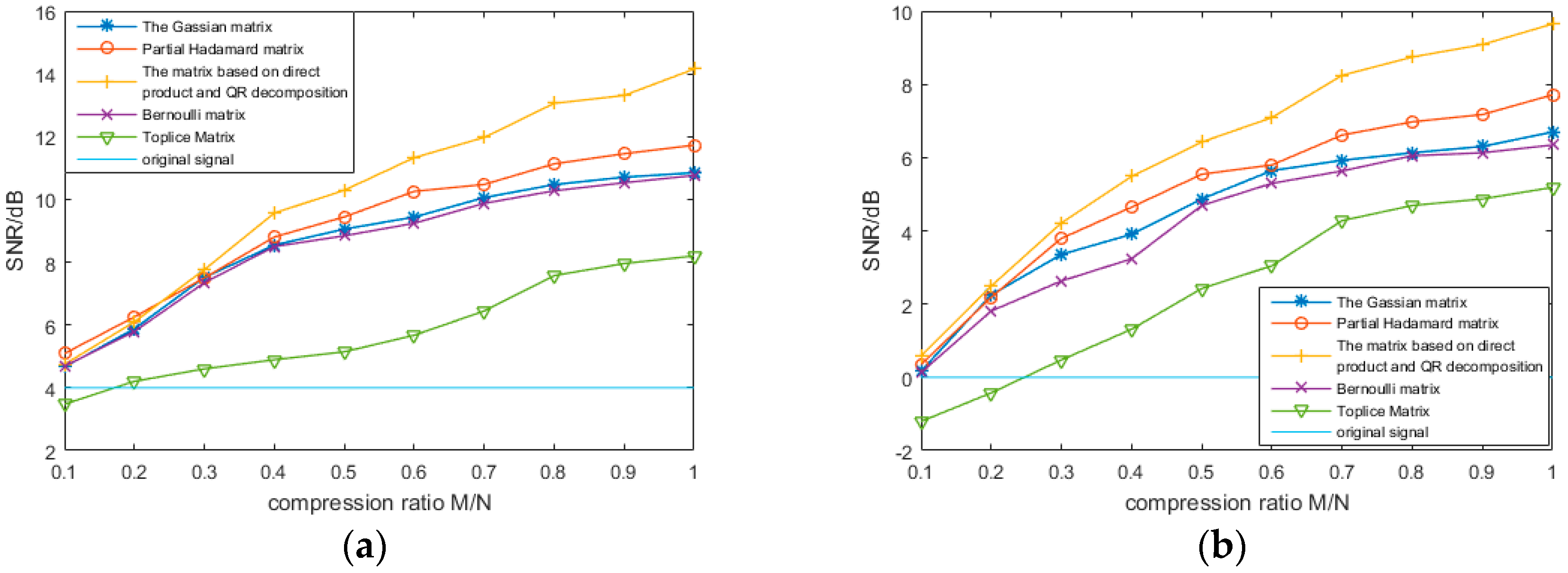
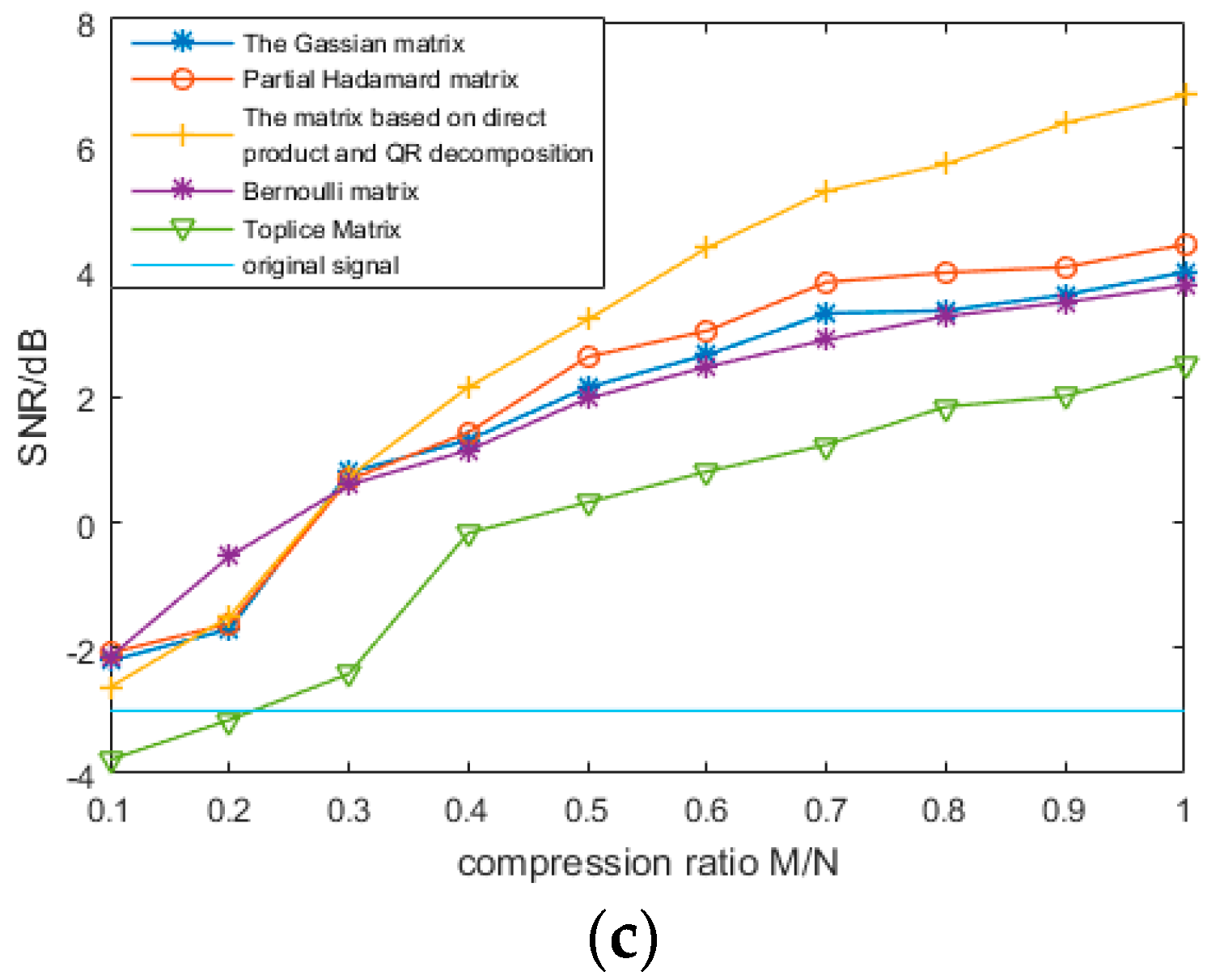
Let X be the original signal and X ^ be the recovered signal. The following evaluation indices are defined:
(a)
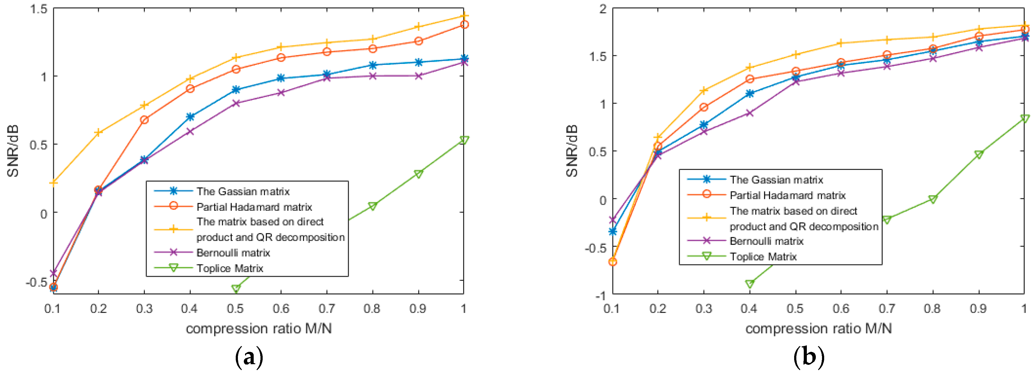
Signal-to-noise ratio:
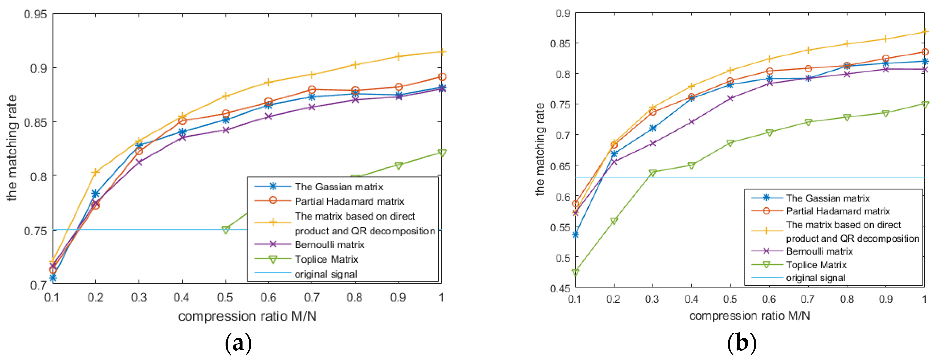
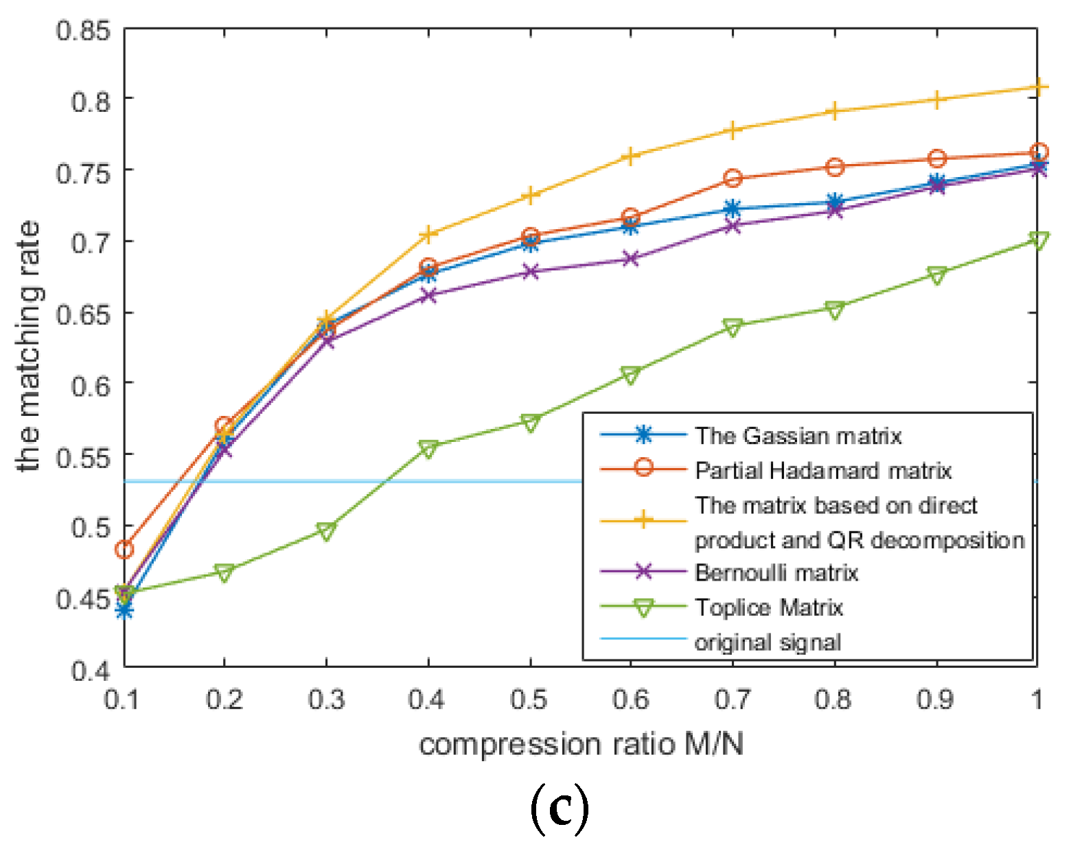
S N R = 10 lg ( X ^ 2 2 X X ^ 2 2 ) ,
(b)
Matching rate:
M a t c h i n g r a t e = 1 X ^ X 2 X ^ + X 2 ,
In which X ^ and X’ are the absolute values of X ^ and X.

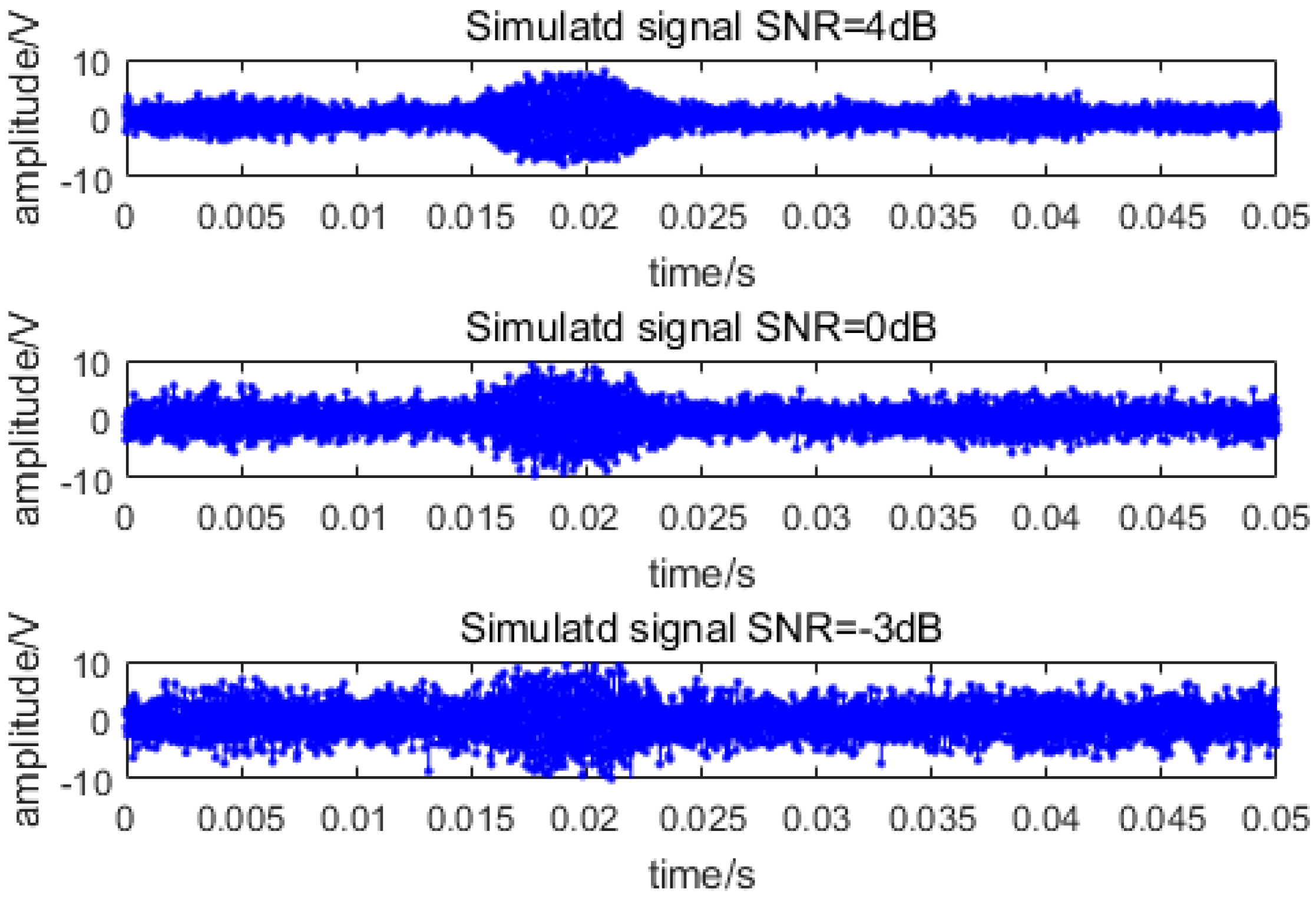
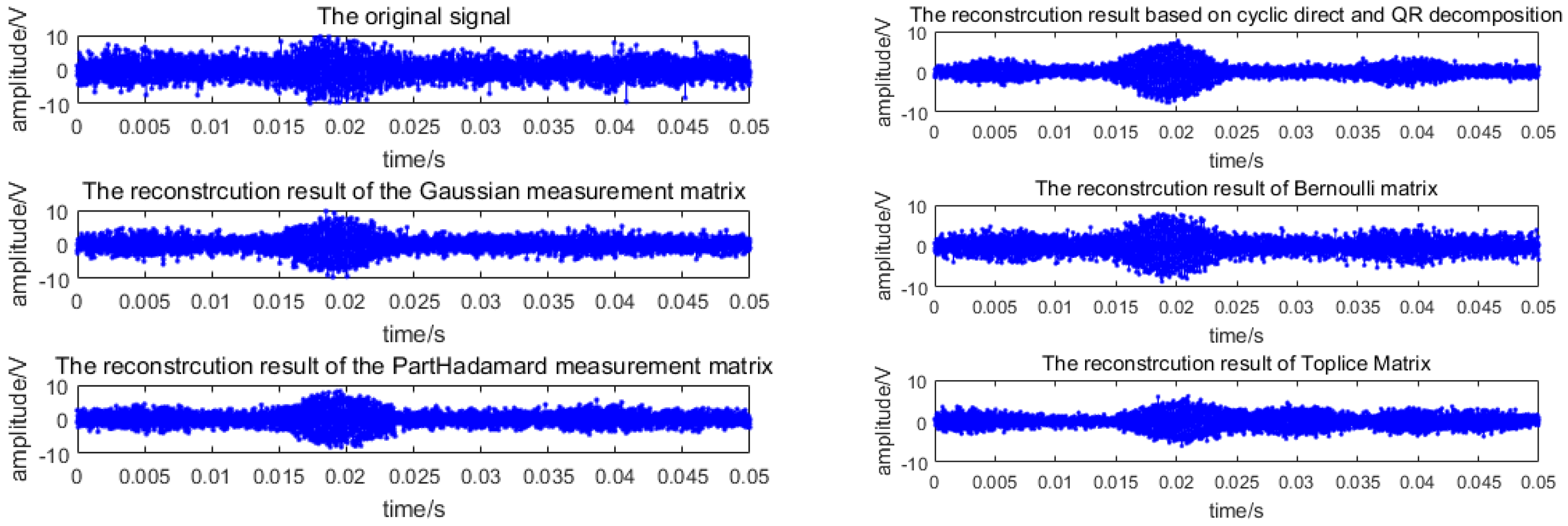
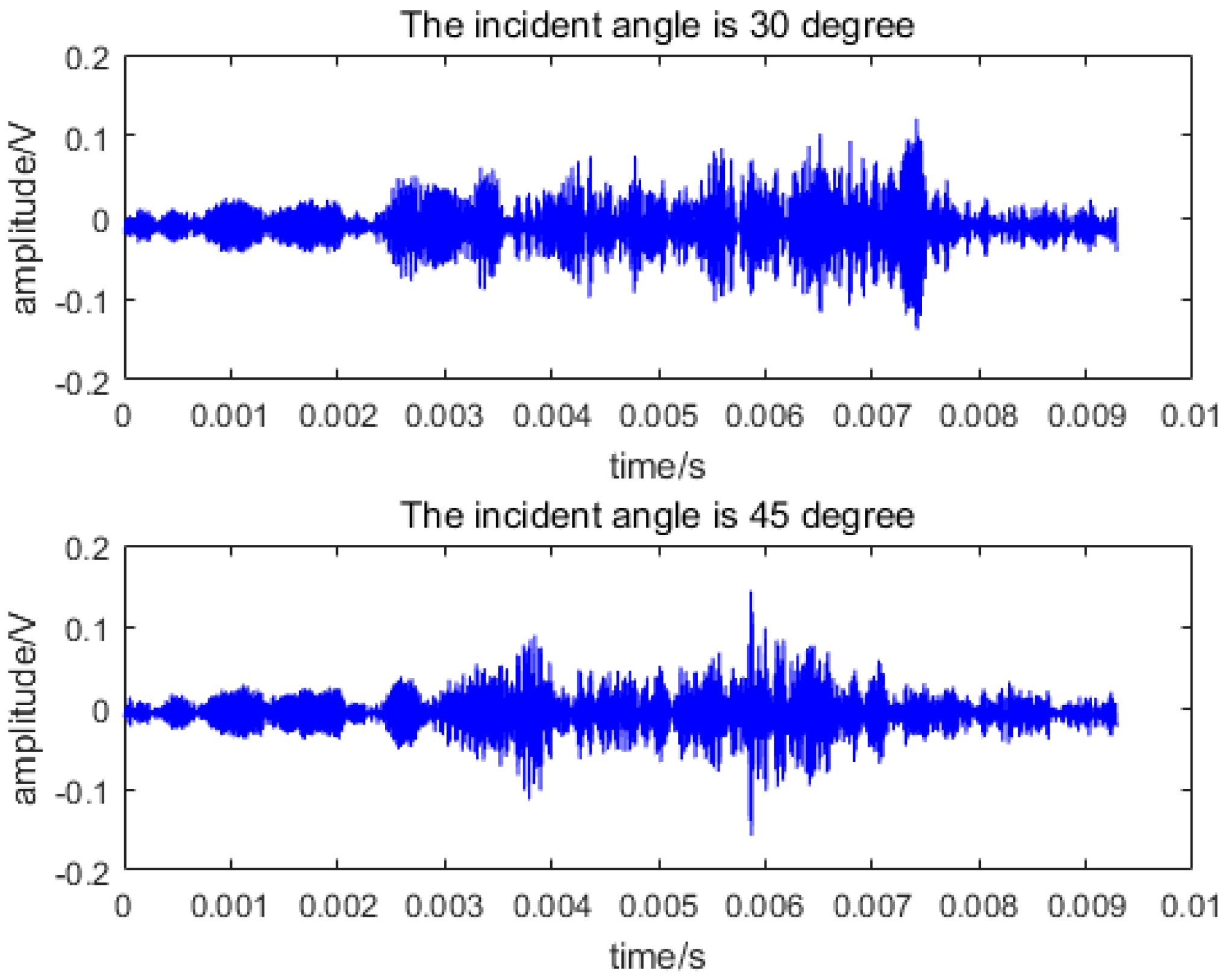
4.2. Simulation of Underwater Echo and Its Compression and Reconstruction

To verify the performance of the measurement matrix constructed with the proposed method, the highlight model [32] is used to simulate underwater echo, which is compressed and reconstructed by CS to evaluate the performance of the measurement matrix.
For an acoustic emission signal x ( t ) = x 0 ( t ) e j ω c t , in which ω c is the carrier frequency at 30 kHz, and x 0 ( t ) is the envelope assuming a trapezoidal shape. Assuming a sound velocity in fresh water of 1500 m/s and the pulse width is 10 ms. The number of points sampled is 4096. The underwater echo is simulated by the three-highlight model. Figure 3 shows the simulated echo with different signal-to-noise ratios (SNRs).
The simulated underwater echo in Figure 3 is then compressed and reconstructed with CS. In this study, the discrete cosine transform [33,34] is used as the sparse matrix, and the reconstruction algorithm adopted is the orthogonal matching pursuit (OMP) [35,36,37]. The measurement matrix based on the cyclic direct product and QR decomposition is compared respectively with Gaussian matrix, Bernoulli matrix, partial Hadamard matrix and Toeplitz matrix. The results are shown in Figure 4, Figure 5 and Figure 6.
As seen in the performance comparisons above, the signal compressed by the measurement matrix developed in this study provides better reconstruction results than those by other measurement matrices. Firstly, the SNR of the reconstructed signal is improved significantly. When the compression ratio is small, the performance of this matrix is nearly the same as other measurement matrices. As the compression ratio increases, our method shows greater improvement in the SNR. At a compression ratio of above 0.7, the SNR of this matrix is approximately 2 dB higher than those provided by other measurement matrices. In terms of the matching rate, the measurement matrix based on the cyclic direct product and QR decomposition yields higher reconstruction accuracy than the others, especially as the compression ratio increases.
Table 1 shows the construction time for various types of measurement matrices at different compression ratios.
As shown in the table, the measurement matrix based on the cyclic direct product and QR decomposition requires significantly less construction time than the others, as it only needs one two-dimensional matrix to be stored during construction, i.e., four elements. The storage space required is also less, as it is independent of the number of measurements made and only depends on the signal length N. The proposed measurement matrix thus saves storage space and computation time.

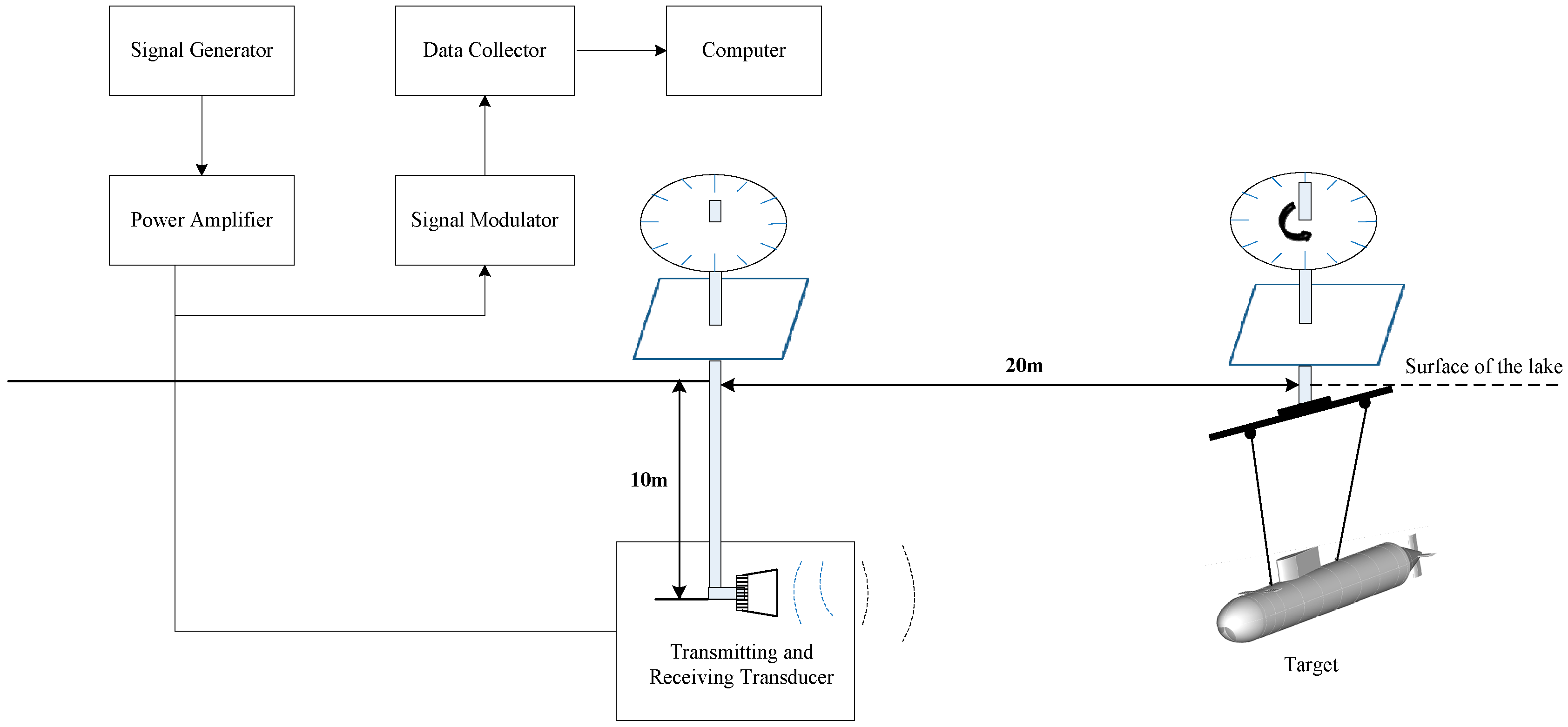
5. Testing the Performance of the Measurement Matrix Using Experimentally Measured Underwater Echo Data

The test was carried out at the experimental station of Qiandao Lake (Chunan, China). The test target was a scaled model of a submarine. The model is the Benchmark Target Strength Simulation Submarine (BeTSSi-Sub) manufactured by Dalian University of Technology. The deployment method is shown in Figure 7 [28].
The signal is emitted by the signal generator in the form of a Linear Frequency Modulation (LFM) signal with a frequency of 40 kHz–80 kHz, a pulse width of 1 ms, and a trigger interval of 200 ms. Through the power amplifier, an L6 linear power amplifier is used in the test, and its parameters adjusted according to the transducer’s working mode and impedance matching, with different gains; the underwater transducer uses a transmitting and receiving transducer through its internal transceiver conversion module; the transmission voltage response (TVR) is 162 dB and the receiving sensitivity is −172 dB. The output signal is then passed to the signal modulator and the LDS multi-channel data acquisition stage, with a sample frequency of 1 MHz. Finally, the signal is stored in the computer: this is the signal used in this paper.
There are two rotation stages, one for the transmitting/receiving transducer manufactured by the 726 institute in Shanghai, China (working at 40 kHz–80 kHz) and one for the rig holding the model submarine. They are 20 m apart, and both are 10 m underwater. In order to obtain echoes at different incident angles, the submarine model is rotated counterclockwise at uniform velocity.
Two typical angles, 30° and 45°, are selected for presentation of the measurements in this study. Figure 8 is the original echo signal obtained at incident angles of 30° and 45°. These signals are compressed and reconstructed by CS with Gaussian matrix, Bernoulli matrix, partial Hadamard matrix and Toeplitz matrix as the respective measurement matrix. The performance of the five types of measurement matrices is compared.
Figure 9 plots the changes in the SNR with the compression ratio.
The results processed from the experimentally measured data confirm the superior performance of the measurement matrix based on the cyclic direct product and QR decomposition in the processing of underwater echo, as compared to Gaussian matrix, Bernoulli matrix, partial Hadamard matrix and Toeplitz matrix. It provides greater enhancement in the SNR with increasing compression ratio. The partial Hadamard matrix is a deterministic measurement matrix, and is more effective for signal processing. However, it falls short on the length of the signal that it can process. This is overcome in the measurement matrix based on the cyclic direct product and QR decomposition, which also yields a better processing outcome than the other measurement matrices. Furthermore, the amount of data is also reduced, and the SNR is improved as anticipated.

6. Conclusions

Compressive Sensing overcomes the limitation of traditional sampling and provides a method to recover the original signal from a handful of non-adaptive nonlinear measurements. The measurement matrix is the key to this acquisition of data. As it is difficult to engineer a random measurement matrix, owing to the large storage space and complex computation required, and the deterministic measurement matrix is less satisfactory in terms of reconstruction accuracy, a measurement matrix constructed by the cyclic direct product and QR decomposition is proposed here. We tested its performance using simulated data and echoes from a scaled submarine target in a freshwater lake, at frequencies of 40 kHz–80 kHz. Gaussian matrix, Bernoulli matrix, partial Hadamard matrix, Toeplitz matrix and the measurement matrix proposed here are compared and analyzed in terms of their matching rate, SNR enhancement, and construction time, via signal compression and reconstruction. The measurement matrix based on the cyclic direct product and QR decomposition yields higher reconstruction accuracy than the others, especially as the compression ratio increases. In terms of SNR enhancement, performance is nearly the same as the other measurement matrices when the compression ratio is small. As the compression ratio increases, our method shows greater improvement in the SNR. At a compression ratio of above 0.7, the SNR of this matrix is approximately 2 dB higher than those provided by other measurement matrices. The proposed measurement matrix also requires significantly less construction time compared with the others, as it only needs one two-dimensional matrix to be stored during construction, i.e., four elements. The storage space required is less, as it is independent from the number of measurements made and only depends on the signal length. The proposed measurement matrix thus saves storage space and computation time.

Author Contributions

Conceptualization, Methodology, Validation, Writing—Original Draft Preparation, T.S. and H.C.; Writing—Review and Editing, P.B.; Formal Analysis, Y.G. and H.S.; Funding Acquisition, T.S., Y.G. and H.S.

Funding

This research was funded by the pre-research field fund project from Chinese Military Equipment Development Department, Grant No. 6140243010116DZ04001, the Extension Fund from Underwater Test and Control Technology Key Laboratory, Grant No. YS24071802 and Chinese National Natural Science Foundation, Grant Nos. 61871166 and 61703128.

Acknowledgments

This article uses experimental data collected at Dalian Test and Control Institute (China), and we gratefully acknowledge our colleagues for their experimental skills. T.S. worked on this article as a Visiting Research Fellow to the University of Bath (UK), thanks to the Chinese Scholarship Council (State Scholarship Fund No. 201608330338).

Conflicts of Interest

The authors declare no conflict of interest.

References

  1. Donoho, D.L.; Javanmard, A.; Montanari, A. Information-theoretically optimal compressed sensing via spatial coupling and approximate message passing. IEEE Trans. Inf. Theory 2013, 59, 7434–7464. [Google Scholar] [CrossRef]
  2. Candès, E.J.; Romberg, J.; Tao, T. Robust uncertainty principles: Exact signal reconstruction from highly incomplete frequency information. IEEE Trans. Inf. Theory 2006, 52, 489–509. [Google Scholar] [CrossRef]
  3. Candès, E.J.; Tao, T. Near-optimal signal recovery from random projections: Universal encoding strategies. IEEE Trans. Inf. Theory 2006, 52, 5406–5425. [Google Scholar] [CrossRef]
  4. Aksoylar, C.; Atia, G.K.; Saligrama, V. Sparse signal processing with linear and nonlinear observations: A unified shannon-theoretic approach. IEEE Trans. Inf. Theory 2017, 63, 749–776. [Google Scholar] [CrossRef]
  5. Lustig, M.; Donoho, D.; Pauly, J.M. Sparse MRI: The application of compressed sensing for rapid MR imaging. Magn. Reson. Med. 2007, 58, 1182–1195. [Google Scholar] [CrossRef] [PubMed] [Green Version]
  6. Huang, X.S.; Dai, Q.F.; Cao, Y.Q. Compressive sensing image fusion algorithm based on wavelet sparse basis. Appl. Res. Comput. 2012, 29, 3581–3583. [Google Scholar]
  7. Zhou, X.; Wang, W.; Liu, R.A. Compressive sensing image fusion algorithm based on direction lets. EURASIP J. Wirel. Commun. Netw. 2014, 1, 1–6. [Google Scholar]
  8. Wright, J.; Ma, Y.; Mairal, J. Sparse representation for computer vision and pattern recognition. Proc. IEEE 2010, 98, 1031–1044. [Google Scholar] [CrossRef]
  9. Wei, C.P.; Chen, C.F.; Wang, Y.C. Robust face recognition with structurally incoherent low-rank matrix decomposition. IEEE Trans. Image Process. 2014, 23, 3294–3307. [Google Scholar]
  10. Herman, M.A.; Strohmer, T. High-resolution radar via compressed sensing. IEEE Trans. Signal Process. 2008, 57, 2275–2284. [Google Scholar] [CrossRef]
  11. Wang, R.; Liu, G.; Kang, W.; Li, B.; Ma, R.; Zhu, C. Bayesian compressive sensing based optimized node selection scheme in underwater sensor networks. Sensors 2018, 18, 2568. [Google Scholar] [CrossRef]
  12. Hong, F.; Nian, W.; Quanbing, Z. Approach of image reconstruction based on sparse Bayesian learning. Chin. J. Image Graph. 2009, 14, 1064–1069. [Google Scholar]
  13. Boyali, A.; Kavakli, M. A robust gesture recognition algorithm based on sparse representation, random projections and compressed sensing. In Proceedings of the 2012 7th IEEE Conference on Industrial Electronics and Applications (ICIEA), Singapore, 18–20 July 2012; pp. 243–249. [Google Scholar]
  14. Mo, Q. A new method on deterministic construction of the measurement matrix in compressed sensing. arXiv, 2015; arXiv:1503.01250. [Google Scholar]
  15. Li, Z.L.; Chen, H.J.; Chang, Y. Compressed sensing reconstruction algorithm based on spectral projected gradient pursuit. Acta Autom. Sin. 2012, 38, 12–18. [Google Scholar] [CrossRef]
  16. Wang, R.; Zhang, J.; Ren, S. A reducing iteration orthogonal matching pursuit algorithm for compressive sensing. J. Tsinghua Univ. 2016, 21, 71–79. [Google Scholar] [CrossRef]
  17. Han, H.; Gan, L.; Liu, S. A novel measurement matrix based on regression model for block compressed sensing. J. Math. Imaging Vis. 2015, 51, 161–170. [Google Scholar] [CrossRef]
  18. Zhao, X.; Li, D. Improvement of Gauss random measurement matrix. Foreign Electron. Meas. Technol. 2017, 36, 25–29. [Google Scholar]
  19. Fang, H.; Zhang, Q.B. Method of image reconstruction based on very sparse random projection. Comput. Eng. Appl. 2007, 42, 25–27. [Google Scholar]
  20. Shaodong, L.I.; Yang, J.; Chen, W. Overview of radar imaging technique and application based on compressive sensing theory. J. Electron. Inf. Technol. 2016. [Google Scholar] [CrossRef]
  21. Boxue, H. Efficient recovery of block sparse signals by an improved algorithm of block-StOMP. J. Autom. 2017, 43, 1607–1618. [Google Scholar]
  22. Sun, J.M. Toeplitz matrix for compressed multipath channel sensing. Signal Process. 2012, 28, 879–885. [Google Scholar]
  23. Li, X.; Zhao, R.; Hu, S. Blocked polynomial deterministic matrix for compressed sensing. In Proceedings of the IEEE International Conference on Wireless Communications NETWORKING and Mobile Computing, Chengdu, China, 23–25 September 2010; pp. 1–4. [Google Scholar]
  24. Jia, T.; Chen, D.; Wang, J. Single-pixel color imaging method with a compressive sensing measurement matrix. Appl. Sci. 2018, 8, 1293. [Google Scholar] [CrossRef]
  25. Xiao, Y.; Gao, W.; Zhang, G. Compressed sensing based apple image measurement matrix selection. Int. J. Distrib. Sens. Netw. 2015, 11, 139–150. [Google Scholar] [CrossRef]
  26. Davenport, M.A.; Wakin, M.B. Analysis of Orthogonal Matching Pursuit Using the Restricted Isometry Property. IEEE Trans. Inf. Theory 2010, 56, 4395–4401. [Google Scholar] [CrossRef] [Green Version]
  27. Kou, N.; Li, L.; Tian, S. Measurement matrix analysis and radiation improvement of a metamaterial aperture antenna for coherent computational imaging. Appl. Sci. 2017, 7, 933. [Google Scholar] [CrossRef]
  28. Sun, T.J.; Blondel, P.; Jia, B.; Li, G.J.; Gao, E.W. Compressive sensing method to leverage prior information for submerged target echoes. J. Acoust. Soc. Am. 2018, 144, 1406–1415. [Google Scholar] [CrossRef] [PubMed]
  29. David, L.; Donoho, D.L. Compressed sensing. IEEE Trans. Inf. Theory 2006, 52, 1289–1306. [Google Scholar]
  30. Duarte, M.F.; Baraniuk, R.G. Kronecker compressive sensing. IEEE Trans. Image Process. 2012, 21, 494–504. [Google Scholar] [CrossRef]
  31. Lin, X.L.; Jiang, Y.L. QR decomposition and algorithm for unitary symmetric matrix. Chin. J. Comput. 2005, 5, 817–822. [Google Scholar]
  32. Chen, X.; Li, Y.A.; Dong, Z.C. Submarine echo simulation method based on the highlight model. In Proceedings of the 2013 IEEE International Conference of IEEE Region 10 (TENCON 2013), Xi’an, China, 22–25 October 2013; pp. 1–4. [Google Scholar]
  33. Chen, B.; Wang, H.X.; Cheng, L.Z. Fast directional discrete cosine transforms based image compression. J. Softw. 2011, 22, 826–832. [Google Scholar] [CrossRef]
  34. Hongxia, B.U. Compressed sensing SAR imaging based on sparse representation in fractional Fourier domain. Sci. China (Inf. Sci.) 2012, 55, 1789–1800. [Google Scholar]
  35. Sheng, C.; Jiawei, Z.; Dahang, F. Improved regularized orthogonal matching tracking DOA estimation method. Acoust. J. 2014, 1, 35–41. [Google Scholar]
  36. Dai, Y.; He, D.; Fang, Y. Accelerating 2D orthogonal matching pursuit algorithm on GPU. J. Supercomput. 2014, 69, 1363–1381. [Google Scholar] [CrossRef]
  37. Hussain, Z.; Shawe-Taylor, J.; Hardoon, D.R. Design and generalization analysis of orthogonal matching pursuit algorithms. IEEE Trans. Inf. Theory 2011, 57, 5326–5341. [Google Scholar] [CrossRef]
Figure 1. Compressive Sensing process of signal (a) compression of signal; (b) reconstruction of signal [28].
Applsci 08 02510 g001
Figure 2. Flowchart for the construction of the measurement matrix by the cyclic direct product and QR decomposition.
Applsci 08 02510 g002
Figure 3. Simulated echo signals with different signal-to-noise ratios.
Applsci 08 02510 g003
Figure 4. Reconstruction results by different types of measurement matrices (SNR = −3 dB).
Applsci 08 02510 g004
Figure 5. The matching rate comparison using different types of measurement matrices. (a) SNR = 4 dB; (b) SNR = 0 dB; (c) SNR = −3 dB.
Applsci 08 02510 g005aApplsci 08 02510 g005b
Figure 6. SNR enhancement comparison by different types of measurement matrices for different SNR (a) SNR = 4 dB; (b) SNR = 0 dB; (c) SNR = −3 dB.
Applsci 08 02510 g006aApplsci 08 02510 g006b
Figure 7. Deployment method in the test [28].
Applsci 08 02510 g007
Figure 8. Original echo signal.
Applsci 08 02510 g008
Figure 9. Change in SNR with the compression ratio. (a) echo with incident angle of 30°; (b) echo with incident angle of 45°.
Applsci 08 02510 g009
Table 1. Construction time for various types of measurement matrix at different compression ratios (t/s).
Compression RatioGaussian MatrixPartial Hadamard MatrixMatrix Based on Cyclic Direct Product and QR DecompositionBernoulli MatrixToeplitz Matrix
0.10.0940.0760.03740.0830.038
0.20.1160.1060.03870.1990.055
0.30.1900.1470.03980.2930.071
0.40.2180.1520.03990.3080.080
0.50.2370.1980.04140.5170.096
0.60.3170.2040.04210.6360.131

