Predicting Freeway Travel Time Using Multiple- Source Heterogeneous Data Integration

Abstract

Freeway travel time is influenced by many factors including traffic volume, adverse weather, accidents, traffic control, and so on. We employ the multiple source data-mining method to analyze freeway travel time. We collected toll data, weather data, traffic accident disposal logs, and other historical data from Freeway G5513 in Hunan Province, China. Using the Support Vector Machine (SVM), we proposed the travel time predicting model founded on these databases. The new SVM model can simulate the nonlinear relationship between travel time and those factors. In order to improve the precision of the SVM model, we applied the Artificial Fish Swarm algorithm to optimize the SVM model parameters, which include the kernel parameter σ, non-sensitive loss function parameter ε, and penalty parameter C. We compared the new optimized SVM model with the Back Propagation (BP) neural network and a common SVM model, using the historical data collected from freeway G5513. The results show that the accuracy of the optimized SVM model is 17.27% and 16.44% higher than those of the BP neural network model and the common SVM model, respectively.

1. Introduction

Travel time is one of the main indexes that reflect the traffic operation level of a freeway, and it is also the basis for Advanced Traveler Information System (ATIS), Traffic Guidance System (TGS), and Traffic Control System (TCS). Nowadays, large amount of heterogeneous data provides the new solution of travel time estimation. Meanwhile, semantic technology can deal with these complex, large-scale, and heterogeneous data. However, the challenges and difficulties of travel time prediction are identified below.

• Diverse influencing factors such as weather, holidays, traffic accidents, out of sample prediction, and mechanisms contributing to congestion. It is difficult to describe and predict the influence mechanism by using traditional conventional mathematical models.
• The complexity and incompleteness of basic data. Although many flow detectors and video detection equipment are on the freeway, captured data are incompatible, redundant, and include error or loss. To avoid these, techniques that use multi-source data to improve the accuracy of travel time prediction are extremely important.

In China, practical application of travel time prediction focuses mainly on the following two aspects.

The first aspect is the prediction of travel time by map navigation providers using their personalized GPS data. Many map service providers employ their personalized data for travel time forecast services and commercial products. For instance, Bai-du, Gao-de, and other Chinese map providers collect real-time GPS data from users while providing map navigation services. Then, a correlation algorithm is proposed to obtain the travel time prediction result at road sections, which depends on the market share of the map navigation service. As people use the navigation service with greater frequency, the GPS data will be more complete and the prediction accuracy will be higher. However, according to the Chinese market report, the market share of Bai-du and Gao-de services are presently 29.3% and 32.6%, respectively. Therefore, the accuracy of results should be further improved by increasing market share.

The second aspect is the prediction based on the traffic detection data of urban traffic managers and historical data. In recent years, numerous fixed detector devices have been installed in most urban roads and rural freeways to predict travel time; these devices include inductive loops, video recorder, microwave, and laser detectors. However, unavoidable damage to flow detection equipment and transmission error of partial data make traffic detection data incomplete, redundant, or incorrect. In addition, different detectors have different data formats and data accuracy. If the Traveler Information Service system uses inaccurate data, it cannot recommend optimal travel routes nor warn of potential traffic congestion, and users cannot determine optimal departure times nor estimate their arrival times.

Theoretical research on freeway travel time prediction can be divided into two categories based on single source data and multi-source data.

1.1. Overview of Prediction Method of Single Source Data

A single data source was an earlier method used to predict travel time. Many prediction results used in research were obtained using a single data source.

In 1997, Gipps [1] used occupancy and arrival time to predict travel time on a road. Mehmet and Nikolas [2] set statistical predictive algorithms to predict future travel time. Shen and Hadi [3] employed data obtained from freeway detectors. Kyung et al. [4,5] used inductive loop detectors to obtain the front position and capture interactions between trucks and non-trucks. However, fixed detector devices are easily influenced by the external environment and cannot directly access some important parameters, such as travel time, etc.

In addition, many researches consider using GPS data to predict travel time. Ramezani et al. [6] and Zhang et al. [7,8] considered the diversity of GPS data and investigated the application of Markov chain for travel time estimation and proved its accuracy. Woodard, Nogin & Paul et al. [9] used the GPS data from the current highest volume GPS data source and applied the TRIP method to predict travel time. Based on GPS data sets, Bahuleyan and Vanajakshi [10] proposed a prediction method for urban trunk lines that was only suitable for traffic conditions in India. GPS data only captures the sample vehicle speed and real-time position information and its’ accuracy depends greatly on the number of sample vehicles.

Clearly, these methods are innovations and improvements in travel time prediction, yielding more accurate results. However, many predictions that use a single data source do not consider the impact of other unexpected events, or the result was not accurate enough because a single data source cannot reflect the exact traffic state of a road network. It will result in certain errors between prediction results and true values.

1.2. Overview of Prediction Method of Multiple Source Data

Nowadays, traffic detector method and monitoring facilities have progressed rapidly. With the support of a large amount of data, it is possible to clearly visualize traffic flow changes under the joint action of different factors. Also, we can improve the adaptability and accuracy of traffic estimating model [11], and if the same state occurs, it can be predicted based on historical results. The more populated the database is, the higher the quality and the higher the likelihood of finding commonalities and predicting accurate results will be. This concept can be applied by searching for common traffic states prediction.

Owing to progress in the dynamic traffic information acquisition system, various traffic data can be collected more easily. Big data platform can integrate these different data sources, and apply the international standardized data description methods to facilitate data fusion and expansion. Data fusion can integrate the information of different data source and mine the useful hidden information from multiple data sources.

In data analysis, it is of great significance to mine the hidden semantic information in the data to assist in exploration. Ding et al. [12] converted the geographic coordinate information (latitude and longitude) in the data to street names to reflect the contextual semantic information. The trajectory of each taxi is regarded as a document composed of the street names passed by the taxi, and then introduced. Aldohuki et al. [13] proposed a new method, Semantic Traj, to manage and visualize taxi trajectory data in an intuitive, semantic-rich, and efficient manner.

Using multi-source data for prediction can overcome the limitations of the single data source. Semantic information in multi-source data can better describe the specific traffic flow state [14]. In other words, the single data source is of low quality and not comprehensive. The traffic state is described from different angles and directions to improve the accuracy of prediction and reduce disturbance from unexpected factors. The idea of data interoperability is used to facilitate the integration of data from different data sources, enabling multi-source data to be seamlessly linked as a single piece of data. The integration of data includes roads, directions, travel time, weather conditions, traffic accidents, holidays, etc.

Many studies have been conducted on travel time prediction, especially studies based on the historical data travel time from multi-source data.

Common prediction methods and their characteristics are summarized in

Table 1. Comparison of common prediction methods.

Prediction Method	Author	Data Source
Kalman filter	VanLint, J.W.C., 2006 [15]	Travel time data
	Zhou, J., 2014 [16]	Floating vehicle and fixed detector data
	Chang, T.H., 2016 [17]	Electronic Toll Collection (ETC) and traditional Vehicle Detector data
Bayesian estimation	Fei, X., 2011 [18]	The real loop detector data of an I-66 segment in Northern Virginia
	Zhan, X., 2016 [19]	A large-scale taxi trip dataset from New York City
Statistical decision theory	Wosyka, J., 2012 [20]	Two detectors data in Prague and also in the Czech Republic.
Neural network	Innamaa, S., 2005 [21]	Travel time data
	VanLint, J.W.C., 2005 [22]	Travel data and Some missing or corrupt travel data
Consolidated behaviormodels	Ben-Akiva, M., 2001 [23]	Origin-Destination flow data
	Mahmassani, H.C., 2001 [24]	O rigin-Destination trip information
	Chilà, G., 2016 [25]	The flow and the user’s behavior
	Alonso, B., 2017 [26]	Traffic loops and the signal control plans in Santander urban area

.

Compared to the single source data method, the multi-source data method can extract deep information within data, significantly reduce the cost of data acquisition, and make up for the lack of information and packet loss of single source data. At present, big data application technology are widely used in the traffic field, and many studies have been conducted in the field of freeway travel time prediction based on big data analytics. However, there are several deficiencies:

• The method pays attention to machine learning algorithms and does not consider the characteristics of the traffic flow, resulting in uncoordinated and unsuitable correspondence between the data and the traffic flow.
• As big data updates continuously, it provides conditions for traffic travel time prediction; however, some advantages and characteristics of these data are not captured, and a great deal of useful data are not being used and mined.
• Some model parameter calibrations are too subjective, which largely depends on the researchers’ experiences.
• Some models are too specific examples and cannot be easily adapted to other situations.

Therefore, in this study, we collected historical data from a freeway toll station. These data were categorized using the Semantic Technology (SVM) algorithm. In previous studies, Wu [27] used the support vector regression method to predict time; Vanajakshi [28] proposed one short-term prediction of travel time based on support vector. Using machine technology, Mendes-Moreira [29] obtained a regression method for comparing long-term travel time prediction through intelligent data analysis. However, their analysis is merely based on machine learning algorithms and does not improve the transportation system. The SVM model is not as sensitive to dirty data as the Kalman filter, resulting in unstable calculation of the filter parameters, and is not as vulnerable to dimensional catastrophe as other machine learning algorithms. Therefore, this paper uses the SVM model based on historical data to predict the common traffic state. Also, we simplified the method used for model construction. The practicability of the prediction algorithm was enhanced to overcome assumptions and uncertainties in the existing traffic flow theory. Through semantic technology, meteorological data, traffic records, and other field data are related.

2. Data Collection and Preprocessing

2.1. Data Description

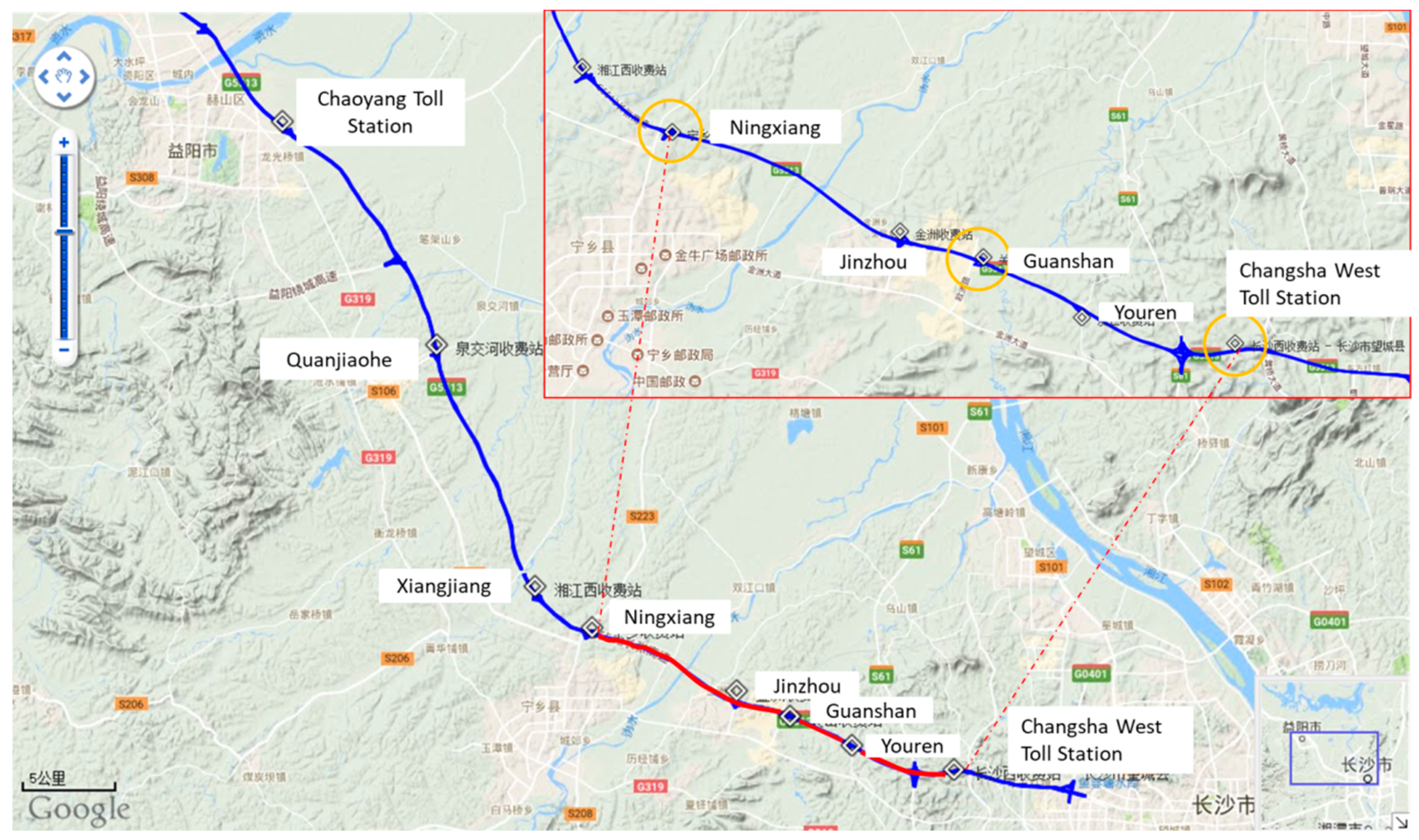
Data for this study was collected from Freeway G5513 that runs from Changsha to Yiyang, Hunan Province, starting from the Changsha toll station and ending at Yiyang toll station. This is a standard freeway with a two-way four lane speed of 100 km/h and a roadbed width of 26 m. The total length is approximately 63 km, the daily average flow reached 58,000 vehicles, and the peak flow during holiday or festival was up to 96,600 vehicles. Because of heavy traffic, the freeway has been rated as one of the six most congested sections in the Hunan Province. There are nine toll stations along the road, from east to west, which are Changsha West, Youren, Guanshan, Jinzhou, Ningxiang, Xiangjiang West, Quanjiao, Chaoyang, and YiyangNorth, illustrated in Figure 1.

The main data set collected in this study includes:

• Toll data of all toll stations along G5513 in February 2018 (vehicles entering and leaving toll station), with a total of 561,081 data items, including the name of the toll station, the time of vehicle entering and leaving the toll station, vehicle type and weight.
• Weather data of Meteorology monitoring stations, which was collected from the Chinese Weather Network in February 2018, with a total of 672 data items, including 24 h daily weather, temperature, relative humidity, precipitation, and wind direction.
• Freeway blockage record statistics, which was obtained from the freeway’s management department, a total of 260 freeway blockage information reports were collected in February, March, April, and May, including blockage location, reasons for the blockage, blockage start time, and blockage end time.
• Freeway traffic control measures report, which was obtained from the Traffic Police Department, with a total of seven data items collected on 5 April Qingming Traditional National Festival, May 1 International Labor Day, and other holiday control information.

2.2. Data Preprocessing

Many abnormal data items were found in the data, which need to be preprocessed before use.

● Data sharing the same entry and exit toll

On the freeway, some drivers turn around in the service area or other sections to avoid the charges and even exchange the toll tags, which is likely to make the entry and exit of the vehicles at toll stations consistent. Therefore, it is necessary to determine whether a data item is consistent with the toll gates and eliminate invalid data items.

● Abnormal time record data

If a toll station’s time system fails to synchronize or has a system failure, the time of accessing the toll station can be earlier than the time of exiting the toll station. In addition, there are other factors that can lead to long travel time, such as the breakdown of a vehicle on the road, accidents, and the situation where a driver may take a long rest in a service area. All of these situations will result in unusual time record data. During data preprocessing, abnormal time data records can be eliminated through screening.

● Missing data

There are two main reasons for missing data: on one hand, it can be caused by equipment problems or the road environment, including a detector’s unstable scanning frequency, faulty transmission equipment, and traffic jams; on the other hand, deleting unwanted data items may also erase accurate data. Lack of data will cause the road’s real traffic conditions to change directly or indirectly. Therefore, it is essential to make up for the missing data. Because of the strong continuity of the traffic flow travel time parameter, the trend in the change of the traffic flow travel time parameter with time is consistent, although its fluctuation will change as the collection period changes. Therefore, the following data fill formula is obtained, as given in Equation (1).

$$data\left(t\right)=\frac{2\mathrm{n}}{\mathrm{n}\left(\mathrm{n}+1\right)}\times data\left(t-1\right)+\frac{2\left(\mathrm{n}-1\right)}{\mathrm{n}\left(\mathrm{n}+1\right)}\times data\left(t-2\right)+\cdots +\frac{2}{\mathrm{n}\left(\mathrm{n}+1\right)}\times data\left(t-\mathrm{n}\right)$$

(1)

where, n is the number of data value taken to make up for missing data, data(t) represents the current missing data; data(t − 1), data(t − 2), and data(t − n) are the traffic flow travel time data of the past period, two cycles; and the n-th cycle are respectively represented. This method does not require the use of a historical database to extract historical trend data.

3. Support Vector Machine Model

3.1. Problem Descriptionof Freeway Travel Time Prediction

Freeway travel time is strongly consistent in a certain time range. That is, there are some complex functional relationships between the current travel time and the past travel time. By analyzing the changes in travel time, we can obtain rules and establish a real-time prediction model updated every five minutes. Then, the accuracy and reliability of the predicted results can be improved by using an optimization algorithm to find the optimal solution of the model.

The change in the freeway travel time in different time periods is not a simple linear relationship, and it will neither increase indefinitely, nor decrease indefinitely, but it will only change continuously within a floating interval. Therefore, using a simple least squares regression prediction or similar methods is not sufficient to predict the travel time. The SVM nonlinear regression theory can be employed to solve this problem.

SVM uses nonlinear transformation to map the original variables to a high-dimensional feature space so that the problem of nonlinear separability in the original sample space is transformed into high-dimensional feature space. The linear separable problem and the application of expansion theorem of the kernel function in the calculation process do not require the explicit expression of nonlinear mapping. In addition, since the linear learning machine is established in the high-dimensional feature space, it can be compared to the linear model. The comparison not only increases the complexity of the calculation, but also solves the problem of “dimensional disaster”.

Owing to changes in the traffic environment, sudden traffic accidents, weather, and other special events, the SVM algorithm will eventually be transformed into a quadratic programming problem. In theory, a global optimal solution can be obtained, thus solving the traditional neural network. The network can avoid the local optimal problem and should adequately accommodate the influencing factors caused by sudden changes to improve the accuracy of the travel time prediction result.

Therefore, this study used the nonlinear support vector machine regression theory [30].

3.2. Model Overview

The SVM is a machine learning method, which is based on the statistical learning theory developed by Vapnik. The theory has been further extended to diversified application algorithms, including the linear SVM classification algorithm, the nonlinear SVM classification algorithm, the linear SVM regression algorithm, and the nonlinear SVM regression algorithm [31]. These SVM algorithms have been widely used in many fields owing to their simple structure and high computational efficiency.

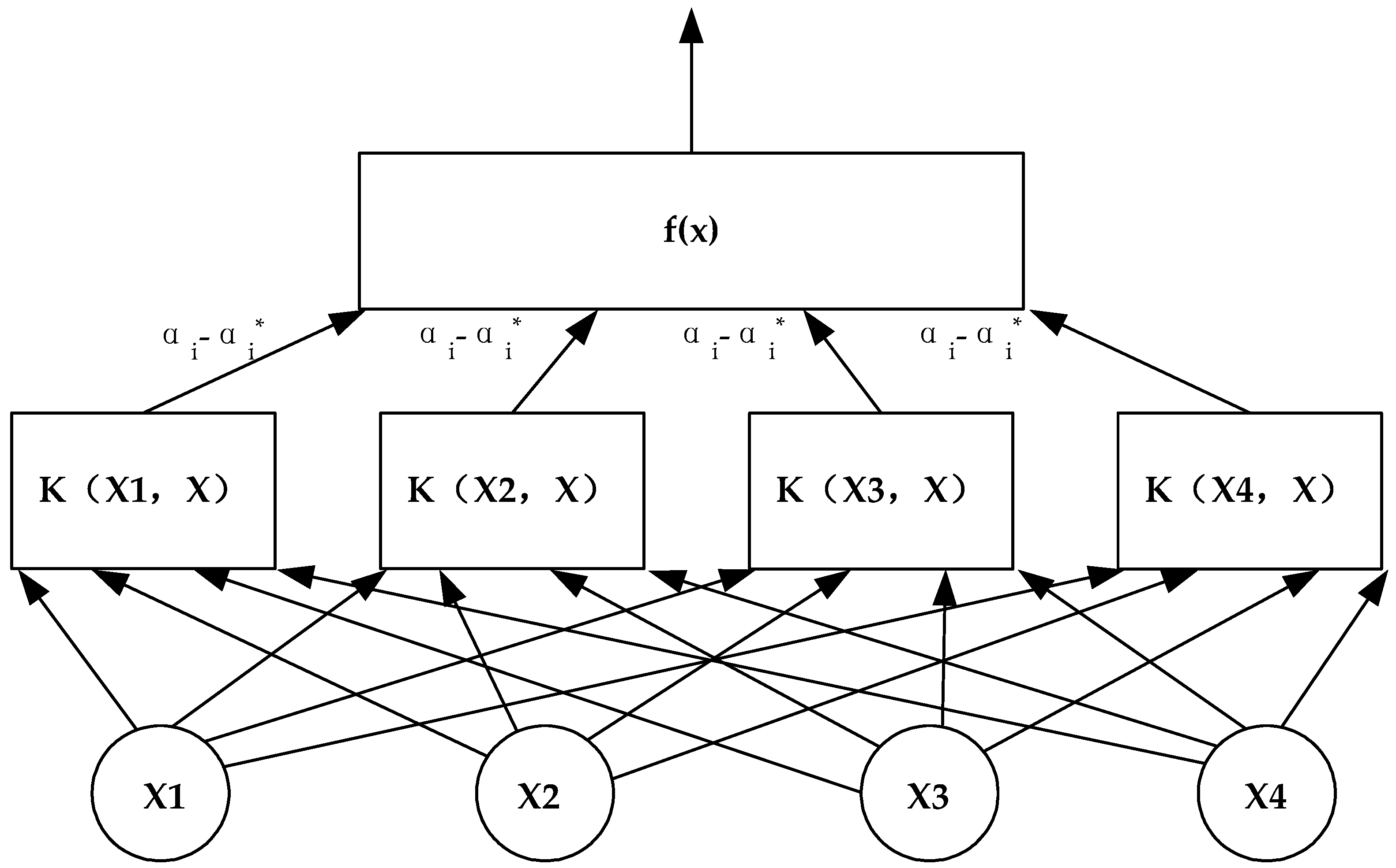
As in Figure 2, Consider a training sample set of $i$ training samples, $S = {\left\{\left(x_i,y_i\right)x_i\in R,y_i\in R\right\}}_{i=1}^l$, which is non-linear, where $x_i$ is the input column vector of the $i$ training sample, $x_i={\left[x_i^1,x_i^2\cdots ,x_i^d\right]}^T,y_i\in R$ is the corresponding output of the kernel function $K\left(x_i,y_i\right)=\partial {\left(x_i\right)}^T\ast \partial (x_j)$.

Equation (1) in the following is the linear regression equation established in the high dimensional space, and $\epsilon$ is introduced as a linear insensitive loss function:

$$f\left(x\right)=\omega \partial \left(x\right)+b$$

(2)

$$L\left(f\left(x\right),y,\epsilon \right)=\{\begin{array}{c}0,|f\left(x\right)-y|\le \epsilon \\ |f\left(x\right)-y|-\epsilon ,|f\left(x\right)-y|>\epsilon \end{array}$$

(3)

where, $\partial \left(x\right)$ is the nonlinear mapping function, $f\left(x\right)$ is the prediction function, which returns the predicted value, and y is the corresponding real value.

Under the above constraints, we can find the optimal classification hyper-plane, that is, find the solution to the following optimization problem.

$$\{\begin{array}{c}min\frac{{\Vert \omega \Vert }^2}{2}\\ s.t.\Vert {\omega }^T\partial \left(x_i\right)+b-y_i\Vert \le \epsilon ,i=1,2,\cdots ,l\end{array}$$

(4)

This problem can be solved by solving the saddle point of the Lagrange function, and its dual theory can be applied to solve the dual problem.

$$\{\begin{array}{c}min\frac{1}{2}{\displaystyle {\displaystyle \sum }_{i=1}^l}{\displaystyle {\displaystyle \sum }_{j=1}^l}\left({\alpha }_i-{\alpha }_i^{\ast }\right)({\alpha }_j-{\alpha }_j^{\ast })K\left(x_i,x_j\right)+\epsilon {\displaystyle {\displaystyle \sum }_{i=1}^l}\left({\alpha }_i-{\alpha }_i^{\ast }\right)-{\displaystyle {\displaystyle \sum }_{i=1}^l}{y}_i\left({\alpha }_i-{\alpha }_i^{\ast }\right)\\ s.t.{\displaystyle {\displaystyle \sum }_{i=1}^l}\left({\alpha }_i-{\alpha }_i^{\ast }\right)=0,{\alpha }_i^{\ast },{\alpha }_i\ge 0,i=1,2,\cdots ,l\end{array}$$

(5)

To solve the dual problem, a relaxation factor can be set for each data point. After introducing these two relaxation factors, ${\xi }_i,{\xi }_i^{\ast }({\xi }_i,{\xi }_i^{\ast }\ge 0,i=1,2,\cdots ,l)$, the function can be optimized as:

$$\{\begin{array}{c}min\frac{{\Vert \omega \Vert }^2}{2}+C{\displaystyle {\displaystyle \sum }_{i=1}^l}\left({\xi }_i-{\xi }_i^{\ast }\right)\\ s.t.{\omega }^T\partial \left(x_i\right)+b-y_i\le {\xi }_i+\epsilon ,i=1,2,\cdots ,l\\ s.t.y_i-{\omega }^T\partial \left(x_i\right)-b\le {\xi }_i^{\ast }+\epsilon ,i=1,2,\cdots ,l\end{array}$$

(6)

In the above equation, C is the penalty factor; the smaller the value, the smaller the penalty to the error data.

Next, the Lagrangian multiplier method can be used to solve the optimization algorithm, and the nonlinear regression function can be further used to solve the double optimization problem.

$$f\left(x\right)=\omega \partial \left(x\right)+b={\displaystyle \sum }_{i=1}^l\left({\alpha }_i-{\alpha }_i^{\ast }\right)\partial {\left(x_i\right)}^T\ast \partial \left(x_j\right)+b={\displaystyle \sum }_{i=1}^l\left({\alpha }_i-{\alpha }_i^{\ast }\right)K\left(x_i,y_i\right)+b$$

(7)

For the freeways, there is essentially no significant error in the travel time between the low peak period and even the flat peak period. However, the impact of different traffic conditions on travel time is inevitable during peak periods. Therefore, the two cases should be discussed separately. Furthermore, the weekday and weekend result in entirely different travel time on the highway. The commuting time, travel purpose, and travel mode will also be different. Therefore, these two points should be viewed separately. In addition, road weather conditions and traffic control will have certain influence on the prediction results and should be considered.

Based on the SVM model, input weekdays, weekends, the morning and evening peak periods, and off-peak hours as original values, we can obtain six time periods: the morning peak hours on weekdays, the evening peak hours on weekdays, off-peak hours on weekdays and so on. Weather and traffic control factors for the four scenarios can also be analyzed. However, the difference in highway traffic conditions between the weekday and the weekend, the morning and evening peak periods, and flat peak period is not considered due to the limitation of the length of the article.

This study used the travel time prediction of evening peak hours in the classified weekdays and weekend peak hours as an example by comparing the traffic data of multiple weekdays and weekends.

3.3. Model Construction

The freeway travel time prediction model is based on the SVM algorithm and is constructed based on the relationship between the current travel time of the road segment and the past travel time of the road segment, the current weather, and the possibility of traffic control.

In this study, we selected for analysis data from two toll stations with different distances from east to west of G5513. Moreover, because the passenger car accounts for the vast majority of the data, the travel time of the passenger car was taken as the prediction object.

In order to guarantee the uniformity of the multiple source data, time interval is set as five minutes.

Table 2. Toll station for travel time prediction.

Toll Station	Start Point	End Point	Distance (km)
1	Changsha West	Guanshan	10.6
2	Changsha West	Ningxiang	23.2

presents the characteristics of the toll stations.

The structure of the SVM is similar to the neural network. The output is a linear combination of intermediate nodes, and each intermediate node corresponds to a support vector. To determine the optimal classification function, this study takes the four travel times of the time period before the prediction time as the input, namely $t_{k-1}$, $t_{k-2}$, $t_{k-3}$, $t_{k-4}$.

$$t_k=g\left(t_{k-1},t_{k-2},t_{k-3},t_{k-4}\right)$$

(8)

k is the current time period, and $t_k$ represents the average travel time of all vehicles in the current predicted time period.

In the prediction process, due to the continuity of time, we can use the travel time to characterize the traffic flow, thus using the four travel times of the time period before the prediction time as the input. In addition, there are variables that can influence the predictions: weather, accidents that increases the travel time, holiday or non-holiday, and day of the week; as in

Table 3. Variables type and its meanings.

Variable Category	Variable Name	Variable Type	Variable Value	Variable Meaning
Meteorological	Weather status	Discrete	Clear; Cloudy; Fog; Overcast; Light rain; mod rain; hvy rain	Clear; Cloudy; Fog; Overcast; Light rain; mod rain; hvy rain
Time	Holiday	Discrete	0	N
			1	Y
	Weekday	Discrete	1 … 7	Monday … Sunday
Accident	Traffic accidents	Discrete	0	N
			1	Y

:

Many traffic accidents occur on the freeway every day. To simplify the parameters, we divide traffic accidents into two categories: traffic accidents that increase travel time and those that do not. In this study, traffic accidents were regarded as invariant.

Figure 3 shows a comparison of travel time increased by an accident with normal travel time on the afternoon of 17 February.

Since SVM is a machine learning model, sample training is required before prediction. Multiple groups of any four consecutive travel times, daily weather, traffic accidents that increase the travel time, holidays, and weekday data were used as training samples to obtain a trained model. In the trained model, $t_{k-1}$, $t_{k-2}$, $t_{k-3}$, $t_{k-4}$, weather, accident, holiday, and week are used to predict the travel time of the next time period. When a certain number of training samples is achieved, real-time data input can be adopted to predict future results. Moreover, the model can be constantly modified based on the relation between the predicted data and the predicted data to prediction accuracy.

3.4. Parameter Calibration and Optimization

Parameter selection is very important to find the optimal hyper-plane in the SVM model used in this study. The insensitive loss function parameter ε decides the permitted error of function. Therefore, a proper value of ε is much needed according to the actual demand, and the penalty parameter C, which is also called Upper Bound, which denotes the upper bound function. However, existing studies mainly adopted the traditional grid search method, direct determination method, one-dimensional search method, and inverse ratio method to determine the insensitive loss function parameter ε and penalty parameter C. However, there are many shortcomings associated with these methods, and the resulting errors will significantly influence the accuracy of the prediction results.

Moreover, in the SVM model, kernel function selection is also an important factor that influences the performance of the SVM. The radial basis kernel function $K\left(x_i,y_i\right)=e^{\frac{\Vert x-x_i\Vert }{{\sigma }^2}}$ (RBF) is an adaptive kernel function for low-dimensional space data and high-dimensional space, which have good convergence domains, and this function can be described as an ideal kernel function. Therefore, the RBF was selected as the classification prediction kernel function of the SVM, in which a kernel parameter σ needs to be optimized.

Therefore, three parameters need to be optimized, namely the core parameter σ, the non-sensitive loss function parameter ε, and the punishment parameter C. The kernel parameter σ is the distribution or range of the training sample data. The non-sensitive loss function parameter ε affects the number of support vectors. The larger the value of ε, the lower the regression precision, and the fewer the support vectors. The penalty parameter C is used to control the degree of punishment of samples beyond the allowable error range. The higher the value, the heavier the punishment of samples.

We used the artificial fish swarm algorithm to optimize the parameters of the regression model. The artificial fish swarm algorithm has unique advantages in parameter optimization and overcomes the blindness of traditional algorithms in parameter optimization and the defects of the linear model and neural network in parameter selection. It can be said that the parallel performance of the artificial fish swarm algorithm can ensure that the model parameters converge faster to the global optimization extreme [32].

4. Case Study

4.1. Data Selection

The data used in this study was collected in February 2018 on G5513 (from Changsha West to Guanshan/Ningxiang Station) in Changsha, Hunan Province, China. The travel time was detected for all days and the detection interval was five minutes. Furthermore, 288 sequences are included in one day.

The daily evening peak (17:00–19:00) data from G5513 (Changsha West to Guanshan/Ningxiang Station) was selected as a sample after comparing data of multiple weekdays and weekends, which contains 204 to 228 items. Other variable data items also need to be filtered according to the data above. The dimension feature values are based on the time series and the data requirements according to the prediction model.

In this study, the regression SVM model is used to establish the model parameters, and the artificial fish swarm algorithm is used to establish the model parameter optimization algorithm. The first step in the optimization process of the artificial fish swarm algorithm is to feed in the training value and the training target through the SVM model to calculate the fitness of the individual. The most adaptable individual is regarded as the optimal value of the current fish group and the corresponding parameters σ, ε, and C of the current optimal value are saved. In the subsequent iteration, σ, ε, and C corresponding to the maximum fitness value are taken as the final optimization results. According to the result of the optimization, all kernel function, loss function, and penalty parameters could be adjusted to look for the best SVM model for the prediction. The optimization results are presented in

Table 4. Optimization of parameter values.

Section	Penalty Parameter, C	Nuclear Parameter, σ	Insensitive Loss Function Parameter, ε
Changsha West–Guanshan	6.8755	0.0064	0.3461
Changsha West–Ningxiang	8.6485	0.0034	0.6991

. The optimization process for the optimal value of the penalty parameter C is shown in Figure 4.

The parameters of the artificial fish swarm algorithm are set as follows: the maximum number of iterations of the artificial fish is 100; the population size is 5; the maximum number of trials is 5; the crowding factor δ is 0.618; the perceived distance is 0.5; and the moving step is 0.1.

4.2. Results and Comparative Analysis

The data adopted in this study were obtained during the Chinese Spring Festival from 15 to 21 February 2018.Therefore, the data were divided into weekdays and holidays. There were 336 sets of data from 1 to 14 February 2018 (14 days data) in each group of toll stations; 264 groups (11 days) were randomly selected as training data input, and 72 groups (3 days) were adopted as prediction numbers. There were 168 sets of data from 15 to 21 February 2018 (11 days data) in each group of toll stations; 96 groups (4 days) were randomly selected as training data input, and 72 groups (3 days) were adopted as prediction numbers.

The detection time is from 17:00 to 19:00, and the value was taken as test data.

BP neural network, SVM, and optimized SVM were used for the prediction. The root mean square error (RMSE), the mean absolute percent error (MAPE) and the covariance protocol (CP) were selected as the error evaluation criteria in the prediction process [33]. The RMSE is a comprehensive evaluation indicator of the prediction effect, the MAPE is the prediction relative error, while the CP is the error component analysis indicator.

Figure 5 show the forecasting effect diagram of the holiday evening peak.

From

Table 5. Error evaluation of forecasting freeway travel time.

	Method	Changsha West–Guanshan Station				Changsha West–Ningxiang Station
		RMSE	L-RMSE	MAPE	CP	RMSE	L-RMSE	MAPE	CP
Weekday	BPNN	7.6544	9.3541	5.0873	0.5489	10.5124	11.9621	5.5104	0.5809
	SVM	6.3405	8.3952	4.8225	0.5810	9.0375	11.6215	4.5422	0.6930
	OSVM	6.0369	8.0369	4.6536	0.5952	8.3069	10.6541	4.4524	0.6404
Weekend	BPNN	11.6308	13.6169	9.1023	0.5990	16.0845	16.9551	9.6148	0.6454
	SVM	11.5152	13.1510	7.8645	0.6460	13.3215	14.4151	8.1153	0.6905
	OSVM	9.6218	11.7411	6.2451	0.7621	12.2548	15.0215	7.8651	0.7245

BPNN: BP Neural Network; SVM: Support Vector Machine; OSVM: Optimized SVM; L-RMSE: an RMSE that lacks multi-source data and uses only past data for prediction.

, one can observe that the weekday was predicted by the RMSE, the MAPE, and the CP data between the two toll stations. It appears that all three models can be used for predicting travel time.

Although the prediction error of the BP neural network may be larger than those of the SVM and the optimized SVM models, there is no deviation between the error of the SVM and the optimized SVM model.

However, when forecasting holidays with heavy traffic and long travel times, the RMSE of the optimized SVM model is significantly better than those of the BP neural network and the SVM model.

In the prediction of Changsha West–Guanshan, the accuracy of the optimized SVM model using artificial fish swarm algorithm is 17.27% higher than that of the BP neural network model and 16.44% higher than the conventional SVM model.

In the prediction of Changsha West–Ningxiang, the accuracy of the optimized SVM model using artificial fish swarm algorithm is 23.80% and 8.01% higher than those of the BP neural network model and the conventional SVM model, respectively.

The RMSE lacking multi-source data was added to compare with the normal RMSE. Compared with BP neural network and SVM algorithm, it can be clearly seen that SVM has proved to be a highly accurate method in traffic data fusion. Therefore, the optimized SVM multi-source traffic data quality control model is feasible and effective. This means that the optimized SVM model described in this paper has higher travel time prediction accuracy in the road segment, and the mapping law of the input and output are better represented by the optimized SVM model.

In terms of the relative prediction errors of the three prediction models, the MAPE of the optimized SVM model is lower than the prediction errors of the BP neural network and the conventional SVM model when using holiday and weekday data. This indicates that the optimized SVM model described in this paper has certain advantages in terms of the travel time prediction model of the road segment, and the data requirements are lower.

4.3. Analysis of Influencing Factors of Travel Time

Freeway travel time is determined by various factors, such as weather, traffic accidents, holidays, and weekdays. However, owing to limitations of the sample data, only traffic accidents and holidays were considered in this paper.

4.3.1. Effect of Traffic Accidents on Travel Time

In order to reveal the effect of accidents on travel time, we used the BP, SVM, and the optimized SVM model to predict travel time from Changsha toll station to Guanshan toll station on G5513. One traffic accident took place at 15:40 and ended at 16:34 on 7th February 2018. The accident site located between these two toll stations. Travel time is listed in Figure 6, which includes the actual value, BP prediction value, SVM, and optimized SVM prediction value.

From Figure 6, travel time increased by 70% at 16:00 (from 50 min to 85 min), and increased by 230% at 17:00 (up to 165 min). The figure indicates that accident can influence travel time greatly.

The prediction results also indicate that the optimized SVM model is superior to the BP neural network and SVM model in terms of the CP. In the prediction of Changsha West–Guanshan, the CP of the optimized SVM model is higher than those of BP model and SVM model by 21.40% and 7.28% respectively. In the prediction of Changsha West–Ningxiang, the CP of the optimized SVM model is higher than those of BP model and SVM model by 10.9% and 6.53%, respectively. The results proved that the optimized SVM model has better inclusiveness and stability when unexpected factors such as traffic accidents, thereby avoiding the need for repeated trial and error to address network problems.

4.3.2. Effect of Holidays on Travel Time

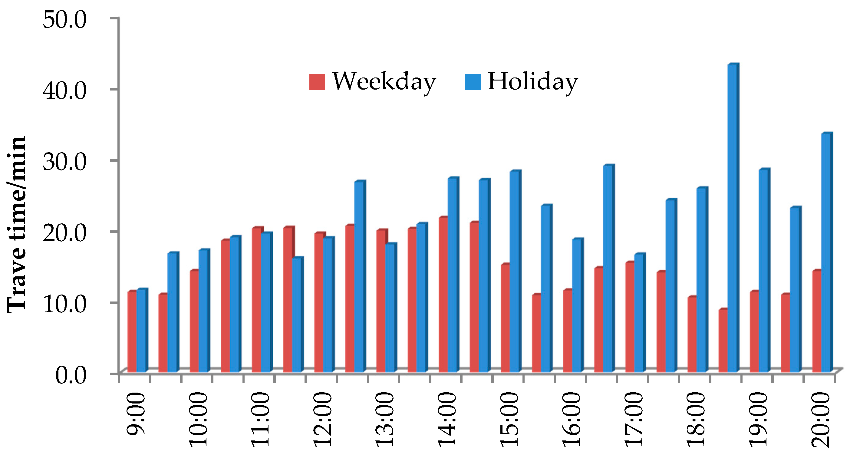
In this section, we compared travel time on holiday (21 February) with that on weekday (13 February). The study range is from Changsha toll station to Guanshan toll station on G5513. Travel time was analyzed from 9:00 to 20:00. Results of weekday and holiday are shown in Figure 7.

From Figure 7, travel time on holiday is basically longer than that on weekday. This trend is more significant in the afternoon. For example, holiday travel time can double weekday travel time at 15:00 to 20:00.

From above, we can observe that holidays have significant influence on travel time. On weekdays, traffic flow on G5513 is an average of 64,000 vehicles per day. In comparison, traffic flow will reach 93,000 vehicles per day on holidays (for example, Chinese Spring Festival), which is 1.6 times of the weekday.

Also, a comparison of the weekday and holiday forecasting error evaluation criteria presented in the previous section indicates that the BP neural network has a greater prediction error than the weekday prediction results of the other models, probably due to the problem of building the network structure. However, the conventional SVM and the optimized SVM models have similar prediction error results. In the above analysis, there are large gaps in the holiday prediction results of the three different models, but whether it is on weekdays or holidays, the prediction accuracy of the optimized SVM model described in this paper is more accurate.

5. Conclusions

This study performed an in-depth analysis of freeway travel time prediction to provide a high-quality travel experience for users. We found that freeway travel time is increased by holiday, weather, accident and traffic. We analyzed the effect of different factors, such as accidents and holidays, by removing the effects of accidents and traffic through data integration and comparing them with original data.

Bad weather reduces the overall traffic rate, which increases the travel time. Traffic accidents lead to reduced road traffic capacity, which increases the travel time. Free passage on highways during holidays and the increased demand for travel result in increased vehicle flow, which also increases the travel time.

In this study, we analyzed basic data and proposed to base the traffic state prediction method on SVM data mining technology. This transformed the problem into a quadratic programming problem using the artificial fish swarm algorithm, which reduces the computational and local optimal problems of traditional neural networks. The parameters of the SVM were optimized using traditional network optimization, and a global optimal solution was obtained. Results show that the accuracy of the optimized SVM model is 17.27% and 16.44% higher than those of the BP neural network model and the conventional SVM model, respectively. Accurate prediction of freeway travel time was realized, which can provide data support for monitoring, early warning, and decision analysis for the freeway operation status.

In this study, influencing factors such as weather, traffic, accidents and holidays were included in the optimization of the SVM prediction model. However, owing to limitations of the number of samples, the model was not fully trained. Therefore, a certain error occurred in the prediction results.

In the future, it will be necessary to categorize traffic accidents, clarify the impact of each type of accident on the travel time, categorize the increase in holiday traffic, and clarify the impact of each level of accident on the travel time. Furthermore, the number of training samples, database capacity, and prediction accuracy should be continuously increased. In this study, only data from freeway toll stations were validated; application to actual large-scale road networks should be further explored in the future.

References

- Gipps, P.G. The Estimation of a Measure of Vehicle Delay from Detector Output; Newcastle-Upon-Tyne University: Northumberland, UK, 1977; pp. 1–18. [Google Scholar]
- Yildirimoglu, M.; Geroliminis, N. Experienced travel time prediction for congested freeways. Transp. Res. Part B Method 2013, 53, 45–63. [Google Scholar] [CrossRef] [Green Version]
- Shen, L.; Hadi, M. Practical approach for travel time estimation from point traffic detector data. J. Adv. Transp. 2013, 47, 526–535. [Google Scholar] [CrossRef]
- Hyun, K.; Tok, A.; Ritchie, S.G. Long distance truck tracking from advanced point detectors using a selective weighted Bayesian model. Transp. Res. Part C Emerg. Technol. 2016, 82, 24–42. [Google Scholar] [CrossRef]
- Hyun, K.K.; Jeong, K. Assessing crash risk considering vehicle interactions with trucks using point detector data. Accid. Anal. Prev. 2018. [Google Scholar] [CrossRef] [PubMed]
- Ramezani, M.; Geroliminis, N. On the estimation of arterial route travel time distribution with Markov chains. Transp. Res. Part B 2012, 46, 1576–1590. [Google Scholar] [CrossRef] [Green Version]
- Zhang, J.T.; Zhou, J. An Arterial Travel Time Estimation Model Based on Discrete Time Markov Chains. Syst. Eng. 2014, 5, 98–104. [Google Scholar] [CrossRef]
- Zhang, J.T.; Zhou, J. Travel time estimation model based on spatial Markov chains. Syst. Eng. 2015, 12, 72–77. [Google Scholar]
- Woodard, D.; Nogin, G. Predicting travel time reliability using mobile phone GPS data. Transp. Res. Part C Emerg. Technol. 2017, 75, 30–44. [Google Scholar] [CrossRef]
- Bahuleyan, H.; Vanajakshi, L.D. Arterial path-level travel-time estimation using machine-learning techniques. J. Comput. Civ. Eng. 2016, 31, 04016070. [Google Scholar] [CrossRef]
- Zhou, X.; Liu, Z.; Zhao, X.X.; Guo, J.H. Framework for dynamic od matrix estimation based on multi-source traffic data fusion. Appl. Mech. Mater. 2014, 505–506, 1153–1156. [Google Scholar] [CrossRef]
- Chu, D.; Sheets, D.A.; Zhao, Y.; Wu, Y.; Zheng, M.; Chen, G.; Yang, J. Visualizing hidden themes of Taxi Movement with semantic transformation. In Proceedings of the 2014 IEEE Pacific Visualization Symposium, Yokohama, Kanagawa, Japan, 4–7 March 2014; IEEE Computer Society Press: Los Alamitos, CA, USA, 2014; pp. 137–144. [Google Scholar]
- Al-Dohuki, S.; Wu, Y.; Kamw, F. Semantic Traj: A new approach to interacting with massive taxi trajectories. IEEE Trans. Vis. Comput. Gr. 2017, 23, 11–20. [Google Scholar] [CrossRef] [PubMed]
- Lécué, F.; Tallevi-Diotallevi, S.; Hayes, J.; Tucker, R.; Bicer, V.; Sbodio, M.; Tommasi, P. Smart traffic analytics in the semantic web with STAR-CITY: Scenarios, system and lessons learned in Dublin City. J. Web Semant. 2014, 27–28, 26–33. [Google Scholar] [CrossRef]
- vanLint, J.W.C. Incremental and online learning through extended kalman filtering with constraint weights for freeway travel time prediction. In Proceedings of the 2006 IEEE Intelligent Transportation Systems Conference, Toronto, ON, Canada, 17–20 September 2006; pp. 1041–1046. [Google Scholar]
- Zhou, J.; Zhang, C.B. Travel Time Prediction Model for Urban Road Network based on Multi-source Data. Procedia Soc. Behav. Sci. 2014, 138, 811–818. [Google Scholar]
- Chang, T.H.; Chen, A.Y.; Hsu, Y.T.; Yang, C.L. Freeway Travel Time Prediction Based on Seamless Spatio-temporal Data Fusion: Case Study of the Freeway in Taiwan. Transp. Res. Procedia 2016, 17, 452–459. [Google Scholar] [CrossRef]
- Fei, X.; Lu, C.C. A Bayesian dynamic linear model approach for real-time short-term freeway travel time prediction. Transp. Res. Part C 2011, 19, 1306–1318. [Google Scholar] [CrossRef]
- Zhan, X.; Ukkusuri, S.V. A Bayesian mixture model for short-term average link travel time estimation using large-scale limited information trip-based data. Autom. Constr. 2016, 72, 237–246. [Google Scholar] [CrossRef]
- Wosyka, J.; Pribyl, P. Real-time travel time estimation on highways using loop detector data and license plate recognition. In Proceedings of the 2012 Elektro, Žilina-Rajecké Teplice, Slovakia, 21–22 May 2012; pp. 391–394. [Google Scholar]
- Innamaa, S. Short-Term Prediction of Travel Time using Neural Networks on an Interurban Highway. Transportation 2005, 32, 649–669. [Google Scholar] [CrossRef]
- vanLint, J.W.C.; Hoogendoorn, S.P. Accurate freeway travel time prediction with state-space neural networks under missing data. Transp. Res. Part C 2005, 13, 347–369. [Google Scholar] [CrossRef]
- Ben-Akiva, M.; Bierlaire, M.; Burton, D.; Koutsopoulos, H.N.; Mishalani, R. Network State Estimation and Prediction for Real-Time Traffic Management. Netw. Spat. Econ. 2001, 1, 293–318. [Google Scholar] [CrossRef]
- Mahmassani, H.S. Dynamic Network Traffic Assignment and Simulation Methodology for Advanced System Management Applications. Netw. Spat. Econ. 2001, 1, 267–292. [Google Scholar] [CrossRef]
- Chilà, G.; Musolino, G.; Polimeni, A.; Rindone, C.; Russo, F.; Vitetta, A. Transport models and intelligent transportation system to support urban evacuation planning process. IETIntell. Transp. Syst. 2016, 10, 279–286. [Google Scholar]
- Alonso, B.; Pòrtilla, Á.I.; Musolino, G.; Rindone, C.; Vitetta, A. Network Fundamental Diagram (NFD) and traffic signal control: First empirical evidences from the city of Santander. Transp. Res. Procedia 2017, 27, 27–34. [Google Scholar] [CrossRef]
- Wu, C.H.; Ho, J.M. Travel-time prediction with support vector regression. IEEE Trans. Intell. Transp. Syst. 2004, 5, 276–281. [Google Scholar] [CrossRef]
- Vanajakshi, L.; Rilett, L.R. Support Vector Machine Technique for the Short-Term Prediction of Travel Time. In Proceedings of the 2007 IEEE Intelligent Vehicles Symposium, Istanbul, Turkey, 13–15 June 2007; pp. 600–605. [Google Scholar]
- Mendes-Moreira, J.; Jorge, A.M.; de Sousa, J.F.; Soares, C. Comparing state-of-the-art regression methods for long term travel time prediction. Intell. Data Anal. 2012, 16, 427–449. [Google Scholar] [CrossRef]
- Wang, X.; Chen, X.H.; Yang, X.M. Short term prediction of expressway travel time based on k nearest neighbor algorithm. Chin. J. Highw. Transp. 2015, 28, 102–111. [Google Scholar]
- Li, S.; Yuan, Z.C.; Wang, C. Optimization of support vector machine parameters based on group intelligence algorithm. CAAI TIS 2018, 13, 70–84. [Google Scholar]
- Wang, Q.; Liu, Z.; Peng, Z. A PSO-SVM Model for short-term travel time prediction based on Bluetooth Technology. J. Harbin Inst. Technol. 2015, 22, 7–14. [Google Scholar]
- Yang, Z.S. Study on the Synthetic Link Travel Time Prediction Model of Key Theory of ITS. J. Traffic Transp. Eng. 2001, 1, 65–67. [Google Scholar]
Figure 1.
Layout of Freeway G5513 and toll stations.
Figure 2.
Structure of Support Vector Machine (SVM) model.
Figure 3.
Comparison of accidents and normal travel time.
Figure 4.
The parameter optimization curve.
Figure 5.
Results of freeway travel time prediction.
Figure 6.
Travel time during traffic accident.
Figure 7.
Comparison of weekday and holiday.