Research on a Mixed Gas Classification Algorithm Based on Extreme Random Tree

1
School of Electrical Engineering and Automation, Harbin Institute of Technology, Harbin 150001, China
2
School of Measurement and Control Technology and Communication Engineering, Harbin University of Science and Technology, Harbin 150001, China
*
Author to whom correspondence should be addressed.
Appl. Sci. 2019, 9(9), 1728; https://doi.org/10.3390/app9091728
Submission received: 26 March 2019
/
Revised: 24 April 2019
/
Accepted: 24 April 2019
/
Published: 26 April 2019
(This article belongs to the Section Computing and Artificial Intelligence)
Abstract
:Because of the low accuracy of the current machine olfactory algorithms in detecting two mixed gases, this study proposes a hybrid gas detection algorithm based on an extreme random tree to greatly improve the classification accuracy and time efficiency. The method mainly uses the dynamic time warping algorithm (DTW) to perform data pre-processing and then extracts the gas characteristics from gas signals at different concentrations by applying a principal component analysis (PCA). Finally, the model is established by using a new extreme random tree algorithm to achieve the target gas classification. The sample data collected by the experiment was verified by comparison experiments with the proposed algorithm. The analysis results show that the proposed DTW algorithm improves the gas classification accuracy by 26.87%. Compared with the random forest algorithm, extreme gradient boosting (XGBoost) algorithm and gradient boosting decision tree (GBDT) algorithm, the accuracy rate increased by 4.53%, 5.11% and 8.10%, respectively, reaching 99.28%. In terms of the time efficiency of the algorithms, the actual runtime of the extreme random tree algorithm is 66.85%, 90.27%, and 81.61% lower than that of the random forest algorithm, XGBoost algorithm, and GBDT algorithm, respectively, reaching 103.2568 s.
1. Introduction
In the development of electronic technology and artificial intelligence, sensing applications and machine learning algorithms are becoming increasingly intelligent, which promotes the continuous development of machine olfaction. This introduction will briefly place this study in a broad context and highlight why it is important. Machine olfaction is a new type of biomimetic detection technology, which can be used to simulate the working mechanism of biological olfaction. It is often used in the analysis and detection of various gases, such as in pollution control [1,2], medical technology [3,4], and oil exploration [5]. Researchers have achieved good results in the study of machine olfaction [6,7,8]. In the area of this research, the detection of dangerous flammable and explosive gases is particularly important, and the safety problems caused by gas leakage are prevalent all over the world, which seriously endangers human life [9]. If these gases can be detected, classified and identified timeously and the leakage situation and trend can be determined, the occurrence of dangerous accidents can be avoided to a large extent. Therefore, the detection of flammable and explosive toxic gases is of great significance.
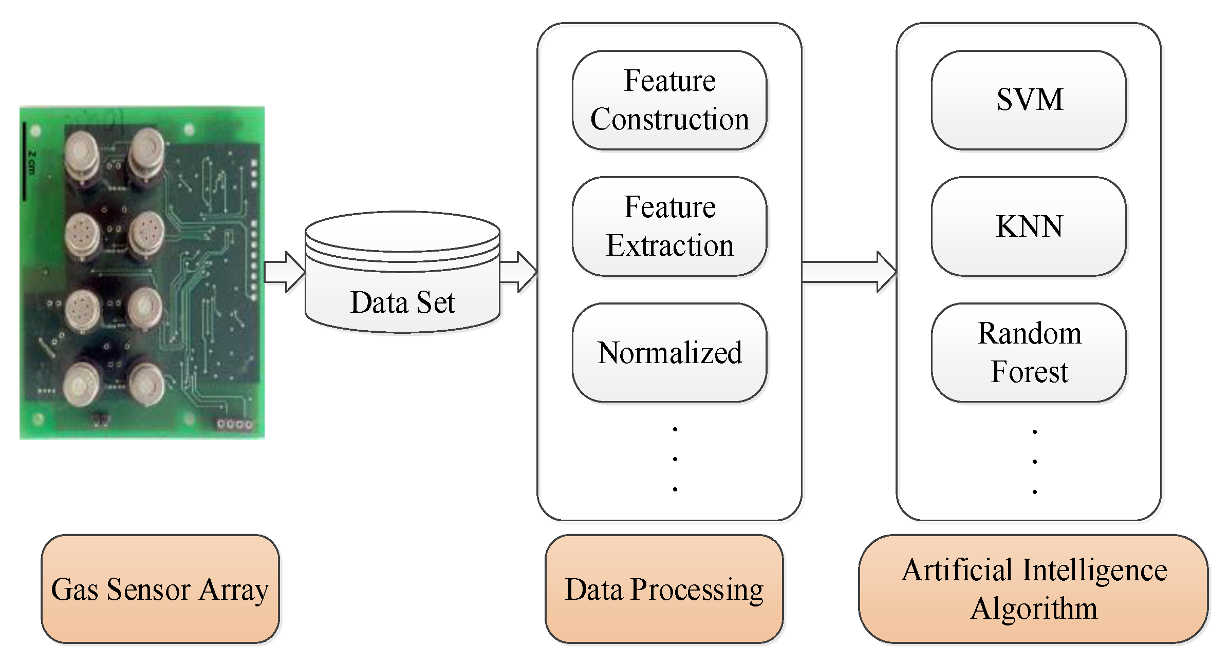
The main aspects of machine olfaction include the gas sensor array, data processing and artificial intelligence algorithms as shown in the overall schematic diagram shown in Figure 1 [10]. The overall operational process of the system is to first obtain the gas information through the sensor array; the multi-dimensional data represented by the array can fully characterize the gas type information. After the data are stored and classified, feature extraction and selection are carried out through data analysis and feature engineering, and the processed data of the feature engineering is used by an algorithm to identify the gas. Among them, the artificial intelligence algorithms have an extremely important role, and their accuracy, time efficiency and anti-interference ability all affect the decision-making result of the whole system [11,12,13]. In [14], researchers consider that only by adopting the optimal data processing algorithm can the performance of the whole model for machine olfaction be improved. Studies [15] proposed that reasonable improvement of the algorithm is an important support for the development of the current machine olfaction systems.
Based on an experimentally acquired metal oxide semiconductor (MOS) gas sensor array dataset, researchers focus on a machine learning classification algorithm to improve the detection accuracy of mixed gas [16,17,18]. In the current field of mixed gas detection, many researchers have applied algorithms to achieve good classification results, such as support vector machine (SVM), artificial neural network (ANN), K-nearest neighbour (KNN), etc. [19,20,21,22,23,24,25]. To improve the classification accuracy, Sun proposed an optimized AdaBoost algorithm [26]. The M2 model combined multiple classifiers and performed multiple classification experiments using different fusion rules. The final highest recognition accuracy obtained was 91.75%. In [27], the posterior probability estimation algorithm extracted from an SVM was used to detect 10 kinds of bacterial components in the human blood by machine olfaction, and the recognition accuracy was high, but the time cost was large. In [28], the probabilistic Bayesian algorithm was used to solve the uncertainty relationships in gas source localization, and the Markov decision process path planning algorithm was used to improve the gas localization efficiency. In [29], the artificial neural network (ANN) algorithms improved the resolution of the moisture content detection in soil, but the ANN algorithm lacks explanation. At present, few researchers can improve the time efficiency of the algorithm under the condition of high detection accuracy [30]. Moreover, few researchers consider the accuracy of the gas sensor itself. While the traditional feature extraction method, the principal component analysis (PCA), is a dimensionality reduction operation, when the algorithm’s dimensionality is not high enough, it is necessary to construct its features. In addition, among the classification algorithms, there are few algorithms that have strong anti-overfitting ability as well as a high training speed, training time efficiency, and classification accuracy [31,32].
To improve the anti-overfitting ability and accuracy for machine olfactory detection of mixed gases, this paper proposes a data screening method based on a dynamic time warping algorithm (DTW) to improve the gas classification accuracy. To address the problem of too few features, the PCA feature construction and extraction methods are proposed. The proposed new extreme random tree algorithm is used to further improve the detection and analysis performance of the machine olfactory system [33,34].
Taking carbon monoxide, methane and ethylene as examples, this paper studies a mixed gas detection algorithm based on extreme random trees to improve the classification accuracy rate. It can provide mixed gas detection and concentration ratio technical support for industrial production, chemical material production, and the light industry [35,36,37]. This study provides a theoretical reference for the simulation of olfactory algorithms.
The main points raised in this paper are as follows:
(1) To improve the classification accuracy and time efficiency of mixed gas detection, the random forest algorithm is improved. This paper proposes a new classification algorithm called DTW-Extra tree. The similarity processing of the data is mainly carried out by the DTW algorithm so that the discrimination among the data is improved. Feature extraction is carried out by a feature construction method. Finally, the extra-tree algorithm is used for gas classification to improve the classification accuracy and time efficiency.
(2) The mixed gas datasets of ethylene and carbon monoxide; and ethylene and methane were obtained experimentally, and the proposed algorithm was verified experimentally. The analysis shows that the algorithm has higher accuracy for gas classification and improves the time efficiency of the random forest algorithm.
The content of this paper is organised as follows: Section 2 introduces the gas detection algorithm research, including the dynamic time warping algorithm (DTW), feature construction, feature extraction, principal component analysis and the extreme random tree algorithm. Section 3 carries out experimental verification and analyses the results. Section 4 summarizes the conclusions and results.
2. Hybrid Gas Detection Method
2.1. Dynamic Time Warping Algorithm
An effective data pre-processing method can greatly improve the accuracy of the algorithm. Since the mixed gas data are based on a time series of gas signal response curves, dynamic time warping is performed on the dataset. Dynamic time warping is an algorithm that is based on dynamic programming (DP) [38]. It optimizes the misalignment of the feature parameters. Its basic principle is to find the optimal curved path between the time series. The coordinates of the data points in a sequence are used to find the points with the most identical features, and the sum of the distances between the data points is the sum of the optimal curved paths [39,40].
Suppose the two time series are where the length of the two time series is m and n, respectively. is a distance matrix constructed from the two time series:
where in is obtained by calculating the coordinate distance between and ; its calculation process is:
When w = 2, it is equal to the Euclidean distance 2-norm. The curved path, with the smallest distance through is equivalent to the DTW distance between the two time series.
is the current cumulative distance of the curved path when searching .
The three conditions for the search for p are as follows: (1) a fixed starting point, the starting point of the path is , and the ending point is . (2) monotonic consistency, set the current point, of the search, the current cumulative distance is , and, , . (3) consistent continuity, let the current point of the search be , the current cumulative distance is , , and , . The above three conditions are set and the starting position of the search path is determined by the first point; the second three points determine that the position of the next point of the search path is on the right side, the upper side or the upper right side of the current point, if the current point is , and assuming that the search point is at this time, the calculation is:
Finally, is obtained, and the cumulative distance averaging process is used to solve the case where the sequence length and the cumulative distance are different:
d is the average cumulative distance from the two sequences [41,42,43].
Due to the limitation of the three-point constraint, the DTW algorithm traverses all the observation points, and each original sequence can find the corresponding point. By calculating the average cumulative distance, the sample is initially screened from the original data.
2.2. Feature Construction Method
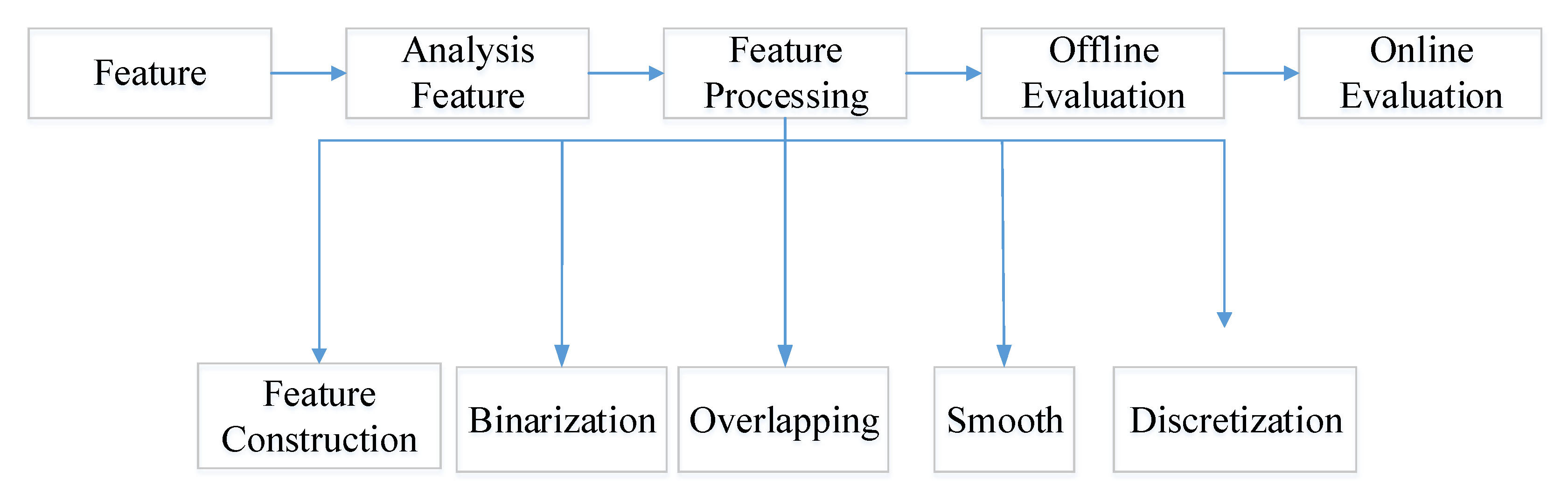
The original dataset has 8-dimensional features. To improve the classification accuracy, the data features are constructed, and the characteristics of the different features are compared to find the best features for classification. The reason for feature construction is that the training data determines the highest accuracy that can be achieved. Appropriate feature construction can increase the useful information in the data, which helps to improve the classification accuracy of the model [44,45,46]. Therefore, based on the original features, the accuracy of the classification algorithm is improved by constructing new features. The specific feature engineering method is shown in Figure 2 below:
The commonly used feature construction methods have interactive features, such as features A and B, that create features A × B, A − B, A/B and A + B, which will cause the feature space to explode [47,48,49]. If there are 10 features and if two variable interaction features are created, this will be 90 features in the model.
The features applied in this research are 8-dimensional features. The created features are A − B and A/B. After the interactive features are created, the number of features is 56, which provides the multidimensional features for subsequent feature extraction.
2.3. Principal Component Analysis
The principal component analysis (PCA) method is a commonly used statistical method [50]. By calculating the original data covariance matrix, the high-dimensional data are transformed into low-dimensional data and the correlation between the dimensions is determined. The purpose of principal component analysis is to reduce noise and redundancy. The noise reduction is to ensure that the correlation between the processed data is as small as possible. The redundancy is removed to maximize the variance of the processed data [51,52].
Suppose that there are p sensors, n samples are collected and a matrix X is formed. The number of rows of X is n, and the dimension is p, which can be expressed in the form of a column vector, as shown in Equation (7):
Convert the p-dimensional data into linear combinations of p variables:
where are the values after the linear transformation and the equation satisfies the following conditions: (1) are irrelevant to each other. (2) The magnitude relationship of the variance is (3) . Therefore, represents the principal components of the initial variables, , and is called the principal component coefficient.
The specific implementation steps of the principal component analysis are as follows:
(1) Standardize the raw data
The PCA is a data-based covariance matrix. The size of the data varies. To keep the dimensions of the data consistent, the data should be standardized first. Subtract the data from the mean of the dimension and divide by the standard deviation of the dimension.
represents the mean of the data, and represents the variance of the data.
(2) Calculate the covariance matrix of the data
The covariance matrix of the normalized data is the correlation coefficient matrix of the original variables. The derivation is as shown in Equation (10).
The correlation coefficient matrix R can be expressed as:
From the feature equation, , solving for the eigenvalue of the correlation coefficient matrix yields , and the eigenvectors are ordered by the eigenvalues from large to small, . Substitute into . Solve for the feature vector, , and unitize into .
(4) Find the principal component by calculating the cumulative contribution rate.
Calculate the cumulative contribution rate of the aligned eigenvalues. Generally, when the top t features are worth accumulating, they have a cumulative contribution rate of 85%–95%; one can take these t features as the main components:
(5) Find the load of the principal component.
The principal component, , is obtained from Equation (8).
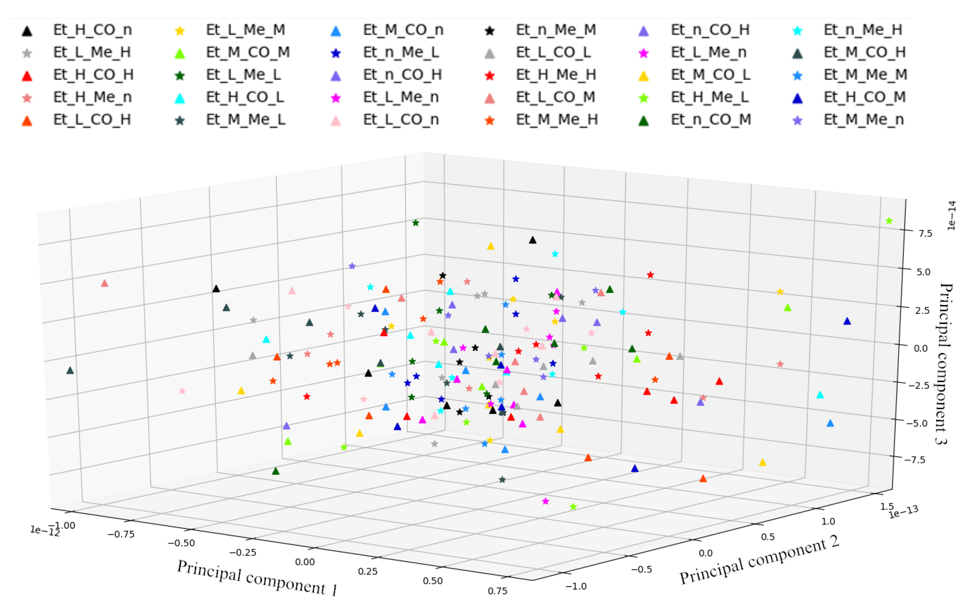
To illustrate the discreteness of the data features, I abstracted all the data and each category into three-dimensional features. As shown in Figure 3, the features have obvious discrete types, and the traditional single dimension algorithm cannot complete the classification. The classification results in the untreated case are analysed in the Analysis Verification section.
2.4. Extreme Random Tree Algorithm
2.4.1. Random Forest Algorithm
Random forest is an integrated algorithm that uses bagging and random subspace to generate decision trees. It combines multiple decision trees through voting rules. When the data are input, the classifier passes the data to each decision tree. Each tree in the forest will have a classification result, and, finally, multiple decision trees vote to produce the final result [53].
Suppose D is a dataset with M-dimensional features [54,55]. The specific implementation method for the random forest algorithm is as follows:
(1) The training subset, is generated from the original dataset, D (i.e., bootstrap sampling), and the remaining data become the corresponding training subset, .
(2) The CART algorithm is adopted for the dataset to construct the decision tree. At each node for splitting the decision tree, random samples are taken from all the features to generate an m-dimension feature subspace . All the possible splitting nodes are calculated against the features, and the optimal splitting node is selected for splitting. The decision tree is split until the decision tree’s pre-set stop depth is reached. Each of the trees is grown without pruning, and K decision trees are generated.
(3) Integrate into a random forest and use the voting results of all the trees as the classification decision of the random forest. Therefore, after the data are classified, the results of all the trees passing the vote is the classification result of the random forest output [56].
2.4.2. Extreme Random Tree Algorithm
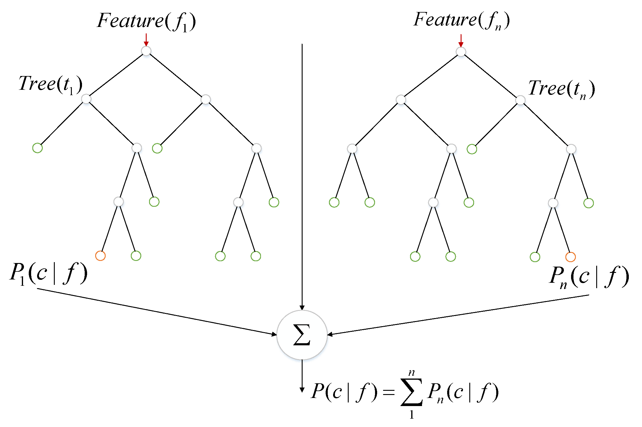
The Extreme Random Tree is similar to the random forest algorithm [57]; it is integrated by multiple decision trees and thus has many of the same advantages. For example, it has an excellent classification effect and high accuracy, and high-dimensional feature data can be processed effectively without using feature selection. The execution process can be parallelized for efficiency. For mixed gas detection and classification, the integrated learning algorithm has higher classification accuracy, but each decision tree uses all the original data in the extreme random tree algorithm, while the random forest algorithm uses bootstrap sampling to generate the training samples. When the extreme random tree splits at a node, the splitting node is randomly selected, and the optimal splitting threshold or feature is not selected. Figure 4 is a schematic diagram of an extreme random tree algorithm.
The following is an analysis of the difference between the extreme random tree and the random forest algorithm:
First, the training samples of the random forest algorithm are generated by bootstrap sampling. However, each decision tree in the extreme random tree uses all the original training sample data, which helps to reduce the variation of the model.
Second, when the node is split, the random forest classification algorithm first selects some features from all features, and then accurately selects the best split mode (such as the Gini index) through splitting according to these features to generate the decision tree. The extreme random tree algorithm is a random splitting selection method. The specific implementation process is as follows: for splitting the category form, randomly select some categories of data to put into one branch and put the other categories of data into another branch; for numerical form splitting, a threshold between the maximum and minimum value is randomly selected, which is the data principle of the left and right branches. Data larger than the threshold value are put into one branch, while data smaller than the threshold value are put into another branch. Then, for the classification problem in this paper, the GINI index is used to calculate the split value. Traverse all the features of the node and obtain all the feature split values, and select the feature with the largest split value for splitting (for the regression problem, use the mean square error to calculate the split value).
In the extreme random tree algorithm, since all the training data samples are OOB (out of bag) data samples, the calculation of the prediction error for the extreme random tree is the error calculation for the OOB sample. In the research of this subject, it is found that the extreme random tree is superior to the random forest algorithm in terms of the time efficiency of training, accuracy of classification, and ability to fit training data [58].
The specific implementation steps of the extreme random tree are as follows:
The extreme random tree algorithm is represented by , where denotes a classifier model, denotes a raw data sample, and denotes the number of decision trees. Each decision tree produces a prediction result based on the sample input and finally obtains a classification decision according to the voting rule.
(1) In the classification model of the extreme random tree, each base classifier uses all the training samples (OOB samples) for training, assuming the original dataset, , the number of samples, , and the number of features, .
(2) Generate a decision tree according to the classification and regression tree (CART) algorithm. In the process of node splitting, M features are randomly selected from the M features in each splitting node, some categories are randomly selected and put into one branch, and the remaining categories are put into another branch. Meanwhile, the optimal splitting value of each node is calculated, and the optimal attribute splitting is selected; no pruning operation is performed in the splitting process. Iteratively split the subsets to a present value to generate a decision tree.
(3) Repeat steps (1) and (2) for K times, and finally, an extreme random tree model composed of K decision trees is generated.
(4) Test the extreme random tree model, trained through test data, and finally generate the final classification result through voting.
The advantages of the extreme random tree (ET) algorithm are as follows: (1) ET is an integrated learning algorithm, which generates the predicted results through voting decisions and has a strong generalization ability; (2) ET uses all the data (OOB samples) to train the base classifier, so that all samples are trained; and (3) due to the random selection in node splitting, the randomness is greatly enhanced.
3. Analysis of Experiment Results and Discussion
To verify the effectiveness of the proposed classifier, a 10-fold cross-validation method was used to analyse and verify the original ethylene and methane sample and the ethylene and carbon monoxide sample. The specific classification results and analyses are as follows.
3.1. Data Analysis
For the 180 datasets collected by the machine olfactory data acquisition system, ethylene-methane and ethylene-carbon monoxide were mixed together. Each tag consists of six experiments to form a different dataset. The duration of the data sampling phase is 300 s, and there is no air inlet in the first 60 s. At 60 s, the mixed gas with a set concentration ratio is injected into the air chamber. The entire inlet time of the mixed gas is 180 s, and, during the last 60 s, there is no inlet for the mixed gas. The sensor array consists of eight sensors with sensor frequency set at 50 Hz and a mixed gas dataset acquired from eight sensors. Each dataset contains time (s), temperature, humidity (%) and the sensor resistance values of TGS2600, TGS2612, TGS2611, TGS2610, TGS2602, TGS2602, TGS2620, and TGS2620. The data collected by the sensor is the voltage value of the external load resistor , and the sensor resistance is represented by , where the relationship between and is:
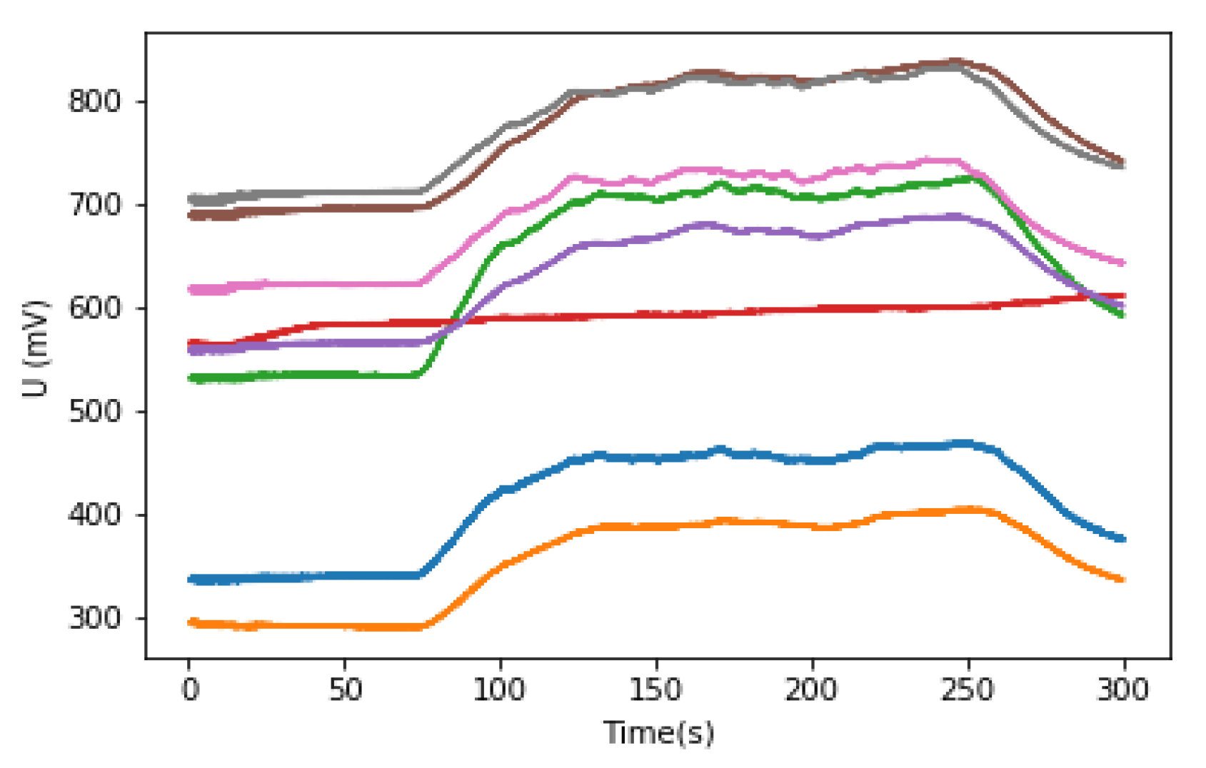
In the air, the resistance value of is large, and the voltage value of is small. After the gas is injected, the sensors respond, decreases, and the voltage value of becomes larger. Therefore, the mixed gas category can be detected by the datasets of the voltage value . The collected datasets have a total of 30 categories, as shown in Table 1. The sensor response plot for an experiment is shown in Figure 5 (in the case of Et_H_Me_n), the abscissa is time and the ordinate is the converted sensor voltage value.
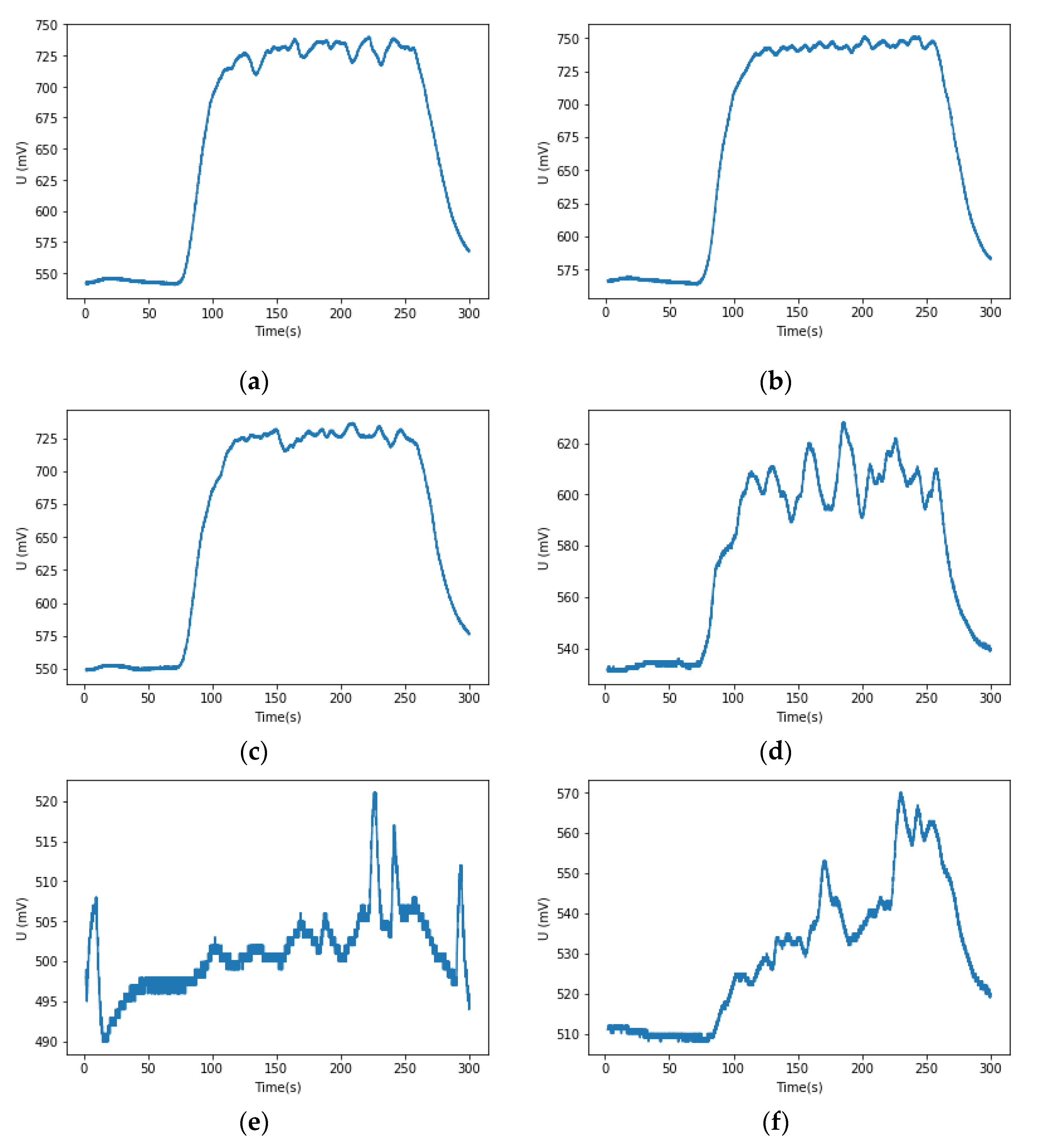
To investigate the data collected by the sensor, a response curve analysis is performed for the TGS2602 under the same label (i.e., the Et_M_Me_M label), such as Figure 6. It can be seen that the same sensor has different degrees of response in the same situation and the Figure 6e sensor response curve was found to be significantly different from the Figure 6a. Therefore, it can be inferred that, in the experiments, due to problems such as the configuration of the experimental conditions, different degrees of data inconsistency under the same label may occur. An accurate single mixed gas classification result cannot be obtained from only a single output of the sensor, and data pre-processing should be performed to improve the classification effect.
3.2. Verification of the DTW Algorithm
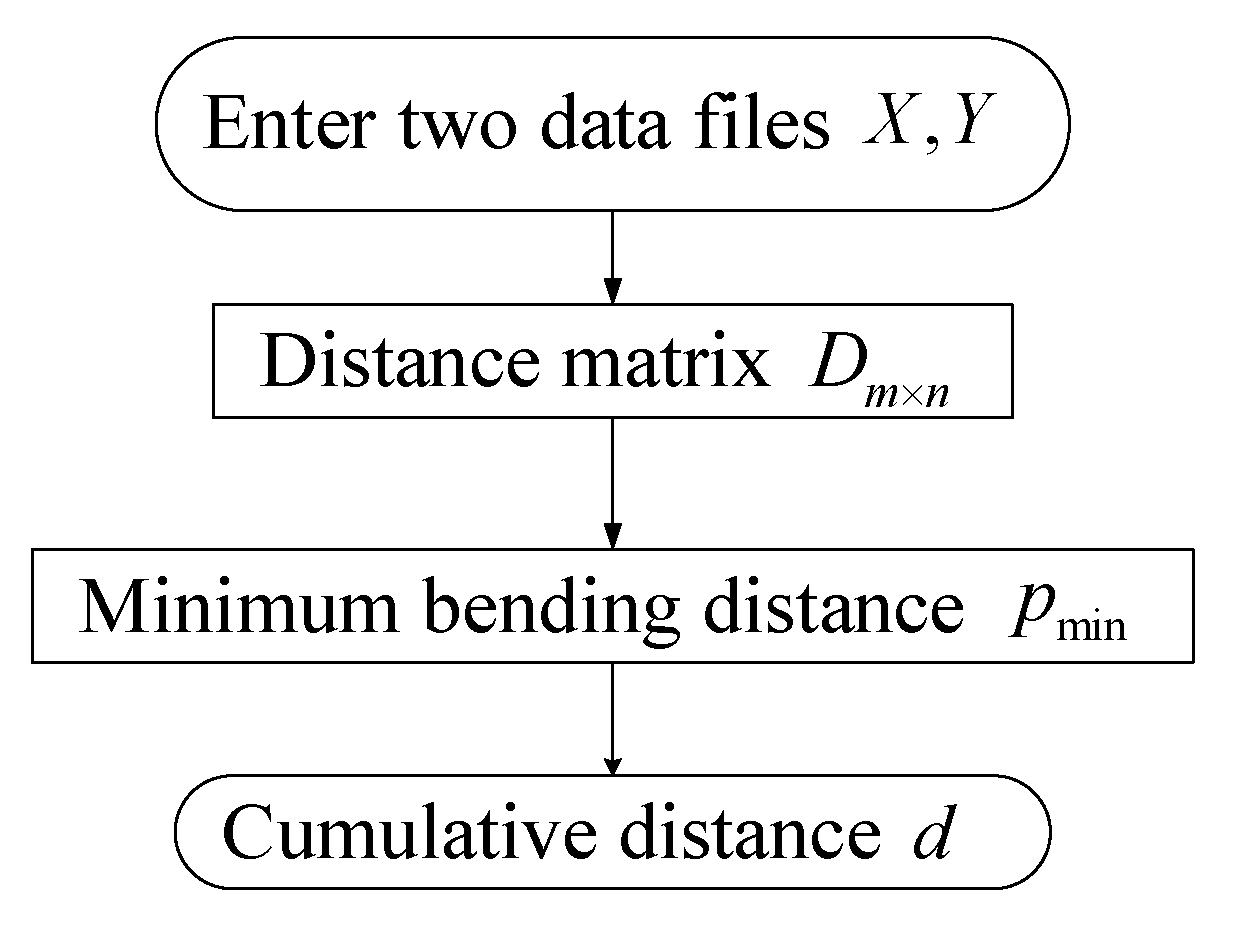
Due to the analysis of the datasets, it is difficult to meet the classification accuracy requirement by using the datasets directly. In this paper, the DTW algorithm is adopted to filter the similarity of data, and the specific operation steps are shown in Figure 7. This algorithm will match all the cases in the mixed gas datasets, and then calculate the average cumulative distance between the two groups according to the six sets of data in each category. The preliminary screening datasets are sorted according to the size of the d value. This type of operation is performed on all category data to obtain a processed dataset.
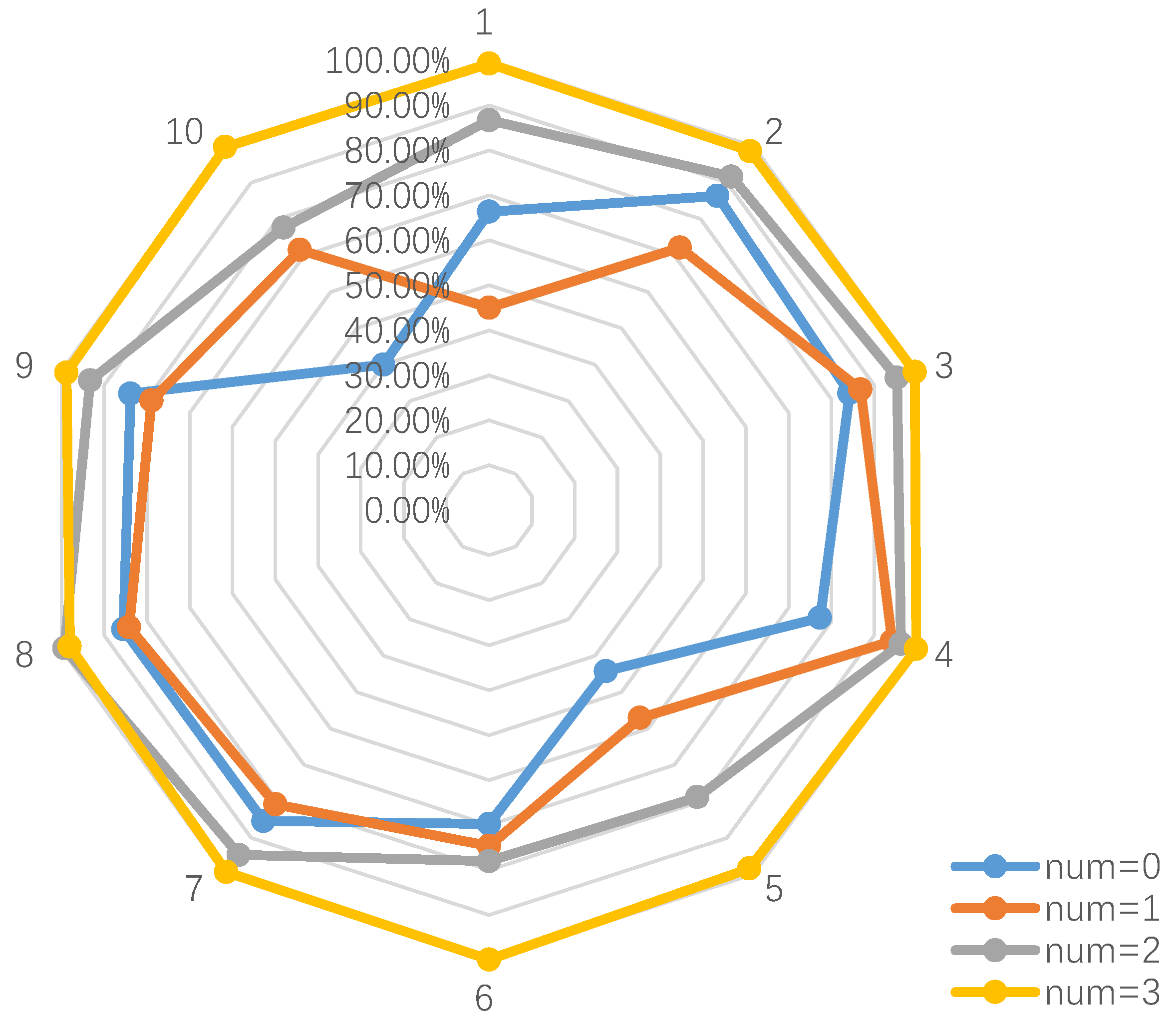
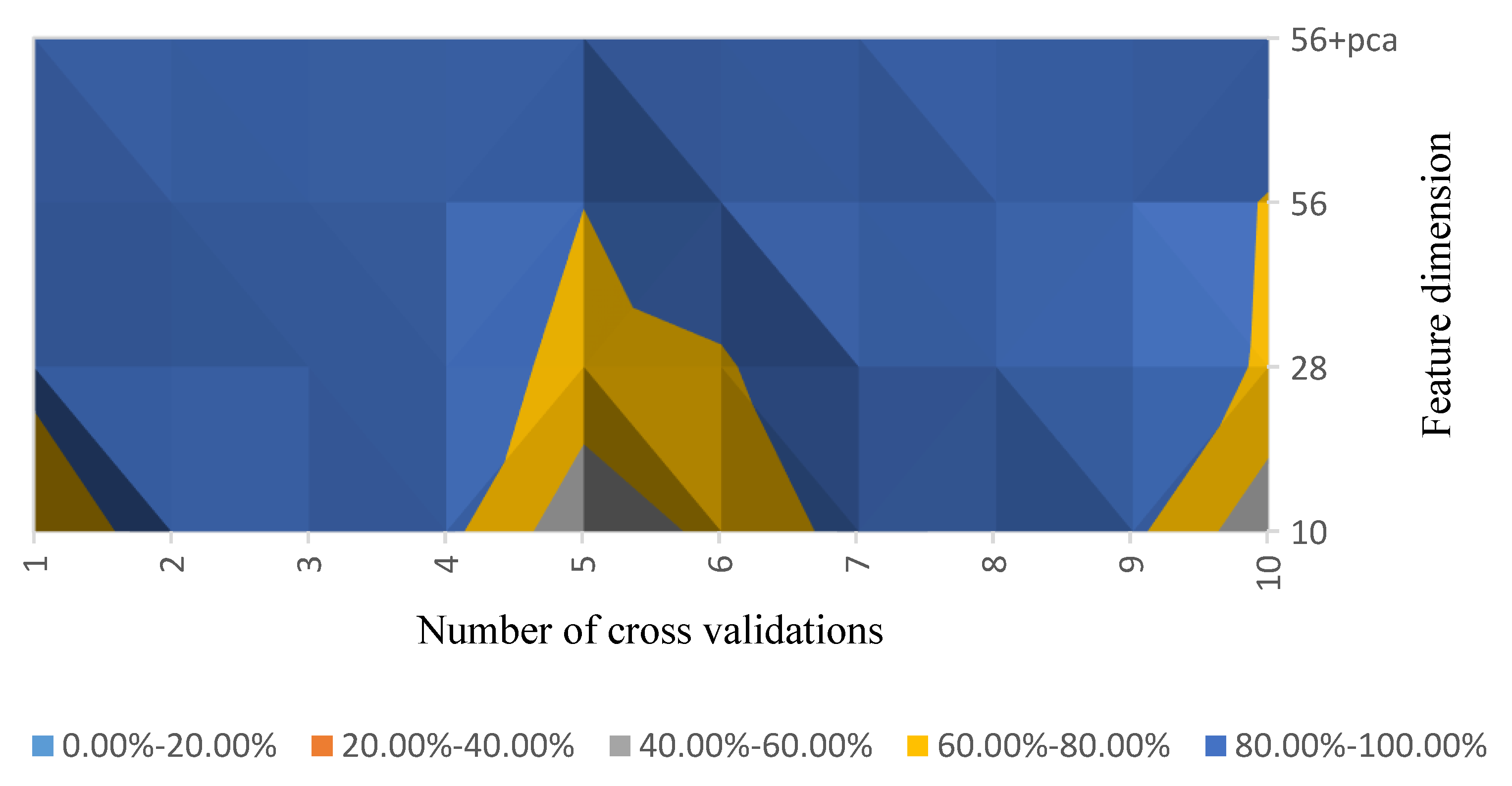
In the dynamic time warping (DTW) algorithm, we set the benchmark parameter, num, to 1, 2 and 3 and tested without using the DTW. The results are shown in Figure 8.
As can be seen from Figure 8, the more the area enclosed by the fold line, the higher the classification accuracy. The num = 3 yellow fold line encloses the largest area, and the num = 2 gray fold line envelops the area at the middle position, while the num = 0 blue and num = 1 orange fold lines surround the area, which are all smaller. Combined with the data in Table 2, it can be seen that when num = 3, the 10-fold cross-validation accuracy rate is 99.17%. Compared with num = 2, num = 1 and num = 0, the accuracy is improved by 10.00%, 24.64% and 26.87%, respectively. Therefore, it can be concluded that after DTW, the effect of the model is significantly improved, and the accuracy of classification is greatly improved.
3.3. Feature Construction and PCA Algorithm Validation
We use feature construction to increase the data dimension and select the best features for training. The results are shown in Figure 9.
The analysis shows that, if the feature dimension is kept unchanged, the recognition accuracy is only 73.37%, and if the dimension is increased by A-B, it becomes a 28-dimensional data feature, and the recognition accuracy increases to 87.50%. It can be seen that a purposeful elevated dimension has a good effect on the classification accuracy. Therefore, after the feature is upgraded to 56-dimensions, the recognition rate is 18.97% higher than that of the original dimension, and the final recognition rate is 99.17% after the response is reduced by the PCA algorithm.
3.4. Extreme Random Tree Verification Analysis
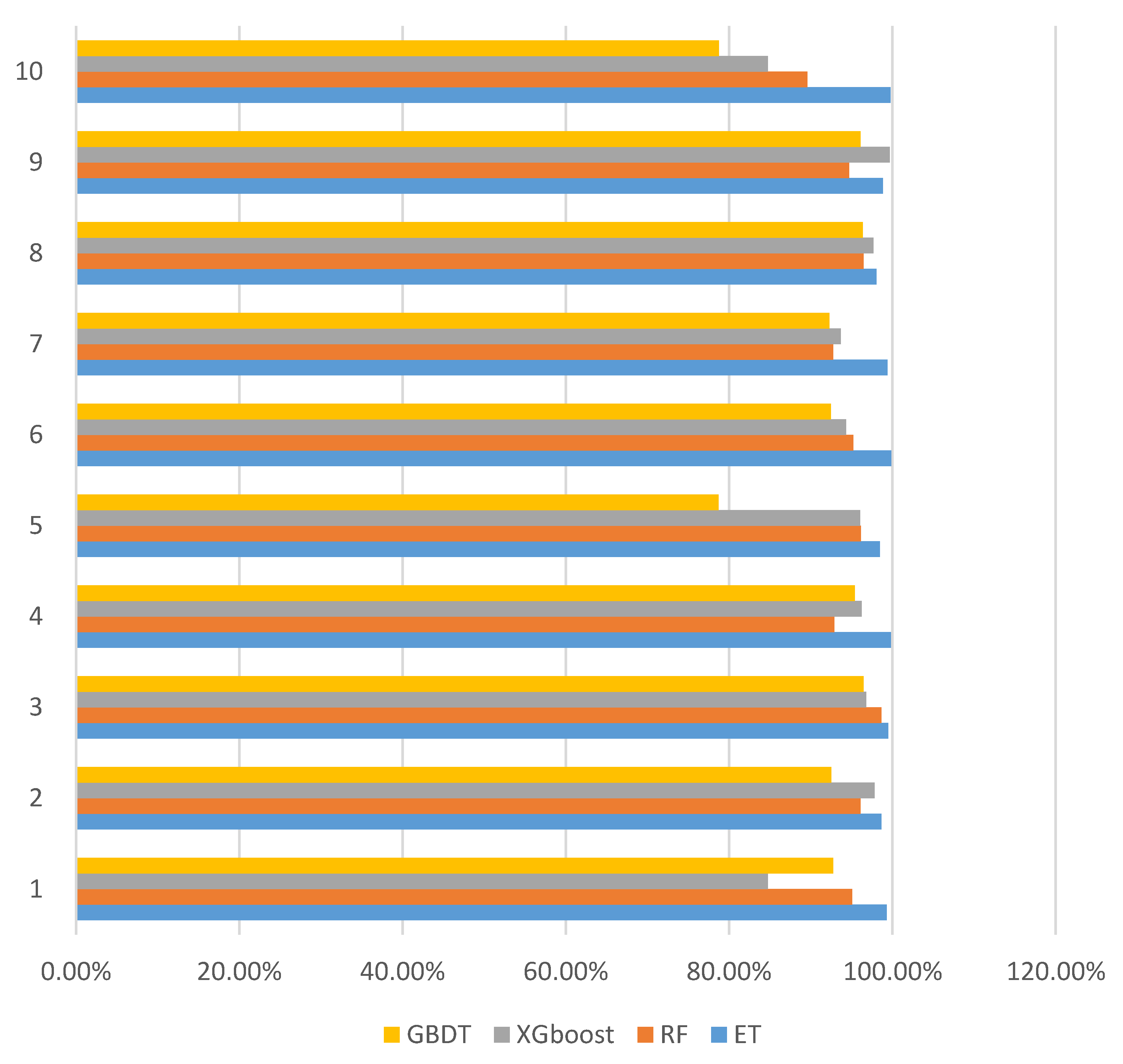
After many algorithms are compared, among the current integrated learning classification algorithms, the random forest algorithm is the most common most effective. Therefore, a comparative experiment is carried out with the extreme random forest algorithm. The accuracy and time efficiency of the XGBoost and GBDT algorithms are also compared. Figure 10 and Table 3 show that the extreme random tree algorithm is 4.42% more accurate than the random forest algorithm, 5.00% more accurate than the XGboost algorithm, and 7.99% more accurate than the GBDT algorithm.
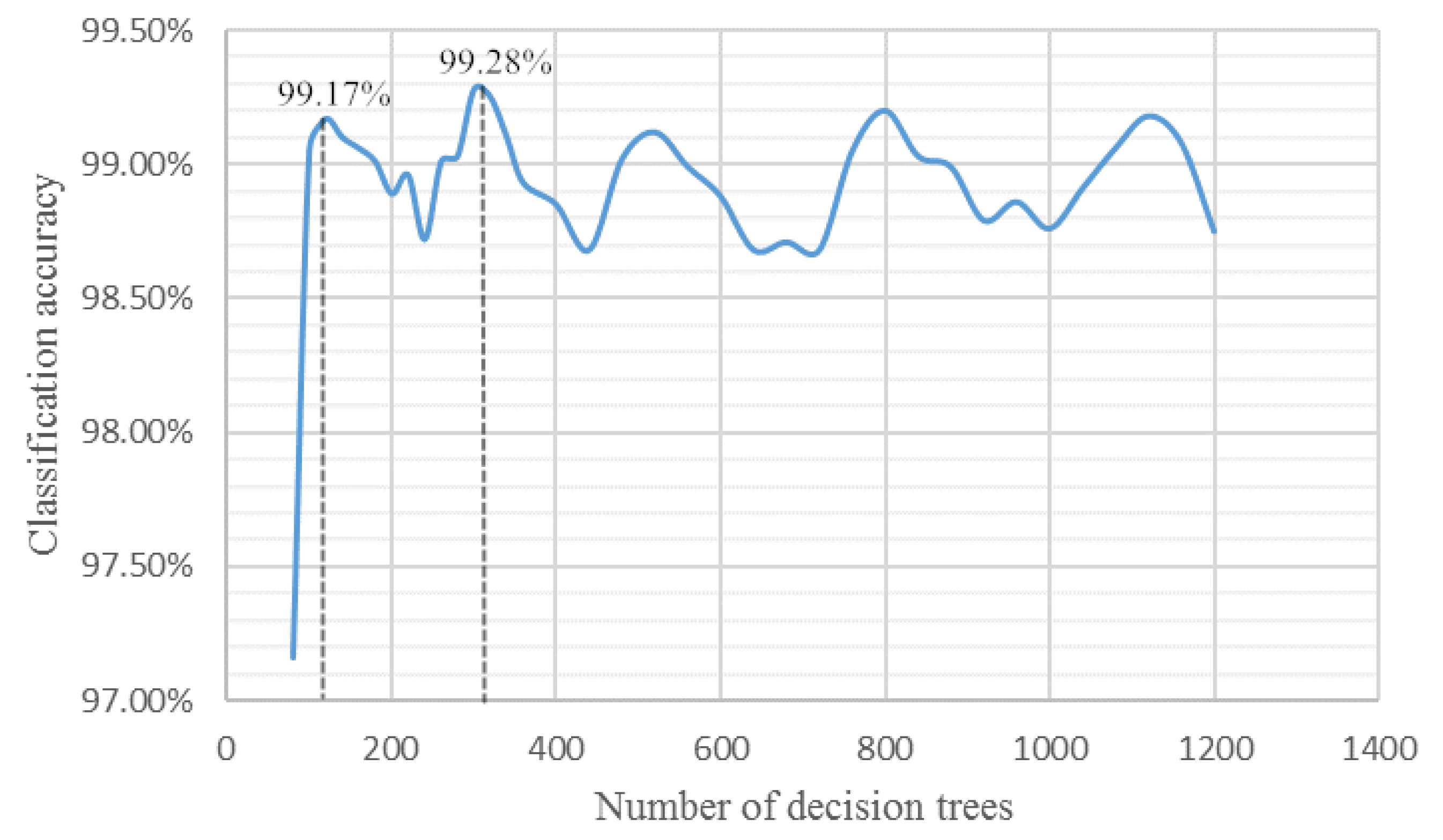
In the above model construction, the number of decision trees in the extreme random tree was 120. However, the number of decisions trees affected the accuracy of the model. The experimental results for the number of decision trees are shown in Figure 11. There are several important data points, which are peaks in the image when the number of decision trees is 120, 300, 500, 800, and 1100. Because of a small number of decision trees, it is easy to cause the underfitting state. If the number of decision trees is too large, the improvement of algorithm accuracy is not of great significance. When the number of decision trees is 300, the classification accuracy reaches the highest 99.28%.
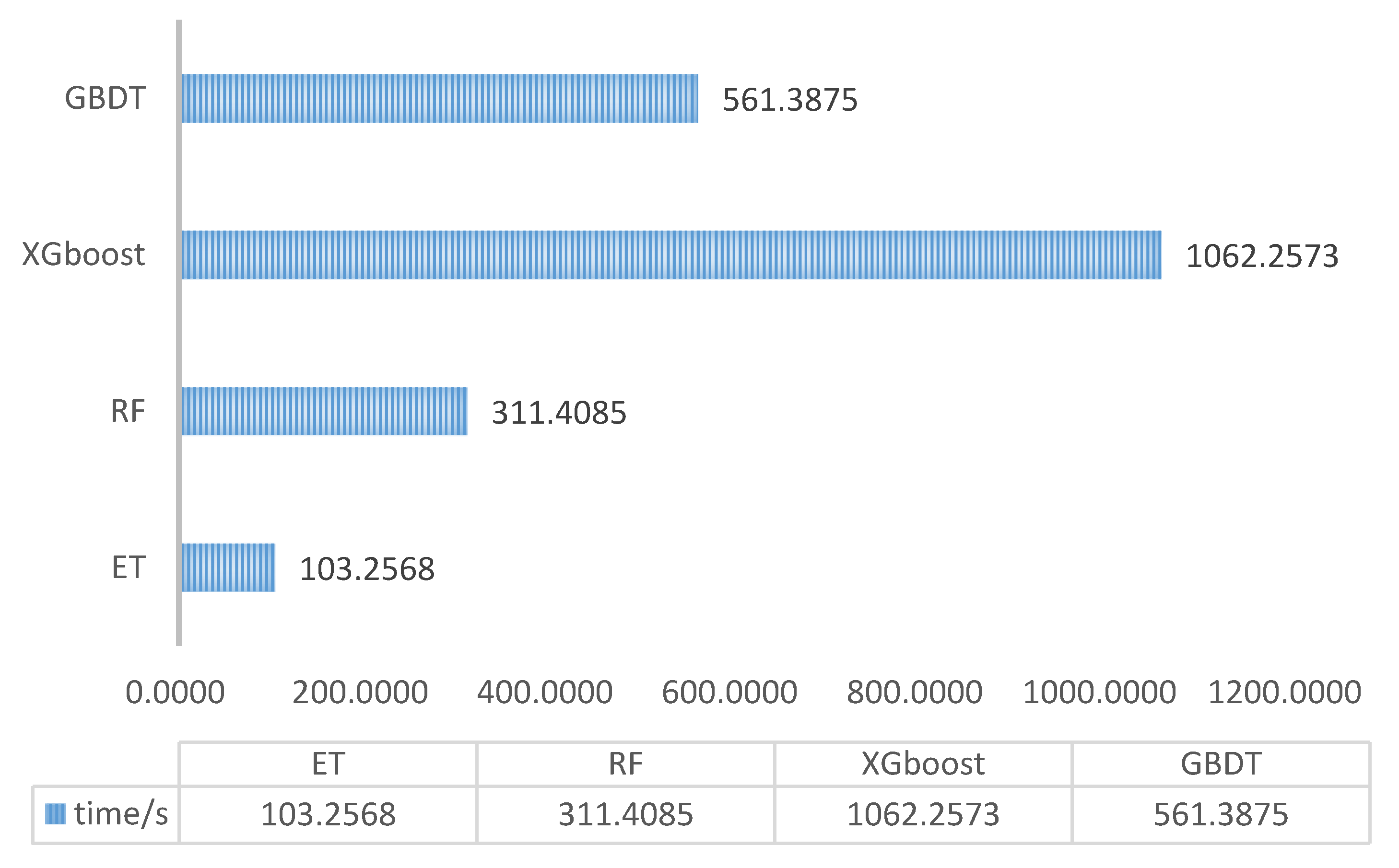
The results from the experiments for the runtime of the algorithms are shown in Figure 12. The extreme random tree algorithm has the shortest running time of only 103.2568 s, which is 66.85% lower than that of the random forest algorithm. The XGBoost algorithm has the longest running time because it is the most complex model.
Therefore, the proposed extreme random tree algorithm achieves a significant improvement in accuracy and time efficiency.
4. Conclusions
Considering the low detection accuracy of current machine olfactory systems, this paper proposes a dynamic time warping algorithm based on DTW, which improves the classification accuracy by 26.87%. Based on original feature construction and the PCA method, the classification accuracy rate increased by 25.8%. Finally, the time efficiency problem in the random forest algorithm is improved by the extreme random tree algorithm. The final classification accuracy rate is 99.28%, and the run time of only 103.2568 s is 66.85% lower than that of the random forest algorithm. Through the method proposed in this paper, the classification problem of mixed gases is solved, and the random forest algorithm is improved to a large extent, which improves the classification accuracy of the machine olfactory system and provides a theoretical basis for an algorithm to simulate the olfactory nervous system.
Author Contributions
Y.X., X.Z., Y.C. and Z.Y. conceived and designed the experiment. Y.X. was responsible for the research direction and guidance of algorithm innovation of the whole paper, and proposed the improved extreme random tree algorithm. X.Z. did some simulation experiments of the algorithm and wrote the paper. Y.C. reviewed and edited the manuscript. Z.Y. performed signal preprocessing and implemented the DTW algorithm.
Funding
This work is financially supported by the Natural Science Foundation of China (Grant No. 61803128).
Conflicts of Interest
The authors declare no conflict of interest.
References
- Climent, E.; Pelegri-Sebastia, J.; Sogorb, T.; Talens, J.B.; Chilo, J. Development of the MOOSY4 eNose IoT for Sulphur-Based VOC Water Pollution Detection. Sensors 2017, 17, 1917. [Google Scholar] [CrossRef]
- Xu, Y.; Zhao, X.; Chen, Y.; Zhao, W. Research on a Mixed Gas Recognition andConcentration Detection Algorithm Based on a MetalOxide Semiconductor Olfactory System Sensor Array. Sensors 2018, 18, 3264. [Google Scholar] [CrossRef] [PubMed]
- Murthy, V.N.; Dan, R. Processing of Odor Mixtures in the Mammalian Olfactory System. J. Indian I Sci. 2017, 97, 415–421. [Google Scholar] [CrossRef]
- Li, W.; Liu, H.; Xie, D.; He, Z.; Pi, X. Lung Cancer Screening Based on Type-different Sensor Arrays. Sci. Rep. 2017, 7, 1969. [Google Scholar] [CrossRef]
- Haridas, D.; Chowdhuri, A.; Sreenivas, K.; Gupta, V. Fabrication of SnO2 Thin Film Based Electronic Nose for Industrial Environment. In Proceedings of the IEEE Sensors Applications Symposium, Limerick, Ireland, 23–25 February 2010; Volume 143, pp. 173–189. [Google Scholar]
- Yan, K.; Zhang, D. Calibration transfer and drift compensation of e-noses via coupled task learning. Sens. Actuators B Chem. 2016, 225, 288–297. [Google Scholar] [CrossRef]
- Yan, K.; Zhang, D. Improving the transfer ability of prediction models for electronic noses. Sens. Actuators B Chem. 2015, 220, 115–124. [Google Scholar] [CrossRef]
- Laref, R.; Losson, E.; Sava, A.; Adjallah, K.; Siadat, M. A comparison between SVM and PLS for E-nose based gas concentration monitoring. In Proceedings of the 2018 IEEE International Conference on Industrial Technology (ICIT), Lyon, France, 20–22 February 2018. [Google Scholar]
- Fu, G.; Zhao, Z.Q.; Hao, C.B.; Wu, Q. The Accident Path of Coal Mine Gas Explosion Based on 24Model: A Case Study of the Ruizhiyuan Gas Explosion Accident. Processes 2019, 7, 73. [Google Scholar] [CrossRef]
- Green, G.C.; Chan, A.D.C.; Dan, H.H.; Lin, M. Using a metal oxide sensor (MOS)-based electronic nose for discrimination of bacteria based on individual colonies in suspension. Sens. Actuators B Chem. 2011, 152, 21–28. [Google Scholar] [CrossRef]
- Giungato, P.; Laiola, E.; Nicolardi, V. Evaluation of industrial roasting degree of coffee beans by using an electronic nose and a stepwise backward selection of predictors. Food Anal. Methods 2017, 10, 3424–3433. [Google Scholar] [CrossRef]
- Romain, A.C.; Nicolas, J. Long term stability of metal oxide-based gas sensors for e-nose environmental applications: An overview. Sens. Actuators B Chem. 2010, 146, 502–506. [Google Scholar] [CrossRef] [Green Version]
- Neumann, P.P.; Hernandez Bennetts, V.; Lilienthal, A.J.; Bartholmai, M.; Schiller, J.H. Gas source localization with a micro-drone using bio-inspired and particle filter-based algorithms. Adv. Robot. 2013, 27, 725–738. [Google Scholar] [CrossRef]
- Craven, M.A.; Gardner, J.W.; Bartlett, P.N. Electronic noses—Development and future prospects. TrAC Trends Anal. Chem. 1996, 15, 486–493. [Google Scholar] [CrossRef]
- De Cesare, F.; Pantalei, S.; Zampetti, E.; Macagnano, A. Electronic nose and SPME techniques to monitor phenanthrene biodegradation in soil. Sens. Actuators B Chem. 2008, 131, 63–70. [Google Scholar] [CrossRef] [Green Version]
- Smolarz, A.; Wojcik, W.; Gromaszek, K. Fuzzy modeling for optical sensor for diagnostics of pulverized coal burner. Procedia Eng. 2012, 47, 1029–1032. [Google Scholar] [CrossRef]
- Ray, M.; Ray, A.; Dash, S.; Mishra, A.; Achary, K.G.; Nayak, S.; Singh, S. Fungal disease detection in plants: Traditional assays, novel diagnostic techniques and biosensors. Biosens. Bioelectron. 2017, 87, 708–723. [Google Scholar] [CrossRef]
- Cellini, A.; Biondi, E.; Blasioli, S.; Rocchi, L.; Farneti, B.; Braschi, I.; Savioli, S.; Rodriguez-Estrada, M.T.; Biasioli, F.; Spinelli, F. Early detection of bacterial diseases in apple plants by analysis of volatile organic compounds profiles and use of electronic nose. Ann. Appl. Biol. 2016, 168, 409–420. [Google Scholar] [CrossRef]
- Fang, Y.; Umasankar, Y.; Ramasamy, R.P. A novel bi-enzyme electrochemical biosensor for selective and sensitive determination of methyl salicylate. Biosens. Bioelectron. 2016, 81, 39–45. [Google Scholar] [CrossRef] [Green Version]
- Xu, S.; Lv, E.; Lu, H.; Zhou, Z.; Wang, Y.; Yang, J.; Wang, Y. Quality Detection of Litchi Stored in Different Environments Using an Electronic Nose. Sensors 2016, 16, 852. [Google Scholar] [CrossRef]
- Meksiarun, P.; Ishigaki, M.; Huck-Pezzei, V.A. Comparison of Multivariate Analysis Methods for Extracting the Paraffin Component from the Paraffin-Embedded Cancer Tissue Spectra for Raman Imaging. Sci. Rep. 2017, 7, 44890. [Google Scholar] [CrossRef]
- Messina, V.; Domínguez, P.G.; Sancho, A.M.; Walsöe de Reca, N.; Carrari, F.; Grigioni, G. Tomato Quality during Short-Term Storage Assessed by Colour and Electronic Nose. Int. J. Electrochem. 2012, 2012, 1–7. [Google Scholar] [CrossRef] [Green Version]
- Baietto, M.; Wilson, A.D.; Bassi, D.; Ferrini, F. Evaluation of Three Electronic Noses for Detecting Incipient Wood Decay. Sensors 2010, 10, 1062–1092. [Google Scholar] [CrossRef] [Green Version]
- Dentoni, L.; Capelli, L.; Sironi, S.; del Rosso, R.; Zanetti, S.; Della Torre, M. Development of an Electronic Nose for Environmental Odor Monitoring. Sensors 2012, 12, 14363–14381. [Google Scholar] [CrossRef]
- Li, Q.; Gu, Y.; Jia, J. Classification of Multiple Chinese Liquors by Means of a QCM-based E-Nose and MDS-SVM Classifier. Sensors 2017, 17, 272. [Google Scholar] [CrossRef]
- Sun, X.Y.; Liu, L.F.; Wang, Z.; Miao, J.C.; Wang, Y.; Luo, Z.Y.; Li, G. An optimized multi-classifiers ensemble learning for identification of ginsengs based on electronic nose. Sens. Actuator A-Phys. 2017, 266, 135–144. [Google Scholar] [CrossRef]
- Laref, R.; Losson, E.; Aava, A.; Siadat, M. Support Vector Machine Regression for Calibration Transfer between Electronic Noses Dedicated to Air Pollution Monitoring. Sensors 2018, 18, 3716. [Google Scholar] [CrossRef]
- Monroy, J.; Ruiz-Sarmiento, J.R.; Moreno, F.A.; Francisco, M.F.; Galindo, C.; Javier, G.J. A Semantic-Based Gas Source Localization with a Mobile Robot Combining Vision and Chemical Sensing. Sensors 2018, 18, 4174. [Google Scholar] [CrossRef]
- Bieganowski, A.; Katarzyna, J.G.; Guz, Ł.; Łagód, G.; Jozefaciuk, G.; Franus, W.; Suchorab, Z.; Sobczuk, H. Evaluating Soil Moisture Status Using an e-Nose. Sensors 2016, 16, 886. [Google Scholar] [CrossRef]
- Fu, J.; Li, G.; Qin, Y.; Freeman, W.J. A Pattern Recognition Method for Electronic Noses Based on an Olfactory Neural Network. Sens. Actuators B Chem. 2007, 125, 489–497. [Google Scholar] [CrossRef]
- Gebicki, J.; Bylinski, H.; Namiesnik, J. Measurement techniques for assessing the olfactory impact of municipal sewage treatment plants. Environ. Monit. Assess. 2016, 188, 82–89. [Google Scholar] [CrossRef]
- Wolinska, A.; Rekosz-Burlaga, H.; Goryluk-Salmonowicz, A.; Blaszczyk, M.; Stepniewska, Z. Bacterial abundance and dehydrogenase activity in selected agricultural soils from Lublin region. Pol. J. Environ. Stud. 2015, 24, 2677–2682. [Google Scholar] [CrossRef]
- Manuel, C.G.; Jorge, G.G.; Jose, C.R. A Framework for Evaluating Land Use and Land Cover Classification Using Convolutional Neural Networks. Remote Sens. 2019, 11, 274. [Google Scholar]
- Zhou, F.Q.; Zhang, A.N. Optimal Subset Selection of Time-Series MODIS Images and Sample Data Transfer with Random Forests for Supervised Classification Modelling. Sensors 2016, 16, 1783. [Google Scholar] [CrossRef]
- Torigoe, Y.; Wang, D.Y.; Namihira, T. Ethylene treatment using nanosecond pulsed discharge. In Proceedings of the IEEE International Conference on Pulsed Power on Brighton, Brighton, UK, 18–22 June 2017. [Google Scholar]
- Carlucci, A.P.; Ciccarella, G.; Strafella, L. Multiwalled Carbon Nanotubes (MWCNTs)as Ignition Agents for Air/Methane Mixtures. IEEE Trans. Nanotechnol. 2016, 15, 699–704. [Google Scholar] [CrossRef]
- Hu, W.C.; Sari, S.K.; Hou, S.S.; Lin, T.H. Effects of Acoustic Modulation and Mixed Fuel on Flame Synthesis of Carbon Nanomaterials in an Atmospheric Environment. Materials 2016, 9, 939. [Google Scholar] [CrossRef]
- Sakoe, H.; Chiba, S. Dynamic programming algorithm optimization for spoken word recognition. IEEE Trans. Acoust. 1978, 26, 43–49. [Google Scholar] [CrossRef]
- Izakian, H.; Pedrycz, W.; Jamal, I. Fuzzy clustering of time series data using dynamic time warping distance. Eng. Appl. Artif. Intell. 2015, 39, 235–244. [Google Scholar] [CrossRef]
- Jeong, Y.S.; Jayaraman, R. Support vector-based algorithms with weighted dynamic time warping kernel function for time series classification. Knowl. Based Syst. 2015, 75, 184–191. [Google Scholar] [CrossRef]
- Nagendar, G.; Jawahar, C.V. Efficient word image retrieval using fast DTW distance. In Proceedings of the 2015 13th International Conference on Document Analysis and Recognition (ICDAR), Tunis, Tunisia, 23–26 August 2015; pp. 876–880. [Google Scholar]
- Rath, T.M.; Manmatha, R. Word Image Matching Using Dynamic Time Warping. In Proceedings of the 2003 IEEE Computer Society Conference on Computer Vision and Pattern Recognition, Madison, WI, USA, 18–20 June 2003; pp. 521–527. [Google Scholar]
- Guan, X.D.; Huang, C.; Liu, G.H.; Meng, X.L.; Liu, Q.S. Mapping Rice Cropping Systems in Vietnam Using an NDVI-Based Time-Series Similarity Measurement Based on DTW Distance. Remote Sens. 2016, 8, 19. [Google Scholar] [CrossRef]
- Smith, J.R.; Chang, S. Automated Binary Texture Feature Sets for Image Retrieval. In Proceedings of the 1996 IEEE International Conference on Acoustics, Speech, and Signal Processing Conference Proceedings, Atlanta, GA, USA, 9 May 1996. [Google Scholar]
- Nickel, M.; Tresp, V. An Analysis of Tensor Models for Learning on Structured Data. In Machine Learning and Knowledge Discovery in Databases; Springer: Berlin/Heidelberg, Germany, 2013; Volume 8189, pp. 272–287. [Google Scholar]
- Liu, M.; Li, S.; Shan, S.; Chen, X. AU-inspired Deep Networks for Facial Expression Feature Learning. Neurocomputing 2015, 159, 126–136. [Google Scholar] [CrossRef]
- Lowe, D.G. Distinctive image features from scale-invariant keypoints. Int. J. Comput. Vis. 2004, 60, 91–110. [Google Scholar] [CrossRef]
- Zhang, T.; Tang, H. A Comprehensive Evaluation of Approaches for Built-Up Area Extraction from Landsat OLI Images Using Massive Samples. Remote Sens. 2019, 11, 2. [Google Scholar] [CrossRef]
- Han, J.; Zhang, D.; Cheng, G.; Guo, L.; Ren, J.C. Object Detection in Optical Remote Sensing Images Based on Weakly Supervised Learning and High-Level Feature Learning. IEEE Trans. Geosci. Remote Sens. 2015, 53, 3325–3337. [Google Scholar] [CrossRef] [Green Version]
- Wold, S.; Esbensen, K.; Geladi, P. Principal component analysis. Chemom. Intell. Lab. Syst. 1987, 2, 37–52. [Google Scholar] [CrossRef]
- Li, M.L.; Dai, G.B.; Chang, T.Y.; Shi, C.C.; Wei, D.; Du, C.; Cui, H.-L. Accurate Determination of Geographical Origin of Tea Based on Terahertz Spectroscopy. Appl. Sci. 2017, 7, 172. [Google Scholar] [CrossRef]
- Jung, Y.; Lee, J.; Kwon, J.; Lee, K.-S.; Ryu, D.H.; Hwang, G.-S. Discrimination of the geographical origin of beef by 1 H-NMR-based metabolomics. J. Agric. Food Chem. 2010, 58, 10458–10466. [Google Scholar] [CrossRef]
- Breiman, L. Random forests. Mach. Learn. 2001, 45, 5–32. [Google Scholar] [CrossRef]
- Prasad, A.M.; Iverson, L.R.; Liaw, A. Newer classification and regression tree techniques: Bagging and random forests for ecological prediction. Ecosystems 2006, 9, 181–199. [Google Scholar] [CrossRef]
- Guo, L.; Chehata, N.; Mallet, C.; Boukir, S. Relevance of airborne lidar and multispectral image data fo urban scene classification using random forests. ISPRS J. Photogramm. Remote Sens. 2011, 66, 56–66. [Google Scholar]
- Ramirez, S.; Lizarazo, I. Detecting and tracking mesoscale precipitating objects using machine learning algorithms. Int. J. Remote Sens. 2017, 38, 5045–5068. [Google Scholar] [CrossRef]
- Xia, B.; Zhang, H.; Li, Q.M.; Li, T. PETs: A Stable and Accurate Predictor of Protein-Protein Interacting Sites Based on Extremely Randomized Trees. IEEE Trans. Nanobiosci. 2015, 14, 882–893. [Google Scholar] [CrossRef] [PubMed]
- Uddin, M.T.; Azher, M.U. Human Activity Recognition from Wearable Sensors using Extremely Randomized Trees Human Activity Recognition from Wearable Sensors using Extremely Randomized Trees. In Proceedings of the IEEE International Conference on Dhaka, Dhaka, Bangladesh, 21–23 May 2015. [Google Scholar]
Figure 1.
Diagram of the machine olfactory system. SVM: support vector machine KNN: K-nearest neighbour.
Figure 1.
Diagram of the machine olfactory system. SVM: support vector machine KNN: K-nearest neighbour.

Figure 2.
Diagram of the machine olfactory system.

Figure 3.
Feature engineering abstract 3D features.

Figure 4.
Extreme random tree algorithm.

Figure 5.
Et_H_Me_n sensor response curve.

Figure 6.
Et_M_Me_M TGS2602 response curves. (a) First experiment response curve; (b) Second experiment response curve; (c) Third experiment response curve; (d) The fourth experiment response curve; (e) The fifth experiment response curve; (f) The sixth experiment response curve.
Figure 6.
Et_M_Me_M TGS2602 response curves. (a) First experiment response curve; (b) Second experiment response curve; (c) Third experiment response curve; (d) The fourth experiment response curve; (e) The fifth experiment response curve; (f) The sixth experiment response curve.

Figure 7.
Dynamic time warping (DTW) implementation flow chart.

Figure 8.
10-fold cross-validation accuracy of DTW.

Figure 9.
10-fold cross-validation accuracy after feature construction.

Figure 10.
Algorithm classification accuracy comparison. GBDT: Gradient boosting decision tree; XGboost: extreme gradient boosting; RF: random forests; ET extreme random tree.
Figure 10.
Algorithm classification accuracy comparison. GBDT: Gradient boosting decision tree; XGboost: extreme gradient boosting; RF: random forests; ET extreme random tree.

Figure 11.
Decision tree number and classification accuracy.

Figure 12.
Algorithm model runtime.


Table 1.
Datasets information table.
| Gas Category | Ethylene | n | L | M | H |
|---|---|---|---|---|---|
| CO | n | - | 6 | 6 | 6 |
| L | 6 | 6 | 6 | 6 | |
| M | 6 | 6 | 6 | 6 | |
| H | 6 | 6 | 6 | 6 | |
| Methane | n | - | 6 | 6 | 6 |
| L | 6 | 6 | 6 | 6 | |
| M | 6 | 6 | 6 | 6 | |
| H | 6 | 6 | 6 | 6 |
Table 2.
10-fold cross-validation accuracy.
| Parameter | 1 | 2 | 3 | 4 | 5 | 6 | 7 | 8 | 9 | 10 | Accuracy |
|---|---|---|---|---|---|---|---|---|---|---|---|
| num=0 | 66.37% | 86.38% | 84.26% | 77.36% | 44.20% | 69.75% | 85.36% | 85.52% | 83.85% | 39.98% | 72.30% |
| num=1 | 45.01% | 72.14% | 86.81% | 94.20% | 57.07% | 74.64% | 80.79% | 84.19% | 78.93% | 71.53% | 74.53% |
| num=2 | 86.71% | 91.66% | 95.33% | 96.25% | 78.80% | 78.00% | 94.71% | 99.30% | 93.27% | 77.67% | 89.17% |
| num=3 | 99.29% | 98.66% | 99.51% | 99.83% | 98.46% | 99.88% | 99.41% | 98.03% | 98.83% | 99.79% | 99.17% |
Table 3.
Algorithm classification accuracy ratio comparison data.
| Algorithm | 1 | 2 | 3 | 4 | 5 | 6 | 7 | 8 | 9 | 10 | Accuracy |
|---|---|---|---|---|---|---|---|---|---|---|---|
| ET | 99.29% | 98.66% | 99.51% | 99.83% | 98.46% | 99.88% | 99.41% | 98.03% | 98.83% | 99.79% | 99.17% |
| RF | 95.09% | 96.08% | 98.65% | 92.87% | 96.12% | 95.20% | 92.75% | 96.48% | 94.68% | 89.56% | 94.75% |
| XGBoost | 84.73% | 97.83% | 96.79% | 96.25% | 96.03% | 94.34% | 93.69% | 97.65% | 99.68% | 84.73% | 94.17% |
| GBDT | 92.75% | 92.53% | 96.48% | 95.41% | 78.67% | 92.47% | 92.30% | 96.37% | 96.11% | 78.73% | 91.18% |
© 2019 by the authors. Licensee MDPI, Basel, Switzerland. This article is an open access article distributed under the terms and conditions of the Creative Commons Attribution (CC BY) license (http://creativecommons.org/licenses/by/4.0/).
Share and Cite
MDPI and ACS Style
Xu, Y.; Zhao, X.; Chen, Y.; Yang, Z. Research on a Mixed Gas Classification Algorithm Based on Extreme Random Tree. Appl. Sci. 2019, 9, 1728. https://doi.org/10.3390/app9091728
AMA Style
Xu Y, Zhao X, Chen Y, Yang Z. Research on a Mixed Gas Classification Algorithm Based on Extreme Random Tree. Applied Sciences. 2019; 9(9):1728. https://doi.org/10.3390/app9091728
Chicago/Turabian StyleXu, Yonghui, Xi Zhao, Yinsheng Chen, and Zixuan Yang. 2019. "Research on a Mixed Gas Classification Algorithm Based on Extreme Random Tree" Applied Sciences 9, no. 9: 1728. https://doi.org/10.3390/app9091728
Note that from the first issue of 2016, this journal uses article numbers instead of page numbers. See further details here.