Feature-Preserved Point Cloud Simplification Based on Natural Quadric Shape Models


1
The School of Information Science and Engineering, Hebei University of Science and Technology, Shijiazhuang 050018, China
2
Information Technology Center, Yanshan University, Qinhuangdao 066004, China
*
Author to whom correspondence should be addressed.
Appl. Sci. 2019, 9(10), 2130; https://doi.org/10.3390/app9102130
Submission received: 23 April 2019
/
Revised: 18 May 2019
/
Accepted: 19 May 2019
/
Published: 24 May 2019
(This article belongs to the Special Issue LiDAR and Time-of-flight Imaging)
Abstract
:With the development of 3D scanning technology, a huge volume of point cloud data has been collected at a lower cost. The huge data set is the main burden during the data processing of point clouds, so point cloud simplification is critical. The main aim of point cloud simplification is to reduce data volume while preserving the data features. Therefore, this paper provides a new method for point cloud simplification, named FPPS (feature-preserved point cloud simplification). In FPPS, point cloud simplification entropy is defined, which quantifies features hidden in point clouds. According to simplification entropy, the key points including the majority of the geometric features are selected. Then, based on the natural quadric shape, we introduce a point cloud matching model (PCMM), by which the simplification rules are set. Additionally, the similarity between PCMM and the neighbors of the key points is measured by the shape operator. This represents the criteria for the adaptive simplification parameters in FPPS. Finally, the experiment verifies the feasibility of FPPS and compares FPPS with other four-point cloud simplification algorithms. The results show that FPPS is superior to other simplification algorithms. In addition, FPPS can partially recognize noise.
1. Introduction
With the development of 3D scanning technology, a number of portable devices have appeared, and the application of 3D graphics has widened, for example, Microsoft’s Kinect, Hololens, and Intel’s RealSense are used in VR (virtual reality), reverse engineering, non-contact measurement, and so on. Regarding 3D scanning technology, point clouds, as the basic and most popular data type, are collected by a 3D scanner. Therefore, point cloud processing is becoming a hot topic in 3D graphics, which includes data denoising, data registration, data segmentation, data simplification, and surface reconstruction [1]. At present, for the application of point clouds in 3D graphics, the huge time and space consumption is the key problem that needs to be solved. Taking Kinect (V2) as an example, data can be collected at a rate of 12 MB per second. The large amount of data, which can be seen as dense point clouds, can be collected at a low cost. Obviously, the dense point clouds show more details of the surface of the measured object. However, dense point clouds produce a huge volume of data. The massive data volume produces unimaginable pressure for 3D processing, such as the reverse reconstruction of objects. Hence, the simplification of point cloud data is important and necessary for point cloud processing. In order to simplify the data volume, many algorithms have been provided so far. Among these algorithms, point cloud simplification by voxelization is the most widely used method, especially in reverse engineering [2,3,4]. For example, the grid-based simplification algorithm has a compelling advantage in terms of efficiency. Unfortunately, the grid-based algorithm has an influence on the quality of the reduced data. Therefore, in order to obtain a higher quality, the surface features are estimated and applied to point cloud simplification, for example, Pauly used the symmetrical features of objects [5].
At present, the point cloud simplification problem can be solved in two ways: mesh-based simplification [6] and point-based simplification [7]. Research into mesh-based simplification has been the focus for a long time, e.g., the vertex merging [8] and subdivision. In order to preserve the geometric features, the energy function is introduced into mesh-based simplification [9]. However, when mesh-based simplification is used, it is inevitable that mesh will be constructed by the original point clouds. Especially when facing huge original point clouds, the process of mesh construction will occupy a significant amount of the system’s resources. Thus, in this paper, we pay more attention to the point-based simplification algorithm. According to the data attributes which are used by point cloud simplification, the state-of-the-art point-based simplification algorithms can be classified into three categories: space subdivision, geometric features, and extra attributes.
The first kind of point cloud simplification involves reducing data via the division of measured space. Before simplification, the measured space is divided into different sub-spaces [10]. Then, the simplification algorithm is implemented for each sub-space [2]. To achieve more efficient algorithms, simplification based on space division is frequently adopted. In particular, grid-based simplification, a process in which the sub-space is divided by the unified grid, reduces the running time of the algorithm. The Octree [11,12,13,14] simplification algorithms divide the measured space according to the Octree coding, and the sub-spaces are uneven. The cluster [15,16,17,18,19] gathers similar points together in the space and divides the data set into a series of sub-clusters. Yuan et al. [16] verified that the K-means is the suitable cluster algorithm for point cloud simplification compared to the hierarchical agglomerative. However, by just relying on the division of measured space, some critical geometric features would be missed; this can lead to mistakes in 3D measurement or reverse engineering.
The second kind of point cloud simplification is the extensive method in the academic research field, which reduces the data volume and preserves the geometric features. However, the estimation and protection of the geometric features is complicated and time-consuming. Usually, the geometric features vary, i.e., distance, curvature, normal, and density. Like the space division method, distance can be seen as a geometric feature by moving the least squares [20]. Furthermore, Alexa et al. [21] reduced the closed point sets. Similar to the distance, the density [22,23], which derives from distance, is used for point cloud simplification. Curvature is the main factor that determines the geometric feature in point cloud data analysis. For example, Kim et al. [24] first showed that the use of discrete curvature as the simplification criterion is better than using distance, especially in the high-curvature region. Then, Gaussian curvature [25] was estimated as the geometric feature. Some researchers tried to extract the curvature of point clouds by combining this process with sub-space division [7,26]. Moreover, the normal and vectorial angles are important point cloud features [27,28,29]. Furthermore, the boundary [30], symmetry [31] and shape features also play roles in simplification, especially if the shape feature is difficult to estimate and measure, but is important for the point clouds. Among the shape features, the plane is easy to describe and extract for point cloud simplification [32,33]. In this paper, FPPS (feature-preserved point cloud simplification) is used to measure and describe the multi-shape features, which are used for point cloud simplification.
The last kind of method is to reduce data using the extra attributes. However, extra attributes incur extra costs, such as the device capturing fee. Houshiar et al. [34] provide a point cloud simplification method on the basis of panorama images, where the data are projected into different geometry structures, and the data volume can be greatly compressed, based on the geometry. Additionally, similar and redundant information can be found according to the color of the point clouds or the intensity of reflected light [35]. The second method is to simplify data with the location information, which is usually applied in the remote sensing field. Using the auxiliary GPS information, the volume of data can be reduced [36,37,38].
For the purpose of preserving the geometric features, this paper provides the FPPS algorithm, and FPPS algorithm processing starts with the extraction of key points from the point cloud. The key points can reveal scale-independent and spin-independent features, surface profile features, and curved features. Taking the key point as the center, we create the neighbor of each key point. We consider the neighbor of each key point to be important and include rich, diverse geometric features. For the neighbor of each key point, it is difficult to represent the geometric features’ representation. In addition, the scale-independent, spin-independent, surface profile, and curved features which are used for key points, are insufficient to express the neighbors’ geometric features. Therefore, the regular shape, i.e., natural quadric surface, is seen as the simplification model of point clouds to estimate the neighbors’ geometric features, which are considered as the shape features in FPPS. Then, according to the model, we create the simplification rules. Finally, the point cloud simplification is accomplished. The contributions of this paper are as follows:
- (1)
- The point cloud simplification method (FPPS) is proposed. By using FPPS, the data volume can be reduced while preserving the rich geometric features. Based on key points, including the estimation of geometric features, FPPS performs the simplification on the key points and their neighbors with a lower reduction ratio, so that geometric features are well preserved. The FPPS algorithm provides the adaptive reduction ratio, which changes with different shape features.
- (2)
- The simplification entropy of the key point is defined. The key point takes the effect of the preserved geometric features, and the effect factor is quantified through simplification entropy. The simplification entropy provides an important criterion for the geometric features. In this paper, to preserve the various geometric features, three kinds of simplification entropies are defined: the scale-keeping entropy, the profile-keeping entropy and the curve-keeping entropy.
- (3)
- The simplification rules are designed. Each key point as well as its neighbor are important for the preserved geometric features. Therefore, we design the simplification rules to provide a strategy to simplify the key point’s neighbor. The simplification rules, known as the point cloud matching model (PCMM), refer to regular shapes. We define the shape operator to match the key point’s neighbor and PCMM, and then the simplification parameter is set by the simplification rule.
The rest of the paper is organized as follows: Section 2 presents the theory behind the point clouds simplification method, FPPS, and provides the simplification entropy and simplification model. Based on the entropy and model, the simplification rules are built. Experiments on simplification point clouds are described in Section 3, which compares FPPS with other simplification algorithms in terms of the reduction ratio and quality. Finally, we conclude the paper and present the advantages and limitations of FPPS in Section 4.
2. The Methodology
We provide the formulized description of FPPS. The data set that is organized as the point cloud is described as R, . In data set R, pi is the ith point, and n is the size of R. We hypothesize that the geometric features of data set R can be quantified. Based on the quantified features, the formulized description of FPPS is defined as a multi-tuple simple which is represented as follows:
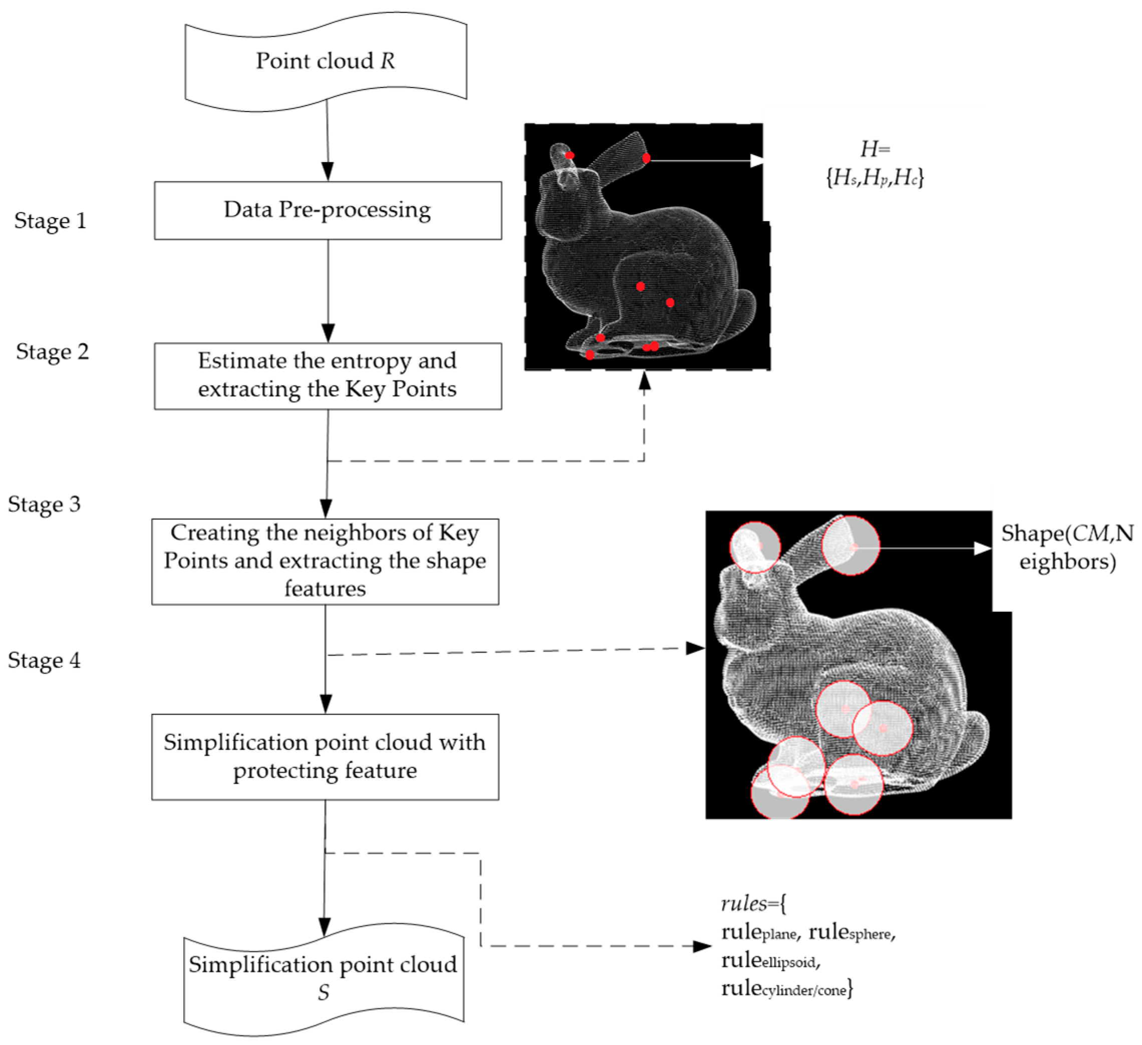
where R is the data set of the point cloud, which is the full set of data, ; H is the set of point cloud simplification entropy; PCMM is the set of point cloud matching models, which is composed of natural quadric shape models (e.g., ellipsoid, cylinder, cone); C is the data set that is reduced by FPPS; S is the data set that is saved by FPPS, which is C’s complementary set; and rules represent the mapping rules, which are set in terms of the PCMM.
The purpose of FPPS is to divide the full set, R, into two subsets, S and C. Ideally, set S includes all of the geometric features, and set C is the redundant data. So, H describes and measures the geometric features, and then the elements in set R can be mapped one-by-one to the tuple H. PCMM is independent of the point cloud set R and is the regular point cloud shape’s model set. The similarity between PCMM and subset R is useful for recognizing the local shape features in the FPPS. So, the mapping of PCMM and subset R is one-to-many. By comparing the similarity, the rules can be inferred, and rules are important for simplification in FPPS, for example, the adjustment of the self-adaptive reduction ratio.
The proposed point cloud simplification framework is composed of four stages, as shown in Figure 1. The point clouds are collected by the laser scanner, which only provides the position of the points. Thus, the data attributes are scattered and simple. No topological and relative positional relations can be found in the data. Most of the point clouds just have the points’ coordinates. Obviously, the simple data attributes are deficient, which makes data simplification with geometric features difficult. FPPS tries to retrieve more geometric features. In FPPS, the first stage of point cloud simplification is data pre-processing, which is able to estimate the normal vector of point clouds (see Section 2.1). Then, we divide the geometric features into three types and estimate each of them using the entropy which quantifies the geometric features. Like the criterion, the entropy is used to extract the key points. Thus, the key points will include more information about geometric features in the second stage. Additionally, the simplification entropy is defined (see Section 2.2). In the third stage, the neighbors of key points are created, and then the point clouds are divided into different segments, following which we evaluate the shape features of each segment. In the fourth stage of point cloud simplification, we match the shape features of each segment to the natural quadric surface in PCMM. Based on the shape features, we set the rules and simplify the point clouds (see Section 2.3 and Section 2.4).
2.1. Data Pre-Processing
2.1.1. Data Collection and Normalization
Today, there is a diverse range of laser scanners, which are the leading equipment for point cloud collection, e.g., spot scanner, single linear scanner, and multi-linear scanner. The source data gathered by the laser scanner can deduce the object’s depth value. However, the data types used are different. As an example, Kinect provides six data sources: ColorFrameSource, InfraredFrameSource, DepthFrameSource, BodyIndexFrameSource, BodyFrameSource, and AudioSource. The depthFrameSource channel is selected to gain depth data and this is converted to point cloud (*.pcd). Another common device is Lidar (Light Detection and Ranging). The format of Lidar data is the LDEFS (Lidar Data Exchange Format Standard), whose file extension is “.las”. The “point data” is extracted in LDEFS and converted to point cloud (*.pcd). In this paper, the point clouds data set is indicated as , , where points are addressed with a constructor notation p(x,y,z) and n is the size of data set R. Because of the uncertainty of the measured object scale, it is difficult to find a suitable view port and show the complete object model for the user. During the pre-process point clouds, data normalization is carried out. The data normalization procedure is executed as shown in Equation (1):
2.1.2. Direction Adjusting
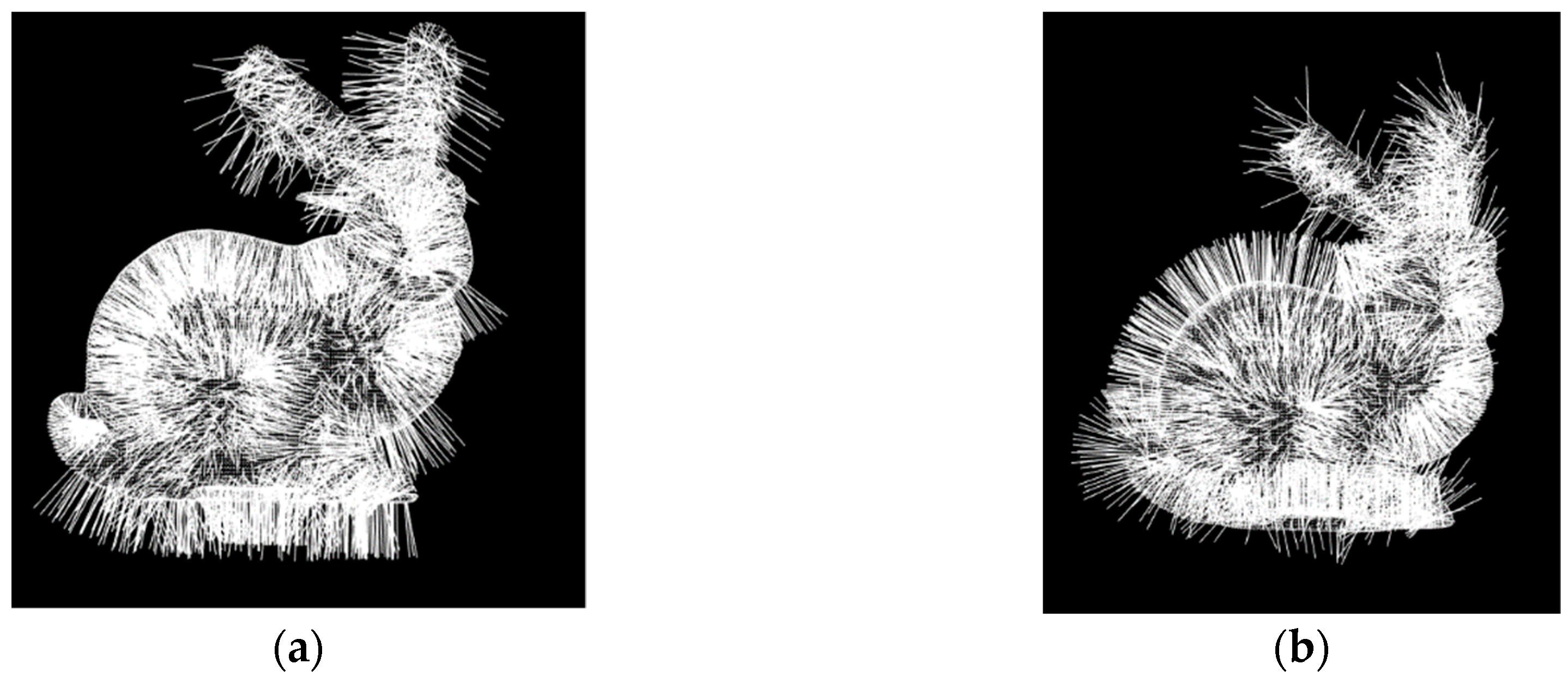
Using the PCA (principal component analysis) algorithm, three orthogonal directions which indicated the vectors, V1, V2, and V3 can be estimated, and then the normal vector can be evaluated using PCA, as shown in Figure 2a. Then, the normal vector’s direction is adjusted to make it consistent [39]. The result of this direction adjustment is shown in Figure 2b.
2.2. Simplification Entropy of Key Points
All the elements in key points belong to the data set of point cloud, R, which means that the data set of key points is a subset of R that includes the critical geometric features which should be measured and quantified. The goal of FPPS is to select suitable key points which are critical for set S. Therefore, in FPPS, the entropy is imported into point cloud simplification for geometric feature quantification, which is defined as simplification entropy, and used to determine the information about object features, e.g., scale-keeping feature, profile and curve feature.
The first type of simplification entropy, which measures the point’s scale-keeping capability for geometric features, is called the scale-keeping simplification entropy. The second type of simplification entropy describes the degree of importance of points on the surface boundary, which is called profile-keeping simplification entropy. The last type of entropy quantifies the surface curve’s information that is hidden in the points; this is called curve-keeping simplification entropy. According to the simplification entropy of point cloud, the key points can be found, and the key points are important for preserving geometric features.
2.2.1. Scale-Keeping Simplification Entropy
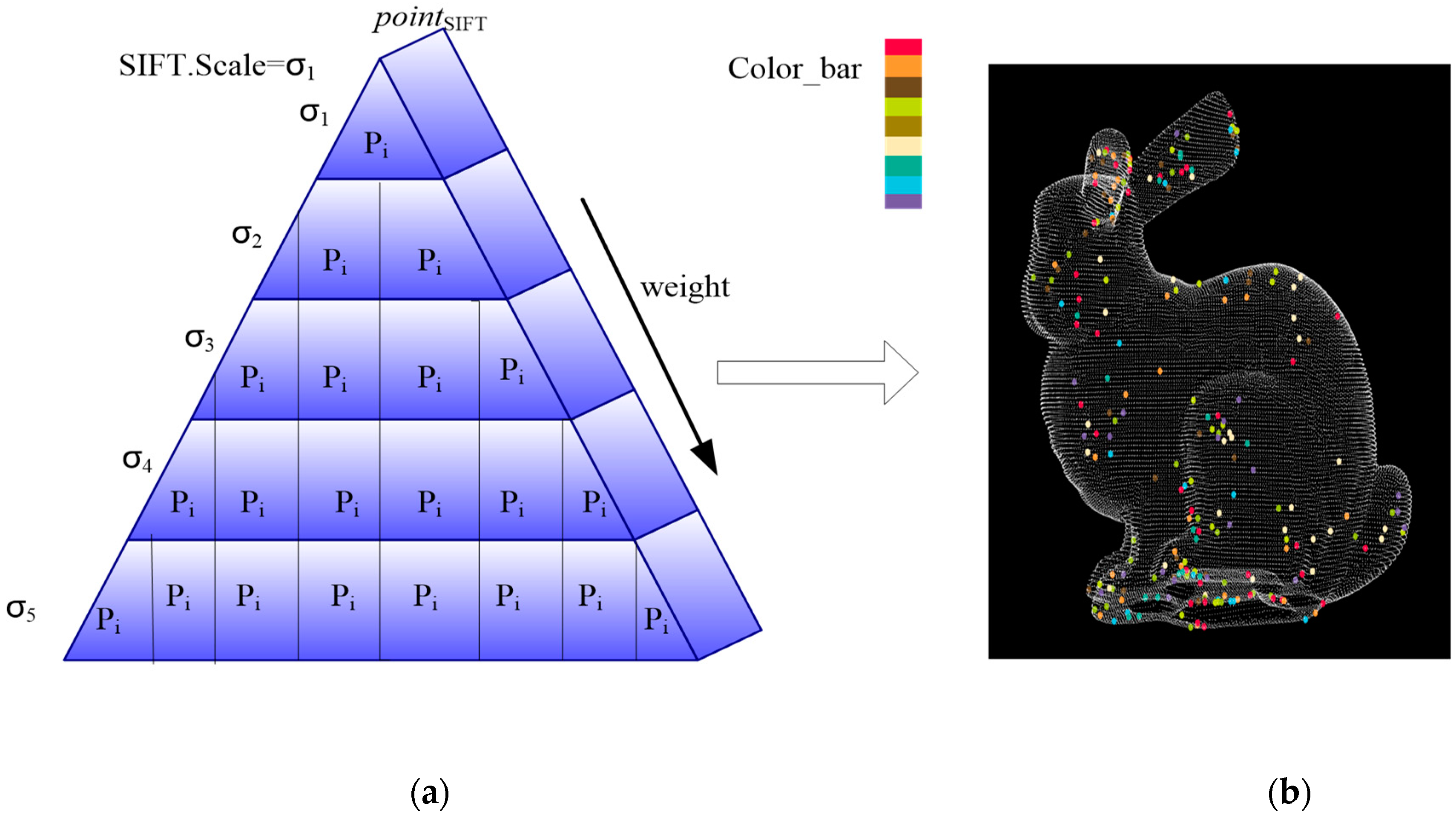
Inspired by the SIFT (scale-invariant feature transform) algorithm [40], for scale-keeping, the multi-layer point cloud voxel grids are created by voxelization, like a pyramid. Each layer in the pyramid is composed of the pointSIFT with the same scale value, SIFT.Scale = σ. The pointSIFT is the point set that is the local DOG(difference of Gaussians) optimum in one layer with SIFT.Scale = σ:
where R is the data set of point cloud; is the ith element in R; is the scale value; and is the DOG of .
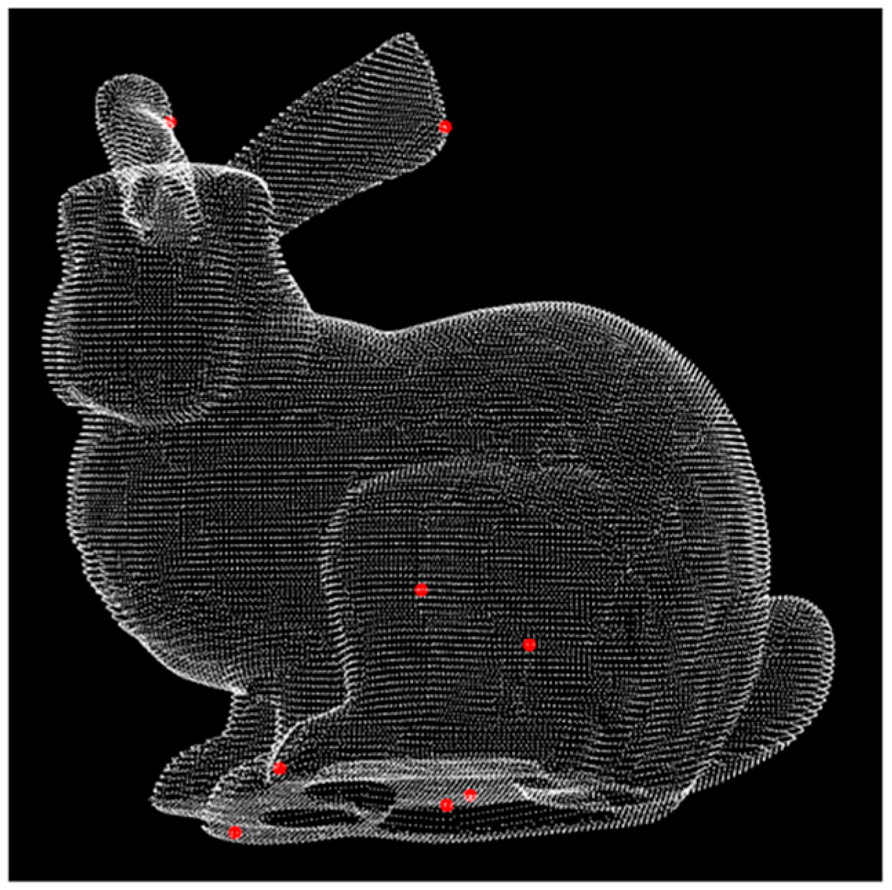
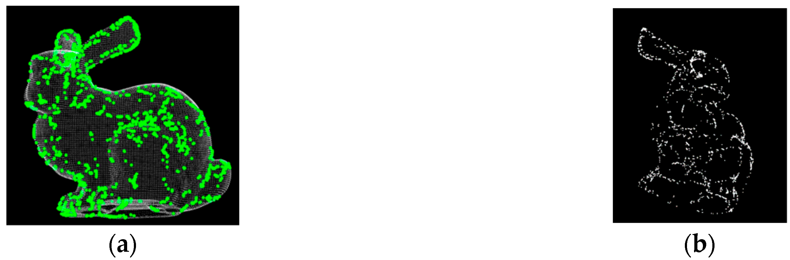
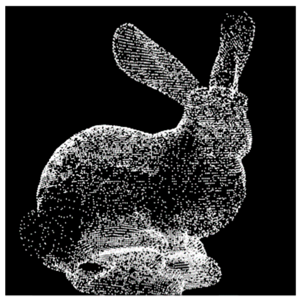
Taking the bunny data set [41] as the example, the pointSIFT in one layer of the pyramid is instantiated in Figure 3. The red points are the pointSIFT and . The size of the pointSIFT is 8, and the result can be seen from the red points in Figure 3.
Then, the of the multi-layers is extracted like a pyramid, as shown in Figure 4a. The extracted elements are shown in Figure 4b with the different colors. The ‘Color_bar’ in Figure 4b shows the element in different layers of the pyramid.
The elements in one layer with SIFT.Scale = σ represent the local optimum. Therefore, the distribution of elements in the layer is even, as shown in Figure 3. However, as shown in Figure 4b, the elements in different layers show an aggregation phenomenon and the Euclidean distance of points in is short. So, we think that the close elements in different layers have a lower capability to express the scale-keeping feature; therefore, a lower simplification entropy is set in FPPS. For the accuracy simplification entropy, the weight of the simplification entropy is set as shown in Equation (3).
where represents the layer number of the pyramid, and represents the cardinality of .
The is the probability value of in the full set R. Thus, the number of key points for scale keeping is less than . Assuming that the number of key points for scale keeping is , the points need to be saved by FPPS. Then, the probability of is limited in the interval [0, ). We set the weight of scale-keeping simplification entropy as the layer in the pyramid, and then points on the top of the pyramid have the biggest weight values; the points in the same layer are equally capable of describing scale-keeping information. The scale-keeping simplification entropy can be defined as follows:
2.2.2. Profile-Keeping Simplification Entropy
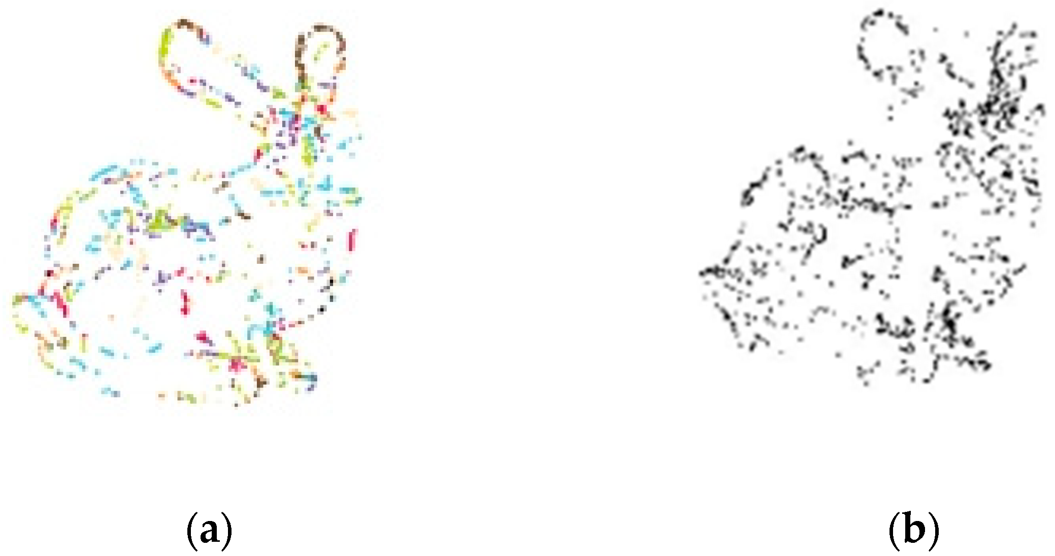
Profile-keeping simplification entropy is the value that can measure the profile information on the surface. It is generally known that the profile is important for the description of geometric features. The profile of the point cloud can be seen as the boundary around them. Thus, the boundary has to be treated as a special data type during point cloud simplification, and it should be protected and stored in the result set, S. Dense point cloud has a similar vector angle and density values within a small enough area. In the small area, the points with minimum density are considered as the boundary of this area. To improve the algorithm’s effect, the minimum angle of the neighbor normal vectors is introduced into the boundary feature extracting algorithm. Taking the “bunny” data set as an example, the boundary feature data are retrieved and are shown in Figure 5.
We found that boundary points that are close to each other have a similar feature description capacity. Thus, the data entropy becomes smaller for close data. Then, the distances among boundary data points can be set as the parameters of profile-keeping simplification entropy. In order to verify this, we created some boundary clusters by applying the Octree boundary clusters, which are shown in Figure 6a. Additionally, the centers of clusters are shown in Figure 6b. These clusters of boundary data are created, and each cluster is color-coded in Figure 6. Each cluster is assigned the same simplification entropy value. Then, the total entropy of the boundary data, which is divided into one cluster, is identical. Moreover, the boundary points in one cluster are different, and they are proportional to the distance from the cluster center.
The key points which provide the rich boundary features, form the subset of R. Assuming that shows the percentages of the subset’s size in the full set, is the probability of a subset including the profile-keeping feature and needs to be preserved in FPPS. Therefore, the probability of boundary data is in the interval [0, ). Every cluster is considered to have the same capability for profile-keeping feature description, and the same simplification entropy value. The variable is set as the number of clusters. All boundary data in one cluster have the same simplification entropy value, that is, . Then, based on the distance from the cluster center to the point data, we set the weight of profile-keeping simplification entropy for each point in the cluster. The profile-keeping simplification entropy can be defined as follows:
where is the distance from the cluster center to .
2.2.3. Curve-Keeping Simplification Entropy
The curve intuitively has more influence on the geometric features. The curve value participates in the simplification through curve-keeping simplification entropy. In the local area, the three principal vectors, which can be represented by , , and , are found by PCA (principal component analysis). Corresponding to the three principal vectors, the eigenvalues are represented as , , and , respectively.
We create the covariance matrix C of point cloud R:
where is the number of ’s neighbors; and is the centroid of .
Using the singular value, matrix C can be decomposed as:
is calculated by Equation (8):
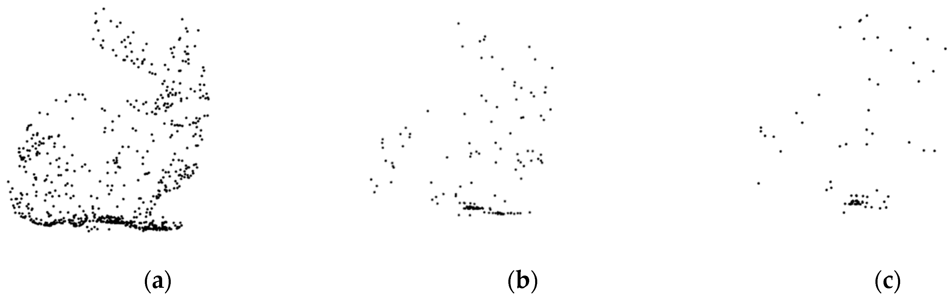
The value of reflects the curve of the surface. If the value of is bigger, the surface is sharper. Taking the “bunny” dataset as an example, the local maximum and minimum values of are extracted, as shown in Figure 7.
From Figure 7, we know that the value reflects the curve of the surface. Additionally, sharp surface features are important for the simplification. To protect the geometric features, most of the simplification algorithms consider that the sharper areas are important and should be protected to a large extent. However, in this paper, we consider the minimum of to also be important for preserving smooth geometric features, or else a lot of holes will be produced in the reconstructed surface. Therefore, we set a threshold , which is the number of key points required for curve preservation.
Figure 7 shows the feature points with different thresholds .
Using the Kd-tree with threshold , the neighbors of key points are created for curve surface features, which reflect the curve feature of the surface. When combined with the Gaussian kernel function, the curve-preserving simplification entropy can be defined as follows:
where is the threshold to control the scale of the feature points’ neighbors; and is the average of .
2.3. The Simplification Model Based on the Shape Feature
In the process of reverse reconstruction of point clouds, due to the dispersivity of point clouds, it is difficult to find the relationship between the data sets and to estimate the geometric features of the point clouds. In different application fields, there are different focuses on geometrical features. Therefore, there are many descriptions of the geometrical features of point clouds, for example, normal, curvature, flat, peak, cylinder, minimal surface, and ridge, etc. The local geometric features are important for simplification, especially because having an accurate description of them directly determines the effect of the reverse reconstruction or measured precision. To accurately describe the geometric features, the shape feature is brought into FPPS and estimated and measured by the point clouds matching model (PCMM).
In order to find the point clouds shape features during the process of data simplification, this paper provides PCMM based on the conicoid. By matching the shapes of features between the raw point clouds and PCMM, the data can be simplified by a certain shape feature, while the effective data feature can be reserved.
Because the conicoid has been clearly described, and the shape feature of the conicoid can be completely controlled, we created PCMM based on the conicoid, as shown in Equation (10).
It is assumed that there is a point data set , and that belongs to the raw point cloud R, that is
If point p is considered to be the one element in PCMM, the point meets function in Equation (10).
Because the whole conicoid model database is too large, the matching operation between the model and data sets consumes more time. Therefore, we revised and simplified the PCMM. For the convenience of algorithm implementation, in this paper, the data model is simplified based on the Nature Quadrics Model (NQM). The NQM model includes ball, ellipsoid, cylinder, and cone shapes. Additionally, the plane is an important and frequently used model in reconstruction, and the plane satisfies Equation (11):
So, in this paper, the plane and the NQM are considered the basic models in the data matching model database PCMM. Using the NQM and the plane, the PCMM can be simplified considerably. Based on the PCMM, similar and redundant data can be retrieved, and then the simplification algorithm can be implemented by reducing the data with similar shape features. Then, to exploit the points/area with similar shape features, a shape operator, , is used. The neighbors of point cloud are denoted as , and is one key point. The data matching model database is PCMM, and the shape measurement between and PCMM can be computed as shown in Equation (12). The function is the estimation value of the shape feature, which is computed by the distance of the point q and the projection of the point q. Thus, the function is important to the shape information description, and the value of is proportional to the distinctiveness of the shape feature:
where is the scale of neighbor points; is the function for the estimation of the shape feature; is one element in the ; and is the projection of in PCMM.
2.4. Simplification Rules
The simplification entropy is used for estimating the geometric features of point clouds. When combined with the shape features, we define the simplifying rules, which are shown in Table 1. In this paper, according to the different simplification actions, we divide the simplification rules into four parts, i.e., the rule for planes, the rule for spheres, the rule for ellipsoids and the rule for cylinders/cones. According to the rules, adaptive adjustment of the simplification ratio can be accomplished, and eventually the point clouds data is divided into two categories: the reserved set and the reduced set .
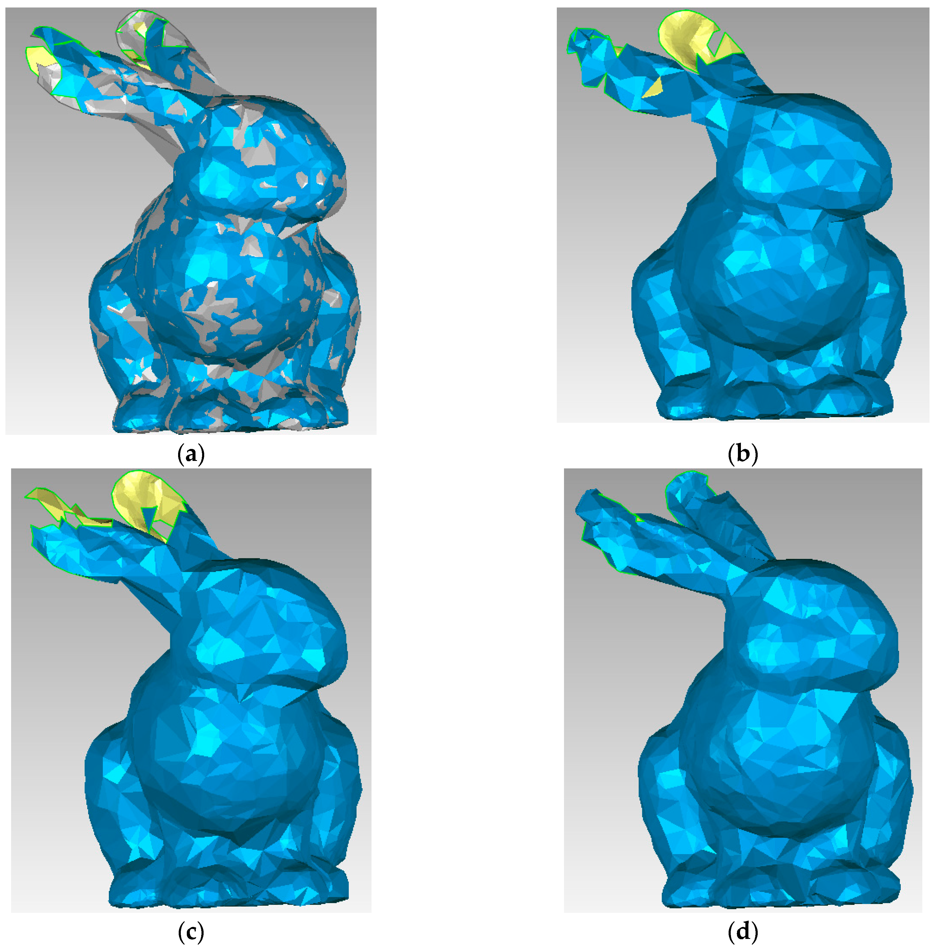
(1) Rule for planes: Because planes are flat and the location information is important for the local plane, we set the rule and actions for planes by creating voxels. The simplification algorithm is implemented by using voxelization at resolution , which is represented as the symbol , to downsample the point cloud. The center and boundary points are useful for determining the location information of a plane. The is the central voxel in the plane, and the is the function to extract the boundary. Based on actions of (b) and (c) in the first row of Table 1, the center and boundary of the plane are selected and saved in S. The point cloud R of the standard plane are shown in the third column of Table 1, and the simplified point cloud S are shown in the last column of Table 1.
(2) Rule for spheres: If the area is matched with a sphere, the point cloud curvature is similar in this area. The radius and the center of the sphere are important location information for the sphere. The center is saved in S according to the action in the second row of Table 1. As for the sphere’s shape feature, we consider that the points which are not satisfied by the sphere function are also important. The points are classified into three types, i.e., the points which are sharper than the sphere (), the points which are next to the sphere() and the points which are more smooth than the sphere (). By the way, the is the curvature of the sphere; the is the variance of point clouds’ curvature; the and are the threshold for the classification. The example of standard sphere simplification is shown in the second row of Table 2.
(3) Rule for ellipsoids: If the area is matched with an ellipsoid, the shape features can be described as the center and the three axes of the ellipsoid. The degree of importance of the points for shape-keeping changes with the simplification entropy. Thus, the voxels are created with the variable . is the average of hs (i.e., the scale-keeping simplification entropy), hp (i.e., the profile-keeping simplification entropy), and hc (i.e., the curve-keeping simplification entropy), which are computed by the Equations (4), (5) and (9), respectively. The simplification algorithm is implemented by using voxelization with variable resolution ,(i.e.,) to downsample the point cloud. The boundary and the center of the ellipsoid are also important to the location of the shape features. Thus, the boundary is extracted by the function ; and the center of the ellipsoid can be implemented by the action . The example of standard ellipsoid simplification is shown in the fourth row of Table 1.
(4) Rule for cylinders/cones: If the area is matched with a cylinder/cone, the top and bottom of the cylinders/cones is important to shape-keeping. The distance () between points and the axis of the cylinder/cone can be seen as the criterion by which the location of a point relative to the cylinder/cone is judged. is the threshold of distance, and the is the maximum of distance () in the last row of Table 1. The points are classified into two types during the point cloud simplification. The points which are next to the top or bottom of cylinder/cone, are simplified as the voxels at the fixed resolution . The points which are next to the body of the cylinder/cone, are simplified as the voxels at the variable resolution . An example of standard cone simplification is shown in the last row of Table 2.
3. Experiments and Discussions
3.1. Experimental Environment and Data Set
All experiments were performed on CA, US Intel (R) Core(TM) i7-3520M (CPU @2.90 GHZ, 8 GB memory, Windows 10 system). The code was written in the Visual C++ development environment, and the software platform used was QT5.6.2 + PCL1.8 + Visual Studio 2015.
The data set was managed using the MySQL database system and is shown in Table 2.
3.2. The Discussion of Self-Adapting Experiment Parameters
The purpose of this experiment was to discuss the influence of the experimental parameters on the simplification effect, which includes the simplification entropy and the neighborhood range of key points. Firstly, we assumed that the three types of key points could produce a balanced influence. Therefore, we set k as the number of key points and as the neighborhood range of each key point, in order to find the influences of k and on the simplification effect. The experiment used the constant c, where .
This experiment used c = 10,000. We adjusted parameters k and in the FPPS. The reduced point clouds were reconstructed, and the reconstructed surface is shown in Figure 8.
Figure 8 shows the reconstructed surface. As k increases, σ will shrink for a constant c, and the difference in the area of the triangle can be observed in Figure 8a–e. In particular, looking at Figure 8d,e, the triangles around the eyes and feet become obviously smaller and more refined, which shows that the reconstructed surface is smoother. A similar change in the triangle can be found around the joining of the bunny’s head with its ears. In contrast, the value in the fourth column of Table 3 (Number of Triangles) is bigger from top to bottom, which means that the triangles are refined. However, there are different phenomena in the fourth and fifth rows of Table 3. In the fourth row of Table 3, the values of “Number of Triangles” and “Size” columns, respectively, are 7145 and 4456, respectively, which are bigger than the values in the fifth row. This phenomenon reveals that the maximum value of k should be found. The maximum value of k provides the balance between the satisfied simplification result and the time consumption of FPPS.
The simplified results from this experiment are shown in Figure 8. We list the parameters (k, σ) and simplification results (number of triangles, size of S and simplification ratio) in Table 2, which correspond to Figure 8a–e. In these experiments, the experimental parameter c was set as 10,000. When k increases, the number of key points becomes bigger; thus, the overall features of the object are well preserved. However, the process of extracting key points is time consuming. When σ shrinks, the scope of a local area becomes smaller; the local areas which are selected to analyze the shape features become smaller; and the local features of an object, especially the “corner” or “sharp” features, are well estimated. Furthermore, the different local areas selected will result in different simplification sizes and simplification surfaces, which are shown in Table 3 and Figure 8. In Table 3, we list the reduced triangle number and reduced point cloud size. The simplification ratios calculated from the reduced point cloud size and original point cloud size are also listed. The number of triangular faces is between 6346 and 7336, and the simplification ratio is distributed between 9% and 12.3% by the FPPS. So, the changes in the simplification ratio and the number of triangular faces is small. However, we can see from the reconstruction surfaces in Figure 8 that the surfaces are different, especially on the richer surface features areas.
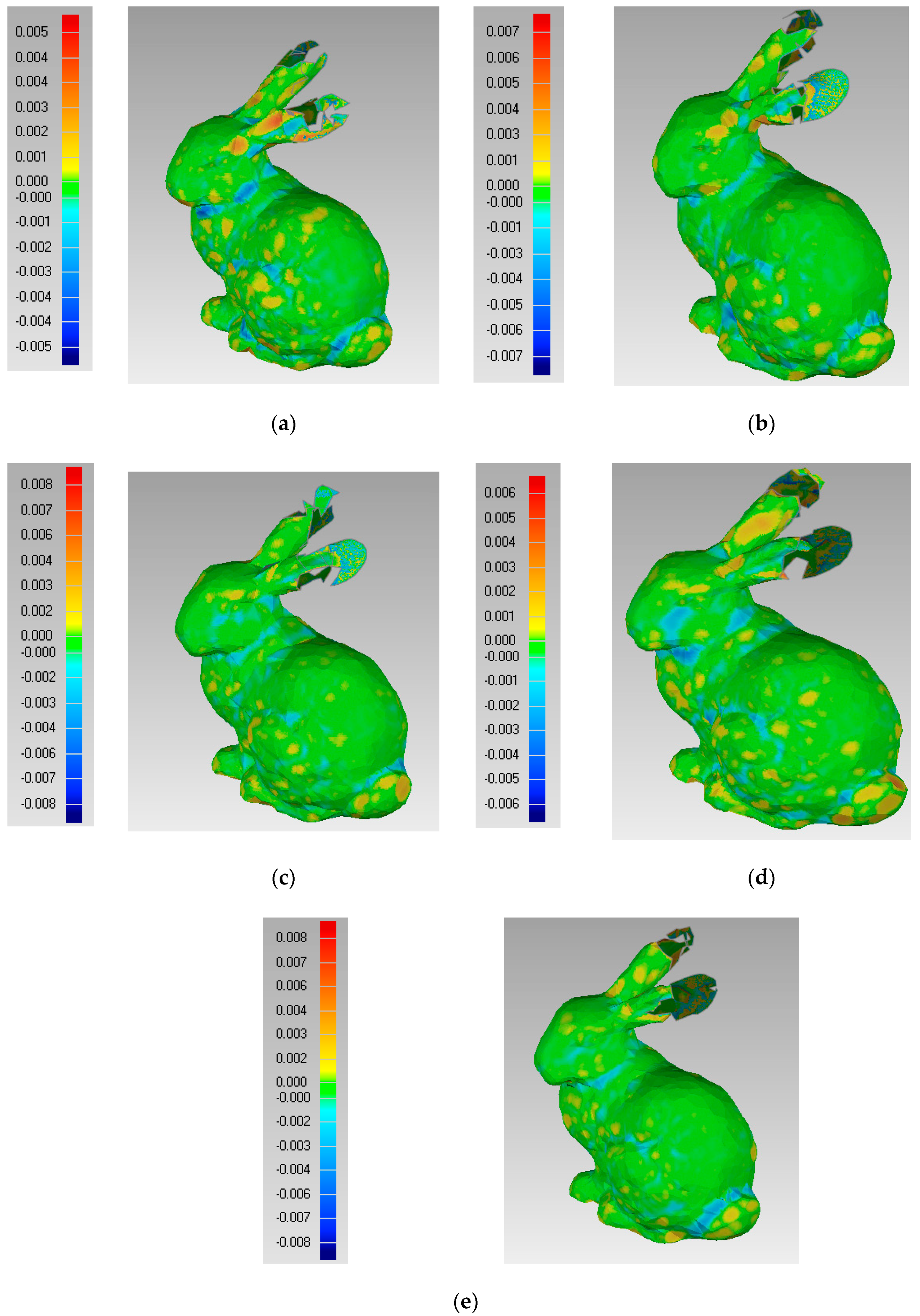
Then, we compare the effect of the reconstruction surface. The result of the comparison of two surfaces is shown in Figure 9; these are the surface reconstructed by S and the surface reconstructed by R.
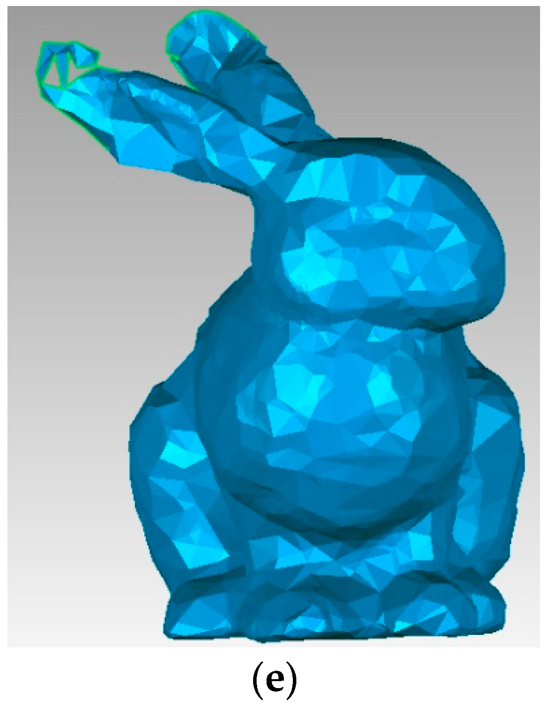
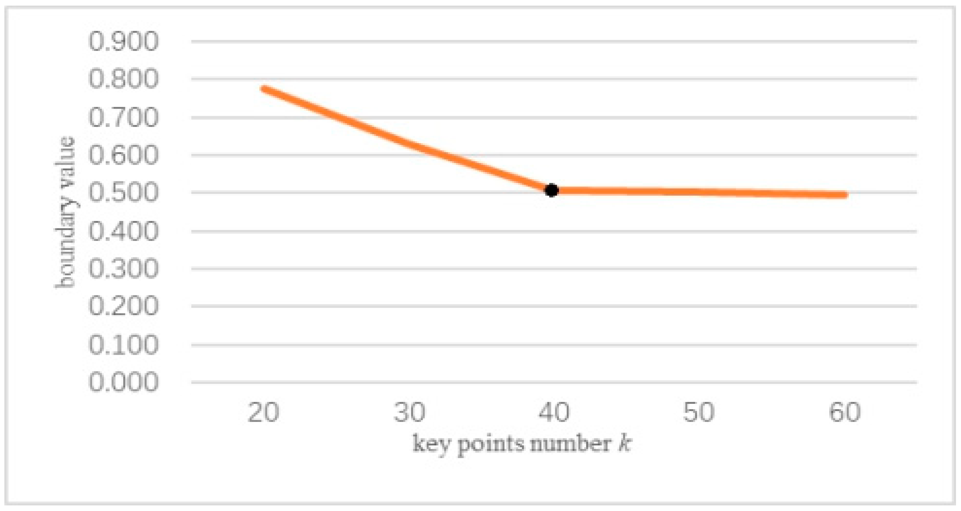
From Figure 9, we can see that if is the same and and are different, different effects on the reconstruction surface are obvious. In Figure 9, the left column is the deviation value of the two surfaces, which is noted by the color code. The experimental results show that and influence the protected features in FPPS. Compared to the deviation value of Figure 9a–e, the maximum deviation value of Figure 9a is in the range [−0.005, +0.005], which shows that experiment (a) produced a better effect. With a decrease in , the deviation range extends, and the simplification effect is worse. However, the range of Figure 9d is [−0.006, +0.006], which shows that if more key points are chosen, the simplification effect is revised. So, in order to find the suitable parameter , = 1 000 was fixed in experiment (a), and parameter was changed. The upper and lower limits of the deviation value in the simplification result comparison are extracted in Figure 10. In Figure 10, the boundary value is the absolute value of the upper and lower limits of deviation, and this is used to estimate the simplification effect. The boundary value changes with parameter , as shown in Figure 10.
From Figure 10, we can see that when parameter is set smaller than 50, that is 0.13% of the bunny’s size, the experiment produces a worse simplification effect. However, as increases, a greater burden on the experiment running time will be produced. Fortunately, the inflection point is shown in Figure 10. The experimental results show that the number of key points is greater than 0.2% of the number of points, the local area matches PCMM well, and the simplification rules fit the shape features. Eventually, a better simplification effect will be reached.
In this experiment, we assumed that the three types of key points were balanced in terms of their influences on simplification. Thus, parameter c should be set similar to the size of R, and the number of key points k should be set greater than 0.2% of the size of R for the simplification to be satisfied. For example, because the volume of the bunny data set is 35,947, parameter was set as 35,000, which is similar to 35,947. The lower limit for the number of key points was 70.
3.3. Comparison of the Simplification Effect with Other Algorithms
The aim of this experiment was to compare the simplification effect with other algorithms. In order to compare the geometric features in S easily, meshing for S is applied after FPPS. We used the same mesh algorithm, that is the greedy projection triangulation in PCL. Compared with the Poisson triangulation algorithm, the greedy projection triangulation reveals the geometric features on point clouds clearly. Except for FPPS, the other simplification algorithms—uniform-based [42], curvature-based [43], and grid-based [44] simplification algorithms—were performed by Geomatic at the same simplification ratio. In this experiment, we executed point cloud simplification on different data sets and analyzed the geometric features saved in S.
Because of the geometric features’ diversity, we classified the data sets into three types. The first type was natural objects, animals, or humans, which have a smoother surface with small sharp areas. The second type was machine components which usually have sharp corners and are absolutely flat. The last type was man-made data sets which are popular in VR (virtual reality).
3.3.1. Point Cloud Simplification for Natural Data Sets
The experiment used two classic data sets, bunny and dragon, which were provided by Stanford University. The size of the bunny data set was 35,947 points. From the first experiment, we knew that the experiment parameters could be set as = 35 000, = 70, and = 500 to provide satisfactory simplification results. By running the FPPS algorithm, the simplification data were obtained and are shown in Figure 11. The simplification ratio was 15.6%.
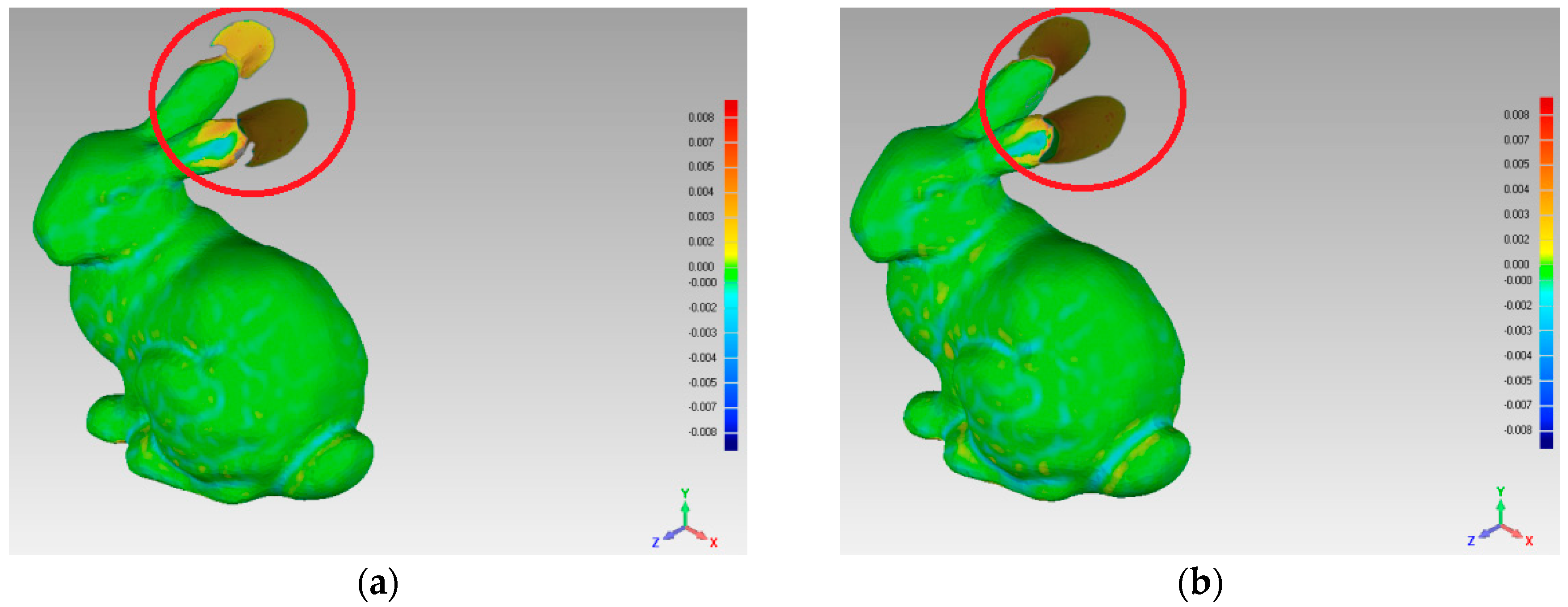
In order to compare the simplification effect of the two reconstructed surfaces, which were reconstructed by S and R, this experiment was implemented, the results of which are shown in Figure 12. When we estimated the deviation value between the two surfaces, the experimental results show that using the four simplification algorithms, the deviation value range is [−0.008, +0.008].
For the different areas of the bunny’s surface, we compared the simplification effects by four simplification algorithms. The simplification ratios of FPPS, uniform-based and curvature-based are set to the identical value, 15.6%. For the grid-based simplification algorithm, the point cloud simplification is implemented as the grid resolution. Therefore, the biggest interval distance of points in S equals the biggest interval distance by grid-based simplification. Subsequently, the simplification algorithm of grid-based simplification is 15.1%, which is close to 15.6%. For the ears area indicated by the red circle in Figure 12, the uniform-based and grid-based simplification algorithms produced large surface deviations. For the top of the ears, the gray areas show that all the points on one side are absent in the simplification result. The curvature-based simplification’s deviation value was less than 0.03, and just one ear has an obvious gray area in Figure 12c. Compared with the other algorithms, the FPPS produced a complete simplification effect in the ear area without a gray area, as shown in Figure 12d, and there was no large hole in the reconstructed surface. For the eye area, the uniform simplification produced an ambiguous reconstructed surface, and the eye area was difficult to recognize from other areas. The grid-based algorithm showed a more refined effect around the eyes than uniform-based simplification. The curvature-based and FPPS algorithms showed the best effects around the eye position. Relative to the ears and eyes, the body surface of the bunny was smoother. For the body area, the uniform-based algorithm was similar to the original surface, and the curvature-based, grid-based, and FPPS algorithms produced more deviation areas.
According to the experimental results mentioned above, for the FPPS algorithm, the simplified data loses surface precision, although the error is small and acceptable. Especially for the feature-rich area, surface holes and large deviations are less frequent occurrences. For the relatively smooth area, FPPS performs better than the grid-based and curvature-based algorithms, but the uniform-based algorithm shows the best effect. In addition, FPPS can protect the boundary data well with no large surface deviation, e.g., in the ear and tail areas.
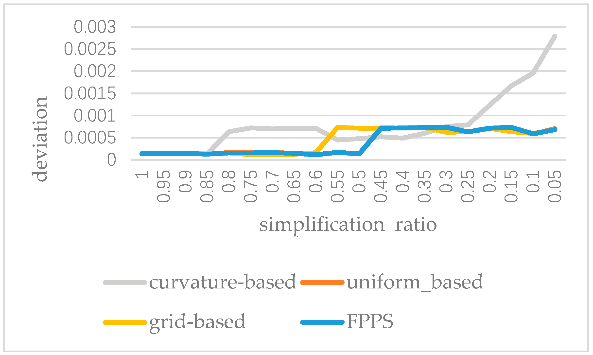
In order to analyze the stability of FPPS, we applied the four simplification algorithms to the “bunny” and implemented 20 groups of tests. After the execution of the 20 groups of tests, the deviation of the experimental results is recorded with the decrease in the simplification ratio, as shown in Figure 13. From Figure 13, we can see that the FPPS is a stable simplification algorithm. However, when the ratio is decreasing, the data volume is too small to present a satisfactory effect caused by the curvature-based algorithm. In Figure 13, the curve of uniform-based simplification is masked by the curve of FPPS, because for the “bunny” the stability of the uniform-based algorithm is similar to that of FPPS.
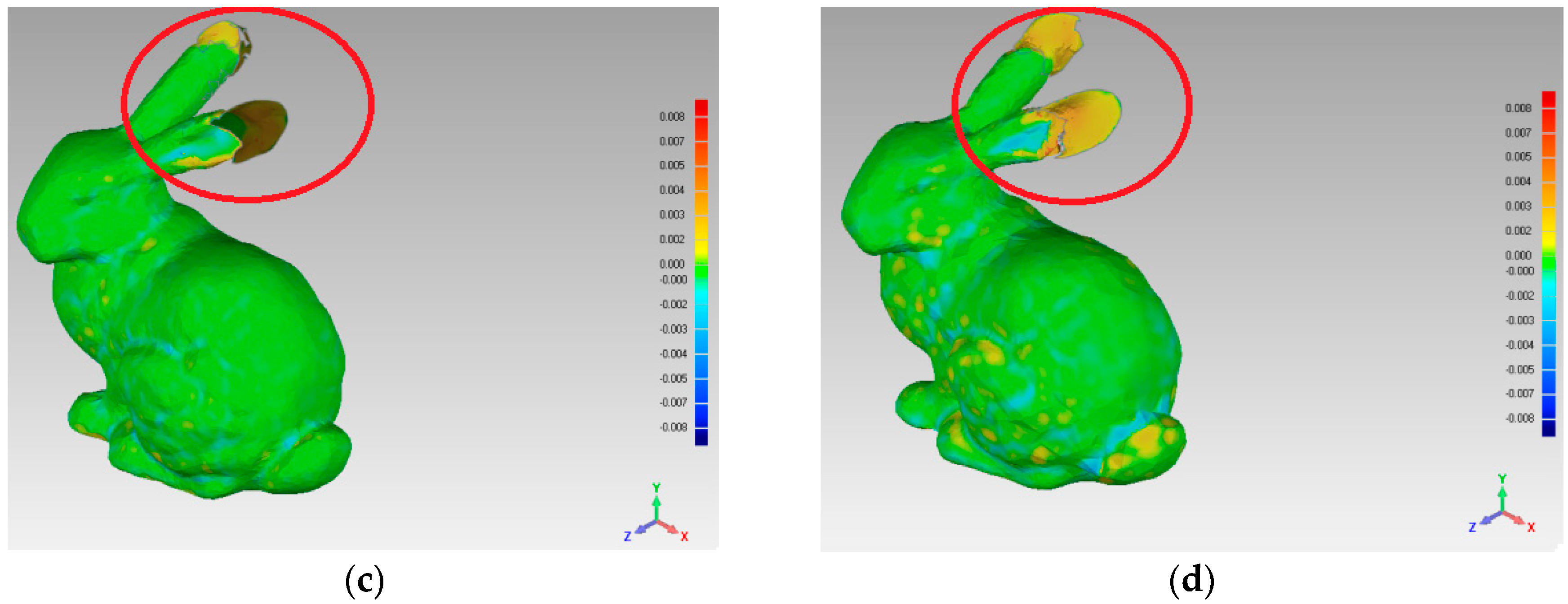
In order to further test the simplification effect, we also performed the simplification algorithms on the dragon data set. The dragon data set size is 437,645 points. When experiment parameter c is set to 400,000, the simplification ratio is 49.4%.
The simplification effects of the four algorithms are shown in Figure 13. The same simplification ratio, 49.4%, is applied to curvature-based and uniform-based algorithms. In addition to this, the simplification ratio of grid-based simplification is 49.5%. The experimental results show that when the FPPS or uniform-based simplification algorithm is used, the deviation value range is [−0.006, +0.006], which is narrower than that of other simplification algorithms, suggesting that these algorithms are superior to the other algorithms.
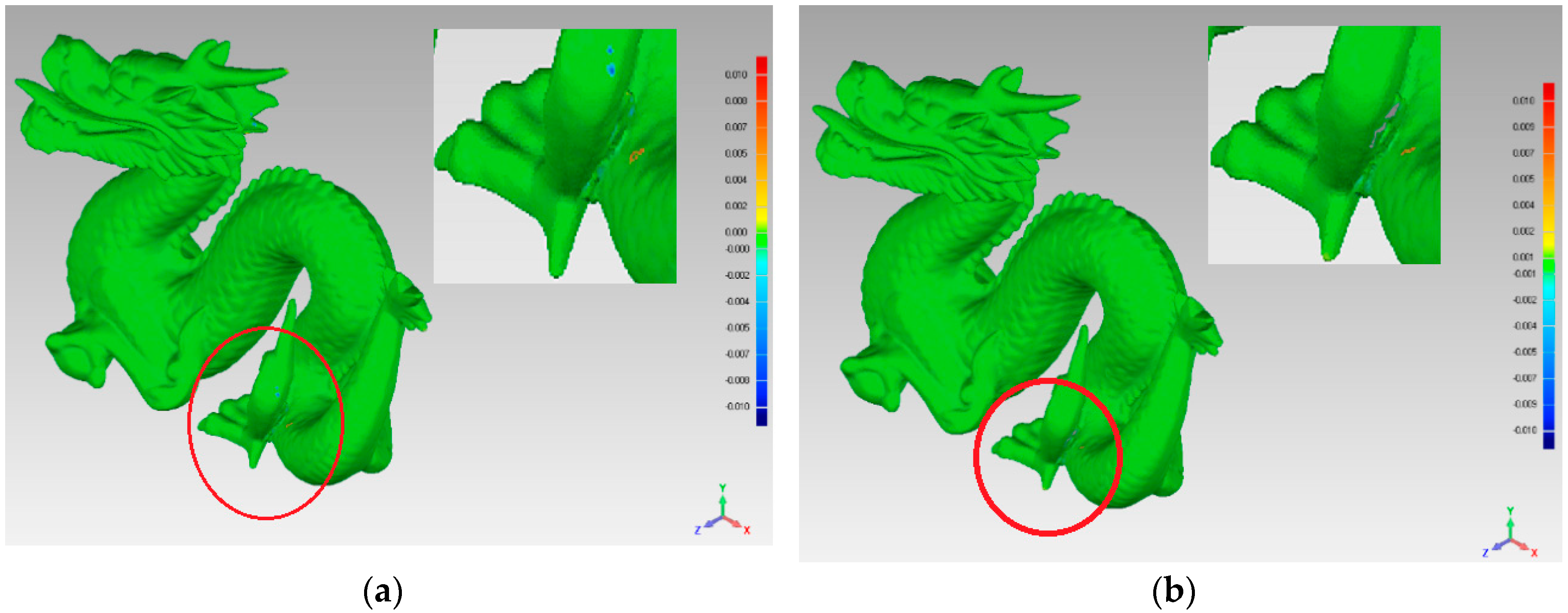
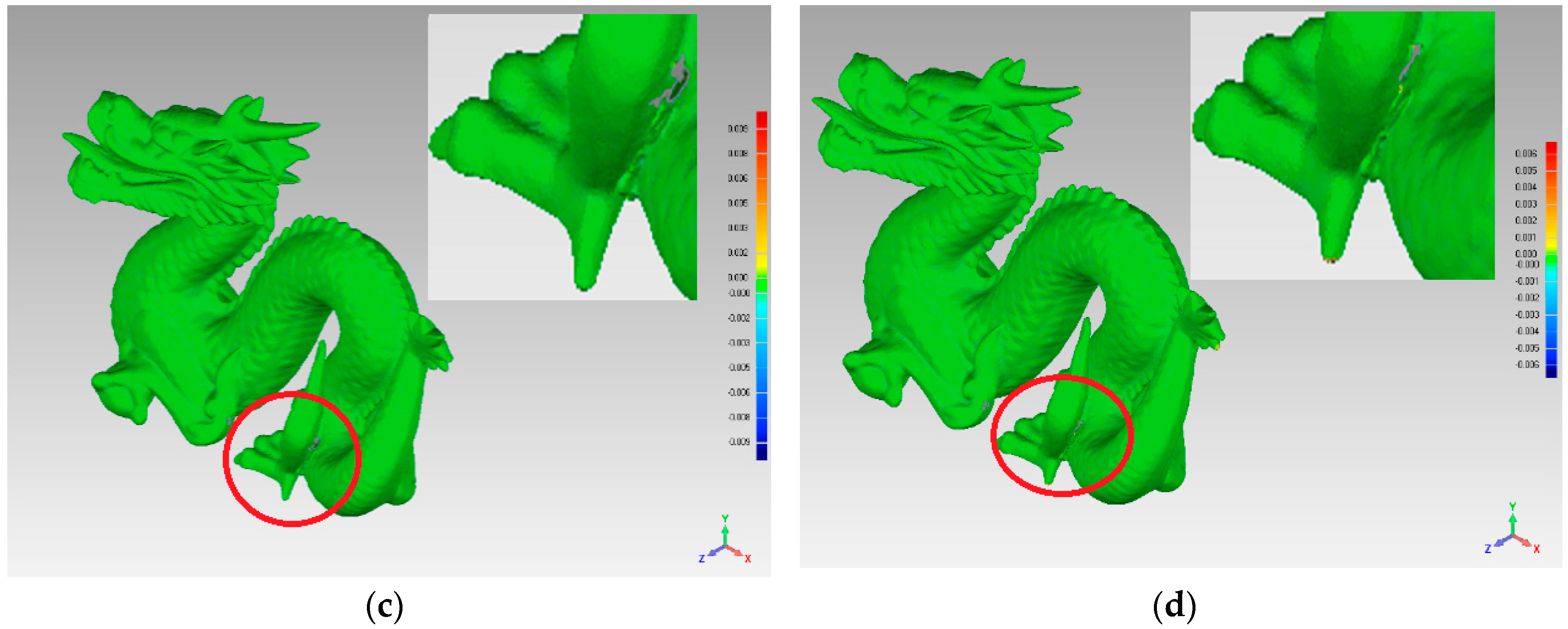
In order to compare the simplification quality in detail, we amplified the partial area around the dragon’s foot, as shown as a sub-figure in Figure 14. The sub-figure in Figure 14a shows the biggest deviation by the red and blue areas; therefore, the uniform-based simplification algorithm produced errors in the corner areas. A similar problem is shown by the red area in sub-figure Figure 14b. Compared with Figure 14a,b, Figure 14c,d shows less deviation around the dragon’s foot, which means that the FPPS and curvature-based simplification algorithms produced optimal effects on the complex curved surfaces.
Relative to the machine component and man-made data, there are always smaller continuous changes on the natural objects’ surfaces. Applying the FPPS simplification algorithm to natural data sets is superior to the uniform and grid algorithms in data sets with rich features. Additionally, for flat surfaces, FPPS performs slightly worse than the uniform-based simplification algorithm.
3.3.2. Point Cloud Simplification for the Machine Component Data Set
This data set has an explicit and regular shape feature, which can be easily identified and matched by simplification rules. Therefore, theoretically it is suitable to use the FPPS algorithm for this type of data. The data set, experiment parameter, and simplification results are described in Table 4, and the responding reconstructed surfaces are shown in Figure 15 and Figure 16. In this experiment, the data sets, called “Fandisk” and “Turbine Blade”, were used. We set experiment parameter c based on the results of the first experiment, as shown in the second column of Table 4. For FPPS, the simplification ratios were 90.7% and 40.7%, respectively. Using the FPPS’s simplification ratio, we executed the uniform-based, grid-based, and curvature-based algorithms. The grid-based algorithm adjusted the simplification ratio based on the grid resolution. For the “Fandisk”, the grid resolution is set as 0.086. According to the grid resolution, the simplification ratio is configured as 89.9%; for the “Turbine Blade”, the grid resolution is set as 1.384, and the simplification ratio is 41.8%.
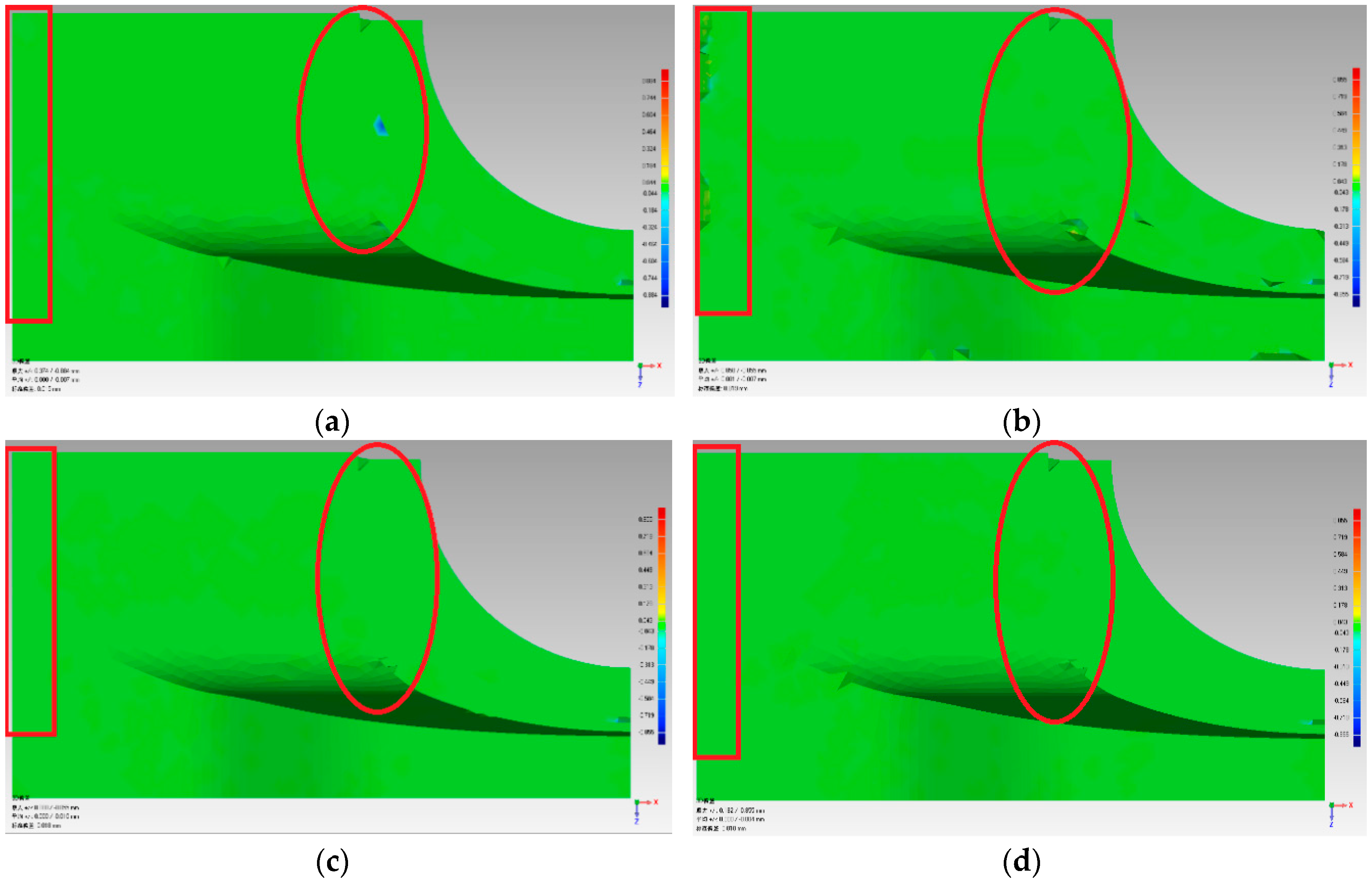
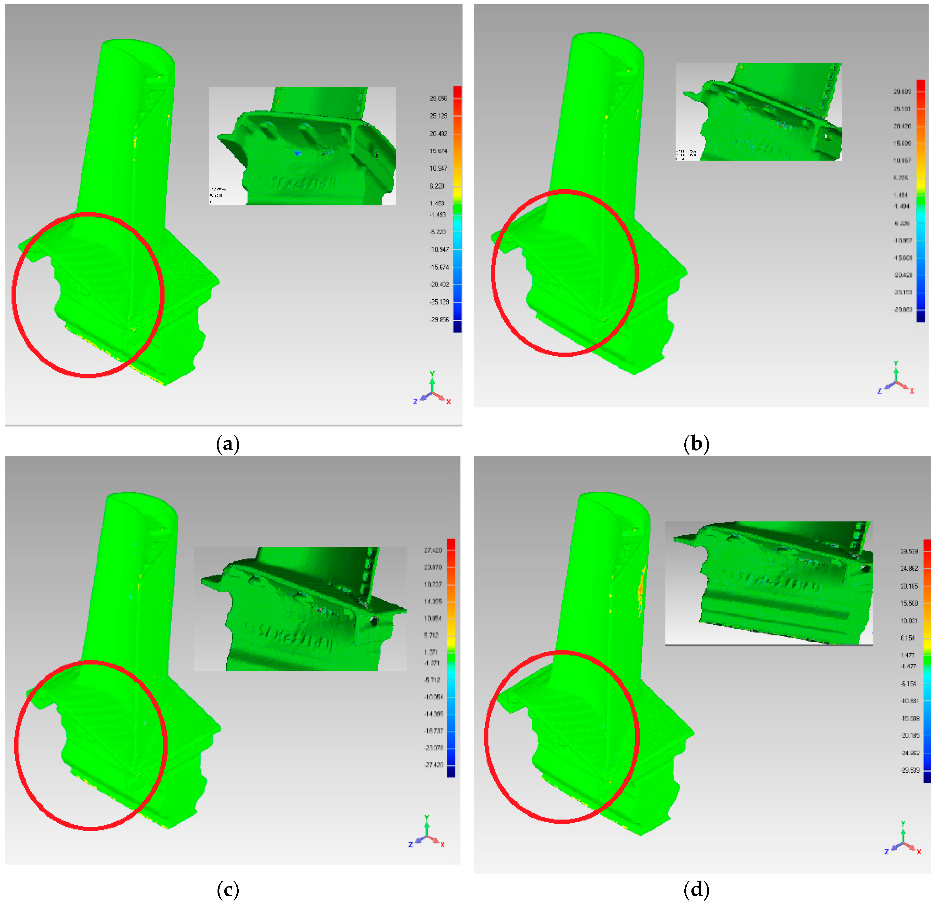
In Table 4, the deviation range and standard deviation are used to reflect the simplification quality. The simplification quality can also be observed in Figure 15 and Figure 16. The deviation range and standard deviation lists shown in Table 4 were less for the FPPS and curvature-based algorithms. Similar results can be seen in Figure 15 and Figure 16. From Figure 14, we can see that the FPPS had a better effect on the surface’s corner and boundary. However, for the flat and continuous area, FPPS had simplified the data with a bigger ratio, leading to greater deviation—these are the experimental results that we expected. In order to compare the effects of simplification, we added the red box and red circle in Figure 15. The red box is the boundary of “Fandisk”; Figure 15b shows an unregular boundary line, and the boundary surface in Figure 15a,c,d was reconstructed completely. When comparing with the red circle areas in Figure 15a–d, sub-figures c and d show the least deviation, which means that the curvature-based and FPPS algorithms preserve the surface features well. Furthermore, with the aim of analyzing the simplification effect, we list the sub-figure to show the details of the Turbine Blade data set in Figure 16a–d. The sub-figure is captured at another viewport, and the trademark can be seen in the sub-figure. Figure 16c,d are clearer than the other sub-figures; therefore, the curvature-based and FPPS algorithms produce less deviation from the original surface.
For the component data set, the comparison of experiment effects showed that the FPPS algorithm divides the surface into different regions and analyzes shape features, such as the boundary and curvature. During the process of the simplification algorithm, the regular shape was matched correctly, and the shape features were similar to those of the real surface, so the simplification effect was optimal, and the performance of the curvature-based algorithm was slightly lower than that of FPPS. However, faced with a wide range of surfaces that are similar to regular shapes, the uniform-based and grid-based simplification algorithms produce an unsatisfactory effect.
3.3.3. Point Cloud Simplification for the Machine Man-Made Data Set
The last data type is the man-made data set designed by a 3D tool, for example, 3DMax or AutoCAD. We used the data set “chair”, which was provided by Stanford University, to test the simplification effect.
The size of the Chair data set is 15,724 points. Based on the first experiment’s result, experiment parameter c was set as 15,000. Using FPPS, the simplification ratio reached 44.7%.
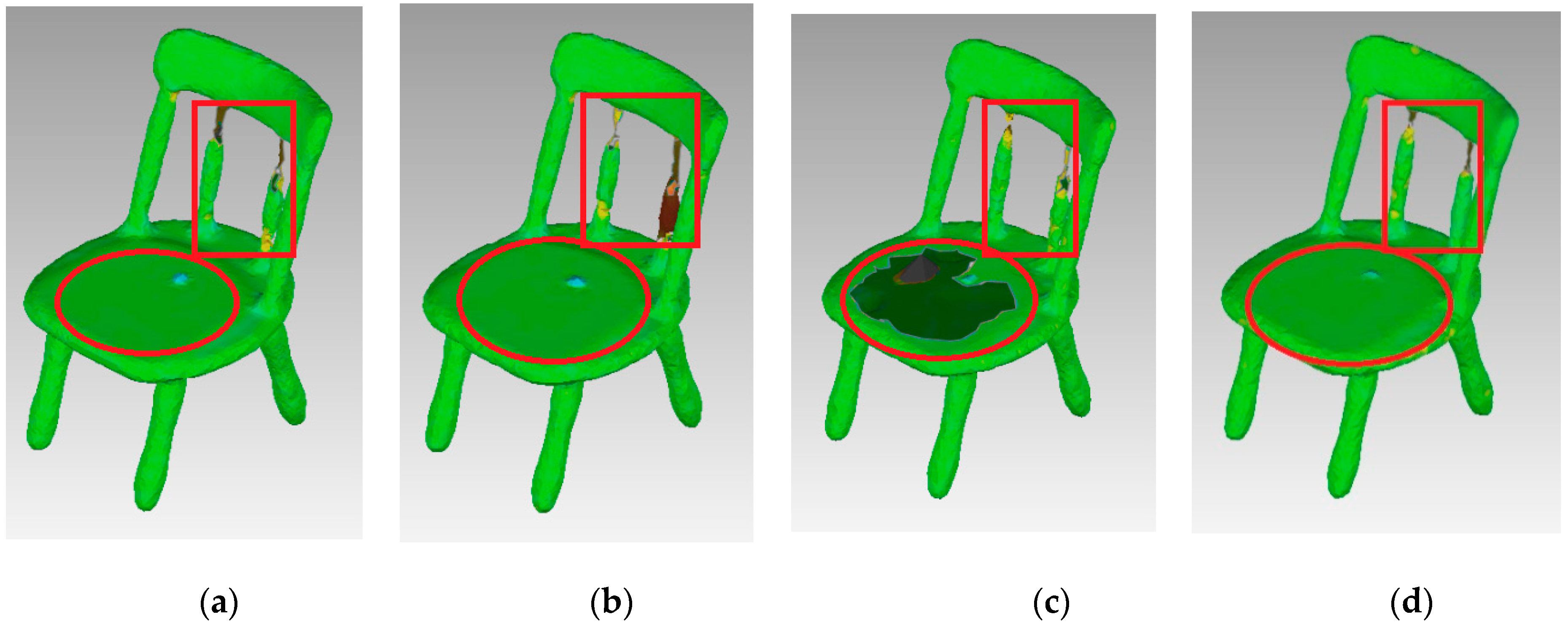
The experimental results are shown in Figure 17. As shown, the FPPS algorithm produced an optimally reconstructed surface. The chair’s surface was smooth, even though the corner lacks sharp features. As shown by the red circle in Figure 17, the surface of this area is flat. Figure 17c shows that the curvature-based algorithm is the worst one, as it provides insufficient data to express the surface. However, compared with the red rectangle area in Figure 17, this area is the joint in which the surface curve has an obvious difference. Thus, the curvature-based algorithm and FPPS produced surfaces similar to the original surface in this area and performed better than the uniformed-based and grid-based algorithm.
For man-made data, flat or sharp features are obvious on the surface. These obvious features are good for matching with regular shapes; thus, FPPS is suitable for man-made data.
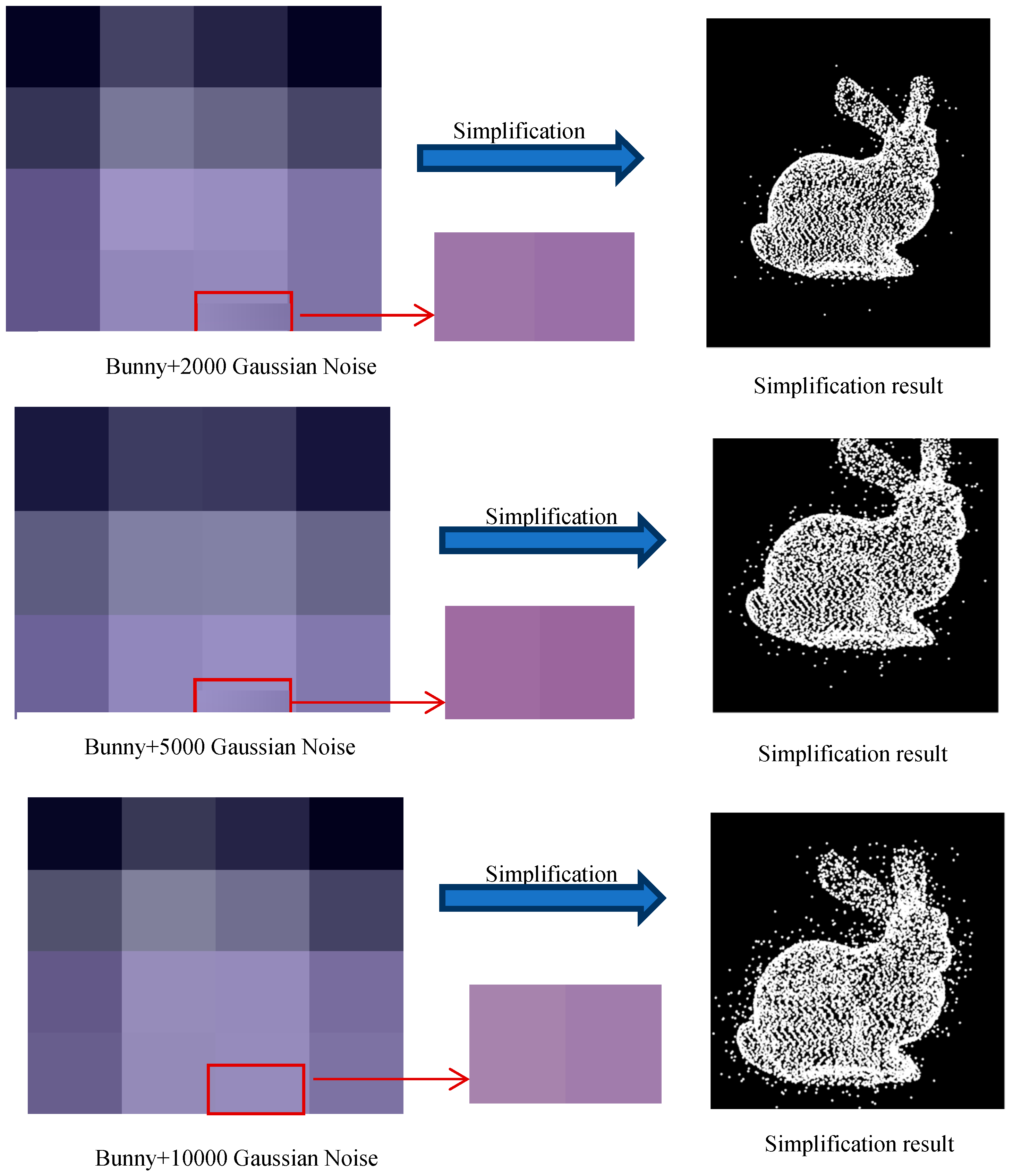
3.4. The Experiment for Robustness of FPPS
In order to test the robustness of the FPPS point cloud simplification algorithm, Gaussian noise was added to the “bunny” data set. The FPPS algorithm was implemented on the noisy data, and the algorithm results are shown on the right hand side of Figure 18. As can be seen in Figure 18, the noise was not removed at all by just using the simplification algorithm, although the noise was relatively reduced without the denoising algorithm. In order to verify the robustness of the algorithm, the experiment defined the noise simplification ratio, r:
where is the amount of noise; and is the noise that existed in set S.
In this experiment, we simplified the point cloud with Gaussian noise by K-means [17], curvature-based, random and FPPS. Then, the noise simplification ratio r was computed, as shown in Table 5. The experimental results show that FPPS can partially recognize noise, because of the shape matching operation. However, the other simplification algorithms are unable to detect noise at all.
3.5. Comparison of Algorithms’ Efficiency
In order to compare the FPPS algorithm’s efficiency with other algorithms, we carried out the point clouds simplification algorithm experiments on the same platform. The compared algorithms were grid-based, curvature-based, and K-means.
The type of CPU was CA, US Intel (R) Core (TM) i7-6820HQ (CPU @2.90 GHZ), and the main memory of the computer was 16 GB.
The IDE (integrated development environment) of the experiment was visual studio community 2015, and the UI (user interface) was designed by QT5.6.2. The PCL1.8 (point cloud library) was introduced into this experiment for the point cloud’s organization. The data sets used were Fandisk, Chair, and Bunny.
The grid-based simplification is designed and implemented based on the reference [42] and is improved in this experiment for effectiveness. The grid-based simplification created voxels at a specific resolution without geometric feature estimation, and computed the center of each voxel as the simplified point cloud. For the curvature-based simplification algorithm, we computed the curvature for each point by PCA. Then, the index of point clouds was created according to the curvature. In the experiment, when the specific simplification ratio was set, the bigger curvature was saved as simplified point clouds. For the K-means simplification algorithm, the point clouds and the number of clusters are the algorithm’s input, and the clusters are computed by K-means. Then, with the same simplification ratio for each cluster, the experiment can be implemented [17]. The experimental results are shown in Table 6.
The FPPS analyzes the geometric features of a measured object and computes the simplification entropy of point clouds. The entropy-extracted time complexity of the algorithm is O(N) and its space complexity is O(N). Then, FPPS compares the shape features with Natural Quadric Shape Models, and the algorithm’s time complexity is O(N). Therefore, as the last column in Table 6 shows, as the number of vertices in the point cloud increases, the memory usage and running time of FPPS become bigger.
Of the simplification algorithms, the grid-based algorithm has the optimal efficiency, without computing the geometric features. The K-means algorithm used the most system resources, including time and memory. The curvature-based and FPPS simplification algorithms, which are used for surface feature preservation, are more complex than the grid-based algorithm, and the running time of these algorithms is longer. The time and space complexity of the grid-based and curvature-based simplification algorithms is O(N), which is the same with FPPS.
4. Conclusions
This paper proposed a point cloud data simplification method, FPPS, which can reduce the point cloud volume and protect the geometric features hidden in the point cloud. In order to analyze the geometric features, FPPS divides the geometric features that need to be protected into three categories: scale, profile, and curve. In addition, the FPPS method quantifies the geometric feature information that is hidden in point cloud data and defines three types of simplification entropy: scale-keeping entropy, profile-keeping entropy, and curve-keeping entropy. The key points for the point cloud simplification algorithm are designed according to the simplification entropy. The experiments carried out as part of this study revealed that the key points include most geometric features. Neighborhoods are established across the key points, which are given special treatment to effectively maintain the surface features in FPPS. Then, based on the regular shape, FPPS simplifies the point cloud volume. We defined the point cloud matching model database, PCMM, and built simplification rules. FPPS was implemented by matching the neighborhood areas and PCMM, and had a better effect on the areas with a high similarity degree. The simplification parameters were adapted to local areas, and data hiding more geometric features were reserved. Finally, the experimental results showed that for the machine component and man-made data sets, the simplification effect is better, because of the high similarity in the regular shape features. In addition, FPPS can identify noisy data through shape matching, and the noise interference can be partially avoided.
Due to the limited conditions, PCMM has insufficient shapes. Therefore, when facing a natural data set, the similarity degree is lower, which leads to less improvement by the simplification effect. Furthermore, with FPPS, the measurement and analysis of features is more time-consuming than with grid-based and uniform-based algorithms.
In this paper, we not only proposed a reasonable implementation method for point cloud simplification (FPPS), but also used different data sets to validate the simplification effects of different simplification algorithms, which provides important information regarding the selection of a simplification algorithm. In addition, FPPS was used to measure the surface features by simplification entropy, which lays the foundation for point cloud shape analysis and is useful for point cloud object recognition.
In the future, we will expand the matching model database PCMM and the corresponding simplification rules to improve the adaptability of the FPPS algorithm. FPPS requires a lot of time for surface feature detection and shape matching, although it is better than the clustering reduction algorithm. Therefore, we will continue to work on optimizing the algorithm. We will try to optimize the special index of point clouds to improve the efficiency of data searching. Parallelized programming is another method to solve the problem of the algorithm’s efficiency. Using OpenMP and GPU, we have tried to introduce parallelization into FPPS.
Author Contributions
K.Z., S.Q., X.W. conceived the idea. K.Z. and X.W. established the point cloud simplification methodology as well as the formalized description of FPPS. S.Q. and Y.Y. developed the point cloud input, preprocessing, simplification and reconstructed system. K.Z. and S.Q. wrote the manuscript. Y.Z. and K.Z. designed the experiment to verify the stability of FPPS.
Funding
This research is funded by National Natural Science Foundation of China (No. 51271033), and supported by Special Program for Natural Science Foundation and Key Basic Research of Hebei Province of China (No. 18960106D), and Natural Science Foundation of Hebei Province of China (No. 2018208116), and Higher School Science and Technology Research Project of Hebei Province of China (No. Z2017008) and PhD Early Development Program of Hebei University of Science and Technology.
Acknowledgments
The authors also gratefully acknowledge the helpful comments and suggestions of the reviewers, which will improve the presentation. At the same time, we would also like to thank Stanford University for the 3D data set and the PCL developer.
Conflicts of Interest
The authors declare no conflict of interest.
References
- Pauly, M. Point Primitives for Interactive Modeling and Processing of 3D Geometry. Ph.D. Thesis, Federal Institute of Technology (ETH) of Zurich, Zurich, Switzerland, 2003. [Google Scholar]
- Shuai, Y.; Shuai, Z.; Li, D.S.; Wen, L.; Yu, Z.Y.; Yuan, L.W. Feature preserving multiresolution subdivision and simplification of point clouds: A conformal geometric algebra approach. Math. Methods Appl. Sci. 2018, 41, 4074–4087. [Google Scholar]
- Cabo, C.; Ordoñez, C.; García-Cortés, S.; Martínez, J. An algorithm for automatic detection of pole-like street furniture objects from mobile laser scanner point clouds. ISPRS J. Photogramm. Remote Sens. 2014, 87, 47–56. [Google Scholar] [CrossRef]
- Schauer, J.; Nuechter, A. The peopleremover—Removing dynamic objects from 3D point cloud data by traversing a voxel occupancy grid. IEEE Robot. Autom. Lett. 2018, 3, 1679–1686. [Google Scholar] [CrossRef]
- Mitra, N.J.; Pauly, M.; Wand, M.; Ceylan, D. Symmetry in 3D geometry: Extraction and applications. Comput. Graph. Forum 2013, 32, 1–23. [Google Scholar] [CrossRef]
- Hoppe, H. Progressive meshes. In Proceedings of the Conference on Computer Graphics & Interactive Techniques, New Orleans, LA, USA, 1 August 1996; pp. 99–108. [Google Scholar]
- Sanchez, G.L.; Esmeide, L.N. A linear programming approach for 3D point cloud simplification. IAENG Int. J. Comput. Sci. 2017, 44, 60–67. [Google Scholar]
- Tang, H.; Shu, H.Z.; Dillenseger, J.L.; Bao, X.D.; Luo, L.M. Moment-based metrics for mesh simplification. Comput. Graph. 2007, 31, 710–718. [Google Scholar] [CrossRef] [Green Version]
- Li, Y.; Zhu, Q. A new mesh simplification algorithm based on quadric error metrics. In Proceedings of the IEEE International Conference on Consumer Electronics, Berlin, Germany, 5–7 September 2016. [Google Scholar]
- Alexa, M.; Behr, J.; Cohenor, D.; Fleishman, S.; Levin, D.; Silva, C.T. Point set surfaces. In Proceedings of the IEEE Visualization, San Diego, CA, USA, 21–26 October 2001. [Google Scholar]
- Song, S.; Liu, J.; Yin, C. Data Reduction for Point Cloud Using Octree Coding; Springer International Publishing: Cham, Switzerland, 2017; pp. 376–383. [Google Scholar]
- Almeida, D.; Stark, S.; Shao, G.; Schietti, J.; Nelson, B.; Silva, C.; Gorgens, E.; Valbuena, R.; Papa, D.; Brancalion, P. Optimizing the remote detection of tropical rainforest structure with airborne lidar: Leaf area profile sensitivity to pulse density and spatial sampling. Remote Sens. 2019, 11, 92. [Google Scholar] [CrossRef]
- Schnabel, R.; Klein, R. Octree-Based Point-Cloud Compression; Eurographics: Los Angeles, CA, USA, 2006. [Google Scholar]
- Xie, Q.; Xie, X. Point cloud data reduction methods of octree-based coding and neighborhood search. In Proceedings of the International Conference on Electronic & Mechanical Engineering & Information Technology, Harbin, China, 12–14 August 2011. [Google Scholar]
- Benhabiles, H.; Aubreton, O.; Barki, H.; Tabia, H. Fast simplification with sharp feature preserving for 3D point clouds. In Proceedings of the International Symposium on Programming & Systems, Algiers, Algeria, 22–24 April 2013. [Google Scholar]
- Yuan, X.C.; Wu, L.-S.; Chen, H.W. Feature preserving point cloud simplification. Opt. Precis. Eng. 2015, 23, 2666–2676. [Google Scholar] [CrossRef]
- Shi, B.Q.; Liang, J.; Liu, Q. Adaptive simplification of point cloud using-means clustering. Comput. Aided Des. 2011, 43, 910–922. [Google Scholar] [CrossRef]
- Wang, Y.; Tang, J.; Rao, Q.; Yuan, C. High-efficient point cloud simplification based on the improved k-means clustering algorithm. J. Comput. Inf. Syst. 2015, 11, 433–440. [Google Scholar]
- Song, H.; Feng, H.Y. A global clustering approach to point cloud simplification with a specified data reduction ratio. Comput. Aided Des. 2008, 40, 281–292. [Google Scholar] [CrossRef]
- Li, T.; Pan, Q.; Liang, G.; Li, P. A novel simplification method of point cloud with directed hausdorff distance. In Proceedings of the IEEE International Conference on Computer Supported Cooperative Work in Design, Wellington, New Zealand, 26–28 April 2017. [Google Scholar]
- Alexa, M.; Behr, J.; Cohen-Or, D.; Fleishman, S.; Levin, D.; Silva, C.T. Computing and rendering point set surfaces. IEEE Trans. Vis. Comput. Graph. 2003, 9, 3–15. [Google Scholar] [CrossRef]
- Awrangjeb, M.; Siddiqui, F.U. A new mask for automatic building detection from high density point cloud data and multispectral imagery. ISPRS Ann. Photogramm. Remote Sens. Spat. Inf. Sci. 2017, IV-4/W4, 89–96. [Google Scholar] [CrossRef]
- Herraez, J.; Denia, J.L.; Navarro, P.; Yudici, S.; Martin, M.T.; Rodriguez, J. Optimal modelling of buildings through simultaneous automatic simplifications of point clouds obtained with a laser scanner. Measurement 2016, 93, 243–251. [Google Scholar] [CrossRef]
- Kim, S.J.; Kim, C.H.; Levin, D. Surface simplification using a discrete curvature norm. Comput. Graph. 2002, 26, 657–663. [Google Scholar] [CrossRef]
- Liu, K.; Chen, J.; Xing, S.; Han, H. Simplification of point cloud data based on gaussian curvature. In Proceedings of the IET International Conference on Smart and Sustainable City, Shanghai, China, 19–20 August 2013; pp. 11–14. [Google Scholar]
- Zhenguo, M.A. A point cloud simplification algorithm based on kd_tree and curvature sampling. Comput. Aided Des. 2010, 35, 64–69. [Google Scholar]
- Prakhya, S.M.; Liu, B.; Lin, W. Detecting keypoint sets on 3d point clouds via histogram of normal orientations. Pattern Recognit. Lett. 2016, 83, 42–48. [Google Scholar]
- Han, H.; Xie, H.; Sun, F.; Huang, C. Point cloud simplification with preserved edge based on normal vector. Opt. Int. J. Light Electron Opt. 2015, 126, 2157–2162. [Google Scholar] [CrossRef]
- Gospodarczyk, P. Degree reduction of bézier curves with restricted control points area. Comput. Aided Des. 2015, 62, 143–151. [Google Scholar] [CrossRef]
- Song, H.; Feng, H.Y. A progressive point cloud simplification algorithm with preserved sharp edge data. Int. J. Adv. Manuf. Technol. 2009, 45, 583–592. [Google Scholar] [CrossRef]
- Digne, J.; Cohen-Steiner, D.; Alliez, P.; Goes, F.; Desbrun, M. Feature-preserving surface reconstruction and simplification from defect-laden point sets. J. Math. Imaging Vis. 2014, 48, 369–382. [Google Scholar] [CrossRef]
- Morell, V.; Orts, S.; Cazorla, M.; Garcia-Rodriguez, J. Geometric 3D point cloud compression. Pattern Recognit. Lett. 2014, 50, 55–62. [Google Scholar] [Green Version]
- Whelan, T.; Ma, L.; Bondarev, E.; With, P.H.N.D.; Mcdonald, J. Incremental and batch planar simplification of dense point cloud maps. Robot. Auton. Syst. 2015, 69, 3–14. [Google Scholar] [CrossRef] [Green Version]
- Houshiar, H.; Borrmann, D.; Elseberg, J.; Nüchter, A. Panorama based point cloud reduction and registration. In Proceedings of the International Conference on Advanced Robotics, Montevideo, Uruguay, 25–29 November 2013; pp. 1–8. [Google Scholar]
- Park, H.S.; Wang, Y.; Nurvitadhi, E.; Hoe, J.C.; Sheikh, Y.; Chen, M. 3D point cloud reduction using mixed-integer quadratic programming. In Proceedings of the IEEE Conference on Computer Vision and Pattern Recognition Workshops, Portland, OR, USA, 23–28 June 2013; pp. 229–236. [Google Scholar]
- Zhang, W.; Kosecka, J. Image based localization in urban environments. In Proceedings of the International Symposium on 3D Data Processing, Chapel Hill, NC, USA, 14–16 June 2006. [Google Scholar]
- Ni, K.; Kannan, A.; Criminisi, A.; Winn, J. Epitomic location recognition. IEEE Trans. Pattern Anal. Mach. Intell. 2009, 31, 2158–2167. [Google Scholar] [PubMed]
- Kalogerakis, E.; Vesselova, O.; Hays, J.; Efros, A.A.; Hertzmann, A. Image sequence geolocation with human travel priors. In Proceedings of the International Conference on Computer Vision, Kyoto, Japan, 29 September–2 October 2009; pp. 253–260. [Google Scholar]
- Zhang, K.; Qiao, S.; Zhou, W. Point cloud segmentation based on three-dimensional shape matching. Laser Optoelectron. Prog. 2018, 55, 121011. [Google Scholar] [CrossRef]
- Badri, F.; Yuniarno, E.M.; Mardi, S.N.S. 3D point cloud data registration based on multiview image using sift method for djago temple relief reconstruction. In Proceedings of the International Conference on Instrumentation Communications Information Technology and Biomedical Engineering, Bandung, Indonesia, 2–3 November 2015; pp. 191–195. [Google Scholar]
- Available online: http://graphics.stanford.edu/data/3Dscanrep/ (accessed on 14 February 2019).
- Li, R.; Man, Y.; Liu, Y.; Zhang, H. An uniform simplification algorithm for scattered point cloud. Acta Opt. Sin. 2017, 37, 0710002. [Google Scholar]
- Shen, Y.; Li, H.; Xu, P. Simplification with feature preserving for 3D point cloud. In Proceedings of the International Conference on Intelligent Computation Technology & Automation, Nanchang, China, 14–15 June 2015. [Google Scholar]
- Miknis, M.; Davies, R.; Plassmann, P.; Ware, A. Near real-time point cloud processing using the PCL. In Proceedings of the International Conference on Systems, London, UK, 10–12 September 2015. [Google Scholar]
Figure 1.
The proposed framework for FPPS (feature-preserved point cloud simplification).

Figure 2.
Before and after the normal vector’s direction adjustment. (a) Point clouds and their normal vectors; (b) point clouds and their normal vectors after normal vector direction adjustment.
Figure 2.
Before and after the normal vector’s direction adjustment. (a) Point clouds and their normal vectors; (b) point clouds and their normal vectors after normal vector direction adjustment.

Figure 3.
The elements of in one layer, where .

Figure 4.
The pyramid of scale-keeping simplification entropy: (a) the multi-layer pyramid; (b) the view of pointSIFT elements in different layers.
Figure 4.
The pyramid of scale-keeping simplification entropy: (a) the multi-layer pyramid; (b) the view of pointSIFT elements in different layers.

Figure 5.
The boundary extracted from the bunny data set: (a) the point cloud and the boundary; (b) the boundary points from another viewport.
Figure 5.
The boundary extracted from the bunny data set: (a) the point cloud and the boundary; (b) the boundary points from another viewport.

Figure 6.
Clusters of boundary points: (a) the view of clusters; (b) the centers of clusters.

Figure 7.
The key points for the curve surface feature: (a) θ = 718; (b) θ = 142; (c) θ = 70.

Figure 8.
The simplification surface settings of the parameters where c = 10,000: (a) FPPS with and ; (b) FPPS with and ; (c) FPPS with and ; (d) FPPS with and ; (e) FPPS with and .
Figure 8.
The simplification surface settings of the parameters where c = 10,000: (a) FPPS with and ; (b) FPPS with and ; (c) FPPS with and ; (d) FPPS with and ; (e) FPPS with and .


Figure 9.
Comparison of the simplified surface and original surface: (a) the parameters of FPPS are and ; (b) the parameters of FPPS are and ; (c) the parameters of FPPS are and ; (d) the parameters of FPPS are and ; (e) the parameters of FPPS are and .
Figure 9.
Comparison of the simplified surface and original surface: (a) the parameters of FPPS are and ; (b) the parameters of FPPS are and ; (c) the parameters of FPPS are and ; (d) the parameters of FPPS are and ; (e) the parameters of FPPS are and .

Figure 10.
The boundary values with the number of key points k.

Figure 11.
The simplification point cloud at a simplification ratio of 15.6%.

Figure 12.
The simplification effect comparison using the bunny data set: (a) uniform-based simplification algorithm; (b) grid-based simplification algorithm; (c) curvature-based simplification algorithm; (d) FPPS.
Figure 12.
The simplification effect comparison using the bunny data set: (a) uniform-based simplification algorithm; (b) grid-based simplification algorithm; (c) curvature-based simplification algorithm; (d) FPPS.


Figure 13.
The reconstructed surface deviation with a decrease in the simplification ratio by four simplification algorithms.
Figure 13.
The reconstructed surface deviation with a decrease in the simplification ratio by four simplification algorithms.

Figure 14.
Simplification effect comparison of four simplification algorithms using the dragon data set: (a) uniform-based simplification algorithm; (b) grid-based simplification algorithm; (c) curvature-based simplification algorithm; (d) FPPS.
Figure 14.
Simplification effect comparison of four simplification algorithms using the dragon data set: (a) uniform-based simplification algorithm; (b) grid-based simplification algorithm; (c) curvature-based simplification algorithm; (d) FPPS.


Figure 15.
Simplification effect comparison of four simplification algorithms using the Fandisk data set: (a) uniform-based simplification algorithm; (b) grid-based simplification algorithm; (c) curvature-based simplification algorithm; (d) FPPS.
Figure 15.
Simplification effect comparison of four simplification algorithms using the Fandisk data set: (a) uniform-based simplification algorithm; (b) grid-based simplification algorithm; (c) curvature-based simplification algorithm; (d) FPPS.

Figure 16.
Simplification effect comparison of four simplification algorithms using the Turbine Blade data set: (a) uniform-based simplification algorithm; (b) grid-based simplification algorithm; (c) curvature-based simplification algorithm; (d) FPPS.
Figure 16.
Simplification effect comparison of four simplification algorithms using the Turbine Blade data set: (a) uniform-based simplification algorithm; (b) grid-based simplification algorithm; (c) curvature-based simplification algorithm; (d) FPPS.

Figure 17.
Simplification effect comparison of four simplification algorithms using the Chair data set: (a) uniform-based simplification algorithm; (b) grid-based simplification algorithm; (c) curvature-based simplification algorithm; (d) FPPS.
Figure 17.
Simplification effect comparison of four simplification algorithms using the Chair data set: (a) uniform-based simplification algorithm; (b) grid-based simplification algorithm; (c) curvature-based simplification algorithm; (d) FPPS.

Figure 18.
The robustness of the FPPS experimental results.


Table 1.
Simplification Rules.
| Simple Rule | Simplification Action | Example | |
|---|---|---|---|
| plane | (a) (b) (c) |  |  |
| (a) R | (b) S | ||
| sphere | (a) (b) if , then (c) if , then (d) if , then |  |  |
| (a) R | (b) S | ||
| ellipsoid | (a) (b) (c) |  |  |
| (a) R | (b) S | ||
| cylinder/cone | (a) if (), then (b) if (), then |  |  |
| (a) R | (b) S | ||
Table 2.
The experimental data set.
| Data Type | Data Set | Size | Vertices | Download |
|---|---|---|---|---|
| Natural data | Bunny | 1.05 M | 35,947 | http://graphics.stanford.edu/data/3Dscanrep/ |
| Dragon | 14.7 M | 437,645 | http://graphics.stanford.edu/data/3Dscanrep/ | |
| Mechanical- Components | Fandisk | 0.18 M | 6476 | |
| Turbine Blade | 24.6 M | 882,954 | https://www.cc.gatech.edu/projects/large_models/ | |
| Man-made | Chair | 0.992 M | 15,724 | http://www.shapenet.org/ |
Table 3.
The simplification surface parameters.
| ID 1 | Number of Triangles | Size of S | Simplification Ratio | ||
|---|---|---|---|---|---|
| (a) | 10 | 1000 | 6260 | 3237 | 9.0% |
| (b) | 25 | 400 | 6375 | 3237 | 9.0% |
| (c) | 50 | 200 | 6346 | 3239 | 9.0% |
| (d) | 80 | 130 | 7145 | 4456 | 12.3% |
| (e) | 100 | 100 | 7336 | 3723 | 10.4% |
Table 4.
The experiment parameters and simplification results for the Fandisk and Turbine Blade data sets.
Table 4.
The experiment parameters and simplification results for the Fandisk and Turbine Blade data sets.
| Data Set | c | Simplification Ratio | Simplification Method | Deviation Range | Standard Deviation |
|---|---|---|---|---|---|
| Fandisk | 6000 | 90.7% | Uniform | [−0.884, 0.374] | 0.015 |
| 89.9% | Grid | [−0.855, 0.85] | 0.019 | ||
| 90.7% | Curvature | [−0.855, 0.088] | 0.018 | ||
| 90.7% | FPPS | [−0.855, 0.182] | 0.01 | ||
| Turbine Blade | 160,000 | 40.7% | Uniform | [−29.856, 29.402] | 2.262 |
| 41.8% | Grid | [−29.883, 24.261] | 0.775 | ||
| 40.7% | Curvature | [−27.420, 27.075] | 0.603 | ||
| 40.7% | FPPS | [−29.539, 16.794] | 0.751 |
Table 5.
The noise simplification ratio r using the different simplification algorithms.
| Amount of Noise (t) | 2000 | 5000 | 10,000 | |
|---|---|---|---|---|
| Simplification Method | ||||
| K-means | 100% | 100% | 100% | |
| Curvature | 100% | 100% | 100% | |
| Random | 100% | 100% | 100% | |
| FPPS | 31.06% | 25.75% | 23.47% | |
Table 6.
The running time and memory usage of the simplification algorithms.
| Data Set | Vertices | Grid-Based | Curvature-Based | K-Means | FPPS | ||||
|---|---|---|---|---|---|---|---|---|---|
| Time (s) | Memory (M) | Time (s) | Memory (M) | Time (s) | Memory (M) | Time (s) | Memory (M) | ||
| Fandisk | 6476 | 0.077 | 10.2 | 4.167 | 12.6 | 10.789 | 28.9 | 4.023 | 11.9 |
| Chair | 15,724 | 0.138 | 10.3 | 7.053 | 13.1 | 68.395 | 29.3 | 7.359 | 17.5 |
| Bunny | 35,947 | 0.121 | 6.6 | 15.610 | 19.3 | 193.828 | 45.6 | 38.066 | 23.1 |
© 2019 by the authors. Licensee MDPI, Basel, Switzerland. This article is an open access article distributed under the terms and conditions of the Creative Commons Attribution (CC BY) license (http://creativecommons.org/licenses/by/4.0/).
Share and Cite
MDPI and ACS Style
Zhang, K.; Qiao, S.; Wang, X.; Yang, Y.; Zhang, Y. Feature-Preserved Point Cloud Simplification Based on Natural Quadric Shape Models. Appl. Sci. 2019, 9, 2130. https://doi.org/10.3390/app9102130
AMA Style
Zhang K, Qiao S, Wang X, Yang Y, Zhang Y. Feature-Preserved Point Cloud Simplification Based on Natural Quadric Shape Models. Applied Sciences. 2019; 9(10):2130. https://doi.org/10.3390/app9102130
Chicago/Turabian StyleZhang, Kun, Shiquan Qiao, Xiaohong Wang, Yongtao Yang, and Yongqiang Zhang. 2019. "Feature-Preserved Point Cloud Simplification Based on Natural Quadric Shape Models" Applied Sciences 9, no. 10: 2130. https://doi.org/10.3390/app9102130
Note that from the first issue of 2016, this journal uses article numbers instead of page numbers. See further details here.