LCF: A Local Context Focus Mechanism for Aspect-Based Sentiment Classification


1
School of Software, South China Normal University, Foshan 528225, China
2
School of Computer, South China Normal University, Guangzhou 510631, China
*
Author to whom correspondence should be addressed.
Appl. Sci. 2019, 9(16), 3389; https://doi.org/10.3390/app9163389
Submission received: 12 July 2019
/
Revised: 10 August 2019
/
Accepted: 15 August 2019
/
Published: 17 August 2019
(This article belongs to the Section Computing and Artificial Intelligence)
Abstract
:Aspect-based sentiment classification (ABSC) aims to predict sentiment polarities of different aspects within sentences or documents. Many previous studies have been conducted to solve this problem, but previous works fail to notice the correlation between the aspect’s sentiment polarity and the local context. In this paper, a Local Context Focus (LCF) mechanism is proposed for aspect-based sentiment classification based on Multi-head Self-Attention (MHSA). This mechanism is called LCF design, and utilizes the Context features Dynamic Mask (CDM) and Context Features Dynamic Weighted (CDW) layers to pay more attention to the local context words. Moreover, a BERT-shared layer is adopted to LCF design to capture internal long-term dependencies of local context and global context. Experiments are conducted on three common ABSC datasets: the laptop and restaurant datasets of SemEval-2014 and the ACL twitter dataset. Experimental results demonstrate that the LCF baseline model achieves considerable performance. In addition, we conduct ablation experiments to prove the significance and effectiveness of LCF design. Especially, by incorporating with BERT-shared layer, the LCF-BERT model refreshes state-of-the-art performance on all three benchmark datasets.
1. Introduction
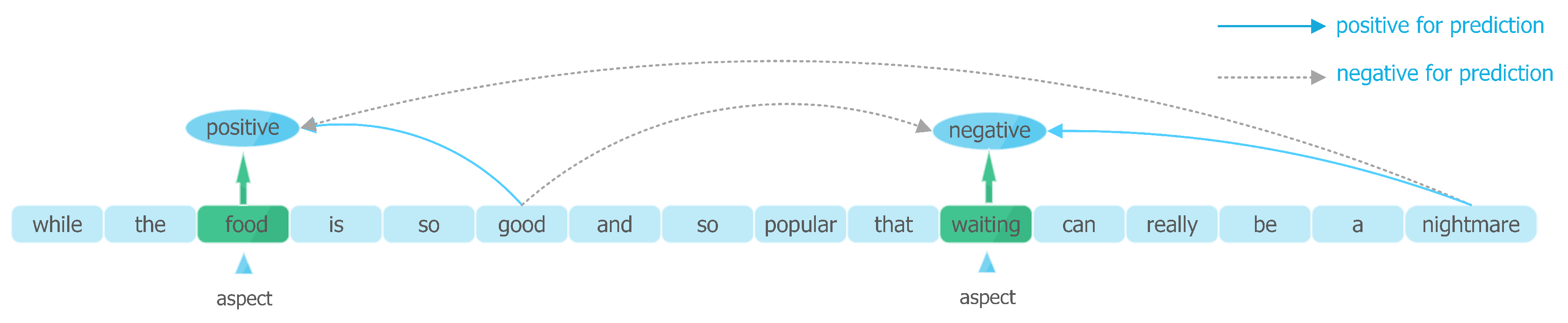
Aspect-based sentiment classification (ABSC) [1,2] is a fine-grained Natural Language Processing (NLP) task, and it is a significant branch of sentiment analysis [3,4,5,6]. Traditional sentiment analysis approaches [7,8,9,10] mainly focus on inferring sentence-level or document-level sentiment polarities (typically positive, negative, or neutral in triple-classification). However, the ABSC task, also known as aspect-based sentiment analysis (ABSA), differs from traditional sentiment analysis. It aims to predict independent sentiment polarities for targeted aspects within the same sentence or document. Aspect-based sentiment classification local contexts people make full use of the sentiment polarity, subjectivity and further information from targeted aspects. The ABSC datasets are composed of plenty of contexts and aspects. For example, reviews from customers usually comment on different aspects, and different aspects may deliver different sentiment polarities. Given sentences like “while the food is so good and so popular that waiting can really be a nightmare”. Definitely, the customer compliments the food but criticizes the service. Due to certain reasons, the restaurant makes the customer wait for a long while. Generally, traditional sentence-level or document-level sentiment polarity mining methods cannot precisely predict polarities for specific aspects as they do not consider the fine-grained polarities of different aspects.
Deep Neural Networks (DNNs), such as Recurrent Neural Networks (RNNs) and Convolutional Neural Networks (CNNs), are employed in NLP tasks in recent years, and those DNN-based models are proven to be efficient as well as an effective way to learn and deal with features of documents, sentences, words, and even tokens. Self-attention, which has been introduced in transformer [11] architecture, is a new attention mechanism compared to the traditional attention mechanism [12,13,14] to capture internal correlation of input representations. Experimental results have proved that self-attention performs much better than traditional DNN architectures in capturing features for Sequence to Sequence (Seq2Seq) tasks. BERT [15] is a pretrained linguistic model that can be adapted to many NLP tasks; it attained state-of-the-art performance on 11 NLP tasks. LCF design incorporates pretrained BERT model with LCF design as shared layers, and it outperforms state-of-the-art performance among three ABSC datasets.
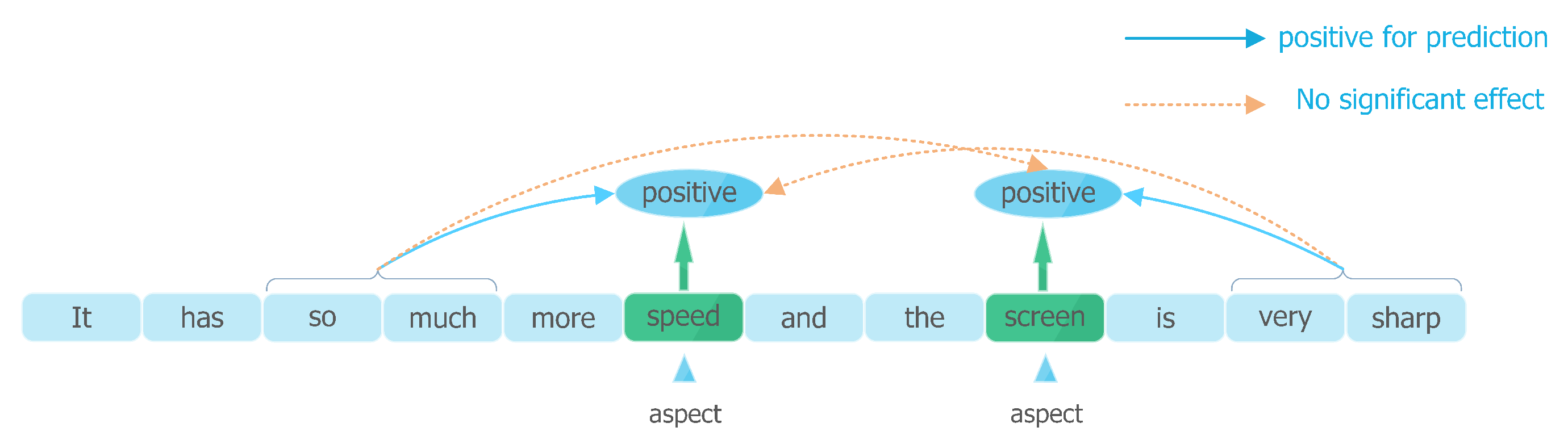
Almost none of the previous studies took the significant emotional information contained in aspect’s local context into considerations. Indeed, traditional DNN-based methods only focus on analyzing the correlations of the global context and sentiment polarities before identifying the sentiment polarity of targeted aspect based on global context features. However, LCF design notices that sentiment polarity of an aspect is more relevant to the context words near to itself. Moreover, the context words far from the aspect probably tend to cause negative influence to precisely predict the polarity of specific aspect (see Figure 1 and Figure 2). For example, semantics, adjectives, adverbs, and other subjective presentations are usually placed to the aspects which they modify. Further, they are more semantic-relative to the aspect which they are closed to. In that case, Semantic-Relative Distance (SRD) (see Section 3.2) is proposed to determine if a contextual word is the local context of a specific aspect. CDM and CDW layers concentrate on local context with the help of SRD. Based on Multi-Head Self-Attention (MHSA) different from previous methods, LCF design models learn the features from the sequence-level global context, but also from local context words associated with a specific aspect. LCF design compute local context features according to SRD.
The main contributions of this paper are as follows:
- This paper proposes LCF design models, which utilize self-attention to capture local context features and global context features concurrently. LCF design models combine local context features and global context features to infer sentiment polarity of targeted aspect.
- We introduce SRD to evaluate the dependency between contextual words and aspects. SRD is significant for figuring out local context, and features of contextual words in SRD threshold will be preserved and focused.
- This paper implements CDM and CDW layer to enforce LCF design models to pay more attention to local context words of specific aspect. The CDM layer focuses on local context by masking output representations of less-semantic-relative contextual words. The CDW layer weakens the features of less-semantic-relative contextual words according to SRD.
- Experiments conducted for ablated LCF design models to evaluate the significance and effectiveness of LCF design architectures. Besides, extra experiments are also carried out to evaluate the effectiveness of different SRD thresholds.
2. Related Works
In recent years, a variety of methods have been introduced to deal with the ABSC task, including traditional machine learning methods and neural network methods. In this section, we will introduce the related work of aspect-level sentiment classification, including traditional machine learning methods and deep learning methods.
2.1. Traditional Machine Learning Methods
In general, traditional machine learning approaches [16,17] for the ABSC task are primarily based on feature engineering. This also means that a lot of time is spent collecting and analyzing data, then designing features based on the characteristics of the dataset and obtaining enough language resources to construct lexicons. Supported Vector Machine (SVM) [16] is a traditional machine learning method and is applied to solve aspect-level sentiment classification and achieve a considerable performance. However, consistent with most traditional machine learning methods, this method is very burdensome and inefficient to design features manually. In addition, when the dataset changes, the performance of the method is greatly affected. Therefore, the methods based on traditional machine learning have poor generality and are difficult to apply to a variety of datasets.
2.2. Deep Learning-Based Methods
Recent works are growing to combine with Neural Networks (NN) because NN-based methods equipping with the remarkable ability to capturing original features, which can map the features into continuous and low-dimensional vectors without feature engineering.
Word embedding [18] is the basis of most DNN-based methods, which represents natural language as continuous low-dimensional vectors and learns interfeatures of natural language by operating the vectors. Word2vec [19], PV [20], and GloVe [21] are the pretrained word embeddings. These pretraining word embeddings are all trained on a large amount of text corpus (a typical source of text data is the corpus of Wikipedia). DNN-based methods map each word into a vector and learning the vector representations of the words according to the word embeddings. Pretrained word embedding can not only accurately reflect the relationship between words, but also significantly improve the performance of DNN-based models.
Attention mechanism [22], which is applied in plenty of DNN-based models, improves the performance for most NN-based models. The attention mechanism takes advantage of the semantic correlation of context and aspect to calculate the attention weights for context words, enforcing DNN-based models to obtain fine-grained aspect-level sentiment polarity. DNNs become very popular and play a more important role in NLP tasks than traditional machine learning methods, especially RNNs and CNNs. However, neural networks usually apply backpropagation to update the weight of hidden layer of the network. When the network is deep, the gradient vanishing problem occurs, which causes the weight of the hidden layer close to the input layer to be updated very slowly. It is a long-standing issue in the neural network. Long Short-Term Memory (LSTM) [23] is an advanced RNN network that can alleviate the gradient vanishing problem. However, like most RNNs, LSTMs can hardly be trained in parallel and they tend to be time-consuming since they are time-serial neural networks. Moreover, LSTMs are not suitable to process the interactive correlation of context and aspect, which would cause a tremendous loss of aspect information. TD-LSTM is proposed by the authors of [24], an RNN-based architecture that can obtain context features from both left and right sides. ATAE-LSTM [12] applies an attention mechanism and assembles the representations of aspect and context by concatenating them. ATAE-LSTM enables aspects to participate in computing attention weights.
Previous works regard targeted aspects such as independent and auxiliary information. However, experimental results show that these methods have limited effectiveness improvement for ABSC task. IAN, which is proposed by the authors of [13], generates the representations of context and aspect. IAN applies attention mechanism to interactively learn the features of context and targeted aspect, which enhances the interactively-learning process of aspect and context. IAN first proposed the interactive learning of context and aspect words. RAM [25] adopts multilayer architecture based on bidirectional LSTMs, and each layer contains attention-based aggregation of token features and Gated Recurrent Units (GRU [26]) to learn the sentence features. For the first time, RAM noticed varying degrees of contribution to learning from different contexts. MGAN [27] introduces a novel multigrained attention network, which uses a fine-grained attention mechanism to capture the word-level interaction between aspect and context.
A notable trend is that the pretrained model has gradually become a research hotspot of the ABSC task. The main characteristic of the pretraining model is to train a highly universal Language Model (LM) based on massive corpus resources. The pretraining model can be applied to a large number of NLP tasks and significantly improve the performance of each task. ELMo [28] and GPT [29], which are based on LSTM and transformer, respectively, are pretrained language models designed to improve the performance of many NLP tasks. In addition, BERT-PT [30] explores a novel post-training approach for question answering (QA) task on the pretrained BERT language model, which can be adapted to aspect-level sentiment classification task. BERT-SPC is the BERT text pair classification model, which is adapted to finish the ABSC task by the authors of [31]. BERT-SPC prepares the input sequence by appending aspect to contexts, regarding context and aspect as two segments.
3. Methodology
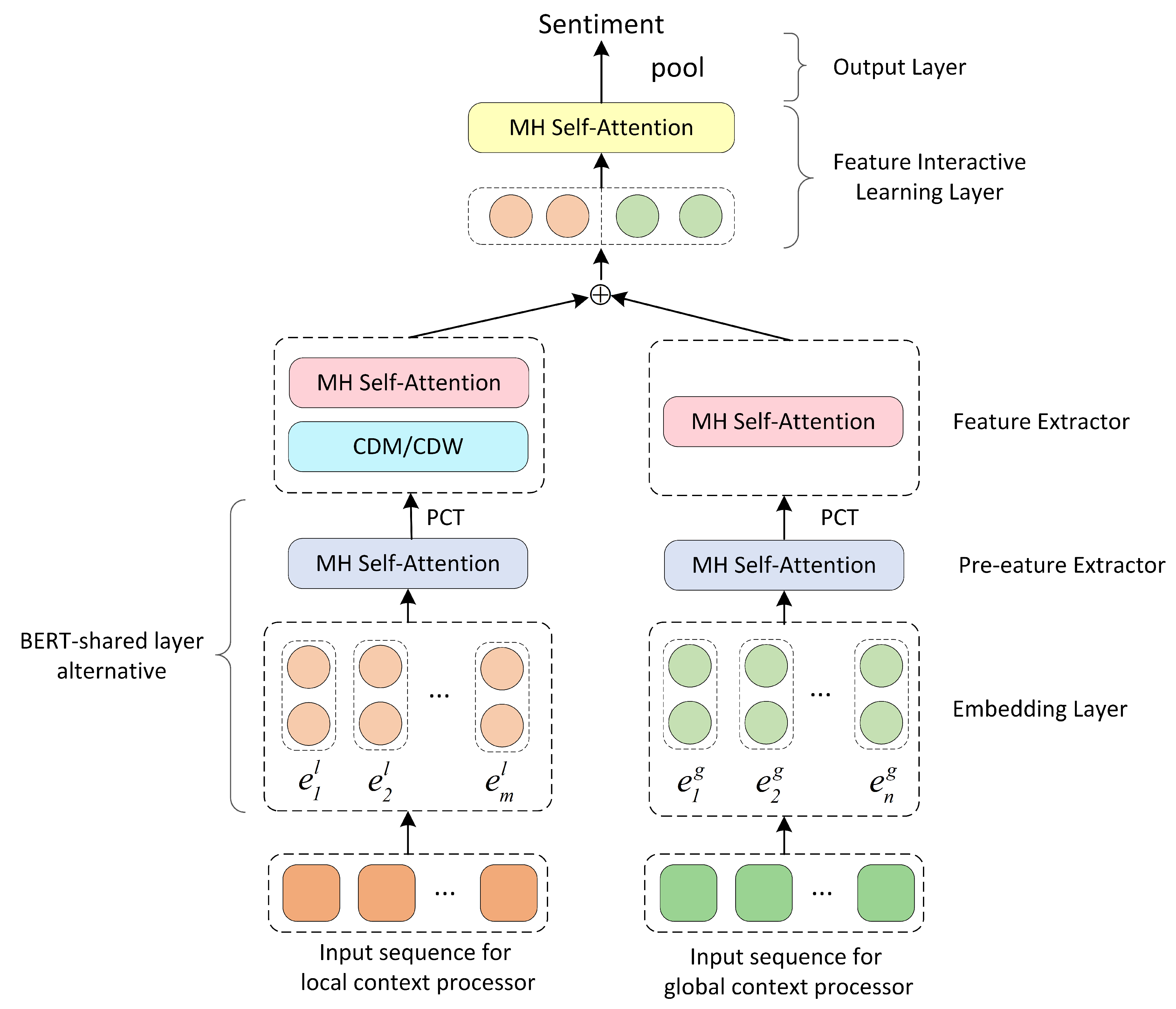
In this paper, an LCF design is implemented with two embedding layers. In the LCF baseline model, GloVe [21] word embedding is adopted as the embedding layer to accelerate the learning process and attain better performance. The LCF baseline model is called as LCF-GloVe. As for another architecture of LCF design, we substitute GloVe embedding layer and feature extractor layer with BERT shared layer, the LCF-BERT model. A shortcut of the LCF design overall architecture is shown in Figure 3.
Apart from the embedding layer, the LCF-GloVe is slightly different from LCF-BERT, as LCF-GloVe mainly relies on Multi-Head Self-Attention instead of BERT-shared layer to learn local context features and global context features respectively. Moreover, the input sequence for LCF-GloVe could be slightly different between local context processor and global context processor. The LCF-GloVe requires the input of the whole context sequence accompanied with aspect.
The LCF-BERT model attains a dramatically high performance compared to current state-of-the-art models. Motivated by the BERT-SPC model, the input of global context processor of LCF-BERT model adopts the context input sequence consistent with BERT-SPC [31]. In the local context sequence, aspects will be preserved, because the LCF design can learn the interactive relation between context and aspect, which strengthens the capability of LCF design to determine the deep correlation of context and aspect.
3.1. Task Definition
For aspect-based sentiment classification, the prepared input sequences for model generally consist of context sequence and aspect sequence, which enables the model to learn the correlation of context and aspect. Suppose that is an input context sequence with aspect included, the sequence contains words including targeted aspects. is a targeted aspect sequence. Meanwhile, is a subsequence from , which is composed of words.
3.2. Semantic-Relative Distance
The majority of previous works divide the input sequence into aspect sequence and context sequence and modeling for their interrelation. However, this paper proposes a new idea: apart from the global context, the local context of targeted aspects contains more significant information. Therefore, one of the most important things is how to determine whether a contextual word belongs to the local context of a specific aspect or not. In order to solve this problem, this paper proposes SRD, which aims at assisting models to capture local contexts.
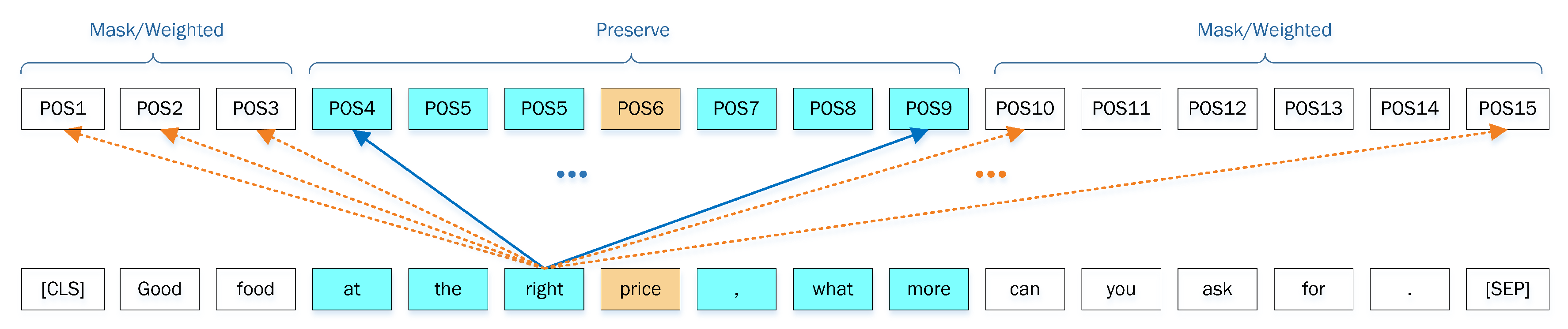
LCF design counts tokens between each contextual token towards specific aspect as the SRD of all token-aspect pairs (see Figure 4 and Figure 5). For example, if the SRD threshold is set to be 5, each context word whose SRD towards an aspect less than the threshold will be regarded as the local context. Take the same review example as mentioned above, “while the food is so good and so popular that waiting can really be a nightmare”, for the aspect of food, its local contexts words are while the [asp] is so good and so”, [asp] represents the aspect sequence, which may be composed of several words or tokens. In this local context sequence, [asp] means “food”. LCF calculates the SRD as follows.
where i and are the position of the contextual word and central position of aspect, respectively. m is the sequence length of the aspect. represents for the SRD between the i-th contextual token and specific aspect.
LCF design models completely preserve original features of aspects and its local context. Through the experiments and analysis, it is concluded that SRD is of great importance for LCF models.
3.3. Embedding Layer
The embedding layer is the basic layer of LCF design models. Each word and token will be mapped to a vector space through embedding layers. In LCF design, GloVe word embedding and the BERT-shared layer are alternatives for the embedding layer.
3.3.1. GloVe Word Embedding
LCF-GloVe adopts the pretrained GloVe word embedding to accelerate the learning process and retain better performance. Suppose is the GloVe embedding, is the dimension of embedding vector, and is the size of vocabulary. Then, each contextual word will be embedded into a vector .
3.3.2. BERT-Shared Layer
The BERT-shared layer is a pretrained Seq2Seq model for language understanding, and it can be regarded as the embedding layer. In order to achieve better performance, the fine-tuning learning process is necessary and indispensable. LCF-BERT adopts two independent BERT-shared layers to model local context sequence features and global context features, respectively. For the input of local context and global context representations and , respectively, we have
and are the output representations of local context and global context processor, respectively. and are the corresponding BERT-shared layer modeling for local context and global context, respectively.
3.4. Pre-Feature Extractor
The BERT-shared layer is powerful enough to capture context features. However, LCF-GloVe eschews the BERT-shared layer and adopts GloVe word embedding as the embedding layer. In order to improve the capability of LCF design for learning semantic features, we design the Pre-Feature Extractor (PFE). PFE is composed of MHSA layer and Position-wise Convolution Transformation [31] (PCT) layer.
3.4.1. Multi-Head Self-Attention
Based on a self-attention mechanism, Multi-Head Self-Attention performs multiple attention functions to compute attention scores for each contextual word. For the self-attention function, Scaled Dot Product Attention (SDA) is recommended as the identical attention function, for it is faster and more efficient in the calculation.
Suppose is the input representation embedded through embedding layer. The definition of SDA is as follows,
and V are obtained by multiplying the output representation of the upper layer’s hidden states by their respective weight matrix , , . And these weight matrices are trainable during learning process, Dimensions are equal to , is the dimension of hidden layer. The attention representations learned by each head will be concatenated and transformed by multiplying a vector . In LCF design, the number of attention heads, h, is set to be 12. Suppose is the representation learned by each attention head, then we have
where “;” denotes vector concatenation . Additionally, a tanh activation function is deployed for MHSA encoder to enhance learning capability of the representations.
3.4.2. Position-Wise Convolution Transformation
Position-Wise Convolution Transformation (PCT) is adapted to the LCF design as a trick. According to experimental results and sufficient analysis, it can slightly improve the performance of LCF design on laptop dataset. The input representations for PCT layer is the output representation of MHSA encoder. The definition of PCT is as follows
denotes the activate function of ReLU; and are the traniable weights vectors of the two convolutional kernels, respectively; and and are the biases vectors of the two convolutional kernels.
Then, the output representations of PFE layer generated are as follows
Word embeddings of the local context and global context, and , respectively, are learned by the MHSA encoder, giving out and . are the output representations of local context and global context processed by corresponding PFE layer. and denote the PCT layers that aim at improving the performance on laptop dataset.
3.5. Feature Extractor
The LCF design deploys a Feature Extractor (FE) layer to learn features of the local context and global context. If only taking the local context into consideration, it would inevitably ignore the features of less-semantic-relative context words. In order to fully retain the features contained in the global context and learn the correlation between global context and aspect, LCF models take the global context features as a supplement to enhance LCF design.
The local context feature extractor is much different from global context feature extractor, for it contains a local context focus layer, while the global context feature extractor is only equipped with an MHSA encoder.
3.5.1. Local Context Focused Layer
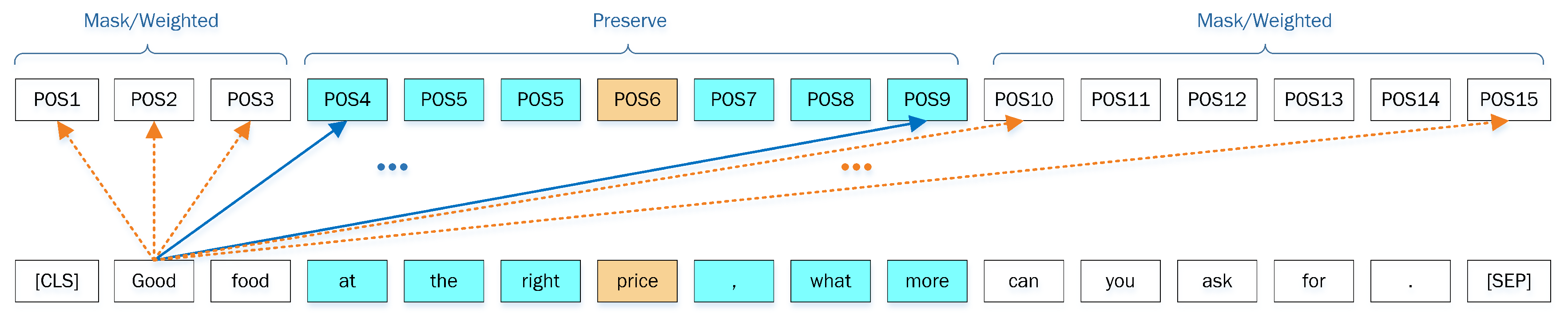
Figure 4 and Figure 5 are the abstracts of the local context focus mechanisms. Each token in the bottom of the figure comes from the input sequence, and the position (POS) in the top of the figure represents the output position of the corresponding token. The self-attention mechanism enables all tokens to calculate the attention scores with other tokens in parallel and react in the corresponding output position. To simplify the picture, we select two tokens to show their context-focused process with other tokens. After calculating the output of all tokens from the attention layer, the output features on each output position above the SRD threshold will be masked or weakened, while the output features of local context words will be completely retained.
The input sequences of the LCF design are mainly based on the global context. LCF design models focus on local context by adopting local context focus layer. This paper implements two architectures to focus on local contexts CDM and CDW (see Figure 4 and Figure 5). We apply MHSA encoders instead of CNN or RNN architecture due to the following considerations. On the one hand, MHSA is more powerful to capture context features. On the other hand, self-attention calculates correlation attention scores for every contextual word, and, according to the self-attention definition, the word itself holds the highest score on its corresponding output position generally.
Table 1 is the algorithm flow of CDM and CDW mechanism. LCF design layers preserve the features of semantic-relative contextual words while masking or weighing the features of less-semantic-relative contextual words. So the less-semantic-relative context can participate in the encoding process and their passive influence are alleviated.
3.5.2. Dynamic Mask for Context Features
CDM layer masks the less-semantic-relative context features learned by PFE or BERT-shared layers. Although it is easy to mask the less-semantic-relative contextual words in the input sequence, it also will absolutely discard the features of less-semantic-relative contextual word. With the CDM layer deployed, only the features of the less-semantic-relative context itself on the corresponding output position will be masked. The correlative representations between less-semantic-relative context word and aspect are reserved on corresponding output positions.
All masked features will be set to zero vectors. Another MHSA encoder is deployed to learn the masked context features. In this term, LCF design can alleviate the influence of less-semantic-relative contexts, but reserve the correlation between each contextual word and aspect. Suppose is the output representation of local context feature extractor, CDM focuses on the local context by constructing the mask vectors for each less-semantic-relative context word, so we get the mask matrices M.
where is the SRD threshold. M is the mask matrices for the representation of input sequences and n is the length of input sequence including aspect. is the ones vector and is the zeros vectors. is the output of CDM layer. “.” denotes the dot product operation of the vectors.
3.5.3. Dynamic Weighted for Context Features
In addition to CDM layer, another architecture is implemented to focus on local context words, the Context features Dynamic Weighted (CDW) layer. While features of a semantic-relative contextual word will be absolutely preserved, less-semantic-relative context features will be weighted decay. In this design, features of the contextual word that is far from the targeted aspect will be reduced according to their SRD. CDW weights the features by constructing the weighted vector for each less-semantic-relative context word, here is the formula to get mask matrices M for an input sequence:
where is the SRD between the i-th contextual token and a specific aspect. n is the length of the input sequence. is the SRD threshold. is the output of CDW layer. “.” denotes the vector dot product operation.
The output representation of local context FE can be attained based on the output of CDW or CDM.
For CDM layers:
For CDW layers:
Both the output representations of CDM and CDW layer are denoted as , and they are alternative and independent.
3.5.4. Global Context Features Extractor
In global context FE, the output of the features learned by MHSA encoder is as follows
where is the representation learned by global context PFE layer.
3.6. Feature Interactive Learning Layer
The Feature Interactive Leaning (FIL) layer is deployed to interactively learn the features of the global context. FIL first concatenates the representations of and , then projects them into and applies an MHSA encoding operation.
and are the weights and bias vector of the dense layer, respectively; an MHSA encoder will encode the , then output the interactively learned features .
3.7. Output Layer
In the output layer, the representation learned by feature interactive learning layer is pooled by extracting the hidden states on the corresponding position of the first token. Finally, a Softmax layer is applied to predict the sentiment polarity.
where C is the number of classes and Y is the sentiment polarity predicted by LCF design model.
3.8. Model Training
The LCF design includes LCF-GloVe and LCF-BERT; most of the architectures are identical except the embedding layer and PFE layer. For the LCF-GloVe model, the input sequence for local context processor and global context processor is the whole review, e.g., “while the food is so good and so popular that waiting can really be a nightmare”. For the LCF-BERT model, the input sequence for the local context processor will be refactored to “[CLS]” + “while the food is so good, it is so popular that waiting can really be a nightmare.” + “[SEP]”, and the input sequence for global context processor are the same as the input sequence of BERT-SPC, e.g., “[CLS]” + “while the food is so good and so popular that waiting can really be a nightmare.” + “[SEP]” + [asp] + “[SEP]”.
Similar to LCF-GloVe, the MHSA encoders of LCF-BERT are independent. Moreover, the BERT-shared layers for local context processor and global context processor are independent.
LCF design applies the cross-entropy loss function for LCF design with regularization, and we define the loss function as follows.
where C is the number of classes, is the regularization parameter, and is the parameter set of the LCF model.
4. Experiments
4.1. Datasets and Hyperparameters
Experiments are conducted on three ABSC benchmark datasets, a review dataset of laptop, a review dataset of restaurants from SemEval-2014 [1] and a common ACL 14 twitter social dataset introduced by [32]. According to the experimental results, the performance of the LCF design on the datasets of three topics (restaurant reviews, laptop reviews, and tweets) has been significantly improved, which indicates that the LCF design does not rely on specific datasets or corpora and it is applicable to most topics of datasets, which is due to the original characteristics of natural language (Suppose people comment on multiple aspects in a review, then, the context word used to judge an aspect is likely to be near the aspect generally, and not far from the aspect word to be commented on.). These datasets are adopted by most of the proposed models and are the most popular datasets of ABSC task, and a large number of experiments have been carried out on these datasets for comparison. These datasets provide labeled aspects such as the sentiment polarities of the aspects. All aspects of the above datasets are labeled in three categories of sentiment polarities: positive, neutral, and negative. In the experiments, these datasets are original and under no refactor, and no conflicting label is removed. In that case, it can provide a better estimate of the real performance of the model. Table 2 demonstrates the details of three datasets (Generally, both LCF-GloVe and LCF-BERT converge within three epochs during the training process.).
To evaluate the precise difference of performance, the hyperparameters are kept consistent for LCF-GloVe model and LCF-BERT model except for learning rate, because BERT-shared layer requires very small learning rate during fine-tuning process [15]. For LCF-GloVe, the learning rate is set to . The hidden dimension and embedding dimension, , and , are set to 300. For LCF-BERT, the learning rate is set to . The hidden dimension and embedding dimension are set to 768 in LCF-BERT. For both LCF design models, dropout rates are set to 0, regularization is set to , and the batch size is set to 16. In addition, LCF models utilize the Adam optimizer [33].
All hyperparameters in this paper have been supported by a large number of comparative experiments. Among them, most of the hyperparameters follow the common hyperparameter settings of this task, such as the word embedding dimension and learning rate of LCF-GloVe model. We tried different thresholds to find the optimal threshold for each dataset (see Table 5). The fine-tuning process of BERT is very sensitive to the learning rate. Only a small learning rate can maximize Bert’s performance, which has been illustrated in the original paper of BERT. Through the experiments, we observed that when batch size was large, the instability of regularization between layers would reduce the performance of the model, so the optimal batch size of 16 was adopted. Large dropout will prolong the convergence rate of the LCF-BERT model, and experimental results show that they have no obvious influence on LCF design. Therefore, after comprehensive consideration, dropout of the model is designed to be 0. For both LCF design models, accuracy and Macro-F1 score are adopted to evaluate the performance of LCF designs. Because experimental results tend to fluctuate, this paper chooses the best experimental results to make comparisons.
4.2. Comparison Models
We evaluate the performance of the LCF design on three datasets and compared with multiple baseline models. The results reveal that LCF design can greatly improve the state-of-the-art performance on three data sets, especially the LCF-BERT model. The LCF design models are compared with the following models.
TD-LSTM [24] TD-LSTM divides the input sequences into left context and right context towards a specific aspect. Moreover, two LSTM networks are adopted to modeling the left context sequence and right context sequence with targeted aspect respectively. Both left and right target-dependent representation are processed by corresponding LSTM networks and are concatenated as a unity to predict sentiment polarity of targeted aspect.
ATAE-LSTM [12] ATAE-LSTM implements an attention mechanism to assist mode to focus on more relative context to targeted aspects. Meanwhile, ATAE-LSTM appends aspect embeddings with each word embedding, which strengthens model by learning the hidden relation between context and aspect.
IAN [13] IAN generates representations of targeted aspects and context by two LSTM networks, respectively. IAN learns the representations of targeted aspect and context interactively. Interactive attention mechanism brings a considerable performance improvement.
RAM [25] RAM improves the MemNet [34] by representing memory with BiLSTM neural networks. Meanwhile, a gated recurrent unit network was introduced to learn the features processed multiple attention mechanism.
BERT-PT [30] BERT-PT explores a novel post-training approach on the BERT pretrained model to improve the performance of fine-tuning of BERT for RRC task. Additionally, the BERT-PT method can be adapted to ABSC task.
BERT-SPC [31] BERT-SPC is the Sentence Pair Classification task of pretrained BERT model. BERT-SPC for ABSC task constructs the input sequence as “[CLS]” + global context + “[SEP]” + [asp] + “[SEP]”.
4.3. Overall Performance Comparison
Table 3 demonstrates the main experimental results. According to experimental results, LCF design models perform well among three benchmark datasets, especially on the laptop dataset and restaurant dataset. The LCF-BERT model attains impressive improvement for outperforming state-of-the-art performance. Compared to the BERT-PT model, it improves the performance by 3–4% in the laptop dataset and 2–3% in the restaurant dataset. However, compared to MGAN, the LCF-GloVe model achieves a limited performance in the twitter dataset. After further analysis, it is found that the twitter dataset is a social dataset, and there are lots of misspelled words and unknown tokens. Moreover, it is found that plenty of tweets are composed of informal linguistic expressions as well as grammatically incorrect expressions, causing difficulty when extracting high-quality semantic representations. Generally, the CDM layer works well in the LCF-GloVe model. Probably the local context plays a more important role in feature extraction since MHSA has a limited power to extract global context features. In addition, the CDW layer achieves remarkable performance in the LCF-BERT model, because the BERT-shared layer is more powerful when extracting and learning context features, including the local context and global context.
The experiments show that the local context focus mechanism is applicable to the self-attention and can achieve excellent results. However, while applied into many kinds of DNNs, the performance of local context focus layer in RNNs (LSTM and GRU) is not optimal. At the same time, local context focus mechanism provides a new approach to fine-grained aspect-level sentiment classification, which significantly avoids the influence of distant context in the mechanism of self-attention, and achieves a state-of-art effect on the three commonly used ABSC datasets. Once applied to different ABSC models, the local context focus mechanism will bring significant performance improvement to models.
4.4. Analysis of LCF design Models
Both LCF-GloVe and LCF-BERT are equipped with CDM and CDW local context focus layers. The experimental results indicate that LCF designs are very effective. In addition, CDM and CDW are feature-level operations (see Figure 4 and Figure 5), instead of directly operating the input tokens. Owing to the MHSA encoder, CDM and CDW can involve less-semantic-relative tokens in the learning process, then retain their semantic features towards semantic-relative tokens. However, CDM and CDW mitigate the features of less-semantic-relative tokens on corresponding output positions, which enable LCF design models to focus on the local context. Another significant thing is that LCF design also learns the features of the global context. Owing to the interactive learning of local context and global context that LCF design achieves such remarkable results (see Table 4).
4.5. Ablations and Variations of LCF Design
In order to analyze the importance of each LCF design layer, ablation and variation experiments are designed for LCF-GloVe as well as LCF-BERT. Experimental results are listed in Table 4.
4.5.1. Ablate Pre-Feature Extractor Layer
For LCF-GloVe, the pre-feature extractor is deployed between the embedding layer and feature extractor in LCF-Glove model, since it can enhance the performance of GloVe embedding layer. The pre-feature extractor consists of MHSA and PCT layer. We ablate the pre-feature extractor layer to examine the performance of LCF without it.
LCF-GloVe (CDM/CDW) without PFE layers performs better than baseline models on twitter dataset, while its performance on laptop dataset descends obviously. On the restaurant dataset, LCF-GloVe (CDM/CDW) almost achieve an equal performance compared to baseline models. PFE layers are deployed to learn the features embedded by GloVe embedding layer. The MHSA encoder is pretty different from the traditional encoder as it contains positional embedding. In order to adapt the GloVe embedding representation to MHSA encoder, PFE layers are designed to preprocess the embedding representations. Table 4 indicates that PFE layers are very significant for LCF-GloVe (CDM/CDW) on laptop dataset.
4.5.2. Ablate CDM/CDW Layer
The CDM layer and CDW layer are core architecture for the LCF design. We ablate the CDM and CDW layer and utilize the global context features to predict sentiment polarities for targeted aspects.
For the LCF-GloVe ablation experiment, LCF-GloVe with “only Glo” means that only global context features are captured and learned, and no CDM or CDW layer is deployed in this ablation. This ablation achieves inferior performance among three datasets, which indicates that CDM layer and CDW layer are very effective for LCF design models. LCF-GloVe with “only CDM” performs moderate performance among three datasets, and its performance on the restaurant dataset is equal to the baseline model. Moreover, LCF-GloVe with “only CDW” attains worse performance on three datasets compared to LCF-GloVe with “only Glo”.
For the LCF-BERT ablation experiment, LCF-BERT with “only Glo” attains a considerable performance compared to LCF-BERT with “only CDM” and LCF-BERT with “only CDW”. However, there is still a gap of performance on three datasets between both three ablations and their baseline model.
4.5.3. Ablate Feature Interactive Leaning Layer
Feature Interactive Learning (FIL) layer aims at assembling features and interactively learns the correlation between local context and global context. Concatenation and pooling can substitute the FIL layer, but there is no interactive learning process.
For LCF-GloVe-CDM without FIL layer, performance on restaurant and twitter datasets are close to the baseline models, and performance on laptop dataset is slightly poor. LCF-GloVe-CDW without FIL layer performs better on restaurant dataset, but achieves inferior performance on other two datasets.
For LCF-BERT (CDM/CDW) without FIL, they attain inferior performance on three datasets, which means FIL layer is of great significance for LCF design.
4.5.4. LCF-Ablations Analysis
According to Table 4, the performance of LCF ablations was significantly reduced. Compared to baseline models, the LCF-GloVe ablations of PFE layer achieve limited performance on three datasets, especially on laptop dataset. Both LCF-GloVe and LCF-BERT attain inferior performance when only the global context or local context is taken into consideration since LCF will lose significant features. We design a FIL layer to interactively learn the features of the global context and local context. Without the FIL layer, performance on three datasets drops obviously. The experiments reveal that, for both LCF-GloVe and LCF-BERT, all the components work fine and bring a huge improvement among three datasets. For LCF-BERT, if only the local context is taken as input, the performance decreases by 2–3%. Experimental results show that each component of LCF design is indispensable and effective.
4.5.5. LCF-GloVe Variations about SRD Threshold
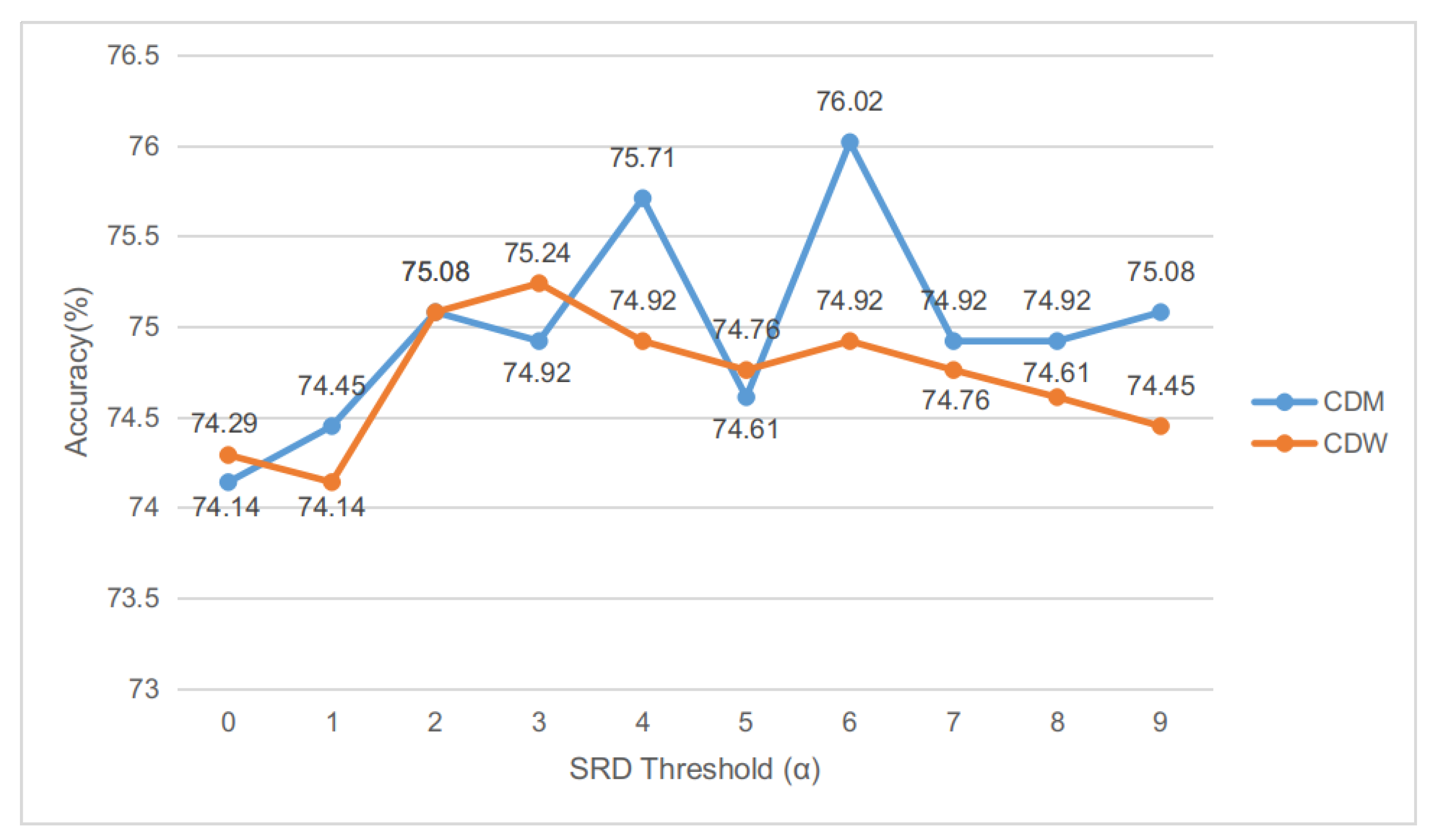
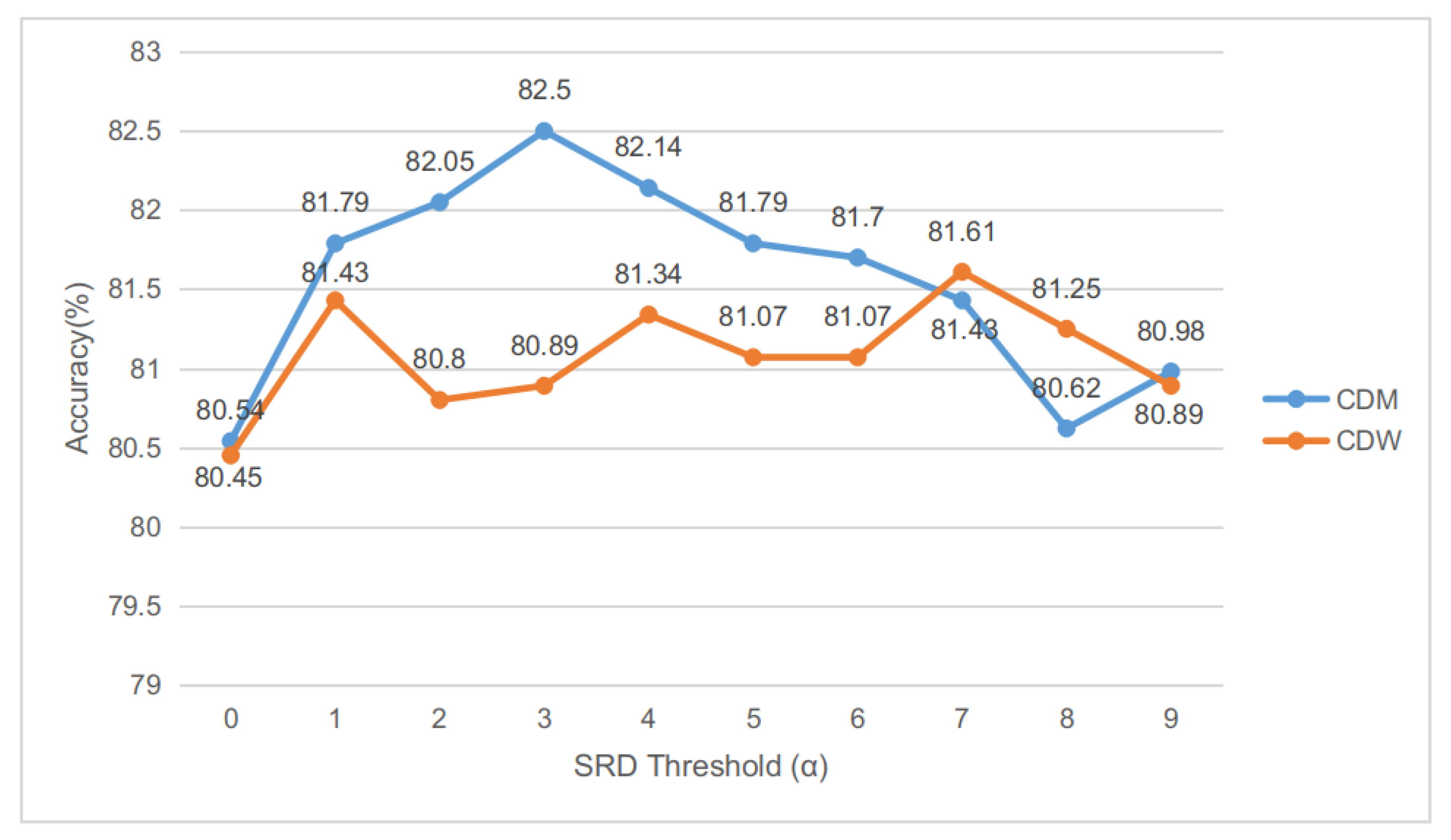
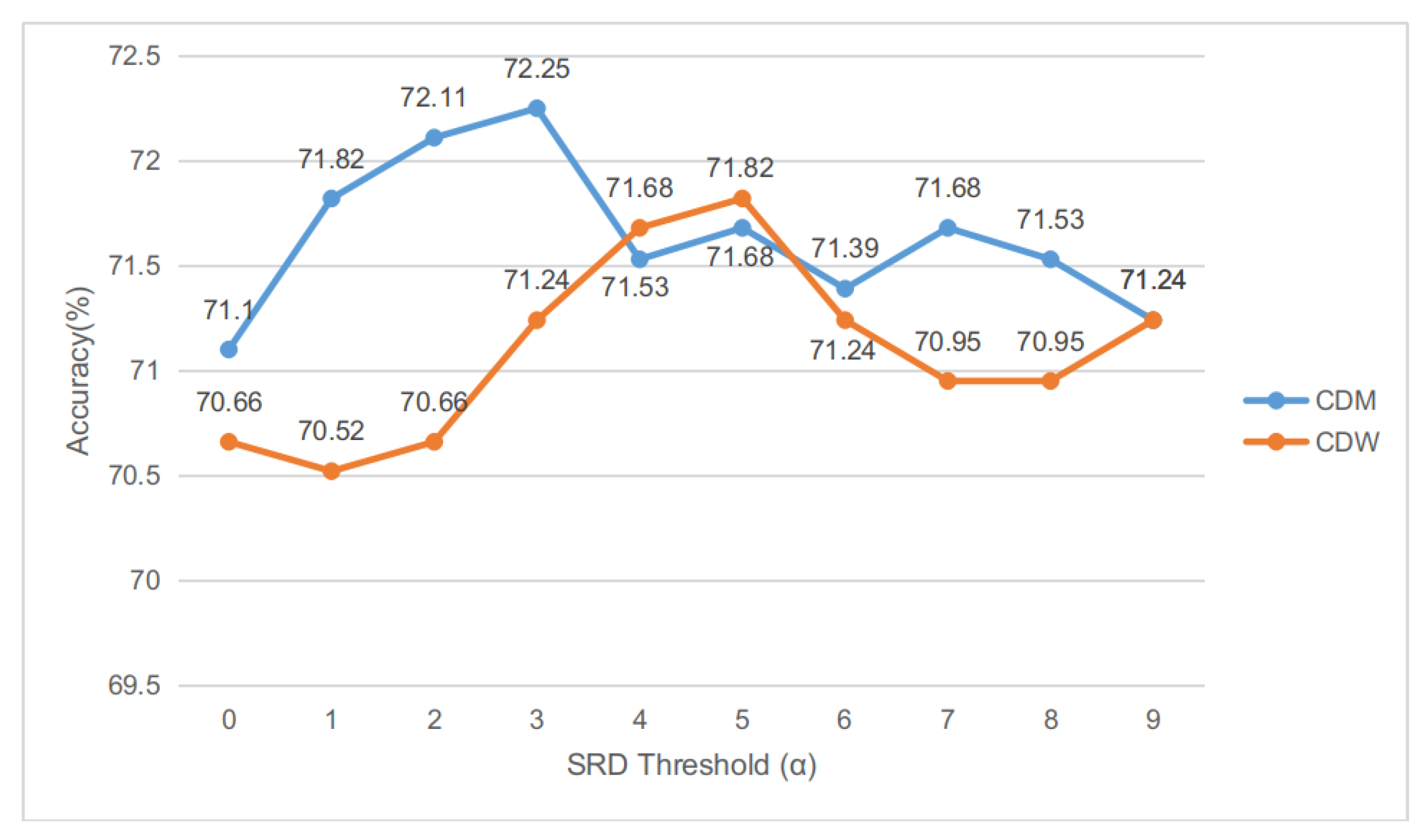
For LCF-BERT, it is hard to evaluate sufficient SRD variation experiments since the BERT-shared layer is not space-efficient (the number of parameters of LCF-BERT is approximately ), while the number of parameters of LCF-GloVe is approximately . In that case, the is set to be 3 for CDW and CDM design on three datasets.
In order to find superior for different LCF design and datasets, a series of experiments about SRD threshold on LCF-GloVe are conducted to evaluate the best for different situations. In the comparison experiments, the SRD of the corresponding model and dataset ranges from 0 to 9, and the local context will be equal to the aspect itself if the SRD threshold () is 0. In these comparison experiments, all the parameters and hyperparameters are consistent with LCF-GloVe or LCF-BERT except SRD thresholds. Due to the fluctuation of experimental results, many experiments have been carried out to find the best results for comparison.
Actually, the SRD threshold is not very sensitive for LCF-GloVe-CDW design, and the performances on three datasets fluctuates slightly (Our extra experiments prove that CDW and CDM designs perform well and stably on LCF-BERT.) (see Figure 6, Figure 7 and Figure 8). The LCF-GloVe CDM design is stable among the three datasets, and the superior for all situations can easily be found out (see Table 5).
5. Conclusion and Future Works
This paper proposes a new view: local context words of specific aspects are more relevant to the aspect. LCF designs focus on the local context and learn global context representations in parallel. This paper introduces SRD to assist locate the local context of each aspect. With the local context of targeted aspects supervised, LCF models work more stably and precisely in aspect-level sentiment classification. Both GloVe word embeddings and BERT-shared layer are utilized to improve the performance of LCF designs. With CDM and CDW applied, LCF-BERT outperforms state-of-the-art performance in three ABSC datasets. In future, the SRD calculation can be further improved by considering extra auxiliary information. Besides, the transferability of CDM and CDW designs will be evaluated whether they can improve the performance of the models those based on self-attention.
6. Case Analysis
In this section, we pick two samples from the laptop dataset and restaurant dataset for case analysis. They are “I how the black roasted codfish, it was the best dish of the evening” and “Lots of extra space but the keyboard is ridiculously small”, and we label them as sample-1 and sample-2, respectively. Sample-1 only contains one aspect and sample-2 contains two aspects. The is set to 3 for both samples.
6.1. One-Aspect
The polarity of aspect “dish” is predicted by LCF-ablated models and Table 6 shows the predicted results. Figure 9 and Figure 10 are visualizations of CDM and CDW processes of aspect “dish” within sample-1.
Results in Table 6 show that local context focus mechanism work performs well on one-aspect samples. Almost no LCF-ablated models make error prediction.
6.2. Multi-Aspect
Accordingly, Figure 11 and Figure 12 are visualizations of CDM and CDW processes of sample-1, respectively. The polarity of the aspect “space” is predicted by LCF ablated models and Table 6 shows the predicted polarities. The sentiment classification of multi-aspect samples are more complex compared to one-aspect samples, since each aspect probably has different sentiment polarity. Moreover, it is important to alleviate the negative influence of less-semantic-relative context words during learning process.
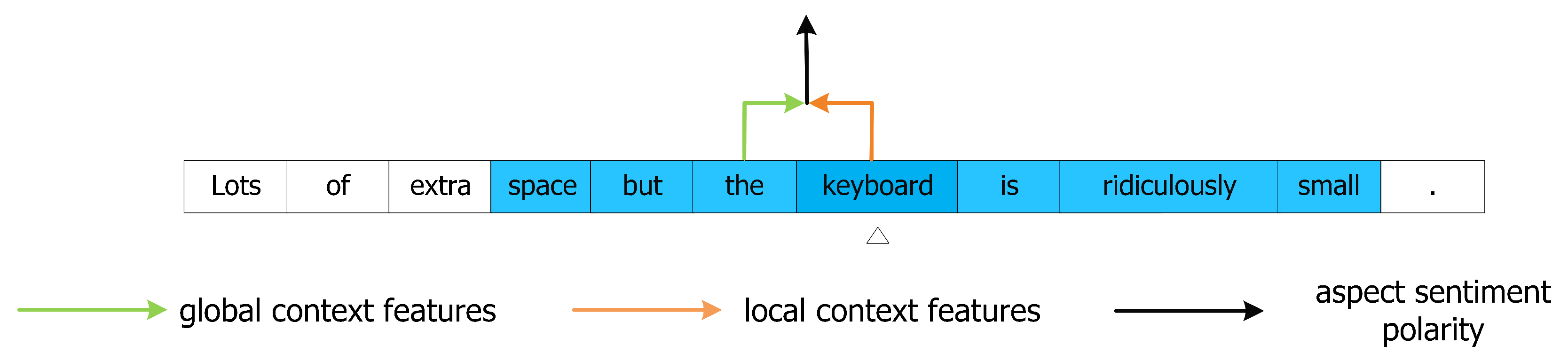
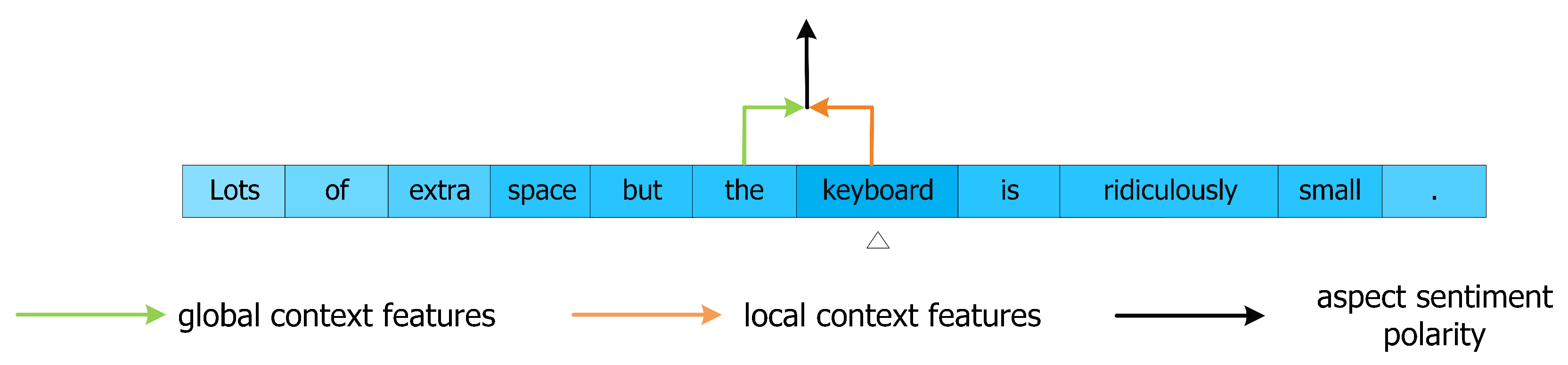
Consistently, Figure 11, Figure 12, Figure 13 and Figure 14 are visualizations of CDM and CDW processes of aspect “space” and “keyboard”, respectively, within sample-2. The polarities of these two aspects are predicted by LCF ablated models and Table 6 shows the predicted polarities.
Most of the LCF-ablated models generally give the correct predictions for aspect “space” and “keyboard”. Table 6 shows that the predictions of LCF-BERT are more accurate and reasonable than that of LCF-GloVe.
Equipped with the local context focus mechanism, LCF design models can better predict the sentiment polarities of aspects through the interactive learning of local context features and global context features, instead of making predictions merely relying on local context features or global context features.
While inhibiting the interference brought by distant context words to prediction, it can also retain the long-term dependencies between the aspect these words and the of local context words. Experiments show that this can significantly improve the prediction accuracy of the model, and refresh the best performance on the three commonly ABSC datasets.
Author Contributions
Conceptualization B.Z. and H.Y.; methodology, H.Y. and B.Z.; investigation B.Z.; formal analysis H.Y.; software, H.Y.; validation H.Y. and X.H.; writing, H.Y.; resources R.X. and X.H.; review, R.X., W.Z. and X.H.
Funding
This research was funded by National Natural Science Foundation of China, Multimodal Brain-Computer Interface and Its Application in Patients with Consciousness Disorder, Project approval number: 61876067.
Conflicts of Interest
The authors declare no conflict of interest.
References
- Maria Pontiki, D.G.; John Pavlopoulos, H.P.; Ion Androutsopoulos, S.M. Semeval-2014 task 4: SemEval-2014 Task 4: Aspect Based Sentiment Analysis. In Proceedings of the 8th International Workshop on Semantic Evaluation (SemEval 2014), Dublin, Ireland, 23–24 August 2014; pp. 27–35. [Google Scholar]
- Pontiki, M.; Galanis, D.; Papageorgiou, H.; Androutsopoulos, I.; Manandhar, S.; Mohammad, A.S.; Al-Ayyoub, M.; Zhao, Y.; Qin, B.; De Clercq, O.; et al. Semeval-2016 task 5: Aspect based sentiment analysis. In Proceedings of the 10th International Workshop on Semantic Evaluation (SemEval-2016), San Diego, CA, USA, 16–17 June 2016; pp. 19–30. [Google Scholar]
- Pang, B.; Lee, L. Opinion mining and sentiment analysis. Found. Trends® Inf. Retr. 2008, 2, 1–135. [Google Scholar] [CrossRef]
- Liu, B. Sentiment analysis and opinion mining. Synth. Lect. Hum. Lang. Technol. 2012, 5, 1–167. [Google Scholar] [CrossRef]
- Kim, H.; Jeong, Y.S. Sentiment Classification Using Convolutional Neural Networks. Appl. Sci. 2019, 9, 2347. [Google Scholar] [CrossRef]
- Agarwal, A.; Xie, B.; Vovsha, I.; Rambow, O.; Passonneau, R. Sentiment analysis of twitter data. In Proceedings of the Workshop on Language in Social Media (LSM 2011), Portland, OR, USA, 23 June 2011; pp. 30–38. [Google Scholar]
- Kanayama, H.; Nasukawa, T. Fully automatic lexicon expansion for domain-oriented sentiment analysis. In Proceedings of the 2006 Conference on Empirical Methods in Natural Language Processing. Association for Computational Linguistics, Sydney, Australia, 22–23 July 2006; pp. 355–363. [Google Scholar]
- McDonald, R.; Hannan, K.; Neylon, T.; Wells, M.; Reynar, J. Structured models for fine-to-coarse sentiment analysis. In Proceedings of the 45th Annual Meeting of the Association of Computational Linguistics, Prague, Czech Republic, 25–27 June 2007; pp. 432–439. [Google Scholar]
- Wilson, T.; Wiebe, J.; Hoffmann, P. Recognizing contextual polarity: An exploration of features for phrase-level sentiment analysis. Comput. Linguist. 2009, 35, 399–433. [Google Scholar] [CrossRef]
- Taboada, M.; Brooke, J.; Tofiloski, M.; Voll, K.; Stede, M. Lexicon-based methods for sentiment analysis. Comput. Linguist. 2011, 37, 267–307. [Google Scholar] [CrossRef]
- Vaswani, A.; Shazeer, N.; Parmar, N.; Uszkoreit, J.; Jones, L.; Gomez, A.N.; Kaiser, Ł.; Polosukhin, I. Attention is all you need. In Advances in Neural Information Processing Systems; Neural Information Processing Systems Foundation, Inc.: Long Beach, CA, USA, 2017; pp. 5998–6008. [Google Scholar]
- Wang, Y.; Huang, M.; Zhao, L. Attention-based LSTM for aspect-level sentiment classification. In Proceedings of the 2016 Conference on Empirical Methods in Natural Language Processing, Austin, TX, USA, 1–5 November 2016; pp. 606–615. [Google Scholar]
- Ma, D.; Li, S.; Zhang, X.; Wang, H. Interactive attention networks for aspect-level sentiment classification. In Proceedings of the 26th International Joint Conference on Artificial Intelligence, Melbourne, Australia, 19–25 August 2017; pp. 4068–4074. [Google Scholar]
- Li, X.; Bing, L.; Lam, W.; Shi, B. Transformation Networks for Target-Oriented Sentiment Classification. In Proceedings of the 56th Annual Meeting of the Association for Computational Linguistics (Volume 1: Long Papers), Melbourne, Australia, 15–20 July 2018; pp. 946–956. [Google Scholar]
- Devlin, J.; Chang, M.W.; Lee, K.; Toutanova, K. Bert: pretraining of deep bidirectional transformers for language understanding. arXiv 2018, arXiv:1810.04805. [Google Scholar]
- Kiritchenko, S.; Zhu, X.; Cherry, C.; Mohammad, S. NRC-Canada-2014: Detecting aspects and sentiment in customer reviews. In Proceedings of the 8th International Workshop on Semantic Evaluation (SemEval 2014), Dublin, Ireland, 23–24 August 2014; pp. 437–442. [Google Scholar]
- Vo, D.T.; Zhang, Y. Target-dependent twitter sentiment classification with rich automatic features. In Proceedings of the Twenty-Fourth International Joint Conference on Artificial Intelligence, Buenos Aires, Argentina, 25–31 July 2015. [Google Scholar]
- Bengio, Y.; Ducharme, R.; Vincent, P.; Jauvin, C. A neural probabilistic language model. J. Mach. Learn. Res. 2003, 3, 1137–1155. [Google Scholar]
- Mikolov, T.; Sutskever, I.; Chen, K.; Corrado, G.S.; Dean, J. Distributed representations of words and phrases and their compositionality. In Advances in Neural Information Processing Systems; Neural Information Processing Systems Foundation, Inc.: Lake Tahoe, CA, USA, 2013; pp. 3111–3119. [Google Scholar]
- Le, Q.; Mikolov, T. Distributed representations of sentences and documents. In Proceedings of the International Conference on Machine Learning, Beijing, China, 21–26 June 2014; pp. 1188–1196. [Google Scholar]
- Pennington, J.; Socher, R.; Manning, C. Glove: Global vectors for word representation. In Proceedings of the 2014 Conference on Empirical Methods in Natural Language Processing (EMNLP), Doha, Qatar, 25–29 October 2014; pp. 1532–1543. [Google Scholar]
- Bahdanau, D.; Cho, K.; Bengio, Y. Neural machine translation by jointly learning to align and translate. arXiv 2014, arXiv:1409.0473. [Google Scholar]
- Sutskever, I.; Vinyals, O.; Le, Q.V. Sequence to sequence learning with neural networks. In Advances in Neural Information Processing Systems; Neural Information Processing Systems Foundation, Inc.: Montréal, QC, Canada, 2014; pp. 3104–3112. [Google Scholar]
- Tang, D.; Qin, B.; Feng, X.; Liu, T. Effective LSTMs for Target-Dependent Sentiment Classification. In Proceedings of the COLING 2016, the 26th International Conference on Computational Linguistics: Technical Papers, Osaka, Japan, 11–17 December 2016; pp. 3298–3307. [Google Scholar]
- Chen, P.; Sun, Z.; Bing, L.; Yang, W. Recurrent attention network on memory for aspect sentiment analysis. In Proceedings of the 2017 Conference on Empirical Methods in Natural Language Processing, Copenhagen, Denmark, 7–11 September 2017; pp. 452–461. [Google Scholar]
- Cho, K.; Van Merriënboer, B.; Gulcehre, C.; Bahdanau, D.; Bougares, F.; Schwenk, H.; Bengio, Y. Learning phrase representations using RNN encoder-decoder for statistical machine translation. arXiv 2014, arXiv:1406.1078. [Google Scholar]
- Fan, F.; Feng, Y.; Zhao, D. multigrained attention network for aspect-level sentiment classification. In Proceedings of the 2018 Conference on Empirical Methods in Natural Language Processing, Brussels, Belgium, 31 October–4 November 2018; pp. 3433–3442. [Google Scholar]
- Peters, M.E.; Neumann, M.; Iyyer, M.; Gardner, M.; Clark, C.; Lee, K.; Zettlemoyer, L. Deep contextualized word representations. In Proceedings of the NAACL-HLT, New Orleans, LA, USA, 1–6 June 2018; pp. 2227–2237. [Google Scholar]
- Radford, A.; Narasimhan, K.; Salimans, T.; Sutskever, I. Improving Language Understanding by Generative Pretraining. 2018. Available online: https://s3-us-west-2.amazonaws.com/openai-assets/research-covers/languageunsupervised/languageunderstandingpaper.pdf (accessed on 11 June 2018).
- Xu, H.; Liu, B.; Shu, L.; Philip, S.Y. BERT Post-Training for Review Reading Comprehension and Aspect-based Sentiment Analysis. In Proceedings of the 2019 Conference of the North American Chapter of the Association for Computational Linguistics: Human Language Technologies, Volume 1 (Long and Short Papers), Minneapolis, MN, USA, 2–7 June 2019; pp. 2324–2335. [Google Scholar]
- Song, Y.; Wang, J.; Jiang, T.; Liu, Z.; Rao, Y. Attentional Encoder Network for Targeted Sentiment Classification. arXiv 2019, arXiv:1902.09314. [Google Scholar]
- Dong, L.; Wei, F.; Tan, C.; Tang, D.; Zhou, M.; Xu, K. Adaptive recursive neural network for target-dependent twitter sentiment classification. In Proceedings of the 52nd Annual Meeting of the Association for Computational Linguistics (Volume 2: Short Papers), Baltimore, MD, USA, 23–25 June 2014; Volume 2, pp. 49–54. [Google Scholar]
- Kingma, D.P.; Ba, J. Adam: A method for stochastic optimization. arXiv 2014, arXiv:1412.6980. [Google Scholar]
- Tang, D.; Qin, B.; Liu, T. Aspect Level Sentiment Classification with Deep Memory Network. In Proceedings of the 2016 Conference on Empirical Methods in Natural Language Processing, Austin, TX, USA, 1–5 November 2016; pp. 214–224. [Google Scholar]
Figure 1.
Different influence of context words on sentiment polarity prediction. Only the impact of typical sentimental context words is demonstrated.
Figure 1.
Different influence of context words on sentiment polarity prediction. Only the impact of typical sentimental context words is demonstrated.

Figure 2.
Different influence of context words on sentiment polarity prediction. Only the impact of typical sentimental context words is demonstrated.
Figure 2.
Different influence of context words on sentiment polarity prediction. Only the impact of typical sentimental context words is demonstrated.

Figure 3.
Overall architecture of LCF design. BERT-shared layer is alternative to substitute for embedding layer and Pre-Feature Extractor layer. MH Self-Attention: Multi-Head Self-Attention.
Figure 3.
Overall architecture of LCF design. BERT-shared layer is alternative to substitute for embedding layer and Pre-Feature Extractor layer. MH Self-Attention: Multi-Head Self-Attention.

Figure 4.
Diagram of the local context focus mechanism. The features of the output position (POS) that the dotted arrow points to will be masked or weighted down and the features of the output position that the solid arrow points to will be completely preserved. The example of context word in this picture is “right”.

Figure 5.
Diagram of the local context focus mechanism. The example of context word in this picture is “Good”.
Figure 5.
Diagram of the local context focus mechanism. The example of context word in this picture is “Good”.

Figure 6.
Accuracy on laptop dataset of LCF-GloVe model under different SRD thresholds ().

Figure 7.
Accuracy on restaurant dataset of LCF-GloVe model under different SRD thresholds ().

Figure 8.
Accuracy on twitter dataset of LCF-GloVe model under different SRD thresholds ().

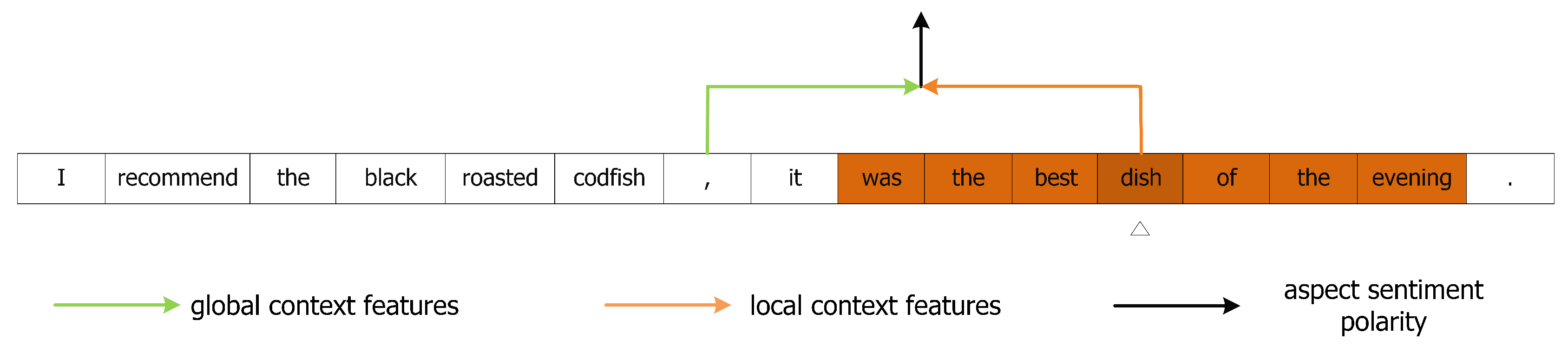
Figure 9.
Dynamic mask for local context features during MHSA encoding process on sample-1. The features of the corresponding positions of local context words in the white boxes will be masked.
Figure 9.
Dynamic mask for local context features during MHSA encoding process on sample-1. The features of the corresponding positions of local context words in the white boxes will be masked.

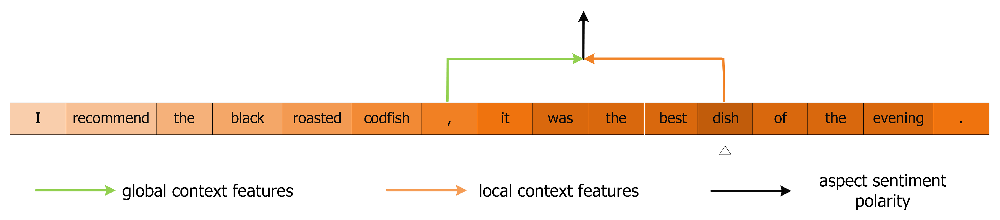
Figure 10.
Dynamic weighted for local context features during MHSA encoding process on sample-1. The chroma of the color indicates the concentration level of the context words.
Figure 10.
Dynamic weighted for local context features during MHSA encoding process on sample-1. The chroma of the color indicates the concentration level of the context words.

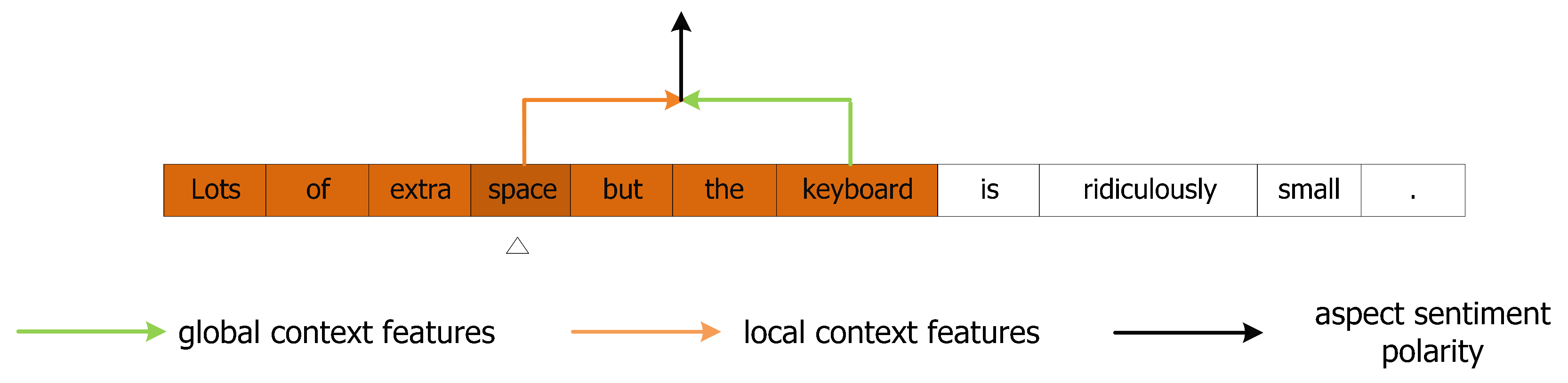
Figure 11.
Dynamic mask for local context features during MHSA encoding process on aspect “space” of sample-2. The features of the corresponding positions of local context words in the white boxes will be masked.
Figure 11.
Dynamic mask for local context features during MHSA encoding process on aspect “space” of sample-2. The features of the corresponding positions of local context words in the white boxes will be masked.

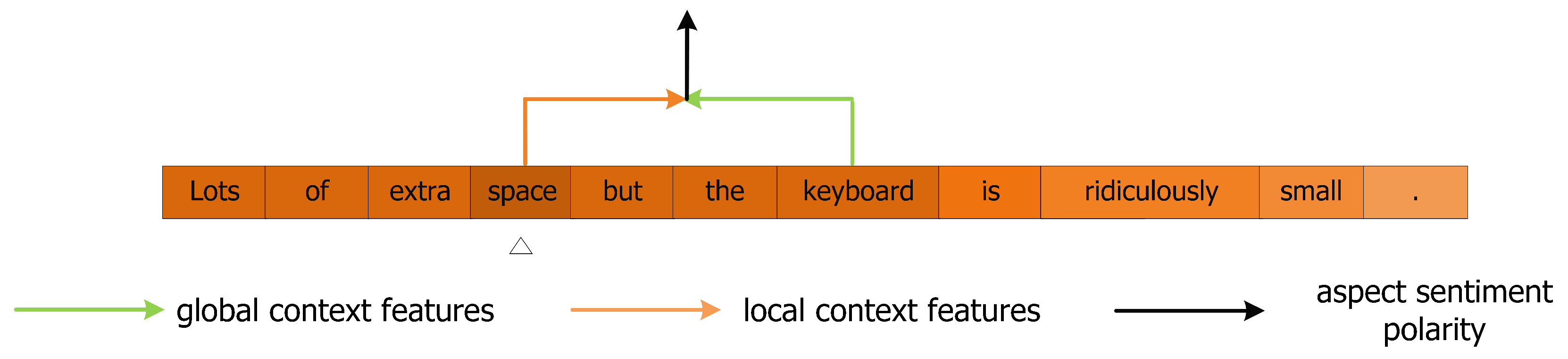
Figure 12.
Dynamic weighted for local context features during MHSA encoding process on aspect “space” of sample-2. The chroma of the color indicates the concentration level of the context words.
Figure 12.
Dynamic weighted for local context features during MHSA encoding process on aspect “space” of sample-2. The chroma of the color indicates the concentration level of the context words.

Figure 13.
Dynamic mask for local context features during MHSA encoding process on aspect “keyboard” of sample-2. The features of the corresponding positions of local context words in the white boxes will be masked.
Figure 13.
Dynamic mask for local context features during MHSA encoding process on aspect “keyboard” of sample-2. The features of the corresponding positions of local context words in the white boxes will be masked.

Figure 14.
Dynamic weighted for local context features during MHSA encoding process on aspect “keyboard” of sample-2. The chroma of the color indicates the concentration level of the context words.
Figure 14.
Dynamic weighted for local context features during MHSA encoding process on aspect “keyboard” of sample-2. The chroma of the color indicates the concentration level of the context words.


Table 1.
Algorithm flow of CDM and CDW mechanism.
| 1 | Accepting the out representation or delivered from local context processor |
| 2 | Calculating the s for each context word regarding to a specific aspect |
| 3 | For CDM mechanism: Constructing the mask matrices M for the input sequence according to s For CDW mechanism: Constructing the weighting matrices W for the input sequence according to s |
| 4 | Applying a matrix element-wise product operation for and M or and M |
| 5 | Output the representation of local context words |
Table 2.
Detail of benchmark datasets.
| Datasets | Positive | Negative | Neural | |||
|---|---|---|---|---|---|---|
| Train | Test | Train | Test | Train | Test | |
| Laptop | 994 | 341 | 870 | 128 | 464 | 169 |
| Restaurant | 2164 | 728 | 807 | 196 | 637 | 196 |
| 1561 | 173 | 1560 | 173 | 3127 | 346 | |
Table 3.
Experimental results of performance. “Glo-CDM” and “Glo-CDW” indicate that both global context and local context participate in the learning process. We set superior SRD thresholds for LCF designs (see Section 4.5.5). We use “ - ” to represent unreported experimental results. The top two scores are in bold.
| Models | Laptop | Restaurant | |||||
|---|---|---|---|---|---|---|---|
| Accuracy (%) | F1 (%) | Accuracy (%) | F1 (%) | Accuracy (%) | F1 (%) | ||
| Baselines | TD-LSTM | 68.13 | - | 75.63 | - | 70.8 | 69 |
| ATAE-LSTM | 68.7 | - | 77.2 | - | - | - | |
| IAN | 72.1 | - | 78.6 | - | - | - | |
| RAM | 74.49 | 71.35 | 80.23 | 70.8 | 69.36 | 67.30 | |
| MGAN | 75.39 | 72.47 | 81.25 | 71.94 | 72.54 | 70.81 | |
| BERT Models | BERT-PT | 78.07 | 75.08 | 84.95 | 76.96 | - | - |
| BERT-SPC | 80.25 | 77.41 | 85.98 | 78.79 | 75.29 | 73.63 | |
| LCF-GloVe | Glo-CDM | 76.02 | 70.58 | 82.5 | 73.92 | 72.25 | 70.92 |
| Glo-CDW | 75.24 | 71.46 | 81.61 | 72.26 | 71.82 | 69.83 | |
| LCF-BERT | Glo-CDM | 82.29 | 79.28 | 86.52 | 80.4 | 76.45 | 75.52 |
| Glo-CDW | 82.45 | 79.59 | 87.14 | 81.74 | 77.31 | 75.78 | |
Table 4.
Results of LCF-GloVe variations of SRD threshold. “Only” means only global context or local context participates in the learning process. “w/o” means “without”. The best scores of LCF-GloVe and LCF-BERT are at the top of the table. SRD thresholds for each variation are equal to basic CDM/CDW design (see Table 5).
| Model | Ablations | Laptop | Restaurant | ||||
|---|---|---|---|---|---|---|---|
| Accuracy (%) | F1 (%) | Accuracy (%) | F1(%) | Accuracy (%) | F1 (%) | ||
| LCF-GloVe | Glo-CDM | 76.02 | 70.58 | 82.5 | 73.92 | 72.25 | 70.92 |
| Glo-CDW | 75.24 | 71.46 | 81.61 | 72.26 | 71.82 | 69.83 | |
| LCF-GolVe | Glo-CDM w/o PFE | 73.04 | 68.17 | 82.32 | 74.32 | 72.83 | 71.09 |
| Glo-CDW w/o PFE | 74.14 | 69.84 | 81.07 | 72.05 | 71.97 | 70.2 | |
| Only Glo | 74.29 | 70.52 | 80.8 | 71.38 | 71.24 | 69.13 | |
| Only CDM | 74.76 | 69.68 | 82.32 | 74.4 | 71.68 | 69.91 | |
| Only CDW | 74.92 | 70.65 | 80.36 | 70.54 | 71.39 | 67.99 | |
| Glo-CDM w/o FIL | 74.14 | 69.25 | 82.23 | 74.02 | 72.25 | 69.57 | |
| Glo-CDW w/o FIL | 74.61 | 69.33 | 80.98 | 71.49 | 71.1 | 69.85 | |
| LCF-BERT | Glo-CDM | 82.29 | 79.28 | 86.52 | 80.4 | 76.45 | 75.52 |
| Glo-CDW | 82.45 | 79.59 | 87.14 | 81.74 | 77.31 | 75.78 | |
| LCF-BERT | Only Glo | 80.88 | 77.52 | 86.25 | 79.56 | 76.16 | 75.01 |
| Only CDM | 80.72 | 76.65 | 83.66 | 75.2 | 75.14 | 74.54 | |
| Only CDW | 81.03 | 77.22 | 84.64 | 77.08 | 75.29 | 73.78 | |
| Glo-CDM w/o FIL | 81.03 | 77.5 | 85.98 | 79.53 | 75.14 | 75.16 | |
| Glo-CDW w/o FIL | 80.56 | 76.23 | 85.98 | 80.08 | 76.3 | 75.16 | |
Table 5.
Recommendations of SRD threshold for LCF-GloVe variations on different datasets.
| LCF TYPE | Laptop | Restaurant | |
|---|---|---|---|
| CDM | 6 | 3 | 3 |
| CDW | 3 | 7 | 5 |
Table 6.
Predictions of three aspects.
| Model | Ablations | Sample-1 | Sample-2 | |
|---|---|---|---|---|
| Dish | Space | Keyboard | ||
| LCF-GloVe | Only Glo | positive | negative | negative |
| Only CDM | positive | positive | negative | |
| Only CDW | neutral | negative | negative | |
| Glo-CDM | positive | positive | negative | |
| Glo-CDW | positive | positive | positive | |
| LCF-BERT | Only Glo | positive | negative | negative |
| Only CDM | positive | positive | negative | |
| Only CDW | positive | positive | negative | |
| Glo-CDM | positive | positive | negative | |
| Glo-CDW | positive | positive | negative | |
© 2019 by the authors. Licensee MDPI, Basel, Switzerland. This article is an open access article distributed under the terms and conditions of the Creative Commons Attribution (CC BY) license (http://creativecommons.org/licenses/by/4.0/).
Share and Cite
MDPI and ACS Style
Zeng, B.; Yang, H.; Xu, R.; Zhou, W.; Han, X. LCF: A Local Context Focus Mechanism for Aspect-Based Sentiment Classification. Appl. Sci. 2019, 9, 3389. https://doi.org/10.3390/app9163389
AMA Style
Zeng B, Yang H, Xu R, Zhou W, Han X. LCF: A Local Context Focus Mechanism for Aspect-Based Sentiment Classification. Applied Sciences. 2019; 9(16):3389. https://doi.org/10.3390/app9163389
Chicago/Turabian StyleZeng, Biqing, Heng Yang, Ruyang Xu, Wu Zhou, and Xuli Han. 2019. "LCF: A Local Context Focus Mechanism for Aspect-Based Sentiment Classification" Applied Sciences 9, no. 16: 3389. https://doi.org/10.3390/app9163389
Note that from the first issue of 2016, this journal uses article numbers instead of page numbers. See further details here.