Support Vector Machine-Based EMG Signal Classification Techniques: A Review
by
 , and
, and
Diana C. Toledo-Pérez
1, 
Juvenal Rodríguez-Reséndiz
2,* ,
,
Roberto A. Gómez-Loenzo
2 and
J. C. Jauregui-Correa
2 1
Facultad de Informática, Universidad Autónoma de Querétaro, 76010 Querétaro, Mexico
2
Facultad de Ingeniería, Universidad Autónoma de Querétaro, 76010 Querétaro, Mexico
*
Author to whom correspondence should be addressed.
Appl. Sci. 2019, 9(20), 4402; https://doi.org/10.3390/app9204402
Submission received: 13 September 2019
/
Revised: 5 October 2019
/
Accepted: 11 October 2019
/
Published: 17 October 2019
(This article belongs to the Special Issue Orthopaedic and Rehabilitation Engineering)
Abstract
:This paper gives an overview of the different research works related to electromyographic signals (EMG) classification based on Support Vector Machines (SVM). The article summarizes the techniques used to make the classification in each reference. Furthermore, it includes the obtained accuracy, the number of signals or channels used, the way the authors made the feature vector, and the type of kernels used. Hence, this article also includes a compilation about the bands used to filter signals, the number of signals recommended, the most commonly used sampling frequencies, and certain features that can create the characteristics of the vector. This research gathers articles related to different kinds of SVM-based classification and other tools for signal processing in the field.
1. Introduction
In recent decades, biomedical signals have been used for communication in Human–Computer Interfaces (HCI) for medical applications; an instance of these signals are the myoelectric signals (MES), which are generated in the muscles of the human body as unidimensional patterns. Because of this, the methods and algorithms developed for pattern recognition in signals can be applied for their analyses once these signals have been sampled and turned into electromyographic (EMG) signals. Additionally, in recent years, many researchers have dedicated their efforts to studying prosthetic control by means of EMG signal classification, that is, by logging a set of MES in a proper range of frequencies to classify the corresponding EMG signals.
The EMG signals are obtained from sensors placed on the skin surface and can help retrieve muscular information during contractions when flexing or extending an articulation. There are also implants placed under the skin that facilitate the signal acquisition, but these are not commonly used.
Regarding the pattern recognition problem for myoelectric control systems, its success depends mostly on the classification accuracy [1] because myoelectric control algorithms are capable of detecting movement intention; therefore, they are mainly used to actuate prostheses for amputees [2].
With the aim of carrying out the pattern recognition for myoelectric applications, a series of features is extracted from the myoelectric signal for classification purposes. The feature classification can be carried out on the time domain or by using other domains such as the frequency domain (also known as the spectral domain), time scale, and time–frequency, amongst others [3].
One of the main methods used for pattern recognition in myoelectric signals is the Support Vector Machines (SVM) technique whose primary function is to identify an n-dimensional hyperplane to separate a set of input feature points into different classes. This technique has the potential to recognize complex patterns [4] and on several occasions it has proven its worth when compared to other classifiers such as Artificial Neural Network (ANN), Linear Discriminant Analysis (LDA) and Particle Swarm Optimization (PSO) [5,6,7,8]. The key concepts underlying the SVM are: (a) the hyperplane separator; (b) the kernel function; (c) the optimal separation hyperplane; and (d) a soft margin (hyperplane tolerance).
A compilation of the most outstanding works that combine different techniques based on SVM is presented in this paper. It also includes a list of those features most commonly used in the time, frequency, time–frequency, and spatial domains for pattern recognition. Finally, other applications of the SVM-based classifier are included in the last section.
2. EMG Signals
Pattern recognition-based myoelectric signal classification consists of logging a specific time interval of EMG signals coming from the muscles and performing many repetitions with different movements, to segment them later. The classification is performed by extracting the features in each interval of the signal to recognize the characteristic information of each movement. From these data, the training is accomplished—which varies according to the method—and, in this way, it is possible to classify the type of movement.
However, the myoelectric signal acquisition is not a simple procedure since the EMG signals have a high noise content since they are not extracted directly from the muscles, but they need to go through the different layers of the skin between the electrode and the pulse generated by the muscle. Besides, the signal acquisition instruments introduce noise themselves by the parasitic frequencies on the power line.
2.1. Signal Acquisition
Due to the acquisition process, it is necessary to make a signal pre-processing step before performing the sample segmentation. This pre-processing stage consists of applying different classes of filters, such as a notch filter to eliminate the power line noise. The noise generated by the skin layers is at frequencies above 500 Hz [1,2,8,9,10,11,12,13,14,15,16,17,18,19,20,21] and at those below 10 Hz [1,9,11,12,14,18,20,22]. Some authors consider that there is noise also in higher frequencies, and thus they use filters that cancel up to 20 Hz [2,6,8,13,15,16,17,19,21,23,24]. Nevertheless, in [7], the authors suppressed frequencies between 90 and 250 Hz and, in [25], the authors removed frequencies lower than 5 Hz and higher than 375 Hz. Table 1 summarizes the band-pass frequency allowed by each study.
Another issue found in the study of myoelectric signals is the frequency at which EMG signals should be sampled—a high frequency could give excess noise, and a lower one could lose a vast amount of information. The sampled frequency most commonly used is 1 kHz [1,9,10,12,13,18,19,27,28,29]. Other authors (e.g., [2,11,22,26,30,31]) use a higher frequency of 1.5, 2, 3, 4, or 10 kHz. In addition, some authors use lower frequencies, such as 500 Hz [15,32]. Table 2 exhibits a recap of the sampling frequencies used by different studies.
Generally, for signal classification, more than one signal is required, because every movement is originated from different parts of the muscle and depends on a number of different muscles; therefore, the use of different channels helps to extract as much information as possible from the action(s) performed by the muscle(s). Among the various studies that have been done, it is common to work with four [1,9,13,23,29,38,39], six [19,40,41], or eight [2,7,11,22,30] channels for the acquisition of the signal; some research papers even work with a smaller number of channels [26,42]. Table 3 depicts an abridgement of the number of channels used by different studies and Table 4 summarizes the electrode type used and the place of electrode placement body. On the other hand, Doulah et al. [33] used a device that includes potentiometers, accelerometers, gyroscopes and force sensors and Lin et al. [43] only used potentiometers to perform their calculations.
The separation between electrode locations is also vital. Most authors recommend a 20 mm distance; however, other authors differ from this opinion since their studies have yielded different results. There are those who indicate that the optimal distance is 10 mm [12] while others point out the optimal distance as 40 mm [55]. At the other extreme, certain authors remark that, when there is more than one channel available to read EMG signals, using a longitudinal channel as well as a transversal one is recommendable.
2.2. Feature extraction from an EMG signal
A parameter of an EMG signal is a stable variable or a value from a mathematical or physical model ideally associated with the generation or detection of an MES process, such as length and depth of a fiber, electrode surface or distance between them, coefficients of the auto-regressive model, etc. [28]. After the signal acquisition stage, a processing stage extracts a series of parameters for the analysis of the EMG signal.
After filtering the signal and digitalizing it, since the vector components do not have any meaning individually but only as a whole, it is necessary to characterize the vector representation of the signal. As a result, it is required to extract the features from the vector that represents the signal, and, from it, implement the vector classification.
A feature of an EMG signal is a unique property, which can be observed or described qualitatively, such as being big or small, fast or slow, and sharp or smooth. An EMG variable is a physical amount that can be computed, reported and transmitted in a numeric form, and that can change as a function of time, such as voltage, frequency, velocity, and delay, amongst others. The variable is estimated during a finite time interval known as an epoch [28].
Nevertheless, when the purpose of extracting the signal features is to control a certain device, it is necessary to obtain more information from each channel of the EMG signal or to assign a control function to a specific combination from the multi-channel system, which is the particular purpose of extracting characteristics from the signals [27].
For the extraction of features, the signals can be processed in the time domain; they can also be transformed into the frequency domain, or represented in the time–frequency space or in time scale. This process consists in assembling a feature vector with different parameters of the signal. Choosing the proper parameters that will form the feature vector correctly is of vital importance since this is the starting point from which classification is made.
That is, an MES is a time function, and, thus, it can be described in terms of its amplitude, frequency, or phase. Hence, for its study, the extracted features lie in different domains, such as time or frequency, and some of their variants. A description of the most common features is given in Appendix A.
2.2.1. Time Domain (TD)
MESs have a very particular structure during muscle contraction, which varies according to the movement performed by the extremity. For this reason, MES classification can be used to actuate a prosthesis. By processing signals in the time domain, there is an increase in the available time for analysis since there is no need for the time-consuming task of transforming the signal to a different domain [27].
Since the signals are usually sampled in the time domain, it is more common to extract features in that domain, since they do not need to be converted and can be processed directly. These time-domain signals are studied in depth and used by researchers from the medical and engineering fields.
Time-domain features are more natural and simpler to extract since they are calculated from the sampled MES time series (the EMG signal) without any intermediate transformation [23,27]. Notwithstanding, time-domain EMG signals also present some disadvantages, which come from the non-stationary properties of the MES, with time-varying statistical properties. Nonetheless, features in this domain are highly used, because of their performance during classification presents a very reduced amount of noise and their processing time is lower compared with those features found in the frequency domain and timescale.
2.2.2. Frequency Domain (FD)
Spectral analysis, also known as representation in the frequency domain, is instrumental in studying muscle fatigue and it is influenced by the firing rate of the motor unit in frequencies lower than 40 Hz and for the morphology of the action potential in muscle fiber in frequencies higher than it [56].
2.2.3. Time–Frequency Domain (TFD)
2.2.4. Spatial Domain (SD)
Spatial Domain features allow finding an improvement in the difference between postures and MES signal force levels, which provide information about the spatial distribution of the motor unit action potential (MUAP) and load between muscles [58].
In theory, a classifier must be able to differentiate, according to the input values, to which class it belongs. An MES is, in essence, a one-dimensional pattern, so that the methods and algorithms developed for pattern recognition can be applied to its analysis. The information extracted from an MES, represented in a feature vector, is chosen to minimize the control error. The feature set should be selected as the one that separates as much as possible the desired output classes [27].
3. Myoelectric Signal Classification
There are many classifiers in the literature, such as Simple Logistic Regression (SLR), Artificial Neural Networks (ANN), Linear Discriminant Analysis (LDA), Naïve Bayes (NB), K-nearest neighbor (KNN), Nonlinear Logistic Regression (NLR), Multi-Layer Perceptron (MLP), and Support Vector Machines (SVM), among others. However, in some cases, such as the ones shown below, the classification of MES with SVM has demonstrated improved performance in terms of accuracy.
Recently, Dhindsa et al. [8] made a performance evaluation of several classifiers, using EMG signals to predict five levels of knee angles. They used 15 features per each of the four measured muscles, combining time and frequency features with four auto-regressive (AR) coefficients. The evaluated classifiers were LDA, NB, KNN, and SVM with different kernels, of which the quadratic kernel of SVM performed the best classification accuracy of %. In addition, in the study, the EMG signals were segmented in five different window sizes with various overlapped window schemes, and the best result was achieved with the overlapping of 500 ms and 250 ms window sizes.
Furthermore, EMG signals can be used for finger movement recognition. Purushothaman and Vikas [6] compared SVM against LDA and NB in the classification of 15 different finger movements from 15 subjects. They utilized Particle Swarm Optimization (PSO) and Ant Colony Optimization (ACO) as feature selection algorithms. MAV, ZC, SSC, and WL were the features extracted (see Appendix A). Remarkably, they achieved more than 95% effectiveness without feature selection using the SVM and 4% less with 16 features considered using PSO and ACO.
EMG signals also allow the diagnosis of muscular dystrophy disorder. Kehri and Awale [25] compared ANN with SVM in the classification of EMG signals to identify this disorder by using a wavelet-based decomposition technique. The results show the classification accuracy of an available clinical EMG database, of 140 samples, with 95% effectiveness using a polynomial kernel of fifth order in an SVM.
A low-cost mechatronics platform for the design and development of robotic hands was proposed by Geethanjali [14], by comparing the SVM with other classifiers, such as ANN, LDA, and SLR. For the database, the subjects performed six different hand movements, and from those signals, the time-domain features were extracted, such as MAV, ZC, SSC, WL, MAVS, VAR, RMS, WAMP, and fourth-order AR coefficients (see Appendix A). With these features, they ensembled five groups to demonstrate their influence. Finally, they applied different kernel functions in the classification with SVM and reached the best result with a linear kernel and normalized data of 92.8% in the group with MAV, SSV, WL, ZC and fourth-order AR coefficients.
3.1. Support Vector Machines
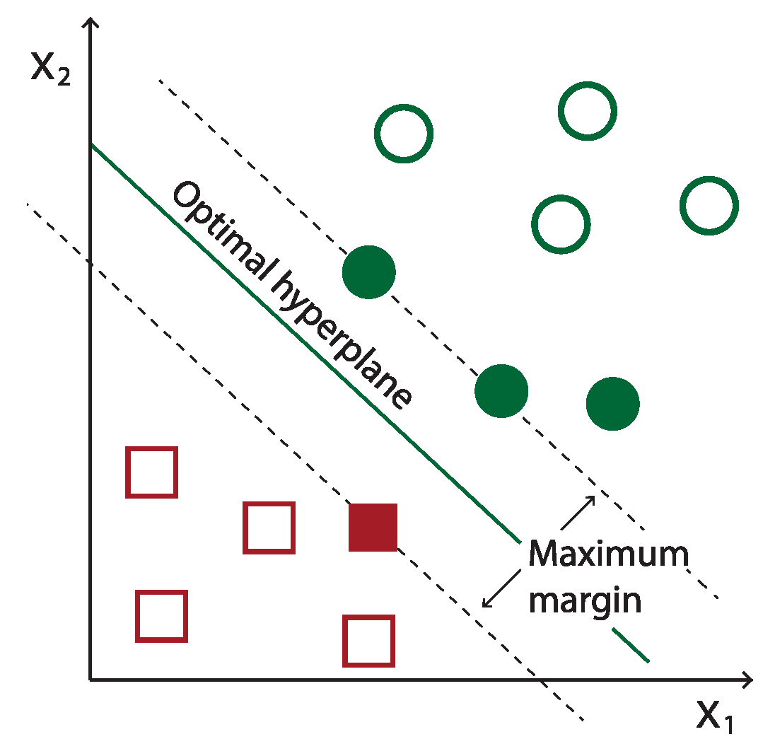
SVM are used quite often as classification algorithms, of body movements, images, sound, etc. SVM construct an optimal separation hyperplane into a feature space that is of high dimension, due to the entries that are mapped using non-linear functions, to distinguish between two (as depicted in Figure 1) or more types of objects. This theory was introduced by Vapnik and Corina in 1995 [59].
For the nonlinear separable problem, the input space is mapped into a high-dimensional feature space and the separation hyperplane is found in this new space. The optimal hyperplane needs to discriminate different categories correctly, and so the hyperplane with maximum clearance between classes them should be found, i.e., the hyperplane that best separates the classes.
In SVM, the training algorithm is reformulated as a problem to solve by Quadratic Programming (QP), whose solution is global and unique. Considering input training data , …, , where corresponds to the input value and to the assigned class ( or ) to which it belongs. If these data are not linearly separable, they are mapped by a non-linear transformation inside of a new feature space where the transformed data will be linearly separable. In this way, the obtained hyperplane that separates object types can be seen as
where and .
The QP problem is supposed to build an optimal hyperplane with a maximum value of separation and a closed error in the training algorithm, that is, we aim to
subject to
If the data points are too close, indeed, if it is difficult to separate them directly, it is possible to use a kernel function K to separate them. That is,
subject to
where is the kernel function, which can be a Radial Basis Function (RBF), a Gaussian, a polynomial, etc. A polynomial kernel can be linear, quadratic, cubic or of any degree d [6], which can be described as
The RBF of two samples, which are feature vectors, is defined by [60]:
The Gaussian function is written as [6]
where and is the standard deviation.
When SVM are used to classify more than two classes, two strategies can be adopted: One Against One (OAO) and One Against All (OAA). The first one discriminates between classes, one by one, that is, the first category compared only against another category and so on, while the second separates each class from the rest.
3.2. SVM-Based Myoelectric Signal Classification
Many researchers have extensively discussed resolution methods for pattern-based classification for control applications. This review only includes works related with SVM, since this method is widely recommended by several authors; this is largely because it is very flexible and can be combined with other methods, which allows improving the accuracy of classification.
For example, in [61], forms of Motor Unit Potentials (MUP) in a Motor Unit Potential Train (MUPT) are evaluated to determinate if they represent a single motor unit They authors obtained 95.6% accuracy with this method.
By taking advantage of technological advances, in [32], the Myo Armband device from Thalmic Lab was placed on 26 subjects to perform a series of four hand gestures, and a linear kernel was used for obtaining an average accuracy of 94.9% with eight electrodes and 72% with four.
Similarly, in [54], a DL-3100 system was used to measure MES signals as a new user authentication method for mobile devices. SVM were trained under four features values (max, min, time of max and min value) and it is possible to choose between five hand gestures to unlock the mobile device. However, in [20], only two channels were used to classify five classes of hand movements, and a method for normalize the signals was implemented, reaching 95% accuracy precision with an expert user.
In [13], two different kernels (Gaussian and RBF) were used to classify five different leg movements, through four MES channels, by combining MAV, WL, ZC and, SSC in such a way that in total 16 different vectors are introduced to SVM. With this method (MKL-SVM), the authors obtained more than 90% of accuracy. In the same manner, in [12,51], an RBF kernel was used for the SVM classifier to perform the error estimation using Leave-One-Out Cross Validation (LOOCV) to separate between six different walking movements; however, the former used 31 electrodes placed on different leg and buttocks muscles to form 16 bipolar signals, while the latter only used 9 electrodes. Both extracted MAV, ZC, WL and, SSC feature signals, but, in [12], the authors also extracted RMS, AR1, AR2 and, AR3. In both studies, 95% precision was obtained.
In time domain, Alkan and Günay [49] combined discriminant analysis with SVM to distinguish between four arm movements. When extracting MAV and AR from windows formed by 32 samples at a sampling frequency of 1 kHz, they made the features vector, with which they obtained an average accuracy of 99%.
Additionally, Liu [22] used AR6, MAV, ZC, WL and SSC to classify six different movements, taking the signals readings in the forearm, by means an incremental learning adaptive algorithm to SVM, which incorporated useful information in tests to a self-correction mechanism to suppress erroneous classifications, with 96.6% average accuracy.
In addition, some studies use MES signals focused on support for people with disabilities. For example, Ishii et al. [45] studied the navigation of an Electric WheelChair (EWC). Four channels of MES signals, placed on cheek, neck, and shoulder, control the seven EWC movements, the iMES of each channel was calculated to form the feature vector. The average classification accuracy was 89.7%.
In the same manner, Rossi et al. [53] took advantage of signals in time domain, therefore they did not use any method for feature extraction. Besides, they combined the information about signal history through the HMM (Hidden Markov Models) with the advantages of time-independent SVM classification, forming an HMM-SVM classification algorithm with 91.8% accuracy to distinguish six different arm movements. Wang et al. [24] implemented visual feedback from the virtual prosthetic hand system to improve classification accuracy and achieved a mean of 98.79%. The authors distinguished between eight movements, with three pairs of sensors, by the SVM classifier and compared the obtained results by using RMS, MAV, VAR, WL, WAM, IAV and SCC as a different features vector.
Sometimes, authors combine features in the time domain with those in the frequency domain. Sasaki et al. [47] developed and tested a tongue interface to detect six motions, including saliva swallowing, from the surface of suprahyoid muscles at the underside of the jaw. They combined RMS from time domain with CC features from frequency domain and achieved % classification accuracy. In addition, Cai et al. [36] performed a classification of eight facial expressions. They used 74 features for each expression using only six channels, and achieved 99.6% of overall accuracy with a cubic kernel in SVM classifier. Among the features used, they included mean value and RMS value of all channels mean values.
Nevertheless, other authors prefer to work in time–frequency domain. Lucas et al. [11] used the representation space of characteristic vector based on DWT (Discrete Wavelet Transform), by using an unrestricted parametrization of Wavelet mother. With this method, they obtained an average classification error of six hand movements, through eight electrodes, of %. Using the same method, Lin et al. [43] utilized a pair of features after applying DWT in their MES raw data, from eight subjects, to identify the movement intention of the patients. They found as the best choice the fifth step in DWT decomposition combined with MAV and Max features, which achieved 100% accuracy with SVM classifier.
In addition, Too et al. [21] classified 17 hand and wrist movements from MES signals acquired from NinaPro database. The feature vector was composed of RMS extracted from DWT and the average energy of spectrogram at each frequency bin, after having applied a Principal Component Analysis (PCA) and conserving the first three. By applying SVM, the highest classification accuracy was 95% and 71.3% for normally-limbed and amputee subjects, respectively. Moreover, Ahlawat et al. [17] used PCA for dimensionality reduction with a kernel quadratic in SVM classifier, where kurtosis, skewness, SSC, MAV and AR1 in TD were the features extracted. The overall mean classification accuracy was 99.04% for the two activities performed.
At the other extreme, Omari and Liu [39] proposed an algorithm called GAPSO-SVM that combines Genetic Algorithm (GA) and Particle Swarm Optimization (PSO) combined with SVM. The algorithm selected optimal parameters for RBF and an optimal decomposition level also making use wavelet mother function to classify energy of wavelet coefficient obtained from forearm signals. In addition, they implemented PCA, and obtained 98.7% accuracy in the classification. As in the previous study, Sui et al. [46] used PSO but they combined it with an improved SVM (by removing slack variables, as the bias value from the decision function), calling their method PSO-ISVM, which effectively identified six types of upper limb movements with an average recognition rate of 90.66%. As a feature vector, the WPT was used to extract the variance and energy of the wavelet packet coefficients and, as a kernel, the RBF.
In the same manner, Xing et al. [50] used the energy node of WPT coefficients as MES signal characteristic. They also used the Non-parametric Weighted Feature Extraction (NWFE) to reduce the dimensionality of features vector that enters the SVM, from which they obtained 98.39% precision in OAA mode, and 98.214% in OAO mode. After the analysis and comparison between different mother wavelet functions in discrete and continuous time, Too et al. [37] achieved 98.74% using MAV feature in Symlet 4 function in level 2, 98.49% by applying WL feature in Coif 3 function in level 4, both from DWT. For CWT, 98.56% was achieved with MAV by employing Sym 6, scale 16 and 98.64% with WL by using Mexh, scale 32. The authors classified 10 different hand movements with four channels.
Another method that is used to reduce the dimensionality problem is that used by Erkilinc and Sahin [48], which, in addition to applying FFT to four MES signals for the camera control, whose movements are up, downright, left and neutral, performs a component reduction by SPCA (Sparse Principal Component Analysis), before entering SVM values. The authors implemented a not widely used technique, namely the data division in Kaiser windows, obtaining 81% accuracy. In the same manner, Goen and Tiwari [5] employed SPCA with the lasso to produce modified principal components with scattered loads. In addition, they used the SVM ensemble for classification of seven different arm movements, combined with a window length of 256 ms and a 50% overlapping. The classification accuracy obtained by the authors reached 98%.
Unlike other authors, Kouchaki et al. [62] simulated, in the laboratory of the University of Waterloo, MES signals by incorporating statistical and morphological properties. They utilized SVM to discriminate between different neuromuscular diseases (neuropathy and myopathy), and, after simulating signals, decomposed them by using an Empirical Mode Decomposition (EMD) as well as the Kolmogorov complexity and other informative features to reveal the number of irregularities within each subspace formed by EMD. The accuracy obtained was 91.11%.
Combining time and frequency domain features, Yoshikawa et al. [35] used ZC in time domain and mean MES, CC and, DCC (Delta Cepstrum Coefficients) in frequency domain. The last one is defined as a characteristic of the dynamic type, and it is the difference between two CC. The features were used to classify seven hand movements, and they obtained a precision of 91–94.4%, depending on the test subject. This classification was used for digital robotic arm control, with 62.5 Hz delay. In addition, Doulah et al. [33] presented a method for automatic detection of posture transition and used it for a knee-ankle-foot orthosis. Furthermore, they used a PCA for dimensionality reduction from the eleven extracted features of ten subjects with 14 sensors (MAV, SSC, STD, entropy, coefficient of variation, maximum, minimum, median, maximum to RMS ratio, RMS to mean ratio, and fractal dimension). The obtained precision was 92.94% for the detection of the sit-to-stand posture transition.
In the same way, Bian et al. [15] compounded IEMG, STD and RMS features in time domain and MPF and MNF in frequency domain. Besides using a linear kernel, the dimensionality reduction was done by PCA. Starting from seven vectors, the obtained results were higher than 92.25% for classifying eight movements, whose signals were extracted using the eight channels from Myo armband device. Furthermore, Roldan-Vasco et al. [7] combined five time domain features (LOG, DASDV, VAR, ZC and MYOP) with two in frequency domain (MNF and FR) to record the activity from 47 healthy subjects when swallowing water, yogurt and saliva, using for classification SVM with RBF kernel, and obtained 92.03% accuracy.
Moreover, without feature extraction tools, Luo et al. [19] extracted the synergistic patterns of myoelectrical activities by a non-negative matrix factorization (NMF), with five healthy subjects, to classify five different movements (hand open and close, key pinch, palm valgus and grasp cylindrical tool). They implemented two different filters, one analog and one digital, within the recorded signals from six muscles. By their method, the muscle synergy patterns as a feature vector matrix could achieve the mean classification rate of 96.08%.
Table 5 lists classification accuracy according to each one of the authors mentioned above, who worked with time-domain features. Number of classes and channels are in the second and third column, respectively. The features extracted from EMG signals are in the third column and, in the last column, the classification accuracy obtained is presented. Table 6 summarizes those who worked in time–frequency domain, while Table 7 presents the authors who combined features in different domains.
3.3. Other Applications of SVM-Based Classifiers
To identify abnormal changes in Mental Workload (MWL) and thus prevent accidents due to work overload, Yin and Zhang [63] classified overload levels (low, medium and high) using EEG-PSD to form the features vector. To reduce it, they used the Locally Linear Embedding (LLE) technique, and subsequently classified with combined techniques of Support Vector Clustering (SVC) and Support Vector Data Description (SVDD), obtaining 79.54% accuracy. In the same year, Yin and Zhang [64] used LS-SVM to differentiate between the state of high mental load and fatigue, by combining EEG, ECG, and Electrooculogram (EOG) signals, with a feature reduction made with a Recursive Feature Elimination (FRE) and keeping RBF kernel. This procedure improved the accuracy to 92.67% compared against their previous study.
The classification of other types of signals has also been utilized as a guide for some doctors and therapists for the detection of different diseases, or the diagnosis of disorders in the motor system. In [65], an adaptive system for SVM, called ASVM, is proposed to diagnose diseases through the blood, using data on diabetes and breast cancer. In this method, the bias value of SVM is adjusted by a feedback mechanism, which allows the classification to be done more quickly and with higher precision than in its different evaluation, obtaining 67.22–97.39% accuracy.
Similarly, features in temporal and frequency space were utilized in [66] to perform the detection of muscular fatigue of the lower extremities to prevent falls and injuries; with the aid of six cameras, the authors differentiated between the state of fatigue and without fatigue using SVM with linear and RBF kernel, obtaining 96% accuracy with both kernels. In the same manner, in [67], six cameras with a 200 Hz sample rate were used to differentiate between assisted walking of patients with arm support and unassisted walking. The authors also used temporal space features, combining Non-dominated Sorting Genetic Algorithm II (NSGAII) and Genetic Algorithms (GA) with SVM to choose from among 30 marching parameters and conducted the classification, obtaining 99.31% precision.
Other authors (e.g., ) combined different signal types, such as EEG, ECG, EOG, EGM and videotaping for sleep evaluation, i.e., distinguishing between the state of waking and sleep of different people. The features used by Park et al. [68] were Proportional Integration Mode (PIM), Zero Crossings Mode (ZCM) and FFT, to which RBF is applied and then classified with the SVM, obtaining a precision of 88.94%.
More techniques utilized by some authors also reduced the number of features to improve the classification accuracy and to increase the processing speed by reducing the dimensionality of the features vector; for instance, in [69], an approach of random forest classification to the diagnosis of lymphatic diseases is proposed. In the first stage, the authors performed a features reduction of different methods, obtaining as best result 92.2% accuracy in the distinction of four states of the patient, including normal, malignant lymph or fibrosis, with the reduction from 18 to 6 features using genetic algorithms.
Khazaee and Ebrahimzadeh [70] used ECG signals to differentiate between five kinds of arrhythmias. They used a database offered by MIT-BIH. The procedure was performed in three different stages. The first one consisted in feature extraction by Non-Parametric Power Spectral Density (NPPSD). In the second, the classification using SVM with Gaussian Radial Basis Function was performed. Finally, they accomplished the SVM parameter optimization by a GA. The classification accuracy obtained was 96%.
Raj and Ray [42] differentiated arrhythmias using PCA to reduce features in time–frequency space. These features were obtained from ECG by means of the Discrete Orthonormal Stockwell Transform (DOST) concatenated with morphological features. They also employed the PSO technique to adjust the SVM parameters with an RBF kernel. These combined methods, PSO and SVM, reached 98.82% classification accuracy to differentiate among 16 types of arrhythmic events that are produced more frequently in the heart.
Dobrowolski et al. [71] used the SVM for neuromuscular disorder diagnosis based on the analysis of scalograms formed from MES extracted from the deltoid muscle. Then, the SVM analysis was implemented to subsequently reduce to a single decision parameter. The error probability of this method was 0.5%.
Another medical application where an SVM is used for classification is in the differentiation of four main classes in which a protein is composed. In [72], a method is proposed to discriminate between both classes and protein structures by the incorporation of pseudo average chemical shift along with an SVM. This method was used onin four different databases, obtaining 84.2%, 85%, 86.4%, and 89.2%, respectively, in classification accuracy.
In the case of hyperspectral image classification, in [73], a guided filter is incorporated into the SVM classifier. This originates from the fusion of spectral and spatial features with the help of the PCA method. The authors classified more than nine classes with the spatial features of the SVM and achieved an average 98.92% classification accuracy.
Other images that also have been classified are digital mammograms, in search of microcalcifications for diseases prevention. For instance, El-Naqa et al. [74] used a database of 76 digital mammograms, and the obtained accuracy with a polynomial kernel in SVM was 94%.
The authors of [39,60] used GA combined with SVM to classify images obtained by fusing multifrequency RADARSAT-2 synthetic aperture radar and Thaichote multispectral images. The results provided high classification accuracy at over 95%.
The Content-Based Image Retrieval (CBIR) technique, which is a developing trend in digital image processing, aims at recovering a queried image from a large database. In this field, Sugamya et al. [75], in the search for an image, extracted color, form and texture from an image, and later they used SVM for the classification, obtaining 76.6% accuracy with the help of the standardized Euclidean metric.
Moreover, in addition to extracting voltage signals from the brain, images can also be extracted. Alam et al. [76] differentiated between healthy individuals and those who suffer from Alzheimer’s disease. They used structural Magnetic Resonance Imaging (sMRI) data, from which a features extraction was done with the aid of Voxel-Based Morphometry (VBM), and the features reduction with the PCA. Finally, the classification accuracy was 84.17%.
Sharma and Srivastava [77] used SVM to classify characters strings, i.e., text classification. The fact that such character strings did not have the proper format to be classified was solved with the help of the Stemmers–Stemming algorithm. For classification, they uses RBF kernel, with LibSVM to distinguish between related phrases with shopping and food, obtaining a correct classification of 64.86%.
Other signals frequently used are those of digital modulation. For example, Zhou [78] used second-, fourth- and sixth-order cumulants as signal features, and also employed an RBF kernel combined with a method of cross-validation grid parameters selection to improve the SVM-based classification accuracy, reaching 92.2%.
4. Conclusions
Pattern classification is used in certain areas of knowledge. Depending on the needs and characteristics of each system, a specific tool may be selected. SVM offer a high classification accuracy since they allow the combination with other pattern classification methods to reach different objectives that are taken in the classification, besides a high accuracy percentage. In other words, it allows the incorporation of tools that transform the input data to the SVM or that solve the same.
The mentioned authors combined methods to improve the classification accuracy in different applications, although the main purpose of the article is making a compilation of those studies which used myoelectric signals as input vector. In addition, other applications of classification based on SVM are listed to give the reader a broader idea of different fields of study in which the SVM can be applied. Then, four points can be concluded:
- The most common kernel used was RBF, followed by linear and Gaussian.
- PCA is the most common tool for dimensionality reduction.
- MAV, SSC, ZC and WL are the most utilized time-domain features.
- Many channels are not necessary to obtain good precision.
Most of the published papers seek advantage in feature extraction area, but only certain researchers reported an algorithm to combine directly with the SVM. An example of this is the combination with GA [39,67,70,79]. Therefore, this is an area of opportunity, as there are several algorithms in artificial intelligence that can be tested and combined with SVM.
Another small studied tool is, instead of using feature reduction algorithms such as PCA or SPCA, decreasing the number of input vectors when one has many features extracted; in such case, feature extraction algorithms can be used. Currently, these algorithms are mainly used in data mining.
Author Contributions
Conceptualization, D.C.T.-P. and J.R.-R.; Methodology, D.C.T.-P.; Software, D.C.T.-P.; Validation, D.C.T.-P. and J.C.J.-C.; Formal analysis, D.C.T.-P.; Investigation and Visualization, D.C.T.-P. and J.R.-R.; Data curation, D.C.T.-P., and J.C.J.-C.; Writing—original draft preparation, Writing—original draft, review & editing, all the authors.
Funding
CONACYT paid for scholarship 561144 for this research.
Acknowledgments
We would like to thank the Graduate Studies Division from the Faculty of Informatics at Universidad Autónoma de Querétaro by enabling C.L. to carry out this Ph.D. research.
Conflicts of Interest
The authors declare no conflict of interest.
Abbreviations
The following abbreviations are used in this manuscript:
| AAC | Average Amplitude Change |
| AAV | Average Absolute Value |
| ACO | Ant Colony Optimization |
| AFB | Amplitude of the First Burst |
| ANN | Artificial Neural Network |
| AR | Auto-Regressive |
| CC | Cepstrum Coefficients |
| CBIR | Content-Based Image Retrieval |
| COF | Coefficient of variation |
| Com1 | Mean value of all channels’ mean values considered. |
| Com2 | RMS value of all channels’ mean values considered. |
| CWT | Continuous Wavelet Transform |
| DASDV | Difference of Absolute Standard Deviation |
| DCC | Delta Cepstrum Coefficients |
| DFT | Discrete Fourier Transform |
| DWT | Discrete Wavelet Transform |
| ECG | Electrocardiogram |
| EEG | Electroencephalogram |
| EGM | Electrogram |
| EMD | Empirical Mode Decomposition |
| EMG | Electromyography |
| ENT | Entropy |
| EOG | Electrooculogram |
| EWC | Electric WheelChair |
| FD | Frequency Domain |
| FFT | Fast Fourier Transform |
| FMD | Frequency Median Density |
| FMN | Frequency Mean Density |
| FRD | Fractal Dimension |
| GA | Genetic Algorithm |
| HCI | Human-Computer Interface |
| HIST | Histogram |
| HMM | Hidden Markov Models |
| FR | Frequency Ratio |
| IAV | Integrated Absolute Value |
| IEMG | Integrated Electromyography Signal |
| ISVM | Improved Support Vector Machine |
| KNN | K-Nearest Neighbour |
| LDA | Linear Discriminant Analysis |
| LLE | Locally Linear Embedding |
| LOG | Log-Detector |
| LOOCV | Leave-One-Out Cross Validation |
| MAV | Mean Absolute Value |
| MAVS | Mean Absolute Value Slope |
| MAVSLP | Differences between Mean Absolute Value |
| MAX | Maximum Value |
| MDV | Median Differenital Value |
| MDF | Median Frequency |
| MED | Median |
| MES | Myoelectric Signals |
| MHW | Multiple Hamming Windows |
| MIN | Minimum Value |
| MKL | Multiple Kernel Learning |
| MLP | Multi-Layer Perceptron |
| MMAV1 | Modified Mean Absolute Valye type 1 |
| MMAV1 | Modified Mean Absolute Valye type 2 |
| MNF | Mean Frequency |
| MNP | Mean Power |
| MTW | Multiple Trapezoidal Windows |
| MUP | Motor Unit Potentials |
| MUPT | Motor Unit Potential Train |
| MWL | Mental WorkLoad |
| MYOP | Myopulse Percentage rate |
| NB | Naive Bayes |
| NLR | Non-linear Logistic Regression |
| NMF | Non-negative Matrix Factorization |
| NOR | Norm |
| NPPSD | Non-Parametric Power Spectral Density |
| NSGAII | Nondominated Sorting Genetic Algorithm II |
| NWFE | Non-parametric Weighted Feature Extraction |
| OAA | One Against All |
| OAO | One Against One |
| PCA | Principal Component Analysis |
| PIM | Proportional Integration Mode |
| PKF | Peak Frequency |
| PSO | Particle Swarm Optimization |
| PSD | Power Spectral Density |
| PSR | Power Spectrum Ratio |
| QP | Quadratic Programming |
| RAN | Range |
| RBF | Radial Basis Function |
| RFE | Recursive Feature Elimination |
| RMS | Root Mean Square Value |
| SD | Spatial Domain |
| SLR | Simple Logistic Regression |
| sMRI | structural Magnetic Resonance Imaging |
| STD | Standard Deviation |
| STFT | Short Time Fourier Density |
| SPCA | Sparse Principal Component Analysis |
| SSC | Slope Sign Changes |
| SSI | Simple Square Integral |
| SVC | Support Vector Clustering |
| SVDD | Support Vector Data Description |
| SVM | Support Vector Machines |
| SUM | Summation |
| SWT | Stationary Wavelet Transform |
| TD | Time Domain |
| TFD | Time–Frequency Domain |
| TTP | Total Power |
| TVAR | Time Varying Auto Regressive |
| VAR | Variance |
| VBM | Voxel-Based Morphometry |
| v-Order | V |
| WAMP | Willson Amplitude |
| WL | Waveform Length |
| WPT | Wavelet Packet Transform |
| ZC | Zero Crossings |
| ZCM | Zero Crossings Mode |
Appendix A. Common Features
Appendix A.1. Time Domain
- Average Amplitude Value (AAV)
- Mean Absolute Value (MAV)MAV is one of the most used statistics in signal analysis [27], and it can be described as
- Modified Mean Absolute Value type 1 (MMAV1)This is a MAV generalization [82] where a weighted window function is used in the MAV equation with the purpose to make it more robust; it is computed aswhere
- Modified Mean Absolute Value type 2 (MMAV2)This is another MAV generalization, such as MMAV1 [82], where the weight function is continuous, which improves the smoothness of the weighted function. It is given bywhere
- Simple Square Integral (SSI)This feature corresponds to the signal energy [38], that is, SSI is the sum of squared values of the EMG signal amplitude, it can be expressed as:
- Variance (VAR)This statistic is another power index [52], and is defined as the mean of the squared values of the deviation from the mean of the variable; it can be expressed as
- Zero Crossings (ZC)A simple measure of frequency can be obtained by counting the number of times that the wave crosses by zero [27]. To reduce the noise effects, a lower bound for the absolute difference could be included as a threshold L. Given two consecutive samples and , ZC is the count of the zero crossings, that is,whereThis algorithm will fail to log a zero crossing if the absolute difference of two consecutive samples of opposite sign are lower than the selected threshold.
- Slope Sign Changes (SSC)This feature allows another description of the frequency; it is the number of times that a slope sign change occurs [27]. Again, an adequate threshold can be chosen to reduce the induced noise. Given three consecutive samples , and , the SSC count is increased ifwhere
- Waveform Length (WL)WL provides information about the complexity of the waveform in each segment [27]; this is simply the accumulated waveform length above time segment defined as
- Average Amplitude Change (AAC)AAC is the mean value of the absolute difference between two consecutive samples [80], that is,
- Willson Amplitude (WAMP)WAMP is an EMG signal frequency information measure. It is the number of times the amplitude of the absolute difference between two contiguous samples exceeds a preset lower bound L. This is related with the triggering of the action potentials of motor unit and muscle contraction force. It is defined aswhere
- Root Mean Square Value (RSM)RMS is modeled as a Gaussian random process with modulated amplitude, which is related to a constant force and contraction without fatigue; it is very similar to the calculation of the standard deviation since it is given by
- Integrated EMG (IEMG)Some features such as the IEMG also allow signal recognition without a pattern. This is used as an initial detection rate and it is related to the trigger point of the EMG signal sequence. It is defined as the sum of the absolute values of each EMG sample, and it can be expressed as [83]:
- Auto-Regressive Coefficients (AR)The AR form a prediction model that describes each EMG signal sample as a linear combination of the previous samples , …, plus a white noise error term ; this model is expressed aswhere P is the order of the AR model. The most common P used is 6 [10,22,23,28]; nevertheless, some authors [12] used orders 1, 2 and 3, while Villarejo Mayor et al. [26] used .
- Standard Deviation (STD)STD is defined as the square root of the variance, that is,where is the AAV.
- Difference of Absolute Standard Deviation (DASDV)DASDV is similar to RMS since it is the standard deviation from wavelength [84]; it is defined by
- Log-Detector (LOG)
- Myopulse Percentage rate (MYOP)MYOP is a myopulse output averaged value, which is defined as “1” when the EMG signal absolute value exceeds a determined lower bound L [81]. Mathematically, it is calculated by:where
- Absolute Value of the Third, Fourth and Fifth Temporal Moments (TM3, TM4 and TM5)Temporal moment is a statistical analysis proposed by Saridis and Gootee [86]. The first and the second temporal moments are the absolute values of AAV and VAR, and the next three are defined as
- Histogram (HIST)This feature parts elements in EMG signal into M segments, which have to be equally spaced. Finally, HIST returns a number of signal elements for each segment [82]. A suggested number for M is 9.
- v-Order (V)V is a non-linear detector that computes implicitly the strength of a muscular contraction. It is defined from a functional mathematical model of EMG signal generation, given by the expressionwhere and are constants and is a class of the ergodic Gaussian processes; is theoretically 0.5, but a rate between 1 and 1.75 was obtained experimentally [87]. An optimal value for V has been reported as 2 [85], which leads to the same definition of RMS. The mathematical definition of V is
- Mean Absolute Value Slope (MAVSLP)MAVSLP is a by-product of MAV; it computes differences between adjacent MAV segments [88]. Its equation is given bywhere , …, I is the number of segments covering the EMG signal. However, with a higher number of segments, its definition approaches that of a traditional MAV feature. In the study of Miller [88], I is set to 3.
- Multiple Hamming Windows (MHW)MHW segments the raw EMG signal by a series of Hamming windows [89]. The MHW features are computed using the energy of each window, which can be expressed asfor , …, I, where w is the Hamming windowing function. Similar to MAVSLP, it is recommended to have a small I; for example, in [90], it is set to 3 and the authors suggested using a 30% overlap.
- Multiple Trapezoidal Windows (MTW)MTW is similar to MHW since it also uses the contained energy inside a window but, instead of using Hamming windows, it uses trapezoidal windows and is described byfor , …, I. As in the case of MHW, I is set to 3 with the same overlapped windows [90].
- Median Differential Value (MDV)It is the mean value of the differential value of all peak values of the EMG signal. MDV is described by [36]:
- Amplitude of the First Burst (AFB)AFB is defined as the first maximum point extracted from the resulting time function [90]. To calculate it, the raw EMG signal is first squared and passed through a moving mean FIR filter with a Hamming windowing function, and then the low-frequency components of the EMG signal are obtained. The maximum value of the first burst is used as a feature [82].
Appendix A.1.1. Frequency Domain
- Mean Frequency (MNF)It is a mean frequency which is calculated as the sum of the product of the MES signal power spectrum and the frequency divided by the total of the spectrum intensity [23]. In addition, it is known as central frequency or spectral center of gravity [38].where is the spectral frequency in the bin of frequency l, is the EMG signal power spectrum in the bin l, and M is the frequency bin length.
- Median Frequency (MDF)It is the frequency divided into two regions with the same amplitude; that is to say, MDF is the total power average [23], and could be expressed as the number MDF with the property thatwhere is the EMG signal power spectrum at a frequency bin l, and M is the frequency bin length.
- Peak Frequency (PKF)It is the frequency at which maximum power occurs, described by
- Mean Power (MNP)MNP is the mean power of the EMG power spectrum. It is calculated as
- Total Power (TTP)It is defined as an aggregate of the EMG signal frequency spectrum or as zero spectrum moment, and is given by
- Frequency Ratio (FR)FR can be used to make a distinction between muscle contraction and relaxation [91], which uses the quotient obtained from the division of low-frequency EMG components with high frequency. The equation that defines it is expressed by:where ULC and LLC are upper and lower coefficients of the cutoff frequency of the low band frequency and UHC and LHC are those from the high frequency, respectively.The threshold to divide between low and high frequencies can be determined of two different ways, the first suggested by Han et al. [92], who used a range of 30–250 Hz for low frequency and 250–1000 Hz of high frequency. The values were obtained by experiments. The second was suggested by Oskoei and Hu [91], who proposed obtaining the frequency rates based on the MNF value.
- Power Spectrum Ratio (PSR)The PSR can be defined as an extended version of the PKF and the FR [93]. It is the quotient between that is close to the maximum value of MES power spectrum and P that is the total energy of MES power spectrum. It can be defined mathematically bywherewith the PKF value and n the MES integral limit. Qingju and Zhizeng [93] defined and P in 10 and 500 Hz.
- The First, Second and Third Spectral MovementsAnother statistic that is offered to MES spectral power analysis is the moment spectral. The first three moments are the most important [38]. These are calculated by
- Variance of Central Frequency (VCF)It is defined by the use of some moment spectral and is written aswhere is the central frequency.
- Power Spectral Density (PSD)It is defined as the energy distribution or power signal over the different frequencies of which it is formed. Mathematically, it is defined aswhere is the Fourier Transform; the integral of this function in the whole axis f is the total energy value of , the signal.
- Frequency Median Density (FMD)FMD splits PSD into two equal parts and is defined as
- Frequency Mean Density (FMN)FMN is the frequency mean of the PSD and is described by
- Cepstrum Coefficients (CC)CC is the inverse of Fourier transform of the logarithmic power spectrum of a signal. Low-order coefficients are often used in speech recognition classification [35]. If for is defined as Fourier transform, when the sample measured nth from the signal , from the source lth, the Fourier transform isThen, W, being a CC characteristic parameter, is defined aswhere
Appendix A.1.2. Time–Frequency Domain (TFD)
- Short Time Fourier Transform (STFT)STFT corresponds to the fast Fourier transform, which mathematically can be expressed as follows:with g as window function, k as time sample and m as frequency bins.
- Continuous Wavelet Transform (CWT)CWT is the wavelet transform of a continuous signal.with t as translation parameter, a as scale parameter and as mother wavelet function.
- Discrete Wavelet Transform (DWT)DWT divides the signal into an approximation and detail coefficient by passing through low and high as complementary filters. The approximation coefficients are divided into second-level approximation detail coefficients. By repeating the process, a signal is divided into many components of lower resolution.
- Wavelet Packet Transform (WPT)WPT is a DWT generalized version that applies to both low-pass results (approximations) and high-pass results (details).
- Stationary Wavelet Transform (SWT)SWT does not decimate the signal in each stage, avoiding non-linear distortion problem of DWT and WPT. Hakonen et al. [58] pointed out that Wavelet transforms allow focusing on specific frequency bands because of their use of subsets of coefficients, which could provide better robustness to the system, as in comparison with TD and DF features. Additionally, the TFD features generate a high dimension feature vector; therefore, dimensionality reduction is usually necessary so that, when using this vector, the speed can be increased.
Appendix A.1.3. Spatial Domain (SD)
- Experimental VariogramThe variogram function describes the spatial correlation between observations. The variogram definition is based on the idea that the z value depends on the location where x is observed.where h is the distance vector, is the measurement at location and is the number of pairs h units apart from the direction of the vector h.
References
- Englehart, K.; Hudgin, B.; Parker, P. A wavelet-based continuous classification scheme for multifunction myoelectric control. IEEE Trans. Biomed. Eng. 2001, 48, 302–311. [Google Scholar] [CrossRef] [PubMed]
- Miller, J.D.; Beazer, M.S.; Hahn, M.E. Myoelectric Walking Mode Classification for Transtibial Amputees. IEEE Trans. Biomed. Eng. 2013, 60, 2745–2750. [Google Scholar] [CrossRef] [PubMed]
- Oskoei, M.; Hu, H. Myoelectric Control Systems - A Survey. Biomed. Signal Process. Control. 2007, 2, 275–294. [Google Scholar] [CrossRef]
- Oskoei, M.; Hu, H. Support vector machine-based classification scheme for myoelectric control applied to upper limb. IEEE Trans. Biomed. Eng. 2008, 55, 1956–1965. [Google Scholar] [CrossRef]
- Goen, A.; Tiwari, D.C. Classification of the Myoelectric Signals of Movement of Forearms for Prosthetic Control. J. Med. Bioeng. 2016, 5, 76–84. [Google Scholar] [CrossRef]
- Purushothaman, G.; Vikas, R. Identification of a feature selection based pattern recognition scheme for finger movement recognition from multichannel EMG signals. Australas. Phys. Eng. Sci. Med. 2018, 41, 549–559. [Google Scholar] [CrossRef]
- Roldan-Vasco, S.; Restrepo-Agudelo, S.; Valencia-Martinez, Y.; Orozco-Duque, A. Automatic detection of oral and pharyngeal phases in swallowing using classification algorithms and multichannel EMG. J. Electromyogr. Kinesiol. 2018, 43. [Google Scholar] [CrossRef]
- Dhindsa, I.S.; Agarwal, R.; Ryait, H.S. Performance evaluation of various classifiers for predicting knee angle from electromyography signals. Expert Syst. 2019, 36, 1–14. [Google Scholar] [CrossRef]
- Englehart, K.; Hudgins, B. A robust, real-time control scheme for multifunction myoelectric control. IEEE Trans. Biomed. Eng. 2003, 50, 848–854. [Google Scholar] [CrossRef]
- Huang, Y.; Englehart, K.B.; Hudgins, B.; Chan, A.D.C. A Gaussian mixture model based classification scheme for myoelectric control of powered upper limb prostheses. IEEE Trans. Biomed. Eng. 2005, 52, 1801–1811. [Google Scholar] [CrossRef]
- Lucas, M.F.; Gaufriau, A.; Pascual, S.; Doncarli, C.; Farina, D. Multi-channel surface EMG classification using support vector machines and signal-based wavelet optimization. Biomed. Signal Process. Control 2008, 3, 169–174. [Google Scholar] [CrossRef]
- Ceseracciu, E.; Reggiani, M.; Sawacha, Z.; Sartori, M.; Spolaor, F.; Cobelli, C.; Pagello, E. SVM classification of locomotion modes using surface electromyography for applications in rehabilitation robotics. In Proceedings of the 19th International Symposium in Robot and Human Interactive Communication, Viareggio, Italy, 13–15 September 2010; pp. 165–170. [Google Scholar] [CrossRef]
- She, Q.; Luo, Z.; Meng, M.; Xu, P. Multiple kernel learning SVM-based EMG pattern classification for lower limb control. In Proceedings of the 2010 11th International Conference on Control Automation Robotics Vision (ICARCV), Singapore, 7–10 December 2010; pp. 2109–2113. [Google Scholar] [CrossRef]
- Geethanjali, P. A mechatronics platform to study prosthetic hand control using EMG signals. Australas. Phys. Eng. Sci. Med. 2016, 39, 765–771. [Google Scholar] [CrossRef] [PubMed]
- Bian, F.; Li, R.; Liang, P. SVM based simultaneous hand movements classification using sEMG signals. In Proceedings of the 2017 IEEE International Conference on Mechatronics and Automation (ICMA), Takamatsu, Japan, 6–9 August 2017; pp. 427–432. [Google Scholar] [CrossRef]
- Powar, O.S.; Chemmangat, K. Feature selection for myoelectric pattern recognition using two channel surface electromyography signals. In Proceedings of the TENCON 2017—2017 IEEE Region 10 Conference, Penang, Malaysia, 5–8 November 2017; pp. 1022–1026. [Google Scholar] [CrossRef]
- Ahawat, V.; Narayan, Y.; Thakur, R. Support vector machine based classification improvement for EMG signals using principal component analysis. J. Eng. Appl. Sci. 2018, 13, 6341–6345. [Google Scholar] [CrossRef]
- Ibrahim Aly, H.; Youssef, S.; Fathy, C. Hybrid Brain Computer Interface for Movement Control of Upper Limb Prostheses. In Proceedings of the 2018 International Conference on Biomedical Engineering and Applications (ICBEA), Funchal, Portugal, 9–12 July 2018; pp. 1–6. [Google Scholar] [CrossRef]
- Luo, X.Y.; Wu, X.Y.; Chen, L.; Hu, N.; Zhang, Y.; Zhao, Y.; Hu, L.T.; Yang, D.; Yang, D.D.; Hou, W.S.; et al. Forearm Muscle Synergy Reducing Dimension of the Feature Matrix in Hand Gesture Recognition. In Proceedings of the 2018 3rd International Conference on Advanced Robotics and Mechatronics (ICARM), Singapore, 18–20 July 2018; pp. 691–696. [Google Scholar] [CrossRef]
- Tavakoli, M.; Benussi, C.; Alhais Lopes, P.; Osorio, L.B.; de Almeida, A.T. Robust hand gesture recognition with a double channel surface EMG wearable armband and SVM classifier. Biomed. Signal Process. Control 2018, 46, 121–130. [Google Scholar] [CrossRef]
- Too, J.; Abdullah, A.R.; Mohd Saad, N.; Ali, N.; Tengku Zawawi, T.N.S. Application of Spectrogram and Discrete Wavelet Transform for EMG Pattern Recognition. J. Theor. Appl. Inf. Technol. 2018, 96, 3036–3047. [Google Scholar]
- Liu, J. Adaptive myoelectric pattern recognition toward improved multifunctional prosthesis control. Med. Eng. Phys. 2015, 37, 424–430. [Google Scholar] [CrossRef]
- Oskoei, M.A.; Hu, H. Evaluation of support vector machines in upper limb motion classification using myoelectric signal. In Proceedings of the 14th International Conference on Biomedical Engineering: ICBME, Singapore, 2008. [Google Scholar]
- Wang, F.; Oskoei, M.; Hu, o. Multi-finger myoelectric signals for controlling a virtual robotic prosthetic hand. Int. J. Model. Identif. Control 2017, 27, 181–190. [Google Scholar] [CrossRef]
- Kehri, V.; Awale, R. EMG Signal Analysis for Diagnosis of Muscular Dystrophy Using Wavelet Transform, SVM and ANN. Biomed. Pharmacol. J. 2018, 11, 1583–1591. [Google Scholar] [CrossRef]
- Villarejo Mayor, J.; Caicedo Bravo, E.; Campo, O. Detección de la Intención de Movimiento Durante la Marcha a Partir de Señales Electromiográficas. In Proceedings of the V Congreso IBERDISCAP, Cartagena, Colombia, 24 April 2008. [Google Scholar]
- Hudgins, B.; Parker, P.; Scott, R.N. A new strategy for multifunction myoelectric control. IEEE Trans. Biomed. Eng. 1993, 40, 82–94. [Google Scholar] [CrossRef]
- Farina, D.; Merletti, R. Comparison of algorithms for estimation of EMG variables during voluntary isometric contractions. J. Electromyogr. Kinesiol. 2000, 10, 337–349. [Google Scholar] [CrossRef]
- Chan, A.D.C.; Englehart, K.B. Continuous myoelectric control for powered prostheses using hidden Markov models. IEEE Trans. Biomed. Eng. 2005, 52, 121–124. [Google Scholar] [CrossRef] [PubMed]
- Sacco, I.C.N.; Gomes, A.A.; Otuzi, M.E.; Pripas, D.; Onodera, A.N. A method for better positioning bipolar electrodes for lower limb EMG recordings during dynamic contractions. J. Neurosci. Methods 2009, 180, 133–137. [Google Scholar] [CrossRef] [PubMed]
- Tsujimura, T.; Yamamoto, S.; Izumi, K. Hand Sign Classification Employing Myoelectric Signals of Forearm. In Computational Intelligence in Electromyography Analysis-A Perspective on Current Applications and Future Challenges; IntechOpen: London, UK, 2012. [Google Scholar] [CrossRef] [Green Version]
- Amirabdollahian, F.; Walters, M.L. Application of support vector machines in detecting hand grasp gestures using a commercially off the shelf wireless myoelectric armband. In Proceedings of the 2017 International Conference on Rehabilitation Robotics (ICORR), London, UK, 17–20 July 2017; pp. 111–115. [Google Scholar] [CrossRef]
- Doulah, A.; Shen, X.; Sazonov, E. A method for early detection of the initiation of sit-to-stand posture transitions. Physiol. Meas. 2016, 37, 515–529. [Google Scholar] [CrossRef] [PubMed]
- Akhmadeev, K.; Rampone, E.; Yu, T.; Aoustin, Y.; Carpentier, E.L. A testing system for a real-time gesture classification using surface EMG. IFAC-PapersOnLine 2017, 50, 11498–11503. [Google Scholar] [CrossRef]
- Yoshikawa, M.; Mikawa, M.; Tanaka, K. A myoelectric interface for robotic hand control using support vector machine. In Proceedings of the 2007 IEEE/RSJ International Conference on Intelligent Robots and Systems, San Diego, CA, USA, 29 October–2 November 2007; pp. 2723–2728. [Google Scholar] [CrossRef]
- Cai, Y.; Guo, Y.; Jiang, H.; Huang, M.C. Machine-learning approaches for recognizing muscle activities involved in facial expressions captured by multi-channels surface Electromyogram. Smart Health 2017, 5–6, 15–25. [Google Scholar] [CrossRef]
- Too, J.; Abdullah, A.R.; Mohd Saad, N.; Mohd Ali, N.; Musa, H. A Detail Study of Wavelet Families for EMG Pattern Recognition. Int. J. Electr. Comput. Eng. 2018, 8, 4221–4229. [Google Scholar] [CrossRef]
- Du, S.; Vuskovic, M. Temporal vs. spectral approach to feature extraction from prehensile EMG signals. In Proceedings of the 2004 IEEE International Conference on Information Reuse and Integration, Las Vegas, NV, USA, 8–10 November 2004; pp. 344–350. [Google Scholar] [CrossRef]
- Omari, F.A.; Liu, G. Novel hybrid soft computing pattern recognition system SVM–GAPSO for classification of eight different hand motions. Optik Int. J. Light Electron Opt. 2015, 126, 4757–4762. [Google Scholar] [CrossRef]
- Fukuda, O.; Tsuji, T.; Kaneko, M.; Otsuka, A. A human-assisting manipulator teleoperated by EMG signals and arm motions. IEEE Trans. Robot. Autom. 2003, 19, 210–222. [Google Scholar] [CrossRef]
- Parvez, M.Z.; Paul, M. Seizure Prediction Using Undulated Global and Local Features. IEEE Trans. Biomed. Eng. 2017, 64, 208–217. [Google Scholar] [CrossRef]
- Raj, S.; Ray, K.C. ECG Signal Analysis Using DCT-Based DOST and PSO Optimized SVM. IEEE Trans. Instrum. Meas. 2017, 66, 470–478. [Google Scholar] [CrossRef]
- Lin, C.J.; Chuang, H.C.; Hsu, C.W.; Chen, C.S. Pneumatic Artificial Muscle Actuated Robot for Lower Limb Rehabilitation Triggered by Eelectromyography Signals Using Discrete Wavelet Transformation and Support Vector Machines. Sens. Mater. 2017, 29, 1625–1636. [Google Scholar] [CrossRef]
- Vuskovic, M.; Du, S. Classification of prehensile EMG patterns with simplified fuzzy ARTMAP networks. In Proceedings of the 2002 International Joint Conference on Neural Networks, Honolulu, HI, USA, 12–17 May 2002; Volume 3, pp. 2539–2544. [Google Scholar] [CrossRef]
- Ishii, C.; Murooka, S.; Tajima, M. Navigation of an electric wheelchair using EMG, EOG and EEG. Int. J. Mech. Eng. Robot. Res. 2018, 7, 143–149. [Google Scholar] [CrossRef]
- Sui, X.; Wan, K.; Zhang, Y. Pattern recognition of SEMG based on wavelet packet transform and improved SVM. Optik 2019, 176, 228–235. [Google Scholar] [CrossRef]
- Sasaki, M.; Onishi, K.; Stefanov, D.; Kamata, K.; Nakayama, A.; Yoshikawa, M.; Obinata, G. Tongue interface based on surface EMG signals of suprahyoid muscles. ROBOMECH J. 2016, 3. [Google Scholar] [CrossRef]
- Erkilinc, M.S.; Sahin, F. Camera control with EMG signals using Principal Component Analysis and support vector machines. In Proceedings of the 2011 IEEE International Systems Conference, Montreal, QC, Canada, 4–7 April 2011; pp. 417–421. [Google Scholar] [CrossRef]
- Alkan, A.; Günay, M. Identification of EMG signals using discriminant analysis and SVM classifier. Expert Syst. Appl. 2012, 39, 44–47. [Google Scholar] [CrossRef]
- Xing, K.; Yang, P.; Huang, J.; Wang, Y.; Zhu, Q. A real-time EMG pattern recognition method for virtual myoelectric hand control. Neurocomputing 2014, 136, 345–355. [Google Scholar] [CrossRef]
- Huang, H.; Zhang, F.; Hargrove, L.J.; Dou, Z.; Rogers, D.R.; Englehart, K.B. Continuous Locomotion-Mode Identification for Prosthetic Legs Based on Neuromuscular–Mechanical Fusion. IEEE Trans. Biomed. Eng. 2011, 58, 2867–2875. [Google Scholar] [CrossRef]
- Park, S.H.; Lee, S.P. EMG pattern recognition based on artificial intelligence techniques. IEEE Trans. Rehabil. Eng. 1998, 6, 400–405. [Google Scholar] [CrossRef]
- Rossi, M.; Benatti, S.; Farella, E.; Benini, L. Hybrid EMG classifier based on HMM and SVM for hand gesture recognition in prosthetics. In Proceedings of the 2015 IEEE International Conference on Industrial Technology (ICIT), Seville, Spain, 17–19 March 2015; pp. 1700–1705. [Google Scholar] [CrossRef]
- Yamaba, H.; Kurogi, T.; Aburada, K.; Kubota, S.I.; Katayama, T.; Park, M.; Okazaki, N. On applying support vector machines to a user authentication method using surface electromyogram signals. Artif. Life Robot. 2017, 23, 87–93. [Google Scholar] [CrossRef]
- Young, A.; Hargrove, L.; Kuiken, T. Improving Myoelectric Pattern Recognition Robustness to Electrode Shift by Changing Interelectrode Distance and Electrode Configuration. IEEE Trans. Biomed. Eng. 2012, 59, 645–652. [Google Scholar] [CrossRef]
- Karlsson, S.; Yu, J.; Akay, M. Enhancement of spectral analysis of myoelectric signals during static contractions using wavelet methods. IEEE Trans. Biomed. Eng. 1999, 46, 670–684. [Google Scholar] [CrossRef] [PubMed]
- Englehart, K.; Hudgins, B.; Parker, P.A.; Stevenson, M. Classification of the myoelectric signal using time-frequency based representations. Med. Eng. Phys. 1999, 21, 431–438. [Google Scholar] [CrossRef]
- Hakonen, M.; Piitulainen, H.; Visala, A. Current state of digital signal processing in myoelectric interfaces and related applications. Biomed. Signal Process. Control 2015, 18, 334–359. [Google Scholar] [CrossRef] [Green Version]
- Vapnik, V.; Corinna, C. Support-Vector Networks. Mach. Learn. 1995, 20, 273–297. [Google Scholar] [Green Version]
- Sukawattanavijit, C.; Chen, J.; Zhang, H. GA-SVM Algorithm for Improving Land-Cover Classification Using SAR and Optical Remote Sensing Data. IEEE Geosci. Remote Sens. Lett. 2017, 14, 284–288. [Google Scholar] [CrossRef]
- Parsaei, H.; Stashuk, D.W. An SVM classifier for detecting merged motor unit potential trains extracted by EMG signal decomposition using their MUP shape information. In Proceedings of the 2011 24th Canadian Conference on Electrical and Computer Engineering(CCECE), Niagara Falls, ON, Canada, 8–11 May 2011; pp. 000795–000798. [Google Scholar] [CrossRef]
- Kouchaki, S.; Boostani, R.; shabani, S.; Parsaei, H. A new feature selection method for classification of EMG signals. In Proceedings of the 16th CSI International Symposium on Artificial Intelligence and Signal Processing (AISP 2012), Fars, Iran, 2–3 May 2012; pp. 585–590. [Google Scholar] [CrossRef]
- Yin, Z.; Zhang, J. Identification of temporal variations in mental workload using locally-linear-embedding-based EEG feature reduction and support-vector-machine-based clustering and classification techniques. Comput. Methods Prog. Biomed. 2014, 115, 119–134. [Google Scholar] [CrossRef] [PubMed]
- Yin, Z.; Zhang, J. Operator functional state classification using least-square support vector machine based recursive feature elimination technique. Comput. Methods Prog. Biomed. 2014, 113, 101–115. [Google Scholar] [CrossRef]
- Gürbüz, E.; Kilic, E. A new adaptive support vector machine for diagnosis of diseases. Expert Syst. 2013, 31. [Google Scholar] [CrossRef]
- Zhang, J.; Lockhart, T.E.; Soangra, R. Classifying Lower Extremity Muscle Fatigue during Walking using Machine Learning and Inertial Sensors. Ann. Biomed. Eng. 2014, 42, 600–612. [Google Scholar] [CrossRef]
- Martins, M.; Costa, L.; Frizera, A.; Ceres, R.; Santos, C. Hybridization between multi-objective genetic algorithm and support vector machine for feature selection in walker-assisted gait. Comput. Methods Prog. Biomed. 2014, 113, 736–748. [Google Scholar] [CrossRef]
- Park, J.; Kim, D.; Yang, C.; Ko, H. SVM based dynamic classifier for sleep disorder monitoring wearable device. In Proceedings of the 2016 IEEE International Conference on Consumer Electronics (ICCE), Las Vegas, NV, USA, 7–11 January 2016; pp. 309–310. [Google Scholar] [CrossRef]
- Azar, A.T.; Elshazly, H.I.; Hassanien, A.E.; Elkorany, A.M. A random forest classifier for lymph diseases. Comput. Methods Prog. Biomed. 2014, 113, 465–473. [Google Scholar] [CrossRef] [PubMed]
- Khazaee, A.; Ebrahimzadeh, A. Classification of electrocardiogram signals with support vector machines and genetic algorithms using power spectral features. Biomed. Signal Process. Control 2010, 5, 252–263. [Google Scholar] [CrossRef]
- Dobrowolski, A.P.; Wierzbowski, M.; Tomczykiewicz, K. Wavelet analysis for Support Vector Machine classification of motor unit action potentials. In Proceedings of the 2010 Annual International Conference of the IEEE Engineering in Medicine and Biology, Buenos Aires, Argentina, 31 August–4 September 2010; pp. 4632–4635. [Google Scholar] [CrossRef]
- Hayat, M.; Iqbal, N. Discriminating protein structure classes by incorporating Pseudo Average Chemical Shift to Chou’s general PseAAC and Support Vector Machine. Comput. Methods Prog. Biomed. 2014, 116, 184–192. [Google Scholar] [CrossRef] [PubMed]
- Guo, Y.; Yin, X.; Zhao, X.; Yang, D.; Bai, Y. Hyperspectral image classification with SVM and guided filter. EURASIP J. Wirel. Commun. Netw. 2019, 2019. [Google Scholar] [CrossRef]
- El-Naqa, I.; Yang, Y.; Wernick, M.N.; Galatsanos, N.P.; Nishikawa, R.M. A support vector machine approach for detection of microcalcifications. IEEE Trans. Med. Imaging 2002, 21, 1552–1563. [Google Scholar] [CrossRef]
- Sugamya, K.; Pabboju, S.; Babu, A.V. A CBIR classification using support vector machines. In Proceedings of the 2016 International Conference on Advances in Human Machine Interaction (HMI), Doddaballapur, India, 3–5 March 2016; pp. 1–6. [Google Scholar] [CrossRef]
- Alam, S.; Kang, M.; Pyun, J.Y.; Kwon, G. Performance of classification based on PCA, linear SVM, and Multi-kernel SVM. In Proceedings of the 2016 Eighth International Conference on Ubiquitous and Future Networks (ICUFN), Vienna, Austria, 5–8 July 2016; pp. 987–989. [Google Scholar] [CrossRef]
- Sharma, S.; Srivastava, S.K. Feature Based Performance Evaluation of Support Vector Machine on Binary Classification. In Proceedings of the 2016 Second International Conference on Computational Intelligence Communication Technology (CICT), Ghaziabad, India, 12–13 February 2016; pp. 170–173. [Google Scholar] [CrossRef]
- Zhou, X.; Wu, Y.; Yang, B. Signal Classification Method Based on Support Vector Machine and High-Order Cumulants. Wirel. Sens. Netw. 2010, 2. [Google Scholar] [CrossRef]
- Li, L.; Che, R.; Zang, H. A fault cause identification methodology for transmission lines based on support vector machines. In Proceedings of the 2016 IEEE PES Asia-Pacific Power and Energy Engineering Conference (APPEEC), Xi’an, China, 25–28 October 2016; pp. 1430–1434. [Google Scholar] [CrossRef]
- Boostani, R.; Moradi, M. Evaluation of the forearm EMG signal features for the control of a prosthetic hand. Physiol. Meas. 2003, 24, 309–319. [Google Scholar] [CrossRef] [Green Version]
- Fougner, A. Proportional Myoelectric Control of a Multifunction Upper-Limb Prosthesis. Ph.D. Thesis, Institutt for Teknisk Kybernetikk, Trondheim, Norway, 2007. [Google Scholar]
- Phinyomark, A.; Phukpattaranont, P.; Limsakul, C. Feature reduction and selection for EMG signal classification. Expert Syst. Appl. 2012, 39, 7420–7431. [Google Scholar] [CrossRef]
- Huang, H.P.; Chen, C.Y. Development of a myoelectric discrimination system for a multi-degree prosthetic hand. In Proceedings of the 1999 IEEE International Conference on Robotics and Automation (Cat. No.99CH36288C), Detroit, MI, USA, 10–15 May 1999; Volume 3, pp. 2392–2397. [Google Scholar] [CrossRef]
- Kim, K.S.; Choi, H.H.; Moon, C.S.; Mun, C.W. Comparison of k-nearest neighbor, quadratic discriminant and linear discriminant analysis in classification of electromyogram signals based on the wrist-motion directions. Curr. Appl. Phys. 2011, 11, 740–745. [Google Scholar] [CrossRef]
- Zardoshti-Kermani, M.; Wheeler, B.C.; Badie, K.; Hashemi, R.M. EMG feature evaluation for movement control of upper extremity prostheses. IEEE Trans. Rehabil. Eng. 1995, 3, 324–333. [Google Scholar] [CrossRef]
- Saridis, G.N.; Gootee, T.P. EMG Pattern Analysis and Classification for a Prosthetic Arm. IEEE Trans. Biomed. Eng. 1982, BME-29, 403–412. [Google Scholar] [CrossRef] [PubMed]
- Hogan, N.; Mann, R.W. Myoelectric Signal Processing: Optimal Estimation Applied to Electromyography—Part I: Derivation of the Optimal Myoprocessor. IEEE Trans. Biomed. Eng. 1980, BME-27, 382–395. [Google Scholar] [CrossRef] [PubMed]
- Miller, C.J. Real-Time Feature Extraction and Classification of Prehensile EMG Signals. Master’s Thesis, San Diego State University, San Diego, CA, USA, 2008. [Google Scholar]
- Phinyomark, A.; Nuidod, A.; Phukpattaranont, P.; Limsakul, C. Feature Extraction and Reduction of Wavelet Transform Coefficients for EMG Pattern Recognition. Elektronica ir Elektrotechnika 2012, 122, 27–32. [Google Scholar] [CrossRef]
- Du, S. Feature Extraction for Classification of Prehensile Electromyography Patterns; San Diego State University: San Diego, CA, USA, 2003; Google-Books-ID: ZcwyOAAACAAJ. [Google Scholar]
- Oskoei, M.A.; Hu, H. GA-based Feature Subset Selection for Myoelectric Classification. In Proceedings of the 2006 IEEE International Conference on Robotics and Biomimetics, Kunming, China, 17–20 December 2006; pp. 1465–1470. [Google Scholar] [CrossRef]
- Han, J.S.; Song, W.K.; Kim, J.S.; Bang, W.C.; Lee, H.; Bien, Z. New EMG pattern recognition based on soft computing techniques and its application to control a rehabilitation robotic arm. In Proceedings of the 6th International Conference on Soft Computing (IIZUKA2000), Iizuka, Japan, 1–4 October 2000. [Google Scholar]
- Qingju, Z.; Zhizeng, L. Wavelet De-Noising of Electromyography. In Proceedings of the 2006 International Conference on Mechatronics and Automation, Luoyang, China, 25–28 June 2006; pp. 1553–1558. [Google Scholar] [CrossRef]
Figure 1.
SVM geometric definition.


Table 1.
Reported band-pass frequency.
| Reference | Hz | |||
|---|---|---|---|---|
| 10–500 | 20–450 | 20–500 | 25–500 | |
| [1] | X | |||
| [9] | X | |||
| [11] | X | |||
| [26] | X | |||
| [23] | X | |||
| [12] | X | |||
| [13] | X | |||
| [2] | X | |||
| [14] | X | |||
| [15] | X | |||
| [16] | X | |||
| [24] | X | |||
| [17] | X | |||
| [18] | X | |||
| [19] | X | |||
| [6] | X | |||
| [20] | X | |||
| [21] | X | |||
| [8] | X | |||
Table 2.
Reported sampling frequency.
| Reference | Sampling Frequency |
|---|---|
| [15,32,33,34] | 500 Hz |
| [1,9,10,12,13,14,17,18,19,20,21,27,28,29] | 1 kHz |
| [2] | 1.5 kHz |
| [7,8,11,16,30,35,36,37] | 2 kHz |
| [22] | 3 kHz |
| [6,25,26] | 4 kHz |
| [31] | 10 kHz |
Table 3.
Reported number of channels.
| Reference | Number of Channels |
|---|---|
| [25] | 1 |
| [16,17,20,26] | 2 |
| [24,31] | 3 |
| [1,8,9,10,13,21,23,29,35,39,44,45,46] | 4 |
| [19,36,40,41] | 6 |
| [2,7,11,15,22,30,32,34] | 8 |
| [37] | 12 |
| [33] | 14 |
| [12,14] | 16 |
| [47] | 22 |
Table 4.
Electrodes type and place of electrode placement body.
| Reference | Electrode Type and Body Region |
|---|---|
| [5,14,16,18,19,37,39,40,48,49,50] | Monopolar and Upper limb |
| [2,12,26,51] | Monopolar and Lower limb |
| [36,47] | Monopolar and Facial muscles |
| [4,6,9,10,11,15,20,22,24,27,29,31,32,34,35,44,52,53,54] | Bipolar and Upper limb |
| [13,30] | Bipolar and Lower limb |
| [45] | Bipolar and Cheek |
| [7] | Bipolar and Facial muscles |
Table 5.
EMG signals classification methods with time-domain features.
| Ref. | Class | Chan | Features | Accuracy (%) |
|---|---|---|---|---|
| [12] | 6 | 16 | MAV, ZC, WFL, SSC, RMS, AR1, AR2, and AR3 | 95.00 |
| [13] | 5 | 4 | MAV, WL, ZC, and SSC | 90.00 |
| [51] | 5 | 16 | MAV, SSC, ZC, and WL | 95.00 |
| [49] | 4 | MAV | 99.00 | |
| [2] | 7 | 8 | MAV, VAR, WL, SSC, and ZC | 94.7 |
| [22] | 6 | 8 | MAV, ZC, WL, SSC, and AR | 96.60 |
| [39] | 8 | 4 | WL | 98.70 |
| [14] | 6 | 16 | MAV, ZC, SSC, WL, MAVS, VAR, RMS, WAMP, and AR4 | 92.80 |
| [47] | 6 | 22 | RMS and CC | 95.10 |
| [34] | 6 | 8 | MAV, ZC, WL, SSC, AR1, AR2, AR3, AR4, AR5, and AR6 | 99.00 |
| [32] | 4 | 4 | WL | 94.90 |
| [43] | 2 | RMS, MAV, NOR, SUM, MAX, MIN, and RAN | 100.00 | |
| [24] | 8 | 3 | RMS, MAV, VAR, WL, WAMP, IAC, and SSC | 98.79 |
| [17] | 2 | 2 | SSC, MAV, Kurtosis, Skewness, and AR1 | 99.04 |
| [18] | 5 | 96 | WAMP, RMS, WL, and AR1 | 99.10 |
| [45] | 7 | 4 | iEMG | 89.70 |
| [6] | 15 | 8 | MAV, WL, SSC, and ZC | 95.00 |
| [20] | 5 | 2 | MAV | 95.00 |
Table 6.
EMG signals classification methods with time–frequency domain features.
| Ref. | Class | Chan | Features | Accuracy (%) |
|---|---|---|---|---|
| [50] | 7 | 4 | Energy of the WPT coefficients | 98.39 |
| [37] | 17 | 12 | 8 RMS of DWT coefficients | 95.00 |
| [21] | 10 | 4 | MAV and WL of CWT and DWT | 98.74 |
| [46] | 6 | 4 | Energy and variance of WPT | 90.66 |
Table 7.
EMG signals classification methods with features in two or more domains.
| Ref. | Class | Chan | Features | Accuracy (%) |
|---|---|---|---|---|
| [35] | 7 | 4 | ZC, CC, DCC, EMG, and iEMG | 90.00 |
| [33] | 10 | 4 | STD, ENT, COF, MAV, MAX, MIN, MED, SSC, MAX of RMS, RMS to mean ratio, and FRD | 92.94 |
| [5] | 7 | 8 | MAV, RMS, MNF, MDF, TVAR, STFT, and DWT | 98.00 |
| [15] | 8 | 8 | iEMG, STD, RMS, MNP, and MDF | 92.25 |
| [36] | 8 | 6 | iEMG, VAR, MAV, SSI, MDV, RMS, WL, MNF, MDF, FMD, FMN, Com1, and Com2 | 99.60 |
| [25] | 2 | 1 | Mean, STD, RMS, ENT, energy of WT | 95.00 |
| [7] | 3 | 8 | LOG, DASDV, MYOP, and MNF | 92.03 |
| [8] | 5 | 4 | IEMG, SSI, RMS, ZC, WL, WAMP, AR1, AR2, AR3, AR4, MNF, MDF, PKF, MNP, and SM1 | 93.07 |
© 2019 by the authors. Licensee MDPI, Basel, Switzerland. This article is an open access article distributed under the terms and conditions of the Creative Commons Attribution (CC BY) license (http://creativecommons.org/licenses/by/4.0/).
Share and Cite
MDPI and ACS Style
Toledo-Pérez, D.C.; Rodríguez-Reséndiz, J.; Gómez-Loenzo, R.A.; Jauregui-Correa, J.C. Support Vector Machine-Based EMG Signal Classification Techniques: A Review. Appl. Sci. 2019, 9, 4402. https://doi.org/10.3390/app9204402
AMA Style
Toledo-Pérez DC, Rodríguez-Reséndiz J, Gómez-Loenzo RA, Jauregui-Correa JC. Support Vector Machine-Based EMG Signal Classification Techniques: A Review. Applied Sciences. 2019; 9(20):4402. https://doi.org/10.3390/app9204402
Chicago/Turabian StyleToledo-Pérez, Diana C., Juvenal Rodríguez-Reséndiz, Roberto A. Gómez-Loenzo, and J. C. Jauregui-Correa. 2019. "Support Vector Machine-Based EMG Signal Classification Techniques: A Review" Applied Sciences 9, no. 20: 4402. https://doi.org/10.3390/app9204402
Note that from the first issue of 2016, this journal uses article numbers instead of page numbers. See further details here.