Review of the Performance of Low-Cost Sensors for Air Quality Monitoring

 , , , ,
Abstract
:1. Introduction
- (1)
- For gas sensors, electrochemical gas sensors measure currents of electrons of several possible redox reactions, and hence several possible species. Metal-oxide sensors measure the conductance of charges on semiconductor material of species undergoing either reduction or oxidation with reactive oxygen.
- (2)
- The calibration function is generally set at one reference station and it is likely to introduce biases when used at other locations due to different air composition and meteorological conditions.
- (3)
- For PM, optical sensors measure light scattering converted by computation to mass concentration. Light scattering is strongly affected by parameters such as particle density, particle hygroscopicity, refraction index, and particle composition. All of these factors vary from site to site and with seasonality.
- (1)
- Agreement between LCS and reference measurements.
- (2)
- Availability of raw data and transparency of data treatment, making a posteriori calibration possible.
- (3)
- Capability to measure multiple pollutants.
- (4)
- Affordability of LCS considering the number of provided OEMs.
2. Sources of Available Information, Method of Classification and Evaluation
2.1. Origin of Data
2.2. Classification of Low-Cost Sensors
- (1)
- Processing of LCS data performed by “open source” software tuned according to several calibration parameters and environmental conditions. All data treatments from data acquisition until the conversion to pollutant concentration levels is known to the user. There were 234 records identified, comprising 108 OEMs and 126 SSys using open source software for data management. These 401 records came from 34 unique LCS. Usually, outputs from these LCS are already in the same measurement units as the reference measurements. In this category, LCS devices are generally connected to a custom-made data acquisition system to acquire LCS raw data. Generally, users are expected to set a calibration function in order to convert LCS raw data to validated pollutant concentrations. The calibration equations are set by fitting a model (see Section 4.1) during a calibration time interval (typically 1 or 2 weeks) when sensor and reference data are co-located. Subsequently, the calibration is applied to compute pollutant levels outside the calibration time interval. Two-thirds of calibration functions are established by fitting LCS raw data versus reference measurements, and vice versa.
- (2)
- LCS with calibration algorithms whose data treatment is unknown and without the possibility to change any parameter have been identified as “black boxes”. This is due to the impossibility for the user to know the complete chain of data treatment. 1189 records were identified, made up of 212 OEMs and 977 SSys that did not use an open source software for data treatment. These 1189 records came from 83 unique LCS. In most cases, these SSys are pre-calibrated against a reference system, or the calibration parameters can be remotely adjusted by the manufacturer. Finally, we should point out that some LCS used for the detection of PM (such as the Alphasense (Great Notley, UK) OPC-N2 and OPC-N3, and the PMS series from Plantower (Beijing, CN) could be used as open source devices if users compute PM mass concentration using the available counts per bins. However, these PM sensors are mostly used as a “black box”, with mass concentration computed by unknown algorithms developed by manufacturers.
2.3. Recent Tests Per Pollutant and Per Sensor Type
3. Method of Evaluation
4. Evaluation of Sensor Data Quality
4.1. Calibration of Sensors
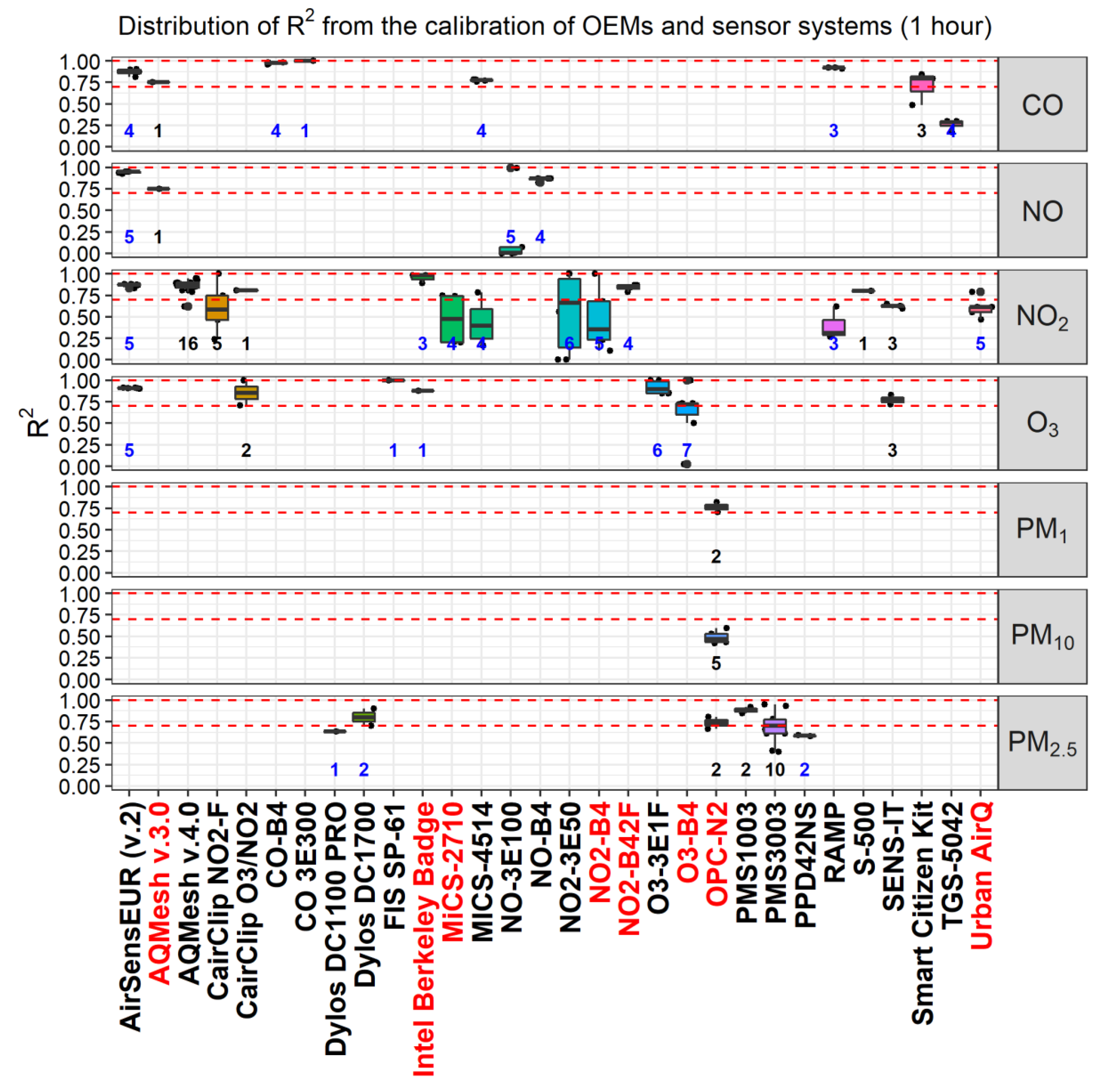
- For the measurement of PM2.5, values of R2 close to 1 were found for hourly data of PMS1003 and PMS3003 by Plantower [75] DC1100 PRO and DC1700 by Dylos (Riverside, USA) for minute data [14,19,79]. Strangely, higher R2 were reported for the Plantower and Dylos when calibrated with minute data than for hourly data. The OPC-N2 by AlphaSense [19] reported values of R2 falling within the range of 0.7–1.0. The same OPC-N2 reported values of R2 just above 0.7 when measuring PM1, while it did not show a good performance when measuring PM10 [19] (R2 less than 0.5). We need to stress that optical sensors, such as OPCs and nephelometers, are somewhat limited in coping with gravity effects when detecting coarse PM because of the low-efficiency of the sampling system. Most of the regression models used for the calibration of LCS used hourly data.
- For the calibration of O3 LCS, the highest values of R2 for hourly data was reported for FIS SP-61 by FIS (Osaka, Japan) and O3-3E1F [20] by CityTechnology (Figure A1) (Portsmouth., UK). On the other hand, for minute data, values of R2 close to 1 were found for AirSensEUR (V.2) [22] by LiberaIntentio (Malnate, IT), as well as for the S-500 [19] by Aeroqual (Figure A2) (Auckland, NZ). AirSensEUR used a built-in AlphaSense OX-A431 OEM. We want to point out that most of the MLR models used to calibrate O3 LCS need NO2 to correct for the strong NO2 cross-sensitivity.
- For the calibration of NO2 LCS, we found values of R2 for hourly data within the range of 0.7–1.0 for the NO2-B42F [59] (by Alphasense), for the AirSensEUR (v.2) [22] by LiberaIntentio, and for the minute values of MAS [40] (see Figure 3). The NO2 measurement by AirSensEUR (v.2) is carried out using the NO2-B43F OEM by AlphaSense.
- Most of the records of the calibration of CO LCS showed high values of R2. As shown in Figure A1, the OEMs CO 3E300 [23] by City Technology and CO-B4 [59] by Alphasense reported R2~1 for hourly data. High values of R2 were also reported for the SSys AirSensEUR (v.2) when calibrating CO minute data [22] (Figure A2). Other LCS reporting values of R2 within the range of 0.7–1.0 for hourly data consisted of the MICS-4515 [62] by SGX Sensortech (Corcelles-Cormondreche, CH), the Smart Citizen Kit [19] by Acrobotic (https://acrobatic.com), and RAMP [61].
4.2. Comparison of Calibrated Low-Cost Sensors with Reference Measurements
- For the SSys, PA-II by PurpleAir [19] and PATS + by Berkley Air [72] showed the highest R² with values between 0.8 and 1.0. Other LCS with R2 values ranging between 0.7 and 1.0 included PMS-SYS-1 by Shinyei (Kobe, JPN) , Dylos 1100 PRO by Dylos, MicroPEM by RTI (Research Triangle Park, USA), AirNUT by Moji (Beijing, CN), the Egg (2018) by Air Quality Egg (https://airqualityegg.com/home), AQT410 v.1.15 by Vaisala (Helsinki, Finland), AirVeraCity by AirVeraCity (Lausane, CH), NPM2 [33] by MetOne (Grants Pass, OR, USA), and the Air Quality Station [19] by AS LUNG. Nevertheless, we need to point out that the performance of LCS measuring PM10, on average, was very poor.
- For the hourly PM measurements of OEMs (Figure A5), the OPC-N2, OPC-N3 [19,35,36,49,84] and the SDS011 [49] by Nova Fitness (Jinan, CN) showed R2 values in the range of 0.7–1.0. For the 24-hour PM measurements of OEMs (Figure A6), we found R2 within the range of 0.7–1.0 for the OPC-N2 and the OPC-N3 [19].
- For the hourly gaseous measurements (Figure A5), we found very few OEMs with R2 in the range of 0.7–1.0. These included CairClip O3/NO2 [20,30,36,64] by CairPol (Poissy, France), Aeroqual Series 500 (and SM50) [33] and O3-3E1F [20,23,36] by CityTechnology, and NO2-B43F [61,65] by Alphasense. On the other hand, we found very few records for SSys using daily data. Additionally, one can notice when comparing Figure A4 and Figure A5 that the performance of OEMs is generally enhanced when they are integrated inside SSys, except for PM10.
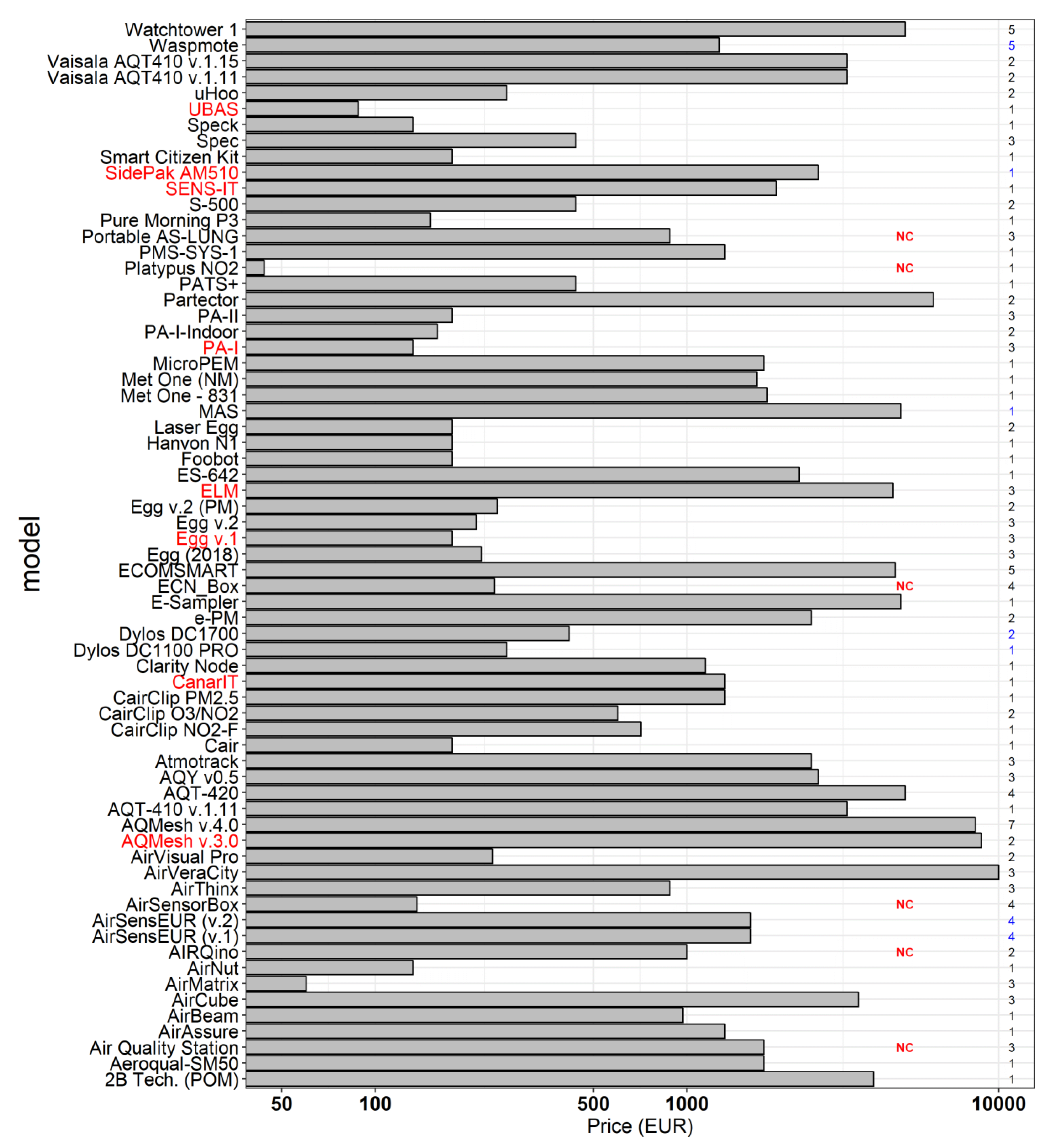
5. Cost of Purchase
6. Conclusions
Author Contributions
Funding
Acknowledgments
Conflicts of Interest
Appendix A

| Averaging Time | n. Records | n. OEMs and SSys |
|---|---|---|
| hourly | 610 | 86 |
| 5 min | 253 | 40 |
| daily | 248 | 42 |
| 1 min | 214 | 33 |
| Model | Pollutant | Type | Reference | Open/Close | Living | Price |
|---|---|---|---|---|---|---|
| CO-B4 | CO | electrochemical | Wei [59] | open source | N | 50 |
| CO 3E300 | CO | electrochemical | Gerboles [23] | open source | Y | 100 |
| DataRAM pDR-1200 | PM2.5 | nephelometer | Chakrabarti [70] | black box | N | - |
| DiscMini | PM | OPC | Viana [77] | open source | Y | 11,000 |
| DN7C3CA006 | PM2.5 | nephelometer | Sousan [83] | open source | Y | 10 |
| DSM501A | PM2.5 | nephelometer | Wang [68], Alvarado [69] | open source | Y | 15 |
| FIS SP-61 | O3 | MOs | Spinelle [26] | open source | Y | 50 |
| GP2Y1010AU0F | PM2.5, PM10 | nephelometer | Olivares [71], Manikonda [54], Sousan [83], Alvarado [69], Wang [68] | open source | Y | 10 |
| MiCS-2710 | NO2 | MOs | Spinelle [20], Williams [30] | open source | N | 7 |
| MICS-4514 | CO, NO2 | MOs | Spinelle [20,24] | open source | Y | 20 |
| NO-3E100 | NO | electrochemical | Spinelle [24], Gerboles [23] | open source | Y | 120 |
| NO-B4 | NO | electrochemical | Wei [59] | open source | Y | 50 |
| NO2-3E50 | NO2 | electrochemical | Spinelle [20], Gerboles [23] | open source | Y | 100 |
| NO2-A1 | NO2 | electrochemical | Williams [30] | black box | Y | 50 |
| NO2-B4 | NO2 | electrochemical | Spinelle [20,25] | open source | N | 50 |
| NO2-B42F | NO2 | electrochemical | Wei [59] | open source | N | 50 |
| NO2-B43F | NO2 | electrochemical | Sun [65] | open source | Y | 50 |
| O3-B4 | O3 | electrochemical | Spinelle [20,25], Wei [59] | open source | N | 50 |
| O3-3E1F | O3 | electrochemical | Spinelle [20,25], Gerboles [23] | open source | Y | 500 |
| OPC-N2 | PM1, PM2.5 | OPC | AQ-SPEC [19], Mukherjee [35], Sousan [83], Feinberg [36], Crilley [84], Badura [49], Crunaire [33] | open source, black box | N | 362 |
| OPC-N3 | PM1, PM2.5 | OPC | AQ-SPEC [19] | open source | Y | 338 |
| PMS1003 | PM2.5 | OPC | Kelly [75] | black box | Y | 20 |
| PMS3003 | PM2.5 | OPC | Zheng [85], Kelly [75] | open source, black box | Y | 30 |
| PMS5003 | PM2.5 | OPC | Laquai [48] | black box | Y | 15 |
| PMS7003 | PM2.5 | OPC | Badura [49] | black box | Y | 20 |
| PPD42NS | PM2.5, PM3, PM2 | nephelometer | Wang [68], Holstius [51], Austin [73], Gao [74], Kelly [75] | open source | Y | 15 |
| SDS011 | PM2.5, | OPC | Budde [47], Laquai [48], Badura [49], Liu [52] | open source | Y | 30 |
| SM50 | O3 | MOs | Feinberg [36] | open source | Y | 500 |
| TGS-5042 | CO | MOs | Spinelle [24] | open source | Y | 40 |
| TZOA-PM Research Sensors | PM | nephelometer | Feinberg [36] | open source | Y | 90 |
| ZH03A | PM2.5 | nephelometer | Badura [49] | black box | Y | 20 |
| Model | Pollutant | Type | Reference | Open/Close | Living | Price |
|---|---|---|---|---|---|---|
| 2B Tech. (POM) | O3 | UV | AQ-SPEC [19] | black box | Y | 4500 |
| Aeroqual-SM50 | O3 | MOs | Jiao [39] | black box | Y | 2000 |
| AGT ATS-35 NO2 | NO2 | MOs | Williams [30] | black box | N | -d |
| Air Quality Station | PM1, PM2.5 | OPC | AQ-SPEC [19] | black box | Y | 2000 |
| AirAssure | PM2.5 | nephelometer | AQ-SPEC [19], Feinberg [36], Manikonda [54] | black box | Y | 1500 |
| AirBeam | PM2.5 | OPC, nephelometer | AQ-SPEC [19], Mukherjee [35], Feinberg [36], Borghi [37], Jiao [39], Crunaire [33] | black box | Y | 200 |
| AirCube | NO2, O3, NO | electrochemical | Mueller [43], Bigi [42] | black box | Y | 3538 |
| AirMatrix | PM1, PM2.5 | nephelometer | Crunaire [33] | black box | Y | 60 |
| AirNut | PM2.5 | nephelometer | AQ-SPEC [19] | black box | Y | 150 |
| AIRQino | PM2.5 | OPC | Cavaliere [76] | open source | Y | 1000 |
| AirSensEUR (v.1) | NO, NO2, O3 | electrochemical | Crunaire [33] | black box | Y | 1600 |
| AirSensEUR (v.2) | CO, NO, NO2, O3 | electrochemical | Karagulian [22] | open source | Y | 1600 |
| AirSensorBox | NO2, CO, O3 | electrochemical, MOs, nephelometer | Borrego [53] | black box | Y | 280 |
| AirThinx | PM1, PM2.5 | OPC | AQ-SPEC [19] | black box | Y | 1000 |
| AirVeraCity | CO, NO2, O3 | electrochemical, MOs | Marjovi [57] | black box | Y | 10000 |
| AirVisual Pro | PM2.5 | nephelometer | AQ-SPEC [19] | black box | Y | 270 |
| AQMesh v.3.0 | CO, NO | electrochemical | Jiao [39] | black box | N | 10000 |
| AQMesh v.4.0 | NO2, CO, NO, O3 | electrochemical | Cordero [63], AQ-SPEC [19], Castell [10], Borrego [53], Crunaire [33] | black box | updated | 10000 |
| AQT410 v.1.11 | O3 | electrochemical | AQ-SPEC [19] | black box | Y | 3700 |
| AQT-420 | NO2,O3, PM2.5 | electrochemical, OPC | Crunaire [33] | black box | Y | 3256 |
| AQY v0.5 | PM2.5, NO2, O3 | OPC, electrochemical, MOs | AQ-SPEC [19] | black box | updated | 3000 |
| ARISense | NO2, CO, NO, O3 | electrochemical | Cross [58] | black box | Y | - |
| Atmotrack | PM1, PM2.5 | nephelometer | Crunaire [33] | black box | Y | 2500 |
| BAIRS | PM2.5–0.5 | OPC | Northcross [78] | open source | N | 475 |
| Cair | PM2.5, PM10–2.5 | OPC | AQ-SPEC [19] | black box | Y | 200 |
| CairClip O3/NO2 | O3, NO2 | electrochemical | Jiao [39], Spinelle [25], Williams [30], Duvall [64], Feinberg [36] | black box | Y | 600 |
| CairClip NO2-F | NO2 | electrochemical | Spinelle [20], Duvall [64], Crunaire [33] | black box | Y | 600 |
| CairClip PM2.5 | PM2.5 | nephelometer | Williams [31] | black box | Y | 1500 |
| CAM | PM10, PM2.5, NO2, CO, NO | OPC, electrochemical | Borrego [53] | black box | Y | - |
| CanarIT | PM | nephelometer | Williams [31] | black box | N | 1500 |
| Clarity Node | PM2.5 | nephelometer | AQ-SPEC [19] | black box | Y | 1300 |
| Dylos DC1100 | PM2.5–0.5 | OPC | Jiao [39], Williams [31], Feinberg [36] | black box, open source | Y | 300 |
| Dylos DC1100 PRO | PM2.5–0, PM10–2.5, PM10 | OPC | Jiao [39], AQ-SPEC [19], Feinberg [36], Manikonda [54] | black box, open source | Y | 300 |
| Dylos DC1700 | PM2.5–0.5, PM10, PM10–2.5, PM3, PM2, PM2.5 | OPC | Manikonda [54], Sousan [83], Northcross [78], Holstius [51], Steinle [79], Han [80], Jovasevic [81], Dacunto [82] | open source | Y | 475 |
| e-PM | PM10, PM2.5 | nephelometer | Crunaire [33] | black box | Y | 2500 |
| E-Sampler | PM2.5 | OPC | AQ-SPEC [19] | black box | Y | 5500 |
| ECN_Box | PM10, PM2.5, NO2, O3 | nephelometer, electrochemical | Borrego [53] | black box | Y | 274 |
| Eco PM | PM1 | OPC | Williams [31] | black box | N | |
| ECOMSMART | NO2, O3, PM1, PM10, PM2.5 | electrochemical, OPC | Crunaire [33] | black box | Y | 4560 |
| Egg (2018) | PM1, PM2.5, PM10 | OPC | AQ-SPEC [19] | black box | Y | 249 |
| Egg v.1 | CO, NO2, O3 | MOs | AQ-SPEC [19] | black box | N | 200 |
| Egg v.2 | CO, NO2, O3 | electrochemical | AQ-SPEC [19] | black box | Y | 240 |
| Egg v.2 (PM) | PM2.5, PM10 | nephelometer | AQ-SPEC [19] | black box | Y | 280 |
| ELM | NO2, PM10, O3 | MOs, nephelometer | AQ-SPEC [19], US-EPA [67] | black box | N | 5200 |
| EMMA | PM2.5, CO, NO2, NO | OPC, electrochemical | Gillooly [60] | black box | Y | - |
| ES-642 | PM2.5 | OPC | Crunaire [33] | black box | Y | 2600 |
| Foobot | PM2.5 | OPC | AQ-SPEC [19] | black box | Y | 200 |
| Hanvon N1 | PM2.5 | nephelometer | AQ-SPEC [19] | black box | Y | 200 |
| Intel Berkeley Badge | NO2, O3 | electrochemical, MOs | Vaughn [32] | open source | N | - |
| ISAG | NO2, O3 | MOs | Borrego [53] | black box | N | - |
| Laser Egg | PM2.5, PM10 | nephelometer | AQ-SPEC [19] | black box | Y | 200 |
| M-POD | CO, NO2 | MOs | Piedrahita [62] | black box | N | |
| MAS | CO, NO2, O3, PM2.5 | electrochemical, UV, nephelometer | Sun [40] | black box, open source | N, Y | 5500 |
| Met One-831 | PM10 | OPC | Williams [31] | black box | Y | 2050 |
| Met One (NM) | PM2.5 | OPC | AQ-SPEC [19] | black box | Y | 1900 |
| MicroPEM | PM2.5 | nephelometer | AQ-SPEC [19], Williams [31] | black box | Y | 2000 |
| NanoEnvi | NO2, O3, CO | electrochemical, MOs | Borrego [53] | black box | Y | - |
| PA-I | PM1, PM2.5, PM10 | OPC | AQ-SPEC [19] | black box | N | 150 |
| PA-I-Indoor | PM2.5, PM10 | OPC | AQ-SPEC [19] | black box | Y | 180 |
| PA-II | PM1, PM2.5, PM10 | OPC | AQ-SPEC [19] | black box | Y | 200 |
| Partector | PM1, PM2.5 | Electrical | AQ-SPEC [19] | black box | Y | 7000 |
| PATS+ | PM2.5 | nephelometer | Pillarisetti [72] | black box | Y | 500 |
| Platypus NO2 | NO2 | MOs | Williams [30] | black box | Y | 50 |
| PMS-SYS-1 | PM2.5 | nephelometer | Jiao [39], AQ-SPEC [19], Williams [31], Feinberg [36] | black box | Y | 1000 |
| Portable AS-LUNG | PM1, PM2.5, PM10 | OPC | AQ-SPEC [19] | black box | Y | 1000 |
| Pure Morning P3 | PM2.5 | OPC | AQ-SPEC [19] | black box | Y | 170 |
| RAMP | CO, NO2 | electrochemical | Zimmerman [61] | open source | Y | - |
| S-500 | NO2, O3 | MOs | Lin [66], AQ-SPEC [19], Vaughn [32] | black box | Y | 500 |
| SENS-IT | O3, CO, NO2 | MOs | AQ-SPEC [19] | black box | N, Y | 2200 |
| SidePak AM510 | PM2.5 | nephelometer | Karagulian [28] | open source | Y | 3000 |
| Smart Citizen Kit | CO | MOs | AQ-SPEC [19] | black box | Y | 200 |
| SNAQ | NO2, CO, NO | electrochemical | Mead [44], Popoola [45] | black box | Y | - |
| Spec | CO, NO2, O3 | electrochemical | AQ-SPEC [19] | black box | Y | 500 |
| Speck | PM2.5 | nephelometer | Feinberg [36], US-EPA [67], Williams [31], AQ-SPEC [19], Manikonda [54], Zikova [55] | black box | Y | 150 |
| UBAS | PM2.5 | nephelometer | Manikonda [54] | black box | N | 100 |
| uHoo | PM2.5, O3 | nephelometer, MOs | AQ-SPEC [19] | black box | Y | 300 |
| Urban AirQ | NO2 | electrochemical | Mijling [41] | open source | N | - |
| Vaisala AQT410 v.1.11 | CO, NO2 | electrochemical | AQ-SPEC [19] | black box | Y | 3700 |
| Vaisala AQT410 v.1.15 | CO, NO2 | electrochemical | AQ-SPEC [19] | black box | Y | 3700 |
| Waspmote | NO, NO2, PM1, PM10, PM2.5 | MOs, OPC | Crunaire [33] | black box | Y | 1270 |
| Watchtower 1 | NO2, PM1, PM10, PM2.5, O3 | electrochemical, OPC | Crunaire [33] | black box | Y | 5000 |


| Model | Pollutant | Mean | Mean Slope | Mean Absolute Intercept | Open/Close | Living | Commercial | Price (EUR) |
|---|---|---|---|---|---|---|---|---|
| PA-I | PM1 | 0.99 | 0.9 | 0.47 | black box | N | commercial | 132 |
| PA-II | PM1 | 0.99 | 0.8 | 1.8 | black box | Y | commercial | 176 |
| Egg (2018) | PM1 | 0.88 | 0.8 | 0.33 | black box | Y | commercial | 219 |
| Egg v.2 (PM) | PM2.5 | 0.94 | 1 | 3.3 | black box | Y | commercial | 246 |
| AirThinx | PM1 | 0.89 | 0.8 | 1.3 | black box | Y | commercial | 880 |
| Portable AS-LUNG | PM1 | 0.93 | 0.9 | 1.5 | black box | Y | non-commercial | 880 |
| AIRQino | PM2.5, PM10 | 0.91 | 1 | 1.1 | open source | Y | non-commercial | 1000 |
| Air Quality Station | PM1 | 0.94 | 0.9 | 1.1 | black box | Y | non-commercial | 1760 |
| AQY v0.5 | PM2.5 | 0.91 | 0.9 | 4.0 | black box | updated | commercial | 2640 |
| Vaisala AQT410 v.1.15 | CO | 0.86 | 0.9 | 0.25 | black box | Y | commercial | 3256 |
References
- Kumar, P.; Morawska, L.; Martani, C.; Biskos, G.; Neophytou, M.; Di Sabatino, S.; Bell, M.; Norford, L.; Britter, R. The rise of low-cost sensing for managing air pollution in cities. Environ. Int. 2015, 75, 199–205. [Google Scholar] [CrossRef] [PubMed] [Green Version]
- 2008/50/EC: Directive of the European Parliament and of the Council of 21 May 2008 on ambient air quality and cleaner air for Europe. Available online: http://eurlex.europa.eu/Result.do?RechType=RECH_celex&lang=en&code=32008L0050 (accessed on 22 August 2019).
- CEN. Ambient Air—Standard Gravimetric Measurement Method for the Determination of the PM10 or PM2,5 Mass Concentration of Suspended Particulate Matter (EN 12341:2014); European Committee for Standardization: Brussels, Belgium, 2014. [Google Scholar]
- CEN Ambient Air. Standard Method for the Measurement of the Concentration of Carbon Monoxide by Non-Dispersive Infrared Spectroscopy, (EN 14626:2012); European Committee for Standardization: Brussels, Belgium, 2012. [Google Scholar]
- CEN Ambient Air. Standard Method for the Measurement of the Concentration of Nitrogen Dioxide and Nitrogen Monoxide by Chemiluminescence (EN 14211:2012); European Committee for Standardization: Brussels, Belgium, 2012. [Google Scholar]
- CEN Ambient Air. Standard Method for the Measurement of the Concentration of Ozone by Ultraviolet Photometry (EN 14625:2012); European Committee for Standardization: Brussels, Belgium, 2012. [Google Scholar]
- CEN Ambient Air. Standard Method for the Measurement of the Concentration of Sulphur Dioxide by Ultraviolet Fluorescence, (EN 14212:2012); European Committee for Standardization: Brussels, Belgium, 2012. [Google Scholar]
- Lewis, A.C.; von Schneidemesser, E.; Peltier, R. Low-cost sensors for the measurement of atmospheric composition: overview of topic and future applications (World Meteorological Organization). Available online: https://www.ccacoalition.org/en/resources/low-cost-sensors-measurement-atmospheric-composition-overview-topic-and-future (accessed on 21 August 2019).
- Aleixandre, M.; Gerboles, M. Review of small commercial sensors for indicative monitoring of ambient gas. Chem. Eng. Trans. 2012, 30, 169–174. [Google Scholar]
- Castell, N.; Dauge, F.R.; Schneider, P.; Vogt, M.; Lerner, U.; Fishbain, B.; Broday, D.; Bartonova, A. Can commercial low-cost sensor platforms contribute to air quality monitoring and exposure estimates? Environ. Int. 2017, 99, 293–302. [Google Scholar] [CrossRef] [PubMed]
- iScape. Summary of Air Quality sensors and recommendations for application. Available online: https://www.iscapeproject.eu/wp-content/uploads/2017/09/iSCAPE_D1.5_Summary-of-air-quality-sensors-and-recommendations-for-application.pdf (accessed on 21 August 2019).
- Snyder, E.G.; Watkins, T.H.; Solomon, P.A.; Thoma, E.D.; Williams, R.W.; Hagler, G.S.W.; Shelow, D.; Hindin, D.A.; Kilaru, V.J.; Preuss, P.W. The changing paradigm of air pollution monitoring. Environ. Sci. Technol. 2013, 47, 11369–11377. [Google Scholar] [CrossRef] [PubMed]
- White, R.M.; Paprotny, I.; Doering, F.; Cascio, W.E.; Solomon, P.A.; Gundel, L.A. Sensors and “apps” for community-based: Atmospheric monitoring. EM Air Waste Manag. Assoc. Mag. Environ. Manag. 2012, 5, 36–40. [Google Scholar]
- Williams, R.; Kilaru, V.; Snyder, E.; Kaufman, A.; Dye, T.; Rutter, A.; Russell, A.; Hafner, H. Air Sensor Guidebook; United States Environmental Protection Agency (US-EPA): Washington, DC, USA, 2014. [Google Scholar]
- Zhou, X.; Lee, S.; Xu, Z.; Yoon, J. Recent Progress on the Development of Chemosensors for Gases. Chem. Rev. 2015, 115, 7944–8000. [Google Scholar] [CrossRef] [PubMed]
- Spinelle, L.; Aleixandre, M.; Gerboles, M. Protocol of Evaluation and Calibration of Low-Cost Gas Sensors for the Monitoring of Air Pollution; Publications Office of the European Union: Luxembourg, 2013. [Google Scholar]
- Redon, N.; Delcourt, F.; Crunaire, S.; Locoge, N. Protocole de détermination des caractéristiques de performance métrologique des micro-capteurs-étude comparative des performances en laboratoire de micro-capteurs de NO2 | LCSQA. Available online: https://www.lcsqa.org/fr/rapport/2016/mines-douai/protocole-determination-caracteristiques-performance-metrologique-micro-cap (accessed on 22 August 2019).
- Williams, R.; Duvall, R.; Kilaru, V.; Hagler, G.; Hassinger, L.; Benedict, K.; Rice, J.; Kaufman, A.; Judge, R.; Pierce, G.; et al. Deliberating performance targets workshop: Potential paths for emerging PM2.5 and O3 air sensor progress. Atmos. Environ. X 2019, 2, 100031. [Google Scholar] [CrossRef]
- AQ-SPEC; South Coast Air Quality Management District; South Coast Air Quality Management District Air Quality Sensor Performance Evaluation Reports. Available online: http://www.aqmd.gov/aq-spec/evaluations#&MainContent_C001_Col00=2 (accessed on 29 December 2015).
- Spinelle, L.; Gerboles, M.; Villani, M.G.; Aleixandre, M.; Bonavitacola, F. Field calibration of a cluster of low-cost available sensors for air quality monitoring. Part A: Ozone and nitrogen dioxide. Sens. Actuators B Chem. 2015, 215, 249–257. [Google Scholar] [CrossRef]
- Lewis, A.; Edwards, P. Validate personal air-pollution sensors. Nat. News 2016, 535, 29. [Google Scholar] [CrossRef]
- Karagulian, F.; Borowiak, A.; Barbiere, M.; Kotsev, A.; van der Broecke, J.; Vonk, J.; Signorini, M.; Gerboles, M. Calibration of AirSensEUR Units during a Field Study in the Netherlands; European Commission-Joint Research Centre: Ispra, Italy, 2019; in press. [Google Scholar]
- Gerboles, M.; Spinelle, L.; Signorini, M. AirSensEUR: An Open Data/Software/Hardware Multi-Sensor Platform for Air Quality Monitoring. Part A: Sensor Shield; Publications Office of the European Union: Luxembourg, 2015. [Google Scholar]
- Spinelle, L.; Gerboles, M.; Villani, M.G.; Aleixandre, M.; Bonavitacola, F. Field calibration of a cluster of low-cost commercially available sensors for air quality monitoring. Part B: NO, CO and CO2. Sens. Actuators B Chem. 2017, 238, 706–715. [Google Scholar] [CrossRef]
- Spinelle, L.; Gerboles, M.; Aleixandre, M. Performance Evaluation of Amperometric Sensors for the Monitoring of O 3 and NO 2 in Ambient Air at ppb Level. Procedia Eng. 2015, 120, 480–483. [Google Scholar] [CrossRef]
- Spinelle, L.; Gerboles, M.; Aleixandre, M.; Bonavitacola, F. Evaluation of metal oxides sensors for the monitoring of O3 in ambient air at ppb level. Chem. Eng. Trans. 2016, 319–324. [Google Scholar]
- Spinelle, L.; Gerboles, M.; Kotsev, A.; Signorini, M. Evaluation of Low-Cost Sensors for Air Pollution Monitoring: Effect of Gaseous Interfering Compounds and Meteorological Conditions; Publications Office of the European Union: Luxembourg, 2017. [Google Scholar]
- Karagulian, F.; Belis, C.A.; Lagler, F.; Barbiere, M.; Gerboles, M. Evaluation of a portable nephelometer against the Tapered Element Oscillating Microbalance method for monitoring PM2.5. J. Env. Monit. 2012, 14, 2145–2153. [Google Scholar] [CrossRef] [PubMed]
- US-EPA. Air Sensor Toolbox; Evaluation of Emerging Air Pollution Sensor Performance. US-EPA. Available online: https://www.epa.gov/air-sensor-toolbox/evaluation-emerging-air-pollution-sensor-performance (accessed on 21 August 2018).
- Williams, R.; Long, R.; Beaver, M.; Kaufman, A.; Zeiger, F.; Heimbinder, M.; Acharya, B.R.; Grinwald, B.A.; Kupcho, K.A.; Tobinson, S.E. Sensor Evaluation Report; U.S. Environmental Protection Agency: Washington, DC, USA, 2014. [Google Scholar]
- Williams, R.; Kaufman, A.; Hanley, T.; Rice, J.; Garvey, S. Evaluation of Field-deployed Low Cost PM Sensors; U.S. Environmental Protection Agency: Washington, DC, USA, 2014. [Google Scholar]
- Vaughn, D.L.; Dye, T.S.; Roberts, P.T.; Ray, A.E.; DeWinter, J.L. Characterization of low-Cost NO2 Sensors; U.S. Environmental Protection Agency: Washington, DC, USA, 2010. [Google Scholar]
- Crunaire, S.; Redon, N.; Spinelle, L. 1ER Essai national d’Aptitude des Microcapteurs EAμC) pour la Surveillance de la Qualité de l’Air: Synthèse des Résultas; LCSQA: Paris, France, 2018; p. 38. [Google Scholar]
- Fishbain, B.; Lerner, U.; Castell, N.; Cole-Hunter, T.; Popoola, O.; Broday, D.M.; Iñiguez, T.M.; Nieuwenhuijsen, M.; Jovasevic-Stojanovic, M.; Topalovic, D.; et al. An evaluation tool kit of air quality micro-sensing units. Sci. Total Environ. 2017, 575, 639–648. [Google Scholar] [CrossRef] [PubMed]
- Mukherjee, A.; Stanton, L.G.; Graham, A.R.; Roberts, P.T. Assessing the Utility of Low-Cost Particulate Matter Sensors over a 12-Week Period in the Cuyama Valley of California. Sensors 2017, 17, 1805. [Google Scholar] [CrossRef] [PubMed]
- Feinberg, S.; Williams, R.; Hagler, G.S.W.; Rickard, J.; Brown, R.; Garver, D.; Harshfield, G.; Stauffer, P.; Mattson, E.; Judge, R.; et al. Long-term evaluation of air sensor technology under ambient conditions in Denver, Colorado. Atmos. Meas. Tech. 2018, 11, 4605–4615. [Google Scholar] [CrossRef] [Green Version]
- Borghi, F.; Spinazzè, A.; Campagnolo, D.; Rovelli, S.; Cattaneo, A.; Cavallo, D.M. Precision and Accuracy of a Direct-Reading Miniaturized Monitor in PM2.5 Exposure Assessment. Sensors 2018, 18, 3089. [Google Scholar] [CrossRef]
- Zikova, N.; Masiol, M.; Chalupa, D.C.; Rich, D.Q.; Ferro, A.R.; Hopke, P.K. Estimating Hourly Concentrations of PM2.5 across a Metropolitan Area Using Low-Cost Particle Monitors. Sensor (Basel) 2017, 17, 1992. [Google Scholar] [CrossRef]
- Jiao, W.; Hagler, G.; Williams, R.; Sharpe, R.; Brown, R.; Garver, D.; Judge, R.; Caudill, M.; Rickard, J.; Davis, M.; et al. Community Air Sensor Network (CAIRSENSE) project: evaluation of low-cost sensor performance in a suburban environment in the southeastern United States. Atmos. Meas. Tech. 2016, 9, 5281–5292. [Google Scholar] [CrossRef] [Green Version]
- Sun, L.; Wong, K.C.; Wei, P.; Ye, S.; Huang, H.; Yang, F.; Westerdahl, D.; Louie, P.K.K.; Luk, C.W.Y.; Ning, Z. Development and Application of a Next Generation Air Sensor Network for the Hong Kong Marathon 2015 Air Quality Monitoring. Sensor (Basel) 2017, 17, 1922. [Google Scholar] [CrossRef]
- Mijling, B.; Jiang, Q.; de Jonge, D.; Bocconi, S. Practical field calibration of electrochemical NO2 sensors for urban air quality applications. Atmos. Meas. Tech. Discuss. 2017, 2017, 1–25. [Google Scholar] [CrossRef]
- Bigi, A.; Mueller, M.; Grange, S.K.; Ghermandi, G.; Hueglin, C. Performance of NO, NO2 low cost sensors and three calibration approaches within a real world application. Atmos. Meas. Tech. 2018, 11, 3717–3735. [Google Scholar] [CrossRef]
- Mueller, M.; Meyer, J.; Hueglin, C. Design of an ozone and nitrogen dioxide sensor unit and its long-term operation within a sensor network in the city of Zurich. Atmos. Meas. Tech. 2017, 10, 3783–3799. [Google Scholar] [CrossRef] [Green Version]
- Mead, M.I.; Popoola, O.A.M.; Stewart, G.B.; Landshoff, P.; Calleja, M.; Hayes, M.; Baldovi, J.J.; McLeod, M.W.; Hodgson, T.F.; Dicks, J.; et al. The use of electrochemical sensors for monitoring urban air quality in low-cost, high-density networks. Atmos. Environ. 2013, 70, 186–203. [Google Scholar] [CrossRef] [Green Version]
- Popoola, O.A.M.; Stewart, G.B.; Mead, M.I.; Jones, R.L. Development of a baseline-temperature correction methodology for electrochemical sensors and its implications for long-term stability. Atmos. Environ. 2016, 147, 330–343. [Google Scholar] [CrossRef] [Green Version]
- Mooney, D.; Willis, P.; Stevenson, K. A Guide for Local Authorities Purchasing Air Quality Monitoring Equipment. Available online: https://uk-air.defra.gov.uk/library/reports?report_id=386 (accessed on 21 August 2019).
- Budde, M.; Müller, T.; Laquai, B.; Streibl, N.; Schwarz, A.; Schindler, G.; Riedel, T.; Beigl, M.; Dittler, A. Suitability of the Low-Cost SDS011 Particle Sensor for Urban PM-Monitoring. In Proceedings of the 3rd International Conference on Atmospheric Dust, Bari, Italy, 29–31 May 2018. [Google Scholar]
- Laquai, B. Particle Distribution Dependent Inaccuracy of the Plantower PMS5003 low-cost PM-sensor. Available online: https://www.researchgate.net/publication/320555036 (accessed on 21 August 2019).
- Budde, M.; Müller, T.; Laquai, B.; Streibl, N.; Schwarz, A.; Schindler, G.; Riedel, T.; Beigl, M.; Dittler, A. Optical particulate matter sensors in PM2.5 measurements in atmospheric air. E3S Web Conf. 2018, 44, 00006. [Google Scholar]
- The World Air Quality Index. Sensing the Air Quality: Research on Air Quality Sensors. Available online: http://aqicn.org/sensor/ (accessed on 21 August 2019).
- Holstius, D.M.; Pillarisetti, A.; Smith, K.R.; Seto, E. Field calibrations of a low-cost aerosol sensor at a regulatory monitoring site in California. Atmos. Meas. Tech. 2014, 7, 1121–1131. [Google Scholar] [CrossRef] [Green Version]
- Liu, H.-Y.; Schneider, P.; Haugen, R.; Vogt, M. Performance Assessment of a Low-Cost PM2.5 Sensor for a near Four-Month Period in Oslo, Norway. Atmosphere 2019, 10, 41. [Google Scholar] [CrossRef]
- Borrego, C.; Costa, A.M.; Ginja, J.; Amorim, M.; Coutinho, M.; Karatzas, K.; Sioumis, Th.; Katsifarakis, N.; Konstantinidis, K.; De Vito, S.; et al. Assessment of air quality microsensors versus reference methods: The EuNetAir joint exercise. Atmos. Environ. 2016, 147, 246–263. [Google Scholar] [CrossRef] [Green Version]
- Manikonda, A.; Zíková, N.; Hopke, P.K.; Ferro, A.R. Laboratory assessment of low-cost PM monitors. J. Aerosol Sci. 2016, 102, 29–40. [Google Scholar] [CrossRef]
- Zikova, N.; Hopke, P.K.; Ferro, A.R. Evaluation of new low-cost particle monitors for PM2.5 concentrations measurements. J. Aerosol Sci. 2017, 105, 24–34. [Google Scholar] [CrossRef]
- Sousan, S.; Koehler, K.; Hallett, L.; Peters, T.M. Evaluation of the Alphasense optical particle counter (OPC-N2) and the Grimm portable aerosol spectrometer (PAS-1.108). Aerosol Sci. Technol. 2016, 50, 1352–1365. [Google Scholar] [CrossRef] [PubMed]
- Marjovi, A.; Arfire, A.; Martinoli, A. Extending Urban Air Quality Maps Beyond the Coverage of a Mobile Sensor Network: Data Sources, Methods, and Performance Evaluation. In Proceedings of the 2017 International Conference on Embedded Wireless Systems and Networks, Uppsala, Sweden, 20–22 February 2017; pp. 12–23. [Google Scholar]
- Cross, E.S.; Williams, L.R.; Lewis, D.K.; Magoon, G.R.; Onasch, T.B.; Kaminsky, M.L.; Worsnop, D.R.; Jayne, J.T. Use of electrochemical sensors for measurement of air pollution: correcting interference response and validating measurements. Atmos. Meas. Tech. 2017, 10, 3575–3588. [Google Scholar] [CrossRef] [Green Version]
- Wei, P.; Ning, Z.; Ye, S.; Sun, L.; Yang, F.; Wong, K.; Westerdahl, D.; Louie, P. Impact Analysis of Temperature and Humidity Conditions on Electrochemical Sensor Response in Ambient Air Quality Monitoring. Sensors 2018, 18, 59. [Google Scholar] [CrossRef] [PubMed]
- Gillooly, S.E.; Zhou, Y.; Vallarino, J.; Chu, M.T.; Michanowicz, D.R.; Levy, J.I.; Adamkiewicz, G. Development of an in-home, real-time air pollutant sensor platform and implications for community use. Environ. Pollut. 2019, 244, 440–450. [Google Scholar] [CrossRef]
- Zimmerman, N.; Presto, A.A.; Kumar, S.P.N.; Gu, J.; Hauryliuk, A.; Robinson, E.S.; Robinson, A.L.; Subramanian, R. A machine learning calibration model using random forests to improve sensor performance for lower-cost air quality monitoring. Atmos. Meas. Tech. 2018, 11, 291–313. [Google Scholar] [CrossRef] [Green Version]
- Piedrahita, R.; Xiang, Y.; Masson, N.; Ortega, J.; Collier, A.; Jiang, Y.; Li, K.; Dick, R.P.; Lv, Q.; Hannigan, M.; et al. The next generation of low-cost personal air quality sensors for quantitative exposure monitoring. Atmos. Meas. Tech 2014, 7, 3325–3336. [Google Scholar] [CrossRef] [Green Version]
- Cordero, J.M.; Borge, R.; Narros, A. Using statistical methods to carry out in field calibrations of low cost air quality sensors. Sens. Actuators B Chem. 2018, 267, 245–254. [Google Scholar] [CrossRef]
- Duvall, R.M.; Long, R.W.; Beaver, M.R.; Kronmiller, K.G.; Wheeler, M.L.; Szykman, J.J. Performance Evaluation and Community Application of Low-Cost Sensors for Ozone and Nitrogen Dioxide. Sensors 2016, 16, 1698. [Google Scholar] [CrossRef]
- Sun, L.; Westerdahl, D.; Ning, Z. Development and Evaluation of A Novel and Cost-Effective Approach for Low-Cost NO2 Sensor Drift Correction. Sensors 2017, 17, 1916. [Google Scholar] [CrossRef]
- Lin, C.; Gillespie, J.; Schuder, M.D.; Duberstein, W.; Beverland, I.J.; Heal, M.R. Evaluation and calibration of Aeroqual series 500 portable gas sensors for accurate measurement of ambient ozone and nitrogen dioxide. Atmos. Environ. 2015, 100, 111–116. [Google Scholar] [CrossRef]
- US-EPA. Evaluation of Elm and Speck Sensors. Available online: https://cfpub.epa.gov/si/si_public_record_report.cfm?Lab=NERL&dirEntryId=310285 (accessed on 21 August 2019).
- Wang, Y.; Li, J.; Jing, H.; Zhang, Q.; Jiang, J.; Biswas, P. Laboratory Evaluation and Calibration of Three Low-Cost Particle Sensors for Particulate Matter Measurement. Aerosol Sci. Technol. 2015, 49, 1063–1077. [Google Scholar] [CrossRef]
- Alvarado, M.; Gonzalez, F.; Fletcher, A.; Doshi, A.; Alvarado, M.; Gonzalez, F.; Fletcher, A.; Doshi, A. Towards the Development of a Low Cost Airborne Sensing System to Monitor Dust Particles after Blasting at Open-Pit Mine Sites. Sensors 2015, 15, 19667–19687. [Google Scholar] [CrossRef] [PubMed] [Green Version]
- Chakrabarti, B.; Fine, P.M.; Delfino, R.; Sioutas, C. Performance evaluation of the active-flow personal DataRAM PM2.5 mass monitor (Thermo Anderson pDR-1200) designed for continuous personal exposure measurements. Atmos. Environ. 2004, 38, 3329–3340. [Google Scholar] [CrossRef]
- Olivares, G.; Edwards, S. The Outdoor Dust Information Node (ODIN) – development and performance assessment of a low cost ambient dust sensor. Atmos. Meas. Tech. Discuss. 2015, 8, 7511–7533. [Google Scholar] [CrossRef]
- Pillarisetti, A.; Allen, T.; Ruiz-Mercado, I.; Edwards, R.; Chowdhury, Z.; Garland, C.; Hill, L.D.; Johnson, M.; Litton, C.D.; Lam, N.L.; et al. Small, Smart, Fast, and Cheap: Microchip-Based Sensors to Estimate Air Pollution Exposures in Rural Households. Sensor. (Basel) 2017, 17, 1879. [Google Scholar] [CrossRef] [PubMed]
- Austin, E.; Novosselov, I.; Seto, E.; Yost, M.G. Laboratory Evaluation of the Shinyei PPD42NS Low-Cost Particulate Matter Sensor. Plos ONE 2015, 10, e0137789. [Google Scholar]
- Gao, M.; Cao, J.; Seto, E. A distributed network of low-cost continuous reading sensors to measure spatiotemporal variations of PM2.5 in Xi’an, China. Environ. Pollut. 2015, 199, 56–65. [Google Scholar] [CrossRef] [PubMed]
- Kelly, K.E.; Whitaker, J.; Petty, A.; Widmer, C.; Dybwad, A.; Sleeth, D.; Martin, R.; Butterfield, A. Ambient and laboratory evaluation of a low-cost particulate matter sensor. Environ. Pollut. 2017, 221, 491–500. [Google Scholar] [CrossRef]
- Cavaliere, A.; Carotenuto, F.; Di Gennaro, F.; Gioli, B.; Gualtieri, G.; Martelli, F.; Matese, A.; Toscano, P.; Vagnoli, C.; Zaldei, A. Development of Low-Cost Air Quality Stations for Next Generation Monitoring Networks: Calibration and Validation of PM2.5 and PM10 Sensors. Sensors 2018, 18, 2843. [Google Scholar] [CrossRef]
- Viana, M.; Rivas, I.; Reche, C.; Fonseca, A.S.; Pérez, N.; Querol, X.; Alastuey, A.; Álvarez-Pedrerol, M.; Sunyer, J. Field comparison of portable and stationary instruments for outdoor urban air exposure assessments. Atmos. Environ. 2015, 123 Pt A, 220–228. [Google Scholar] [CrossRef]
- Northcross, A.L.; Edwards, R.J.; Johnson, M.A.; Wang, Z.-M.; Zhu, K.; Allen, T.; Smith, K.R. A low-cost particle counter as a realtime fine-particle mass monitor. Env. Sci. Process. Impacts 2013, 15, 433–439. [Google Scholar] [CrossRef] [PubMed]
- Steinle, S.; Reis, S.; Sabel, C.E.; Semple, S.; Twigg, M.M.; Braban, C.F.; Leeson, S.R.; Heal, M.R.; Harrison, D.; Lin, C.; et al. Personal exposure monitoring of PM 2.5 in indoor and outdoor microenvironments. Sci. Total Environ. 2015, 508, 383–394. [Google Scholar] [CrossRef] [PubMed] [Green Version]
- Han, I.; Symanski, E.; Stock, T.H. Feasibility of using low-cost portable particle monitors for measurement of fine and coarse particulate matter in urban ambient air. J. Air Waste Manag. Assoc. 2017, 67, 330–340. [Google Scholar] [CrossRef] [PubMed]
- Jovašević-Stojanović, M.; Bartonova, A.; Topalović, D.; Lazović, I.; Pokrić, B.; Ristovski, Z. On the use of small and cheaper sensors and devices for indicative citizen-based monitoring of respirable particulate matter. Environ. Pollut. 2015, 206, 696–704. [Google Scholar] [CrossRef] [PubMed]
- Dacunto, P.J.; Klepeis, N.E.; Cheng, K.-C.; Acevedo-Bolton, V.; Jiang, R.-T.; Repace, J.L.; Ott, W.R.; Hildemann, L.M. Determining PM2.5 calibration curves for a low-cost particle monitor: common indoor residential aerosols. Environ. Sci. Process. Impacts 2015, 17, 1959–1966. [Google Scholar] [CrossRef] [PubMed]
- Sousan, S.; Koehler, K.; Thomas, G.; Park, J.H.; Hillman, M.; Halterman, A.; Peters, T.M. Inter-comparison of low-cost sensors for measuring the mass concentration of occupational aerosols. Aerosol Sci. Technol. 2016, 50, 462–473. [Google Scholar] [CrossRef] [Green Version]
- Crilley, L.R.; Shaw, M.; Pound, R.; Kramer, L.J.; Price, R.; Young, S.; Lewis, A.C.; Pope, F.D. Evaluation of a low-cost optical particle counter (Alphasense OPC-N2) for ambient air monitoring. Atmos. Meas. Tech. 2018, 11, 709–720. [Google Scholar] [CrossRef] [Green Version]
- Zheng, T.; Bergin, M.H.; Johnson, K.K.; Tripathi, S.N.; Shirodkar, S.; Landis, M.S.; Sutaria, R.; Carlson, D.E. Field evaluation of low-cost particulate matter sensors in high and low concentration environments. Atmos. Meas. Tech. Discuss. 2018, 11, 4823–4846. [Google Scholar] [CrossRef]
- Esposito, E.; Salvato, M.; Vito, S.D.; Fattoruso, G.; Castell, N.; Karatzas, K.; Francia, G.D. Assessing the Relocation Robustness of on Field Calibrations for Air Quality Monitoring Devices. In Proceedings of the Sensors and Microsystems, Lecce, Italy, 21–23 February 2018; Leone, A., Forleo, A., Francioso, L., Capone, S., Siciliano, P., Di Natale, C., Eds.; Springer International Publishing: Brussels, Belgium; pp. 303–312. [Google Scholar]
- Esposito, E.; Vito, S.D.; Salvato, M.; Fattoruso, G.; Castell, N.; Karatzas, K.; Francia, G.D. Is on field calibration strategy robust to relocation? In Proceedings of the 2017 ISOCS/IEEE International Symposium on Olfaction and Electronic Nose (ISOEN), Montreal, QC, Canada, 28–31 May 2017; pp. 1–3. [Google Scholar]
- BIPM—Guide to the Expression of Uncertainty in Measurement (GUM). Available online: https://www.bipm.org/en/publications/guides/gum.html (accessed on 2 July 2019).
- European Commission. Guide to the Demonstration of Equivalence of Ambient Air Monitoring Methods, Report by an EC Working, Group on Guidance; European Commission: Brussels, Belgium, 2010. [Google Scholar]
- Gerboles, M.; Lagler, F.; Rembges, D.; Brun, C. Assessment of uncertainty of NO2 measurements by the chemiluminescence method and discussion of the quality objective of the NO2 European Directive. J. Environ. Monit. 2003, 5, 529. [Google Scholar] [CrossRef]
- Thunis, P.; Pederzoli, A.; Pernigotti, D. Performance criteria to evaluate air quality modeling applications. Atmos. Environ. 2012, 59, 476–482. [Google Scholar] [CrossRef]
- Barrett, J.P. The Coefficient of Determination—Some Limitations. Am. Stat. 1974, 28, 19–20. [Google Scholar]
- Alexander, D.L.J.; Tropsha, A.; Winkler, D.A. Beware of R2: simple, unambiguous assessment of the prediction accuracy of QSAR and QSPR models. J. Chem. Inf. Model. 2015, 55, 1316–1322. [Google Scholar] [CrossRef] [PubMed]
- Wastine, B. Essai d’Aptitude AirSensEUR du 12-janv au 22-fev 2018 réalisé par Atmo Normandie pour l’exercise d’intercomparaison n 1 du LCSQA. Available online: https://db-airmontech.jrc.ec.europa.eu/download/181114_ASE_ICP_1_v4.pdf (accessed on 21 August 2019).
- Wastine, B. AirSensEur: Point sur les expérimentations menées depuis 2018. Available online: https://db-airmontech.jrc.ec.europa.eu/download/181114_ASE_ICP_2_v3.pdf (accessed on 21 August 2019).
- Di Antonio, A.; Popoola, O.A.M.; Ouyang, B.; Saffell, J.; Jones, R.L. Developing a Relative Humidity Correction for Low-Cost Sensors Measuring Ambient Particulate Matter. Sensors 2018, 18, 2790. [Google Scholar] [CrossRef] [PubMed]
- Helm, I.; Jalukse, L.; Leito, I. Measurement Uncertainty Estimation in Amperometric Sensors: A Tutorial Review. Sensors (Basel) 2010, 10, 4430–4455. [Google Scholar] [CrossRef] [Green Version]
- Korotcenkov, G. Metal oxides for solid-state gas sensors: What determines our choice? Mater. Sci. Eng. B 2007, 139, 1–23. [Google Scholar] [CrossRef]
- Wang, C.; Yin, L.; Zhang, L.; Xiang, D.; Gao, R. Metal Oxide Gas Sensors: Sensitivity and Influencing Factors. Sensors 2010, 10, 2088–2106. [Google Scholar] [CrossRef] [Green Version]
- Topalović, D.B.; Davidović, M.D.; Jovanović, M.; Bartonova, A.; Ristovski, Z.; Jovašević-Stojanović, M. In search of an optimal in-field calibration method of low-cost gas sensors for ambient air pollutants: Comparison of linear, multilinear and artificial neural network approaches. Atmos. Environ. 2019, 213, 640–658. [Google Scholar] [CrossRef]
- De Vito, S.; Esposito, E.; Salvato, M.; Popoola, O.; Formisano, F.; Jones, R.; Di Francia, G. Calibrating chemical multisensory devices for real world applications: An in-depth comparison of quantitative machine learning approaches. Sens. Actuators B Chem 2018, 255, 1191–1210. [Google Scholar] [CrossRef]


| Pollutant | Type | n. Records Field | n. Records Laboratory | References |
|---|---|---|---|---|
| CO | electrochemical | 51 | 9 | AQ-SPEC [19], Jiao [39], Sun [40], Marjovi [57], Karagulian [22], Mead [44], Popoola [45], Borrego [53], Castell [10], Cross [58], Gerboles [23], Wei [59], Gillooly [60], Zimmerman [61], Spinelle [24,27] |
| CO | MOs | 27 | 2 | AQ-SPEC [19], Piedrahita [62], Spinelle [24] |
| NO | electrochemical | 44 | 6 | Jiao [39], Bigi [42], Karagulian [22], Mead [44], Popoola [45], AQ-SPEC [19], Castell [10], Borrego [53], Cross [58], Gillooly [60], Spinelle [24], Gerboles [23], Wei [59], Crunaire [33] |
| NO | MOs | 1 | - | Crunaire [33] |
| NO2 | electrochemical | 137 | 21 | AQ-SPEC [19], Jiao [39], Williams [30], Sun [40], Mijling [41], Vaughn [32], Spinelle [20], Mueller [43], Bigi [42], Marjovi [57], Cordero [63], Karagulian [22], Mead [44], Popoola [45], Borrego [53], Castell [10], Cross [58], Spinelle [26], Duvall [64], Gillooly [60], Gerboles [23], Wei [59], Sun [65], Zimmerman [61], Lin [66], Crunaire [33] |
| NO2 | MOs | 28 | 10 | AQ-SPEC [19], Vaughn [32], Williams [30], US-EPA [67], Borrego [53], Piedrahita [62], Spinelle [20], Crunaire [33] |
| O3 | electrochemical | 65 | 10 | AQ-SPEC [19], Jiao [39], Spinelle [20], Mueller [43], Marjovi [57], Karagulian [22], Borrego [53], Castell [10], Cross [58], Duvall [64], Feinberg [36], Gerboles [23], Wei [59], Crunaire [33] |
| O3 | MOs | 54 | 3 | AQ-SPEC [19],Jiao [39], Spinelle [20], Borrego [53], Feinberg [36] |
| O3 | UV | 9 | 1 | Sun [40], AQ-SPEC [19] |
| PM2.5 | Electrical | 6 | - | AQ-SPEC [19] |
| PM2.5 | nephelometer | 129 | 24 | AQ-SPEC [19]], Borghi [37], Jiao [39], Feinberg [36], US-EPA [67], Williams [31], Manikonda [54], Zikova [55], Wang [68], Alvarado [69], Chakrabarti [70], Sousan [56],Borrego [53], Olivares [71],Sun [40], Pillarisetti [72], Holstius [51], Austin [73], Gao [74], Kelly [75], Karagulian [28], Badura [49], Crunaire [33] |
| PM2.5 | OPC | 428 | 27 | AQ-SPEC [19], Mukherjee [35], Feinberg [36], Jiao [39], Cavaliere [76], Borrego [53], Viana [77], Williams [31], Manikonda [54], Northcross [78], Holstius [51], Steinle [79], Han [80], Jovasevic [81], Dacunto [82], Gillooly [60], Sousan [83], Crilley [84], Badura [49], Kelly [75], Zheng [85], Laquai [48], Budde [47], Liu [52], Crunaire [33] |
| PM1 | Electrical | 6 | - | AQ-SPEC [19] |
| PM1 | nephelometer | 1 | - | Crunaire [33] |
| PM1 | OPC | 102 | 8 | AQ-SPEC [19], Williams [31], Sousan [83], Crilley [84], Crunaire [33] |
| PM10 | nephelometer | 26 | 1 | AQ-SPEC [19], Borrego [53], Alvarado [69], Crunaire [33] |
| PM10 | OPC | 176 | 11 | AQ-SPEC [19], Cavaliere [76], Borrego [53], Feinberg [36], Manikonda [54], Sousan [56], Han [80], Jovasevic [81], Williams [31], Sousan [83], Crilley [84], Budde [47], Crunaire [33] |
| Metrics | n. Field Tests | n. Laboratory Tests |
|---|---|---|
| Total tests | 1290 | 133 |
| R², calibrations | 218 | 60 |
| R², comparisons | 1160 | 72 |
| slope of regression line | 1063 | 55 |
| intercept | 1027 | 54 |
| RMSE | 285 | 5 |
| Measurement uncertainty (U) | 153 | 29 |
| MAE | 40 | 0 |
| Bias | 19 | 3 |
| Pollutant | Calibration Model | n. Records | References | Median R2 Calibration | Median R2 Comparison |
|---|---|---|---|---|---|
| CO | ANN | 2 | Wastine [94], Spinelle [24] | - | 0.58 |
| CO | linear | 12 | Sun [40], Wastine [94], Castell [10], Cross [58], Gerboles [23], Spinelle [24], Zimmerman [61] | 0.85 | 0.15 |
| CO | MLR | 21 | Jiao [39], Karagulian [22], Wastine [94], Wei [59], Piedrahita [62], Spinelle [24], Zimmerman [61] | 0.89 | 0.83 |
| CO | quad | 12 | AQ-SPEC [19] | 0.63 | - |
| CO | RF | 1 | Zimmerman [61] | 0.91 | - |
| NO | ANN | 2 | Wastine [94], Spinelle [24] | - | 0.57 |
| NO | linear | 8 | Wastine [94], Castell [10], Cross [58], Spinelle [24], Karagulian [22], Crunaire [33] | 0.96 | 0.032 |
| NO | MLR | 20 | Jiao [39], Bigi [42], Karagulian [22], Wastine [94], Spinelle [24], Wei [59] | 0.92 | 0.91 |
| NO | RF | 2 | Bigi [42] | - | 0.9 |
| NO | SVR | 2 | Bigi [42] | - | 0.90 |
| NO2 | ANN | 7 | Cordero [63], Spinelle [20], Wastine [94], Wastine [95] | 0.87 | 0.94 |
| NO2 | linear | 25 | Sun [40], Spinelle [20], Wastine [94], Wastine [95], Castell [10], Cross [58], Karagulian [22], Zimmerman [61], Lin [66], Crunaire [33] | 0.25 | 0.17 |
| NO2 | log | 1 | Vaughn [32] | 0.89 | - |
| NO2 | MLR | 48 | Jiao [39], Sun [65], Mijling [41], Spinelle [20], Mueller [43], Bigi [42], Cordero [63], Karagulian [22], Wastine [94], Wastine [95], Piedrahita [62], Wei [59], Zimmerman [61] | 0.81 | 0.81 |
| NO2 | quad | 6 | AQ-SPEC [19] | 0.61 | - |
| NO2 | RF | 7 | Bigi [42], Cordero [63], Zimmerman [61] | 0.86 | 0.91 |
| NO2 | SVM | 4 | Cordero [63] | 0.85 | 0.94 |
| NO2 | SVR | 2 | Bigi [42] | - | 0.78 |
| O3 | ANN | 2 | Spinelle [20], Wastine [94] | - | 0.89 |
| O3 | linear | 13 | Sun [40], Spinelle [20], Wastine [94], Castell [10], Cross [58], Karagulian [22], AQ-SPEC [19], Crunaire [33] | 0.84 | 0.53 |
| O3 | log | 1 | Vaughn [32] | 0.88 | - |
| O3 | MLR | 20 | Jiao [39], Spinelle [20], Karagulian [22], Wastine [94], Spinelle [25], Wei [59] | 0.91 | 0.88 |
| O3 | quad | 9 | AQ-SPEC [19] | 0.72 | - |
| PM1 | Kholer | 2 | Di Antonio [96] | - | 0.74 |
| PM1 | log | 6 | AQ-SPEC [19] | 0.76 | - |
| PM10 | exp | 6 | AQ-SPEC [19] | 0.59 | - |
| PM10 | linear | 3 | Cavaliere [76], Jovanovic [81], AQ-SPEC [19] | 0.77 | 0.73 |
| PM10 | log | 7 | AQ-SPEC [19] | 0.58 | - |
| PM10 | quad | 1 | Alvarado [69] | 0.65 | - |
| PM10-2.5 | linear | 4 | Sousan [56], Han [80], Jovasevic [81] | 0.63 | 0.98 |
| PM2.5 | exp | 3 | Dacunto [82], Kelly [75], Austin [73] | 0.91 | 0.97 |
| PM2.5 | Kholer | 2 | Crilley [84], Di Antonio [96] | - | 0.78 |
| PM2.5 | linear | 37 | Mukherjee [35], Wang [68], Alvarado [69], Cavaliere [76], Jovasevic [81], Olivares [71], Kelly [75], Zheng [85], Holstius [51] | 0.84 | 0.64 |
| PM2.5 | log | 7 | AQ-SPEC [19], Laquai [48] | 0.73 | - |
| PM2.5 | MLR | 17 | Jiao [39], Sun [65], Zheng [85], Holstius [51], Liu [52] | 0.81 | 0.65 |
| PM2.5 | quad | 8 | Chakrabarti [70], Alvarado [69], Zheng [85] Gao [74] | 0.87 | 0.88 |
| PM2.5 | RF | 3 | Liu [52] | - | 0.79 |
| PM2.5–0.5 | linear | 9 | Northcross [78], Steinle [79], Han [80], Jovasevic [81] | 0.84 | 0.98 |
| PM2.5–0.5 | MLR | 1 | Jiao [39] | 0.6 | 0.45 |
| PM2.5–0.5 | quad | 6 | AQ-SPEC [19], Manikonda [54] | 0.82 | - |
| Model | Pollutant | Mean R² | Mean Slope | Mean Absolute Intercept | Open/Close | Living | Commercial | Price (EUR) |
|---|---|---|---|---|---|---|---|---|
| AirNut | PM2.5 | 0.86 | 0.88 | 8.6 | black box | Y | commercial | 132 |
| PA-I | PM1 | 0.95 | 0.92 | 0.52 | black box | N | commercial | 132 |
| PA-II | PM1 | 0.99 | 0.82 | 1.8 | black box | Y | commercial | 176 |
| Egg (2018) | PM1 | 0.87 | 0.85 | 0.095 | black box | Y | commercial | 219 |
| PATS+ | PM2.5 | 0.96 | 0.92 | 0.05 | black box | Y | commercial | 440 |
| S-500 | NO2, O3 | 0.88 | 0.97 | 0.27 | black box | Y | commercial | 440 |
| CairClip O3/NO2 | O3 | 0.88 | 0.88 | 12 | black box | Y | commercial | 600 |
| Portable AS-LUNG | PM1 | 0.89 | 0.87 | 1.0 | Black Box | Y | non-commercial | 880 |
| AirSensEUR (v.1) | NO2, O3, CO, NO | 0.95 | 0.98 | - | open source | Y | commercial | 1600 |
| AirSensEUR (v.2) | NO2, O3, CO, NO | 0.89 | 1.1 | 5.7 | open source | Y | commercial | 1600 |
| Met One (NM) | PM2.5 | 0.86 | 1.1 | 2.8 | black box | Y | commercial | 1672 |
| Air Quality Station | PM1 | 0.88 | 0.90 | 0.85 | black box | Y | non-commercial | 1760 |
| AQY v0.5 | PM2.5 | 0.87 | 0.97 | 4.0 | black box | updated | commercial | 2640 |
| Vaisala AQT410 v.1.15 | CO | 0.87 | 0.97 | 0.23 | black box | Y | commercial | 3256 |
| 2B Tech. (POM) * | O3 | 1.00 | 1.00 | 0.74 | black box | Y | commercial | 3960 |
| AQMesh v.3.0 | NO | 0.87 | 0.88 | 0.76 | black box | N | commercial | 8800 |
© 2019 by the authors. Licensee MDPI, Basel, Switzerland. This article is an open access article distributed under the terms and conditions of the Creative Commons Attribution (CC BY) license (http://creativecommons.org/licenses/by/4.0/).
Share and Cite
Karagulian, F.; Barbiere, M.; Kotsev, A.; Spinelle, L.; Gerboles, M.; Lagler, F.; Redon, N.; Crunaire, S.; Borowiak, A. Review of the Performance of Low-Cost Sensors for Air Quality Monitoring. Atmosphere 2019, 10, 506. https://doi.org/10.3390/atmos10090506
Karagulian F, Barbiere M, Kotsev A, Spinelle L, Gerboles M, Lagler F, Redon N, Crunaire S, Borowiak A. Review of the Performance of Low-Cost Sensors for Air Quality Monitoring. Atmosphere. 2019; 10(9):506. https://doi.org/10.3390/atmos10090506
Chicago/Turabian StyleKaragulian, Federico, Maurizio Barbiere, Alexander Kotsev, Laurent Spinelle, Michel Gerboles, Friedrich Lagler, Nathalie Redon, Sabine Crunaire, and Annette Borowiak. 2019. "Review of the Performance of Low-Cost Sensors for Air Quality Monitoring" Atmosphere 10, no. 9: 506. https://doi.org/10.3390/atmos10090506