A Statistical Investigation of Mesoscale Precursors of Significant Tornadoes: The Italian Case Study
by
 , , and
Roberto Ingrosso
1,*,† ,
,
Piero Lionello
2,3,†,
Mario Marcello Miglietta
4,*,† and
Gianfausto Salvadori
5,†
1
Department of Earth and Atmospheric Sciences, University of Quebec in Montreal (UQAM), 201, av. du President Kennedy, Montreal, QB H2X 3Y7, Canada
2
Dipartimento di Scienze Ambientali e Biologiche, Università del Salento, via per Monteroni 165, 73100 Lecce, Italy
3
CMCC–Euro-Mediterranean Center on Climate Change, 73100 Lecce, Italy
4
ISAC-CNR, Istituto di Scienze dell’Atmosfera e del Clima-Consiglio Nazionale delle Ricerche, corso Stati Uniti 4, 35127 Padua, Italy
5
Dipartimento di Matematica e Fisica, Università del Salento, Provinciale Lecce-Arnesano, P.O. Box 193, 73100 Lecce, Italy
*
Authors to whom correspondence should be addressed.
†
These authors contributed equally to this work.
Atmosphere 2020, 11(3), 301; https://doi.org/10.3390/atmos11030301
Submission received: 2 February 2020
/
Revised: 13 March 2020
/
Accepted: 16 March 2020
/
Published: 20 March 2020
(This article belongs to the Section Meteorology)
Abstract
:In this study, mesoscale environments associated with 57 significant tornadoes occurring over Italy in the period 2000–2018 are analyzed. The role of the vertical Wind Shear in the lower and middle troposphere, in terms of low-level shear (LLS) and deep-level shear (DLS), and of the convective available potential energy (CAPE) as possible precursors of significant tornadoes is statistically investigated. Wind shear and CAPE data are extracted from the ERA-5 and ERA-Interim reanalyses. Overall, the study indicates that: (a) values of these variables in the two uppermost quartiles of their statistical distribution significantly increases the probability of tornado occurrences; (b) the probability increases for increasing values of LLS and DLS, and (c) is maximum when either wind shear or CAPE are large. These conclusions hold for both the reanalysis datasets and do not depend upon the season and/or the considered area. With the possible exception of weak tornadoes, which are not included in our study, our results show that large wind shear, in the presence of medium-to-high values of CAPE, are reliable precursors of tornadoes.
1. Introduction
Tornadoes are among the severe weather phenomena producing the greatest damage and casualties [1,2]. Although the highest frequency of tornado occurrence is recorded in the United States, they are also common in southern Argentina, southern China, South Africa and Europe [3,4,5]. Tornadoes are also relatively common in Italy, occurring mostly in flat terrains in northern and southern plain areas, and along the coast of the Tyrrhenian Sea [6,7,8,9]. The intensity of tornadoes can be assessed using different scales. In 1971, the Fujita (F) scale was introduced [10], based on the damage investigation. Unfortunately, it is not suitable for European buildings [11,12,13]. In 1975, the Torro (T) scale was proposed for constructions in the United Kingdom [14]. Although it is more detailed than the F-scale, the precise assignments of damage to this scale have been considered doubtful [15]. The Enhanced Fujita scale (EF; [16]) is an update of the F-scale, providing a better estimate of the damage, but focuses mainly on buildings in the USA and Canada; moreover, recent studies have shown that wind values, corresponding to a prescribed damage, are sometimes underestimated. The EF-scale classifies tornadoes into six categories, based on their impact on vegetation, buildings and vehicles, ranging from EF0 (weak damage) to EF5 (almost complete destruction). Other solutions, e.g., the definition of specific damage indicators for Europe in the EF-scale [11] or extensions of the F-Scale outside the USA and Canada [12,13] are not yet in widespread use. Hence, in the absence of a better solution, EF-scale is still adopted here.
The percentage of “significant” (meaning EF2 or stronger—hereinafter EF2+) tornadoes in Italy is smaller than in the USA and in continental Europe [4,8]. However, some cases have caused fatalities and relevant damage in the recent past. For instance, an EF3 Tornado in the Taranto area (southern Italy), in November 2012, was responsible for one casualty and estimated damage amounting to about 60 million euros [17,18,19]. An EF4 Tornado affecting Mira and Dolo (near Venice, northern Italy), in July 2015, caused one death and 20 million euros of damage [20,21,22].
In the past, several studies have investigated the environmental conditions associated with the occurrence of tornadoes. Some variables such as the vertical wind shear (WS) in the lower and middle troposphere, the convective available potential energy (CAPE), the tropospheric relative helicity and the low-level moisture have been considered to be relevant indicators of the presence of environmental conditions favorable to the development of severe convective weather [23,24]. Rotunno and Klemp [25] and Klemp [26] stressed the important role of the pre-convective vertical WS in triggering mesocyclones and in their evolution. The tilting of the horizontal vorticity associated with the WS is an important factor to create the mid-level rotation typical of mesocyclones [27,28,29,30]. Weisman and Rotunno [31] suggest that the life of the storm, its rotation and propagation are connected to nonlinear interactions between the updraft and the environmental shear, while the helicity-streamwise vorticity is less relevant. Markowski and Richardson [32] show that tornadic supercells are favored by large low-level wind shear and high boundary layer relative humidity.
Other works have investigated whether the actual occurrence of tornadoes is associated with large values of relevant environmental variables, using a variety of datasets. Brooks et al. [3] found a reasonable consistency between the spatial distribution of large CAPE, mixing ratio, lapse rate values, obtained by combining data from the NCAR/NCEP reanalysis, and the observed distribution of tornadoes.
A statistically significant relationship between the deep-layer WS and tornado intensity is found in Colquhoun and Shepherd [33], while the tropospheric relative helicity and midtropospheric relative humidity appear to be less important. Thompson et al. [34] find larger values of WS in tornadic supercells as compared to non-tornadic supercells and non-supercell storms. Large values of vertical WS during significant tornadic storms in Canada are also found in [35].
Although Dupilka and Reuter [35] do not identify any correlation for tornadoes in Canada, most studies support the role of CAPE, though with different levels of relevance. Taszarek et al. [36] find that the probability of tornado occurrence is higher when values of CAPE (in terms of WMAX) and deep-layer shear are larger. Grünwald and Brooks [37] highlight that the combination of WS and CAPE could be a valuable discriminator between weak and significant tornadoes in the European region, since intense tornadoes occur when both WS and CAPE take on large values. Higher values of vertical wind shear, as well as of storm relative helicity, are detected in Púčik et al. [38] for significant tornadoes in Europe, whereas CAPE seems to discriminate only between no tornado and weak tornado occurrences. Rodriguez and Bech [39] focus on tornadoes in Catalonia, considering different categories of upstream vertical profiles, associated with dry conditions, non-tornadic thunderstorms and tornadic thunderstorms. They find that large values of CAPE cannot explain the development of tornadoes and waterspouts, but are useful to discriminate with respect to conditions favorable to deep convection. Moreover, they show a direct proportionality between the values of WS and tornado intensity. Similar results are shown by Groenemeijer and van Delden [40] for Dutch tornadoes. On the other hand, Thompson et al. [41] stress that CAPE may not represent an effective discriminator between storm modes, associated with tornadoes, and disorganized cells. However, Thompson et al. [34] and Craven and Brooks [42] observe a monotonic increase of CAPE from non-tornadic to tornadic supercells, and note that large values of CAPE are associated with supercells characterized by strong tornadoes.
The heterogeneous evaluations of the role of CAPE may be related to the different environmental conditions associated with severe weather in the USA, where typically values of CAPE are larger than in Europe. Indeed, Brooks [24] shows that larger values of WS and CAPE generally characterize severe weather conditions in the USA as compared to Europe. At the same time, he also claims that in the USA, WS appears to be more discriminant for the development of tornadoes than CAPE. The lower values of CAPE during tornadoes in Europe is also stressed in several other papers [43,44]. Considering the Italian case study investigated here, the importance of large values of low-level WS and CAPE has been discussed for the event that affected Taranto (southeastern Italy) on 28 November 2012 [17,18].
This work intends to continue the above-mentioned investigations and aims at checking and clarifying the relative importance of CAPE and WS on the example of significant tornado reports in Italy. A thorough statistical investigation is carried out to assess whether increasing values of WS and CAPE may correspond to increasing probabilities of tornadoes. Furthermore, an original copula analysis of the multivariate random behavior of the possible precursors of tornado occurrence is carried out (see Section 3.4). As a benefit, for the first time, it is possible to both (i) qualify and (ii) quantify the dependence (or independence) of these variables. In fact, on the one hand, an appropriate copula family (passing suitable goodness-of-fit tests) is identified as a dependence structure modeling the joint random behavior of the variables of interest. On the other hand, the value of the parameter of the fitted copula objectively measures the amount of dependence between the variables, and provides valuable information about its strength. We anticipate here that as a result and a benefit of the copula analysis, the particular structure of the fitted copula indicates that the WS precursors may be equally important, being the corresponding copula symmetric. In addition, since WS and CAPE are statistically independent (via the so-called Independence or Product copula), it turns out that the tornado-genesis is independently controlled by WS and CAPE. The analyses are based on a set of tornadoes recorded in Italy in the period 2000–2018. These events are associated with the values of WS and CAPE observed in the hours immediately before their occurrence, by using two different reanalysis datasets, both developed at the European Center for Medium-Range Weather Forecasts (ECMWF): ERA-Interim [45] and ERA-5 [46]—see Section 2.2.
2. Materials and Methods
2.1. Records of Tornadoes
The data used in this study have already been validated in [8] for the analysis of tornadoes in Italy (limited to the period 2007–2016), and they represent an extension of this database for the period 2000–2018. These data integrate the European Severe Weather Database (ESWD)—managed by the European Severe Storm Laboratory (ESSL) (https://www.essl.org/cms) with other reports by weather amateurs, national and local newspapers, and websites including videos and pictures, as discussed in Section 3 of Miglietta and Matsangouras [8].
This analysis is restricted to EF2+ tornadoes, since we expect sufficiently large deviations of the environmental conditions from the mean climate if only the most intense events are selected. Furthermore, we only consider tornadoes for which the time of occurrence is available.
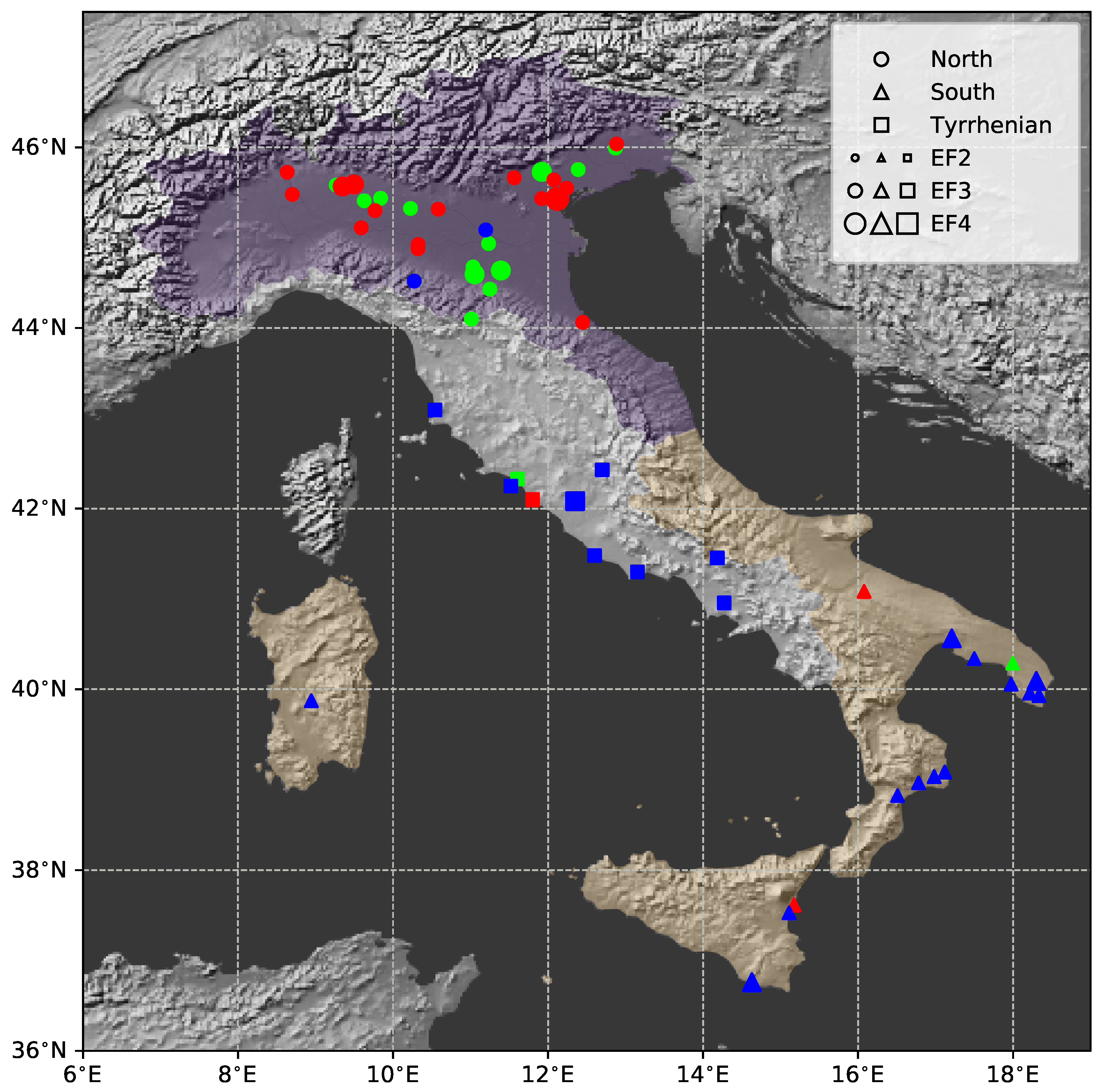
Figure 1 shows the geographical distribution, category and season of the tornadoes considered here. The dataset consists of 57 EF2+ events: 15 occurred in spring, 19 in summer, and 23 in autumn. The winter season is discarded because too few significant tornadoes are present, which makes the corresponding seasonal characterization statistically very weak.
2.2. Reanalysis Datasets
The data used in this work are extracted from two global reanalysis datasets: ERA-Interim [45] and ERA-5 [46], which, respectively, have an approximate resolution of 80 km (0.75°) and 31 km (0.25°), with 60 and 137 vertical levels from the surface up to 0.1 hPa. The data are extracted every 6 h for the u (West-East) and v (South-North) components of WS and for CAPE. Although in principle shorter time steps are possible (since hourly ERA-5 data are available), for the sake of comparison between the two datasets, a 6 h time resolution of CAPE in ERA-Interim [47] dictated such a choice. A known error in the way ERA-Interim calculated CAPE produces zero values in the 3 h forecast, and prevents to download CAPE at regular 3 h time steps https://confluence.ecmwf.int/display/CKB/ERA-Interim+known+issues).
2.3. Meteorological Parameters
As shown in Section 1, the scientific literature indicates the vertical wind shear (WS) and the convective available potential energy (CAPE) among the most relevant variables for the formation of tornadoes; for this reason, in the following, we will consider them as the variables of interest. Indeed, in mesocyclonic tornadoes, the vertical vorticity is partly generated by the tilting of the horizontal component of vorticity that is associated with vertical WS, while CAPE is a good predictor of the maximum updraft speed [23]. This represents a first step of the analysis, with the aim of extending the investigation to other variables that may be equally informative about the possible occurrence of tornadoes (e.g., storm relative helicity).
For each event, WS and CAPE are calculated at the closest grid point on the upstream side of the location where the tornado has occurred. Four Time-Steps (TS) before the event are considered for each tornado. Taking into account the 6 h resolution at which data are extracted, this allows checking the temporal evolution of the parameters of interest in the 24 h before the tornado. The Time Step closest to the tornado occurrence (i.e., from 0 to 6 hours before) is denoted as “TS1”, while “TS2”, “TS3”, and “TS4” correspond to, respectively, time ranges of 6–12, 12–18, and 18–24 h before the event. While 24 h may appear too long for fast-changing variables, such as CAPE, one should consider that we plan to extend our analysis to climate simulations; thus, it appears natural to work with the same time resolution available in such runs, and see if any signal is present within this time frame.
- Wind shear (LLS, DLS). WS is computed as the magnitude of the vector representing the difference between the wind near the surface and at a fixed level in the air column. Two parameters are considered, the low-level shear (LLS) and the deep-level shear (DLS), representing the differences between the wind speed near the surface (1000 hPa) and at about 1 km and 6 km (900 hPa and 500 hPa, respectively). Although LLS and DLS are not calculated within the generally used 0–1km and 0–6 km layers, our different choice does not affect the results, also considering that all the analyzed tornadoes occur in flat regions (only one case is recorded above 300 m). It is important to highilight that previous studies [48,49] reveal that atmospheric reanalysis tends to underestimate the low-level shear compared to sounding observations.
- Updraft Maximum Vertical Velocity (WM). CAPE [50,51,52] represents the available potential energy. It is defined as , where z is the height, is the buoyancy force, is the Level of Free Convection, is the Equilibrium Level, and and are the virtual temperature of the air parcel and of the surrounding environment, respectively [23,53].The buoyancy produces the vertical acceleration of the air parcels: , where w is the vertical velocity component and t is time. In the reanalyses used in this work, CAPE is extracted from ECMWF, calculated as the maximum value among the air parcels lifted from different model levels below 350 hPa (MUCAPE). In this study, CAPE is expressed via the Updraft Maximum Vertical Velocity (WM), supposing that the buoyancy is the only active force according to the Parcel Theory: i.e., [23,53]. WM is computed at the same grid points and times as WS01 and WS06.
- Standardized values. To obtain comparable dimensionless indices, a standardization is applied. The generic index I is defined as , where X is the value of the parameter of interest (WM, LLS, or DLS). The mean value (climatological mean), as well as the standard deviation , are computed separately for each tornado, considering the 19 values of the parameter I at the same hour and calendar day when the tornado occurred for the years 2000–2018. Therefore, and have different values for each individual tornado, both for the ERA-5 and the ERA-Interim datasets.
2.4. Statistical Tools and Procedures
Below, we briefly describe the adopted statistical tools and procedures.
2.4.1. Homogeneity Tests
The Kolmogorov—Smirnov (KS) and the Anderson–Darling (AD) are two-sample homogeneity tests commonly used to check whether two variables have the same probability distribution [54,55]. They allow rejection of the Null Hypothesis “: the probability distribution of the variables extracted from two different samples is the same”. The KS test is indicated to spot possible differences in the body of the distributions, while AD is suggested for detecting possible dissimilarities in the tails. Instead, the Mann–Whitney (MW) test [56] is used to check whether the difference in central tendency (such as the mean, the median and the mode) of two populations differs from zero. These tests are used in Section 3.1 and Section 3.2.
2.4.2. Conditional Probabilities
An attempt to estimate the probability of tornado occurrence, conditional to the fact that WM (or LLS, or DLS) takes on values in a given range just before the event (i.e., at time step TS1), is carried out.
For each parameter (WM, or LLS, or DLS) the range spanned by the variable is first partitioned into K sub-intervals ’s, with . Then, the number of times that a specific parameter takes on a value in the interval is computed, for . Finally, the number of tornadoes when the parameter has taken on a value in is calculated. In turn, the conditional probability of interest is given by
where X denotes either WM, or LLS, or DLS. The uncertainty affecting the estimates of the ’s is assessed via suitable Bootstrap (Monte Carlo) procedures [57].
Since no physical indications exist that could help choosing the values for ’s, here a reasonable statistical strategy is adopted. Specifically, the K sub-intervals are picked out in such a way that they contain approximately the same number of tornadoes. The choice represents a compromise between a significant number of bins and a sufficient number of tornadoes in each sub-interval: practically, they correspond to the first, second, third, and fourth inter-quartile range of the parameter of interest. For convenience, the bins are labelled as “Low”, “Medium”, “High”, and “Extreme”. The ’s used in this work are shown in Table 1. (A different number of events characterizes the datasets ERA-5 and ERA-INTERIM: respectively, 57 and 55. The reason is that the lower resolution in ERA-INTERIM does not allow differentiation of some events that occurred at close times in similar locations.)
2.4.3. Multivariate Analysis via Copulas
Copulas represent a convenient and efficient tool to model the joint random behavior of a set of variables (here, the trivariate vector (WM, LLS, DLS)) ruling the statistics of the phenomenon of interest (here, the occurrence of a tornado). For a theoretical introduction to copulas, see Nelsen [58], Joe [59], Durante and Sempi [60]; for a practical approach see Salvadori et al. [61].
In particular, copulas are multidimensional functions mathematically formalizing the statistical dependence among the variables of interest. According to the Sklar’s Theorem representation [62]—i.e., Equation (2) below, copulas allow construction of the joint distribution of the ’s, with marginal distributions ’s, as
for all , where is the copula associated with the random vector ; here, .
In the present case, according to the Kendall and Spearman independence tests [58,61], WM is statistically independent of both LLS and DLS, whereas LLS and DLS are dependent on each other. As a consequence, a trivariate copula model for the vector (WM, LLS, DLS) can be set up as [61]
for all (the natural domain of a trivariate copula, since its arguments are probability distribution functions ranging in ), where denotes the (marginal) bivariate copula of (LLS, DLS).
Here, can be taken as a member of the Frank family of copulas [58,61], since it adequately fits the (LLS, DLS)’s data: in fact, the Goodness-of-Fit p-Value is larger than 10%, for both the ERA-5 and the ERA-Interim reanalyses. The analytical expression of is presented in Appendix A.
3. Results
3.1. Relevance of Geographical and Seasonal Features
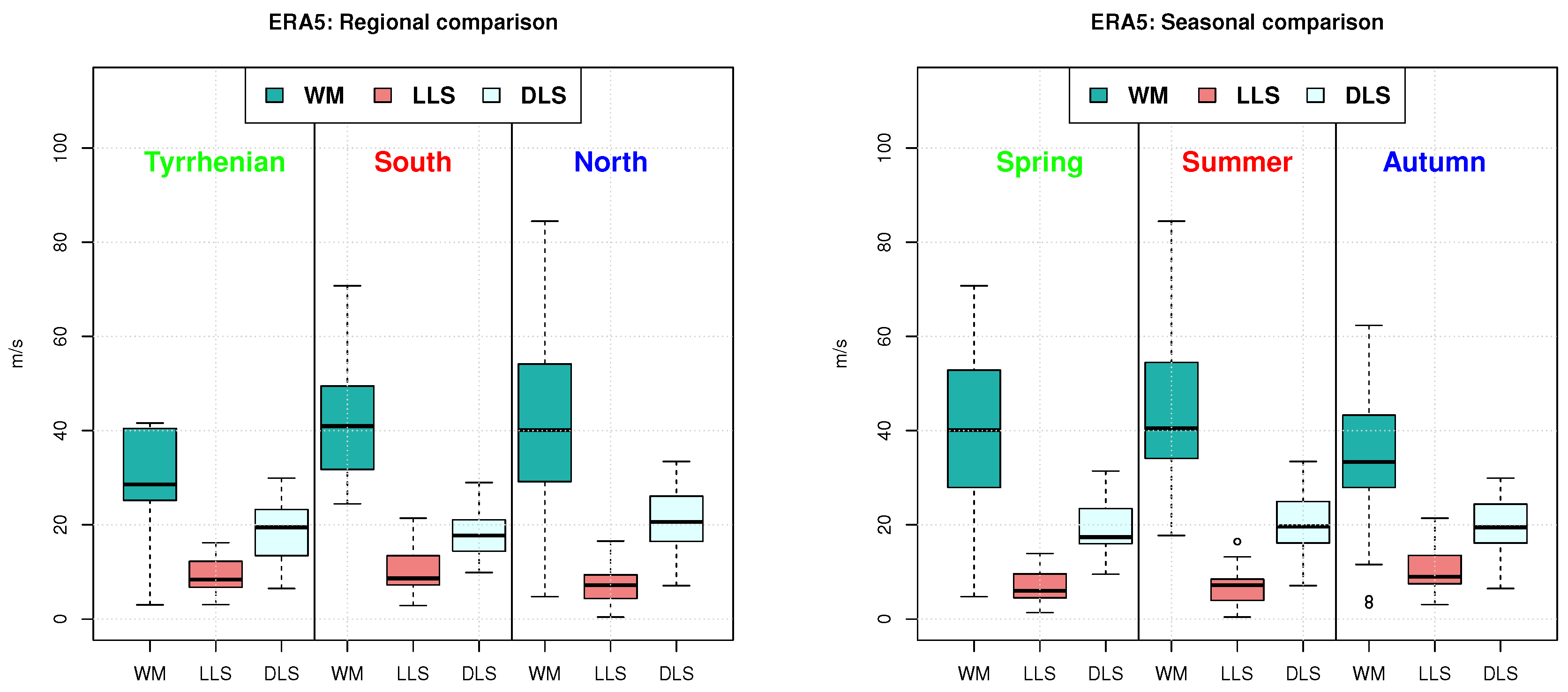
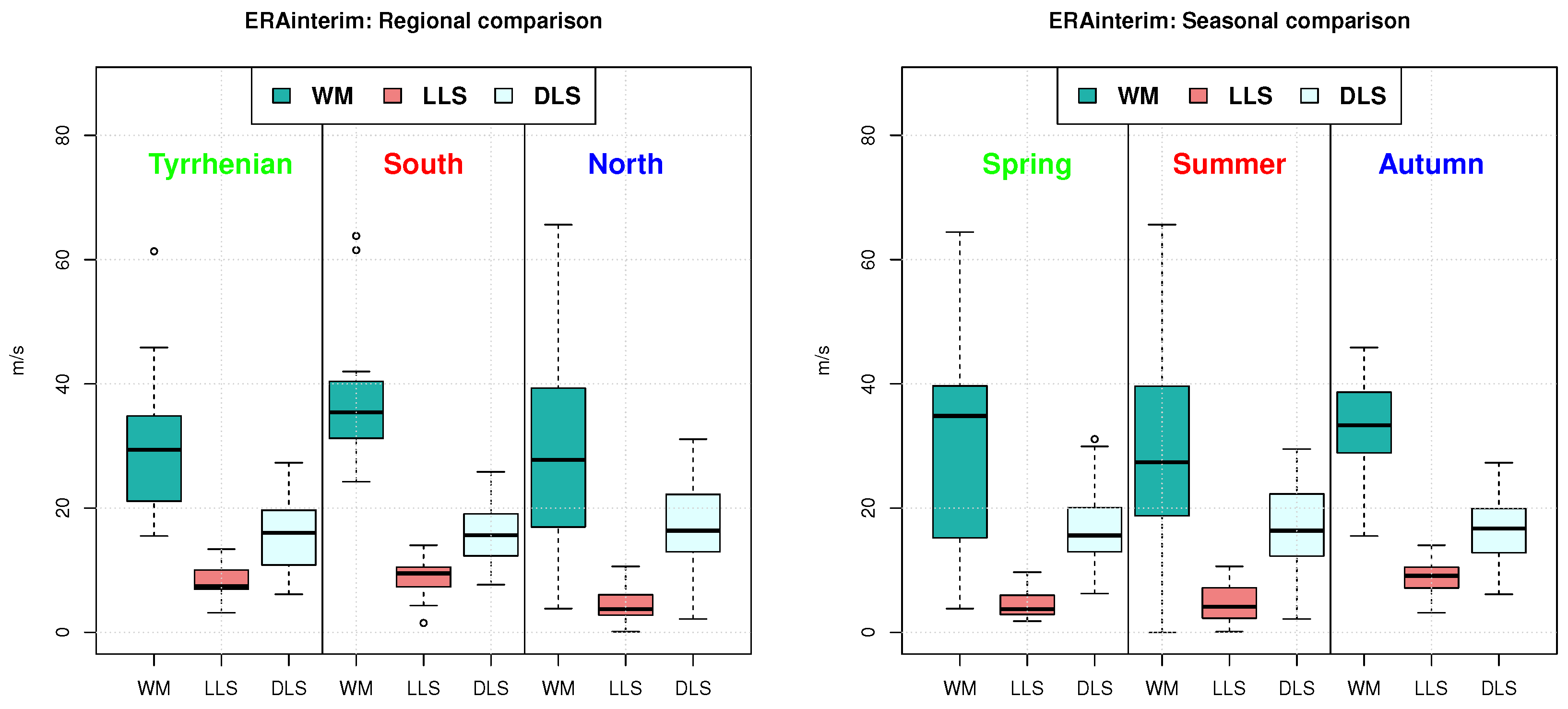
Figure 1 shows that in northern Italy, tornadoes typically occur in spring and summer, whereas those affecting the Tyrrhenian coast and southern Italy are more common in autumn. However, according to the KS test, WM (as well as LLS and DLS) shows no statistically different behavior neither among the three sub-regions (as in Figure 3-left), nor among seasons (as in Figure 3-right), for both the ERA-5 and the ERA-INTERIM dataset (the latter plotted in Figure A2). The p-values reported in Table 2 are generally larger than 5%. Note that the AD and the MW tests lead to similar conclusions.
There is one main exception: LLS takes on values generally smaller in the northern region than in southern and Tyrrhenian ones (Figure 3-left and Figure A2-left), and it takes on values in Autumn generally larger than in Spring and Summer (Figure 3-right and Figure A2-right). These results seem consistent, since Autumn cases occur mainly in Tyrrhenian and southern regions. The visual analysis is supported by the combined p-values of the three statistical tests (KS, AD, and MW) reported in Table 2. Regarding the regions, ERA-Interim shows significant differences in LLS between the north and the other regions, which is not the case for ERA-5 (p-values are high). Therefore, in the following, the data will be pulled together and investigated, irrespectively of the region and the season of tornado occurrences analyzed. This strategy will also increase the sample size, leading to more robust statistical results.
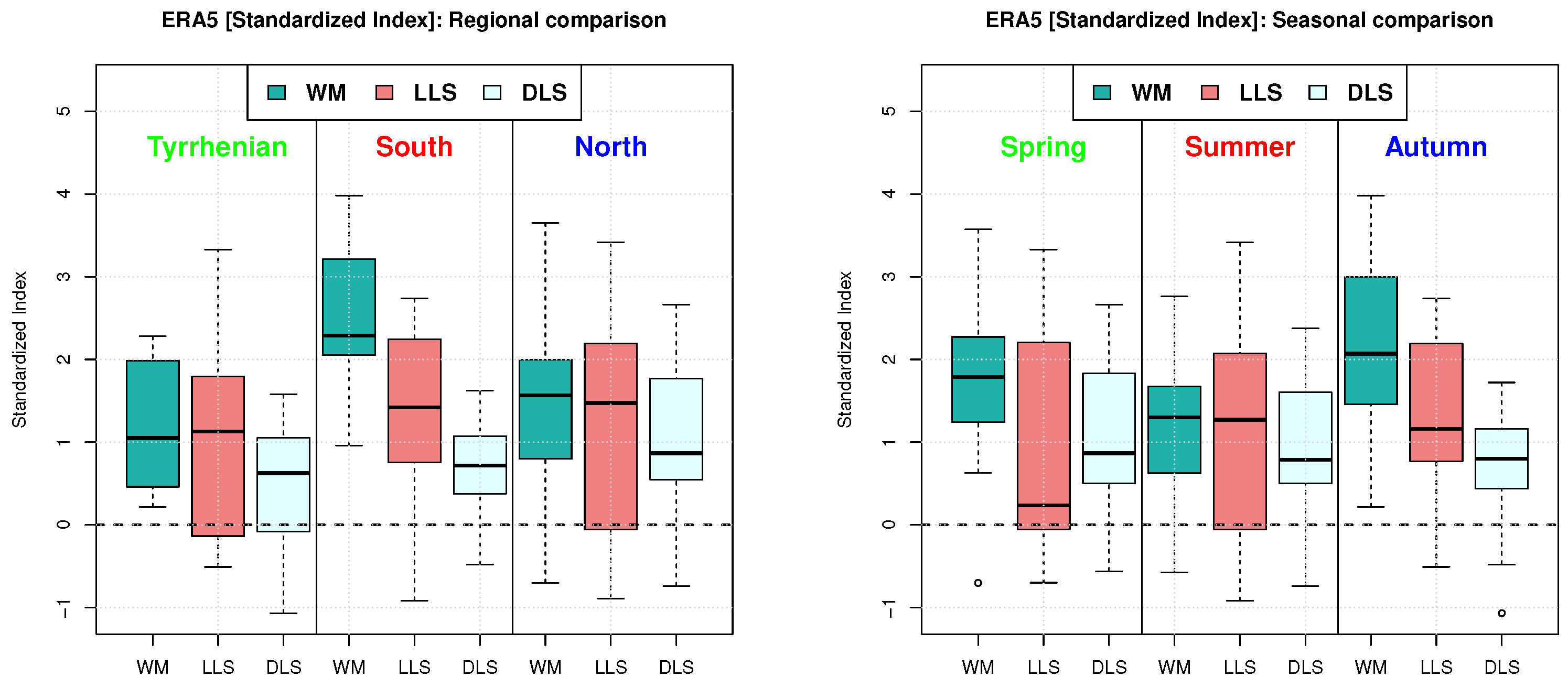
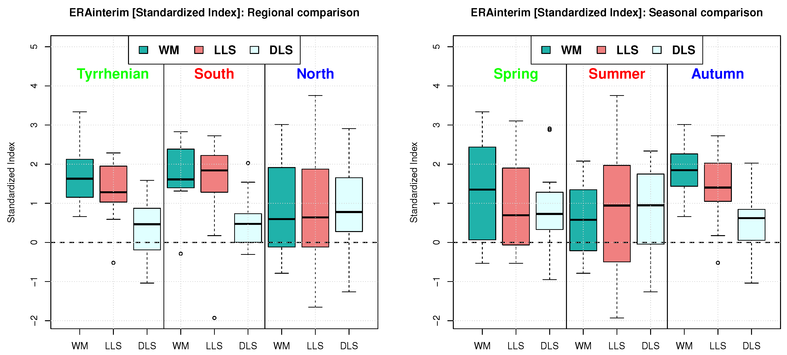
The analysis of the Standardized indices shows to what extent the values of WM, LLS, and DLS corresponding to the occurrence of tornadoes differ from regional and seasonal mean climate conditions. In other words, the standardized indices provide somewhat different information as compared to the actual values of these parameters, since they may spotlight possible differences with respect to the mean climate when a tornado occurs. Here, the main point is that values of a standardized index larger than zero indicate that the corresponding variable takes on values larger than the average climate, and thus the crucial question is simply whether or not (and to what extent) an index is significantly larger than zero.
The boxplots presented in Figure 4 and Figure A3 show that for both the ERA-5 and the ERA-Interim datasets, the parameters WM, LLS, and DLS generally take on values (much) larger than the mean climate conditions just before the occurrence of a tornado. In some cases, all the index values are strictly positive (e.g., WM in Tyrrhenian and southern regions, and in Autumn). In general, (at least) 75% of the index values are larger than zero.
3.2. Evolution of WS and CAPE before a Tornado Occurrence
The distribution of the parameters LLS, DLS, and WM as observed at time steps TS1 and TS4—i.e., respectively, in the intervals 0–6 h and 18–24 h before the occurrence of a tornado—are statistically compared in Table 3, where the p-values of the KS and AD Homogeneity tests are shown, for both ERA-Interim and ERA-5 reanalyses. The results show that all three parameters take on values that immediately before the occurrence of a tornado (i.e., at TS1) are significantly different from the ones at the earlier time step TS4. In fact, all the p-values are smaller than 5%, with the only exception the KS test for DLS in ERA-5 (but the corresponding AD test yields 1.1%).
Consequently, the distributions of WM, LLS, and DLS at TS1 and TS4 turn out to be statistically different. These results, put together with those presented in Section 3.1, support the claim that large values of WM, LLS, and DLS may be robust precursors of the genesis of a tornado, especially if their magnitude is assessed with respect to the background local climatology.
3.3. Conditional Probability of Tornado Occurrence
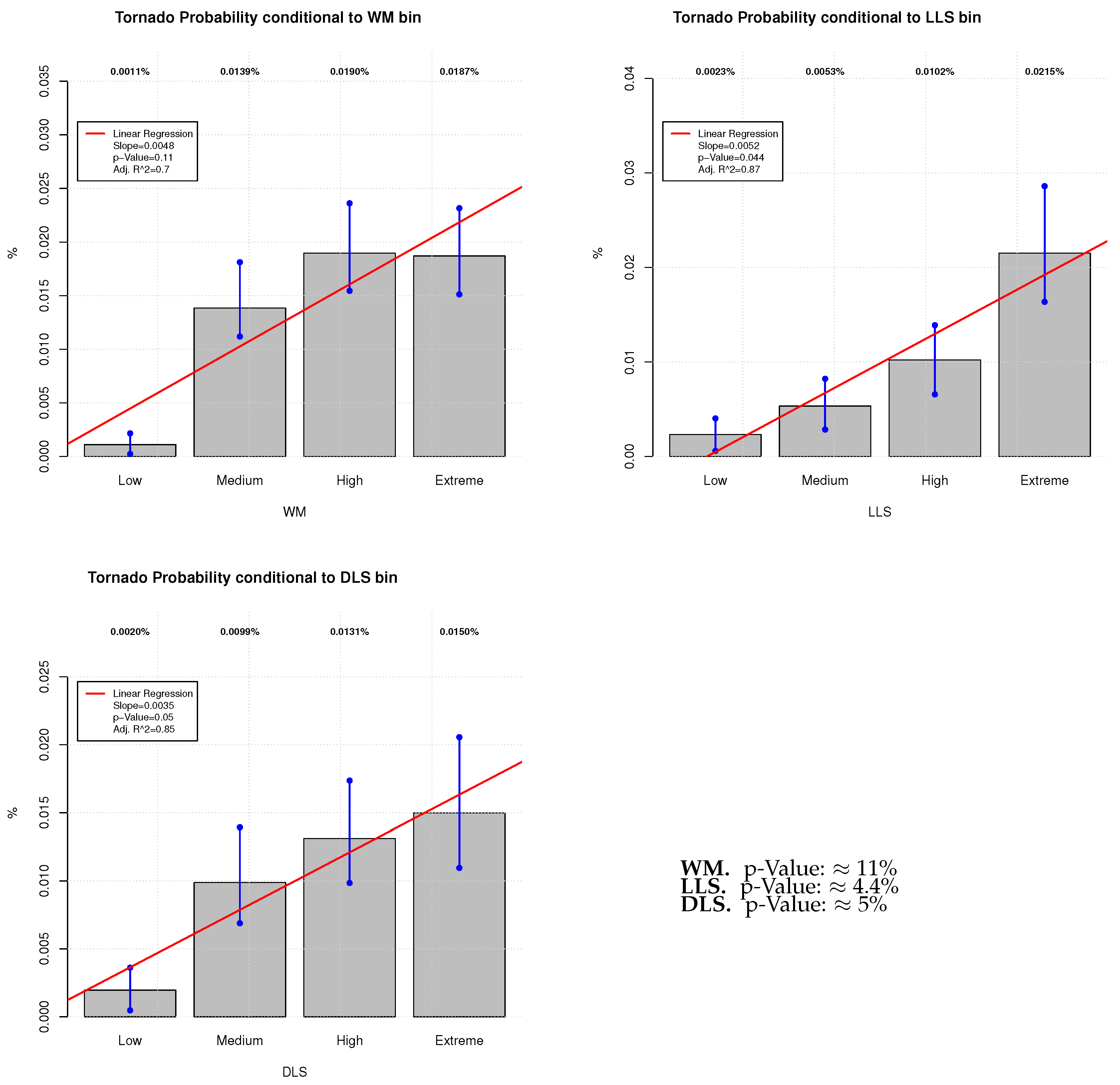
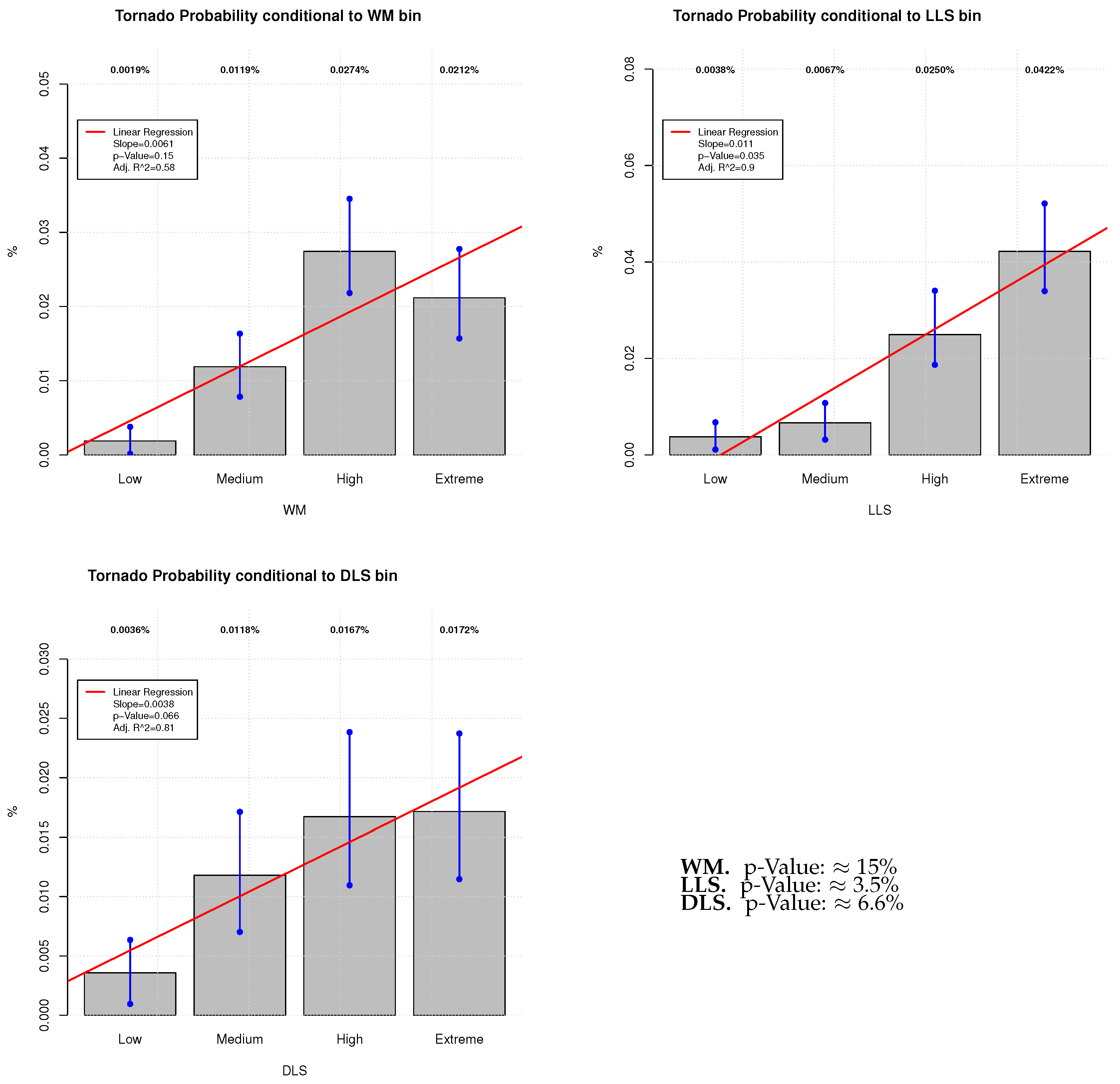
The estimate of the probability of tornado occurrence p, conditional to the fact that WM (or LLS, or DLS) takes on a value in a given sub-interval at TS1 (see Section 2.4), is plotted in Figure 5 for the ERA-5 dataset—the ERA-Interim case is illustrated in Figure A4.
A main goal of our study is to provide a statistical relation between the probability ’s and the magnitude of the considered parameters (WM, LLS, DLS). For this purpose, a linear regression is carried out, using the ’s as a response, and the sub-intervals index as a predictor. Then, the (statistical) admissibility of a non-constant linear trend is checked via the p-Value associated with the slope of the regression line. Figure 5 shows the fitted lines, as well as the corresponding p-values. As a result, at a standard 5% level, the (conditional) probability of tornado occurrence is likely to increase as LLS (or DLS) increases (regression p-values, respectively, ≈ 4.4% and ≈ 5%), whereas the statistical evidence of a similar growth for WM (p-Value ≈ 11%) might be questionable. The analysis of the ERA-Interim datasets leads to similar conclusions.
The probability is estimated only in locations where tornadoes occurred, i.e., it is valid where morphological conditions allow their formation. In idealized conditions, Markowski and Dotzek [63] showed that the orography has the effect of enhancing convective inhibition and reducing relative humidity; accordingly, there is a tendency for the supercells to weaken in mountainous areas. Hence, although the development of tornadoes may be occasionally favored by the presence of mountains [18], they preferentially develop over flat terrain.
3.4. Multivariate Analysis of Tornado Occurrence
As anticipated in Section 2.4, the construction of a trivariate probabilistic model of the joint random behavior of the vector (WM, LLS, DLS) is carried out by using Copulas. As a novelty, the (physically) expected fact that low-level WS is more correlated with deep-layer wind shear than CAPE is given, for the first time, a (statistical) analytical multivariate model. On the one hand, the copula framework proposed here is able to “qualify” the type of dependence, via the selection of a suitable admissible copula family (i.e., different copulas identify different dependence models). On the other hand, it possible to objectively “quantify” the strength of the statistical dependence: e.g., via the estimate of the copula parameter, which is in a one-to-one relation with measures of concordance such as the Kendall and Spearman rank correlation coefficients. In summary, the copula framework outlined here provides a valuable model of the (analytical/statistical) relationships between the variables at play, and furnishes easy formulas for, e.g., setting up models of their joint behavior, including conditional relations (see Equation (3.26) in Salvadori et al. [61]).
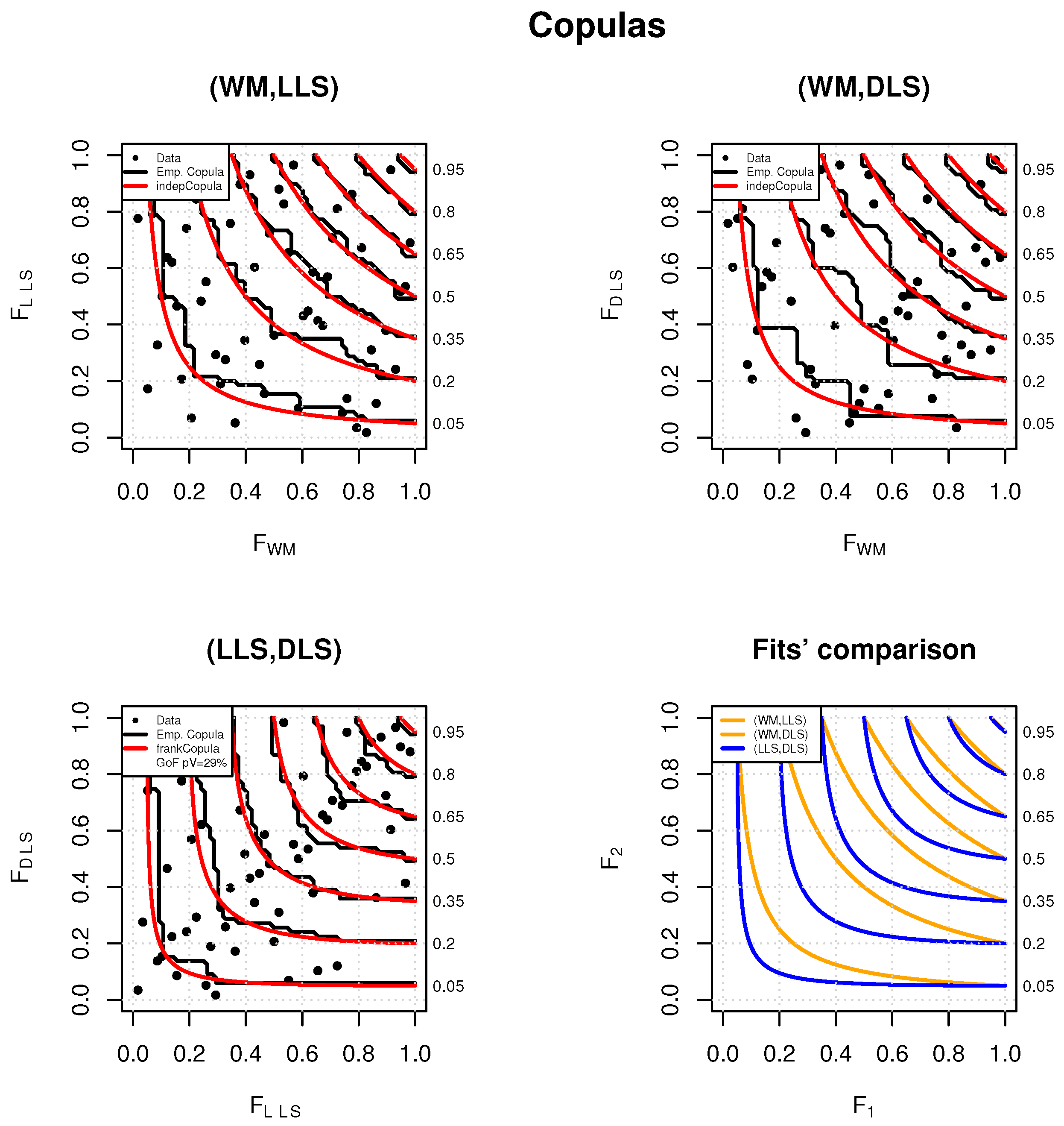
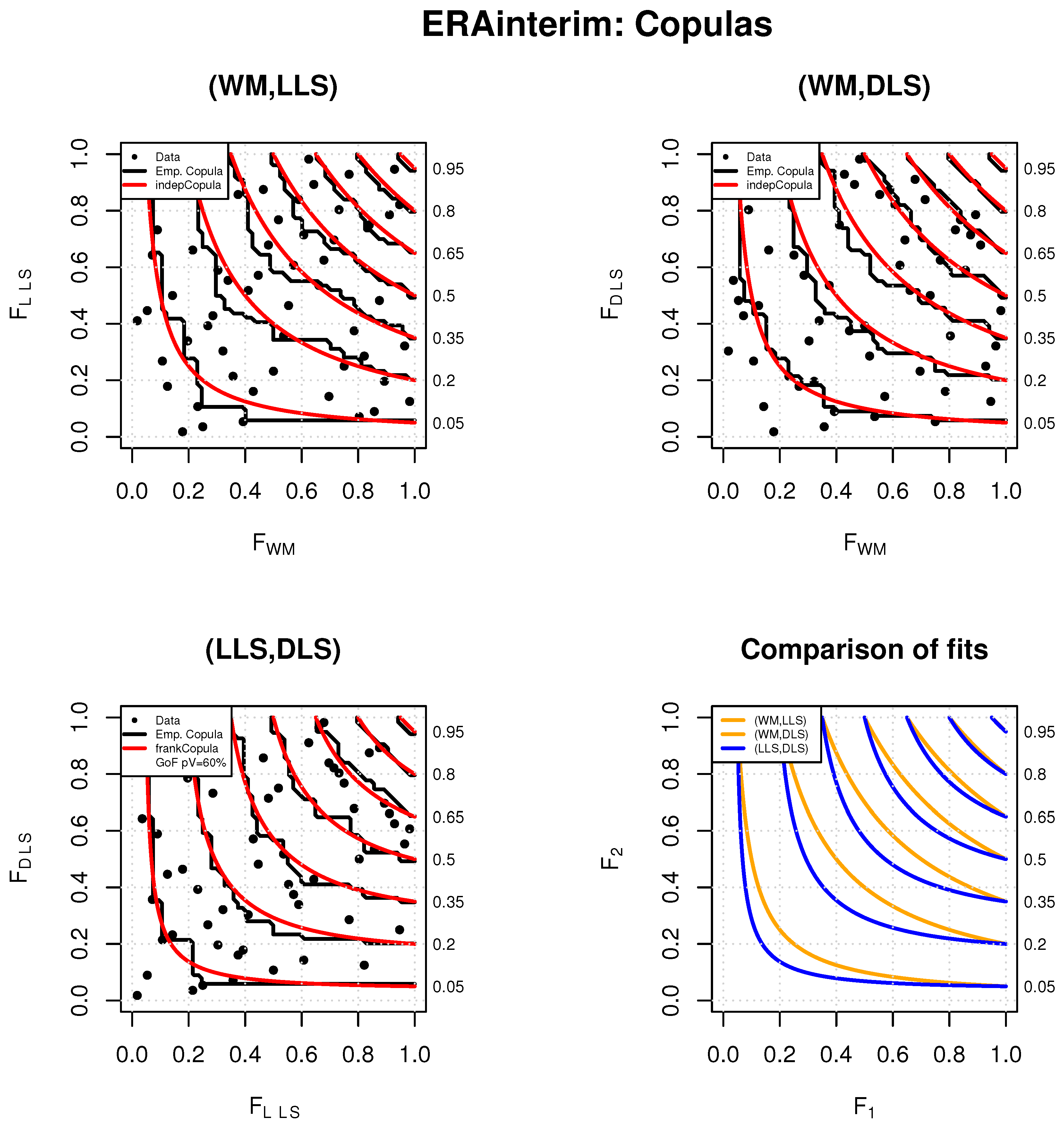
Figure 6 shows the bivariate copulas fitted on the pairs (WM, LLS), (WM, DLS), and (LLS, DLS) for the ERA5 dataset—the ERA-Interim case is presented in Figure A5. Obviously, the full trivariate copula cannot be plotted, since its visualization would require a 4-dimensional space. Also shown are the corresponding empirical copulas, i.e., the non-parametric approximations of the true (but unknown) copulas actually ruling the joint random behavior of the pairs of interest. A comparison of the three bivariate fitted copulas is shown in the bottom-right panel (note that the two copulas fitted on the pairs (WM, LLS) and (WM, DLS) are identical, and overlap).
Overall, it is clear that there is no association between WM and LLS, as well as between WM and DLS: actually, the observations are uniformly arranged in the unit square, entailing that the corresponding copula is the one modeling independent variables—this is also supported by the large p-values of the Kendall and Spearman independence tests [61]. Instead, LLS and DLS turn out to be fairly concordant (i.e., positively correlated): small/large values of LLS are likely to be associated with small/large values of DLS (and vice-versa). The bottom-right panel of Figure 6 shows the remarkable differences between the Independence copula modeling the pairs (WM, LLS) and (WM, DLS), and the Frank copula modeling (LLS, DLS).
Figure 6 suggests that the probability of occurrence of tornadoes is independently controlled by CAPE (represented by WM) and WS (represented either by LLS or DLS). In addition, the roles played by LLS and DLS are to some extent “exchangeable”, since the corresponding copula is symmetric. In other words, there is no indication that the role of the WS as a precursor of tornadoes is better described by LLS than by DLS. This suggests that when tornadoes are formed, generally, a strong horizontal shear is present in the lower half of the troposphere, as well as in the lowest layers. The analysis of the ERA-Interim case leads to similar conclusions.
4. Conclusions
In this study, we have estimated the probability of occurrence of significant (EF2+) tornadoes as a function of three parameters: LLS, DLS, and WM. What we call here LLS and DLS are the difference between the wind vector near the surface and at the 1 and 6 km level, respectively, and are representative of the WS in the lower and middle troposphere. WM, the updraft maximum vertical velocity, is derived from CAPE. The values of these three parameters have been extracted from the ERA-5 and ERA-Interim reanalyses. The information on location and intensity of tornadoes has been provided by a dataset containing Tornadoes that occurred in Italy in the period 2000–2018.
Regional and seasonal differences of these three parameters at the time closest to the tornado occurrence appears not to be significant, and allow us to analyze all events independently of the geographical location and season.
All three parameters (WM, LLS and DLS) are important precursors of significant tornadoes. In fact, at the time closest to the tornado occurrence, their values are significantly different from those observed one day before and from the climatological means.
The values of WM, LLS, DLS have been partitioned into four bins, qualitatively representing “Low”, “Medium”, “High”, and “Extreme” values. In particular, the (conditional) probability of occurrence of tornadoes is significantly different from zero when the parameters take on “Medium” (or larger) values, and especially when WM, LLS and DLS take on values in the “Extreme” bin. Similar results are obtained with a different methodology by Taszarek et al. [36], where the highest probability of tornado occurrence corresponds to environments with high deep-layer shear and moderate CAPE. Brooks [24] found that the probability of tornado-spawning thunderstorms increases with increasing values of DLS, in agreement with our results. Furthermore, the (conditional) probability of occurrence significantly increases with the magnitude of LLS and DLS, showing that the probability increases for larger WS. The same evidence is uncertain for WM. In this case, the analysis suggests that the probability of tornado occurrence becomes significant only for “Medium” to “Extreme” values of WM, without showing an increasing trend. This result suggests that tornadoes require WM to be larger than a minimum threshold, but their probability does not increase with increasing WM.
The joint probability distribution of the parameters (WM, LLS, DLS) suggests that LLS and DLS are dependent on one other, but independent of WM. Since LLS and DLS are (statistically) exchangeable, either of the two parameters can be used a predictor of tornadoes. In addition, given the results of the multivariate analysis, the role of CAPE “alone” regarding the generation of tornadoes is somewhat peculiar, and may deserve further investigation.
This study has implicitly allowed a comparison between the new ERA-5 and the former ERA-Interim datasets, suggesting that the latter underestimates the actual values of the considered precursors [49]. Although, in general, ERA-5 tends to produce larger values of all parameters than ERA-Interim before the formation of tornadoes, the results of the statistical analysis are substantially equivalent for both databases in terms of relevance and timing of the characteristics of the considered precursors. This suggests that our results are robust and do not depend on the reanalysis dataset that is used. Many climate change simulations cannot afford the space resolution of ERA5 and are comparable to ERA-Interim. The validity of our conclusions for both datasets is a useful support for their future use in climate change simulations.
There are open issues deserving further investigation, such as refining the assessment of the dependence of tornado probability on CAPE, eventually identifying its minimum value for their occurrence. Furthermore, the validation of this probability model with a larger tornado dataset, representative of other regions in the world, and a higher temporal resolution, as allowed by ERA-5 reanalysis, will be important.
The study has produced a quantitative estimate of the increasing probability of significant tornadoes with increasing WS. It has, moreover, confirmed the relevance of CAPE and assessed quantitatively the probability of tornadoes when CAPE takes on “Medium” to “Extreme” values. Finally, it has shown the relevance of the combined values of WS and CAPE on the probability of tornadoes, showing that large values can independently support their formation.
Author Contributions
Conceptualization, R.I., P.L. and M.M.M.; methodology, P.L. and M.M.M.; software, R.I. and G.S.; formal analysis, R.I. and G.S. All authors have read and agreed to the published version of the manuscript.
Funding
This research received no external funding.
Acknowledgments
The authors would like to thank Tommaso Grassi for the technical support.
Conflicts of Interest
The authors declare no conflict of interest.
Abbreviations
The following abbreviations are used in this manuscript:
| LLS | wind shear as the difference between the wind speed near the surface (1000 hPa) and at about 1 km (900 hPa) |
| DLS | wind shear as the difference between the wind speed near the surface and at about 6 km (500 hPa) |
| CAPE | convective available potential energy |
| WM | Updraft Maximum Vertical Velocity |
Appendix A. The Frank Family of Copulas
One of the possible analytical expressions of the Frank family of (bivariate) Copulas [58,61], used in this work to model the joint random behavior of the pair (LLS, DLS), is
where , and is a dependence parameter. In particular, the variables are negatively correlated when , and positively correlated when ; the limit case corresponds to independent variables.
Appendix B. ERA-Interim Figures
Figure A1.
Same as Figure 2 but considering the ERA-Interim dataset.
Figure A1.
Same as Figure 2 but considering the ERA-Interim dataset.

Figure A2.
Same as Figure 3 but considering the ERA-Interim dataset.
Figure A2.
Same as Figure 3 but considering the ERA-Interim dataset.

Figure A3.
Same as Figure 4 but considering the ERA-Interim dataset.
Figure A3.
Same as Figure 4 but considering the ERA-Interim dataset.

Figure A4.
Same as Figure 5 but considering the ERA-Interim dataset.
Figure A4.
Same as Figure 5 but considering the ERA-Interim dataset.

Figure A5.
Same as Figure 6 but considering the ERA-Interim dataset.
Figure A5.
Same as Figure 6 but considering the ERA-Interim dataset.

References
- Simmons, K.M.; Sutter, D.; Pielke, R. Normalized tornado damage in the United States: 1950–2011. Environ. Hazards 2013, 12, 132–147. [Google Scholar] [CrossRef] [Green Version]
- Antonescu, B.; Schultz, D.M.; Holzer, A.; Groenemeijer, P. Tornadoes in Europe: An Underestimated Threat. Bull. Am. Meteorol. Soc. 2017, 98, 713–728. [Google Scholar] [CrossRef]
- Brooks, H.E.; Lee, J.W.; Craven, J.P. The spatial distribution of severe thunderstorm and tornado environments from global reanalysis data. Atmos. Res. 2003, 67–68, 73–94. [Google Scholar] [CrossRef]
- Groenemeijer, P.; Kühne, T. A climatology of tornadoes in Europe: Results from the European severe weather database. Mon. Weather Rev. 2014, 142, 4775–4790. [Google Scholar] [CrossRef]
- Tippett, M.K.; Allen, J.T.; Gensini, V.A.; Brooks, H.E. Climate and Hazardous Convective Weather. Curr. Clim. Chang. Rep. 2015, 1, 60–73. [Google Scholar] [CrossRef] [Green Version]
- Palmieri, S.; Pulcini, A. Trombe d’aria sull’Italia. Riv. Meteorol. Aeronaut. 1978, 4, 263–277. [Google Scholar]
- Giaiotti, D.B.; Giovannoni, M.; Pucillo, A.; Stel, F. The climatology of tornadoes and waterspouts in Italy. Atmos. Res. 2007, 83, 534–541. [Google Scholar] [CrossRef]
- Miglietta, M.M.; Matsangouras, I.T. An updated climatology of tornadoes and waterspout in Italy. Int. J. Climatol. 2018, 38, 3667–3683. [Google Scholar] [CrossRef] [Green Version]
- Miglietta, M.M.; Arai, K.; Kusunoki, K.; Inoue, H.; Adachi, T.; Niino, H. Observational analysis of two waterspouts in northwestern Italy using an OPERA Doppler radar. Atmos. Res. 2020, 234, 104692. [Google Scholar] [CrossRef]
- Fujita, T.T. Proposed characterization of tornadoes and hurricanes by area and intensity. Satell. Mesometeorol. Res. Proj. 1971, 91, 42. [Google Scholar]
- Mahieu, P.; Wesolek, E. Tornado Rating in Europe with the Enhanced Fujita Scake (EF-Scale): Definition of Specific Damage Indicators for Accurate Tornado Ratings in Europe; Technical Report; KERAUNOS—Tornadoes and Severe Storms French Observatory: Nicosia, Cyprus, 2016. [Google Scholar] [CrossRef]
- Feuerstein, B.; Groenemeijer, P.; Dirksen, E.; Hubrig, M.; Holzer, A.M.; Dotzek, N. Towards an improved wind speed scale and damage description adapted for Central Europe. Atmos. Res. 2011, 100, 547–564. [Google Scholar] [CrossRef]
- Groenemeijer, P.; Holzer, A.M.; Hubrig, M.; Kühne, T.; Bock, L.; Soriano, J.d.D.; Gutiérrez-Rubio, D.; Kaltenberger, R.; van der Ploeg, B.; Strommer, G. The International Fujita (IF) Scale Tornado and Wind Damage Assessment Guide; Technical Report; ESSL: Munich, Germany, 2018. [Google Scholar]
- Meaden, J. Tornadoes in Britain: Their intensities and distribution in space and time. J. Meteorol. 1976, 1, 242–251. [Google Scholar]
- Brooks, H.; Doswell, C.A. Some aspects of the international climatology of tornadoes by damage classification. Atmos. Res. 2001, 56, 191–201. [Google Scholar] [CrossRef] [Green Version]
- Potter, S. Fine-Tuning Fujita: After 35 years, a new scale for rating tornadoes takes effect. Weatherwise 2007, 60, 64–71. [Google Scholar] [CrossRef]
- Miglietta, M.M.; Rotunno, R. An EF3 multivortex tornado over the Ionian region: Is it time for a dedicated warning system over Italy. Bull. Am. Meteorol. Soc. 2016, 97, 337–344. [Google Scholar] [CrossRef]
- Miglietta, M.; Mazon, J.; Rotunno, R. Numerical simulations of a tornadic supercell over the mediterranean. Weather Forecast. 2017, 32, 1209–1226. [Google Scholar] [CrossRef]
- Miglietta, M.; Mazon, J.; Motola, V.; Pasini, A. Effect of a positive sea surface temperature anomaly on a Mediterranean tornadic supercell. Sci. Rep. 2017, 7. [Google Scholar] [CrossRef] [Green Version]
- ARPAV. Temporali intensi di mercoledi 8 luglio in Veneto. In Relazione tornado sul Veneto; The Regional Environmental Protection Agency: Rome, Italy, 2015. [Google Scholar]
- Zanini, M.A.; Hofer, L.; Faleschini, F.; Pellegrino, C. Building damage assessment after the Riviera del Brenta tornado, northeast Italy. Nat. Hazards 2017, 86, 1247–1273. [Google Scholar] [CrossRef]
- Report2016. Il tornado di Pianiga, Dolo e Mira dell’8 luglio 2015. Available online: https://documenti.serenissimameteo.it/documents/tornado_8luglio2015_capitoli.pdf (accessed on 10 January 2020).
- Markowski, P.M.; Richardson, Y. Mesoscale Meteorology in Midlatitude; Wiley-Blackwell: Hoboken, NJ, USA, 2010. [Google Scholar]
- Brooks, H.E. Severe thunderstorms and climate change. Atmosp. Res. 2013, 123, 129–138. [Google Scholar] [CrossRef]
- Rotunno, R.; Klemp, J. On the Rotation and Propagation of Simulated Supercell Thunderstorms. J. Atmos. Sci. 1985, 42, 271–292. [Google Scholar] [CrossRef]
- Klemp, J. Dynamics Of Tornadic Thunderstorms. Ann. Rev. Fluid Mech. 1987, 19, 369–402. [Google Scholar] [CrossRef]
- Barnes, S.L. Some aspects of a severe, right-moving thunderstorm deduced from mesonet rawinsonde observations. Geophys. Fluid Dyn. 1970, 4, 147–158. [Google Scholar] [CrossRef]
- Schlesinger, R.E. A Three-Dimensional Numerical Model of an Isolated Deep Convective Cloud: Preliminary Results. J. Atmos. Sci. 1975, 32, 934–964. [Google Scholar] [CrossRef] [Green Version]
- Rotunno, R. On the Evolution of Thunderstorm Rotation. Mon. Weather Rev. 1981, 109, 577–586. [Google Scholar] [CrossRef] [Green Version]
- Markowski, P.M.; Richardson, Y.P. Tornadogenesis: Our current understanding, forecasting considerations, and questions to guide future research. Atmos. Res. 2009, 93, 3–10. [Google Scholar] [CrossRef]
- Weisman, M.L.; Rotunno, R. The Use of Vertical Wind Shear versus Helicity in Interpreting Supercell Dynamics. J. Atmos. Sci. 2000, 57, 1452–1472. [Google Scholar] [CrossRef] [Green Version]
- Markowski, P.M.; Richardson, Y.P. The Influence of Environmental Low-Level Shear and Cold Pools on Tornadogenesis: Insights from Idealized Simulations. J. Atmos. Sci. 2014, 71, 243–275. [Google Scholar] [CrossRef]
- Colquhoun, J.R.; Shepherd, D.J. An Objective Basis for Forecasting Tornado Intensity. Weather Forecast. 1989, 5, 35–50. [Google Scholar] [CrossRef] [Green Version]
- Thompson, R.L.; Edwards, R.; Hart, J.A. Close Proximity Soundings within Supercell Environments Obtained from the Rapid Update Cycle. Weather Forecast. 2003, 18, 1243–1261. [Google Scholar] [CrossRef] [Green Version]
- Dupilka, M.L.; Reuter, G.W. Forecasting Tornadic Thunderstorm Potential in Alberta Using Environmental Sounding Data. Part I: Wind Shear and Buoyancy. Weather Forecast. 2006, 21, 325–335. [Google Scholar] [CrossRef]
- Taszarek, M.; Brooks, H.E.; Czernecki, B. Sounding-Derived Parameters Associated with Convective Hazards in Europe. Mon. Weather Rev. 2017, 145, 1511–1528. [Google Scholar] [CrossRef]
- Grünwald, S.; Brooks, H. Relationship between sounding derived parameters and the strength of tornadoes in Europe and the USA from reanalysis data. Atmos. Res. 2011, 100, 479–488. [Google Scholar] [CrossRef]
- Púčik, T.; Groenemeijer, P.; Rýva, D.; Kolář, M. Proximity Soundings of Severe and Nonsevere Thunderstorms in Central Europe. Mon. Weather Rev. 2015, 143, 4805–4821. [Google Scholar] [CrossRef]
- Rodriguez, O.; Bech, J. Sounding-derived parameters associated with tornadic storms in Catalonia. Int. J. Clim. 2017, 38, 2400–2414. [Google Scholar] [CrossRef] [Green Version]
- Groenemeijer, P.; van Delden, A. Sounding-derived parameters associated with large hail and tornadoes in the Netherlands. Atmos. Res. 2007, 83, 473–487. [Google Scholar] [CrossRef]
- Thompson, R.L.; Smith, B.T.; Grams, J.S.; Dean, A.R.; Broyles, C. Convective Modes for Significant Severe Thunderstorms in the Contiguous United States. Part II: Supercell and QLCS Tornado Environments. Weather Forecast. 2012, 27, 1136–1154. [Google Scholar] [CrossRef] [Green Version]
- Craven, J.; Brooks, H. Baseline climatology of sounding derived parameters associated with deep, moist convection. Natl. Weather Dig. 2004, 28, 13–24. [Google Scholar]
- Rasmussen, E.N.; Blanchard, D.O. A Baseline Climatology of Sounding-Derived Supercell and Tornado Forecast Parameters. Weather Forecast. 1998, 13, 1148–1164. [Google Scholar] [CrossRef] [Green Version]
- Grams, J.S.; Thompson, R.L.; Snively, D.V.; Prentice, J.; Hodges, G.M.; Reames, L.J. A Climatology and Comparison of Parameters for Significant Tornado Events in the United States. Weather Forecast. 2012, 27, 106–123. [Google Scholar] [CrossRef]
- Dee, D.; Uppala, S.M.; Simmons, A.J.; Berrisford, P.; Poli, P.; Kobayashi, S.; Andrae, U.; Balmaseda, M.A.; Balsamo, G.; Bauer, P.; et al. The ERA-Interim reanalysis: Configuration and performance of the data assimilation system. Q. J. R. Meteorol. Soc. 2011, 137, 553–597. [Google Scholar] [CrossRef]
- ECMWF. Available online: https://confluence.ecmwf.int/display/CKB/ERA5%3A+data+documentation (accessed on 10 January 2020).
- ECMWF. Available online: https://confluence.ecmwf.int/display/CKB/ERA-Interim+known+issues (accessed on 10 January 2020).
- Gensini, V.A.; Mote, T.L.; Brooks, H.E. Severe-Thunderstorm Reanalysis Environments and Collocated Radiosonde Observations. J. Appl. Meteorol. Climatol. 2014, 53, 742–751. [Google Scholar] [CrossRef]
- Taszarek, M.; Brooks, H.E.; Czernecki, B.; Szuster, P.; Fortuniak, K. Climatological Aspects of Convective Parameters over Europe: A Comparison of ERA-Interim and Sounding Data. J. Clim. 2018, 31, 4281–4308. [Google Scholar] [CrossRef]
- Moncrieff, M.W.; Miller, M.J. The dynamics and simulation of tropical cumulonimbus and squall lines. Q. J. R. Meteorol. Soc. 1976, 102, 373–394. [Google Scholar] [CrossRef]
- Doswell, C.A.; Rasmussen, E.N. The Effect of Neglecting the Virtual Temperature Correction on CAPE Calculations. Weather Forecast. 1994, 9, 625–629. [Google Scholar] [CrossRef] [Green Version]
- Emanuel, K.A. Atmospheric Convection; Oxford University Press: Oxford, UK, 1994. [Google Scholar]
- Holton, J.R. An Introduction to Dynamic Meteorology; Elsevier Academic Press: Amsterdam, The Netherlands, 2004. [Google Scholar]
- Conover, W.J. Practical Nonparametric Statistics; John Wiley & Sons: New York, NY, USA, 1971. [Google Scholar]
- Neuhaeuser, M. Nonparametric Statistical Tests, A Computational Approach; CRC Press: Boca Raton, FL, USA, 2012. [Google Scholar]
- Corder, G.; Foreman, D. Nonparametric Statistics: A Step-by-Step Approach; Wiley: Hoboken, NJ, USA, 2014; ISBN 978-1118840313. [Google Scholar]
- Davison, A.C.; Hinkley, D.V. Bootstrap Methods and Their Application; Cambridge Series on Statistical and Probabilistic Mathematics; Cambridge University Press: Cambridge, UK, 1997. [Google Scholar]
- Nelsen, R. An Introduction to Copulas, 2nd ed.; Springer: New York, NY, USA, 2006. [Google Scholar]
- Joe, H. Dependence Modeling with Copulas; CRC Monographs on Statistics & Applied Probability; Chapman & Hall: London, UK, 2014. [Google Scholar]
- Durante, F.; Sempi, C. Principles of Copula Theory; CRC/Chapman & Hall: Boca Raton, FL, USA, 2015. [Google Scholar]
- Salvadori, G.; De Michele, C.; Kottegoda, N.; Rosso, R. Extremes in Nature. An Approach Using Copulas; Water Science and Technology Library Series; Springer: Dordrecht, The Netherlands, 2007; Volume 56, ISBN 978-1-4020-4415-1. [Google Scholar]
- Sklar, A. Fonctions de répartition à n dimensions et leurs marges. Publ. Inst. Stat. Univ. Paris 1959, 8, 229–231. [Google Scholar]
- Markowski, P.M.; Dotzek, N. A numerical study of the effects of orography on supercells. Atmos. Res. 2011, 100, 457–478. [Google Scholar] [CrossRef] [Green Version]
Figure 1.
Locations of EF2+ tornadoes occurred in Italy during the period 2000–2018. The colors indicate the seasons: spring (green), summer (red), and autumn (blue). Different markers represent three different regions: northern Italy (circles), the Tyrrhenian coast (squares), southern Italy (triangles). The increasing size of the markers denote stronger intensity of tornadoes (from EF2 to EF4)—see the corresponding legend.

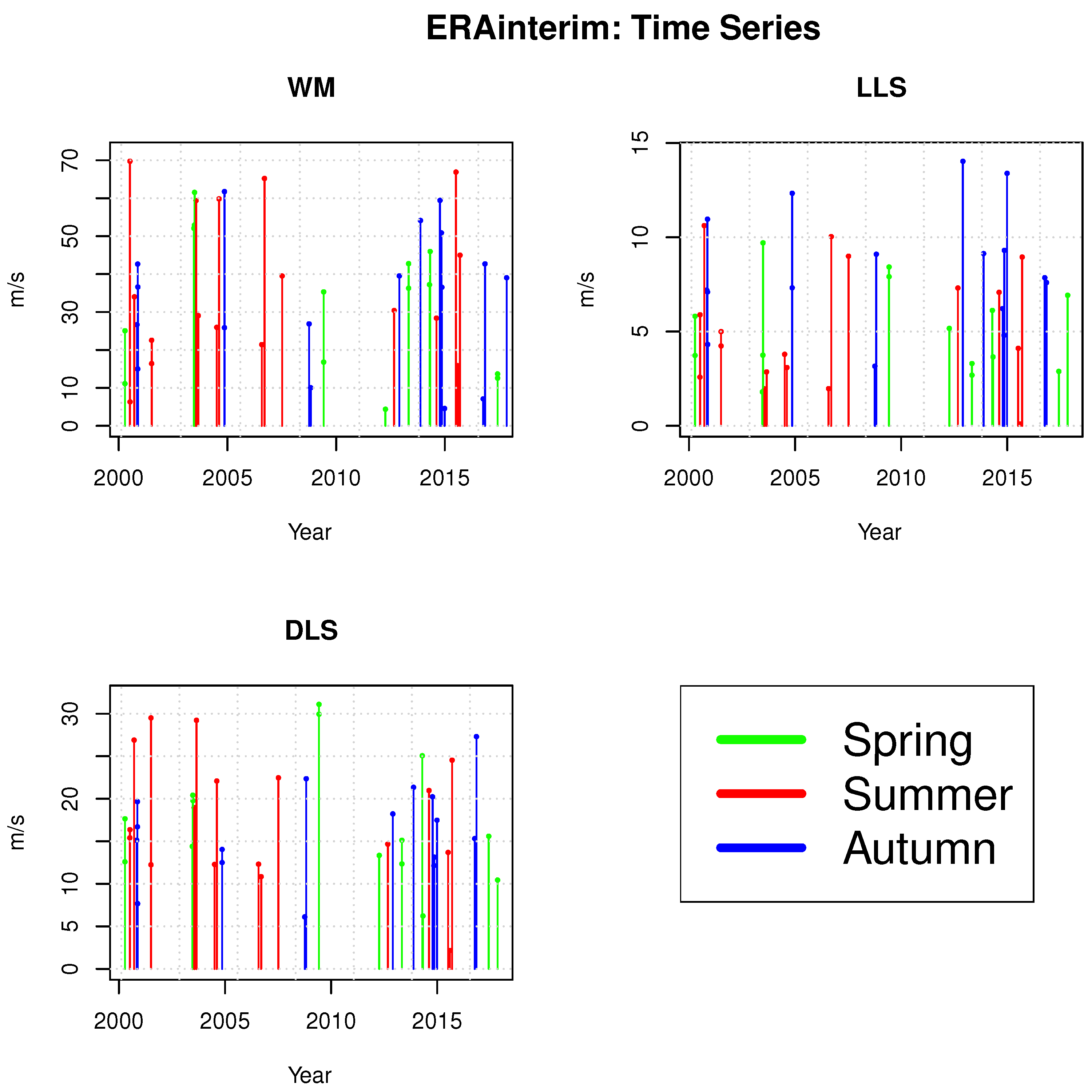
Figure 2.
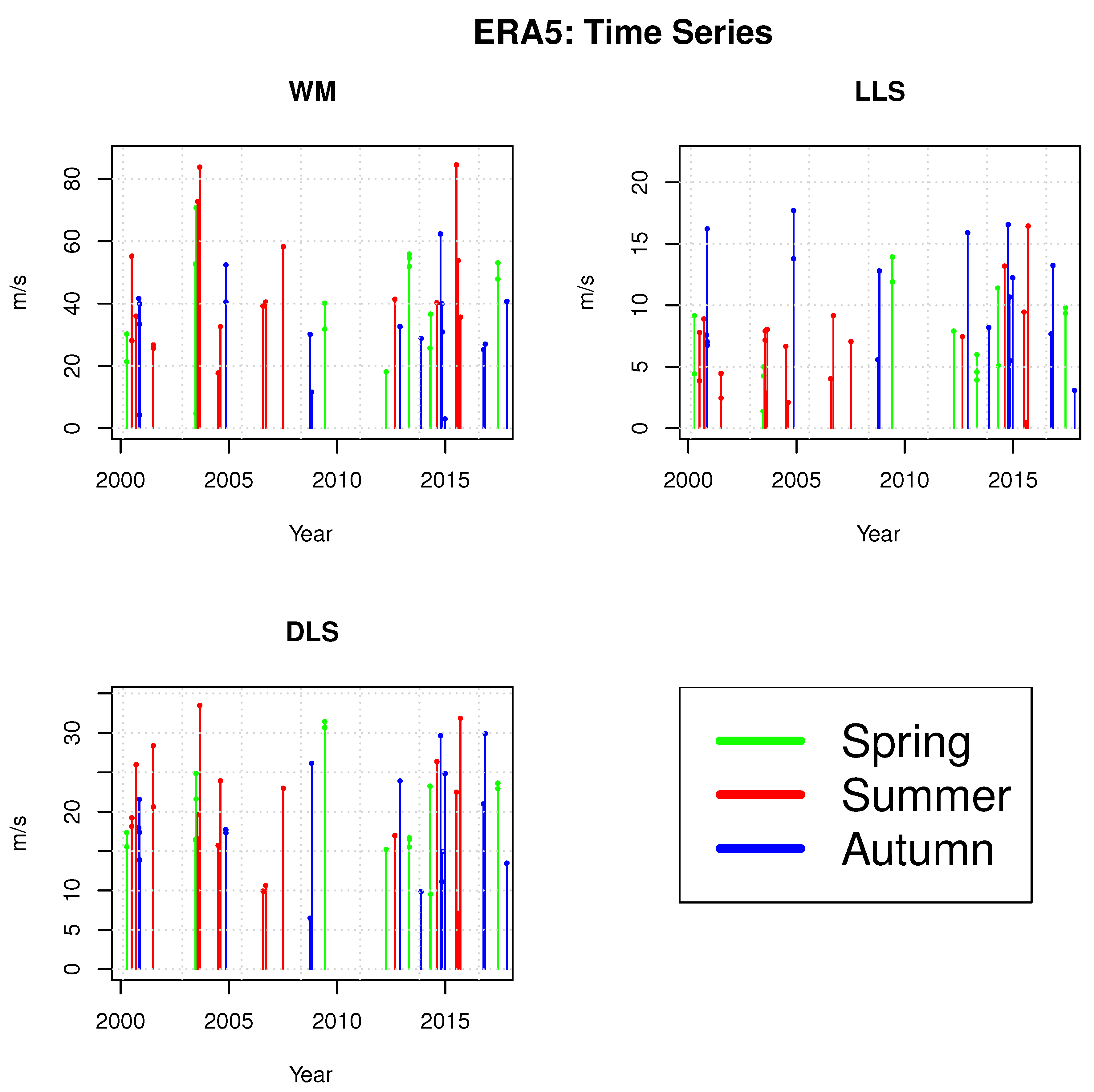
Time Series of updraft maximum vertical velocity (WM) and wind shear (LLS and DLS) extracted from ERA-5 at the 6 h time step closest to the occurrence of the tornadoes (TS1). The height of the bars indicates the magnitude of the variable, while the color marks the season when tornadoes occurred (see also Figure 1).
Figure 2.
Time Series of updraft maximum vertical velocity (WM) and wind shear (LLS and DLS) extracted from ERA-5 at the 6 h time step closest to the occurrence of the tornadoes (TS1). The height of the bars indicates the magnitude of the variable, while the color marks the season when tornadoes occurred (see also Figure 1).

Figure 3.
Boxplots of WM, LLS and DLS values in different sub-regions (left) and seasons (right) considering the ERA-5 dataset. The edges of the box indicate the 25th and 75th percentiles. The whiskers correspond to approximately 99% confidence interval.
Figure 3.
Boxplots of WM, LLS and DLS values in different sub-regions (left) and seasons (right) considering the ERA-5 dataset. The edges of the box indicate the 25th and 75th percentiles. The whiskers correspond to approximately 99% confidence interval.

Figure 4.
Same as Figure 3 but referred to Standardized indices. The horizontal black dashed line at zero corresponds to the mean climate condition.
Figure 4.
Same as Figure 3 but referred to Standardized indices. The horizontal black dashed line at zero corresponds to the mean climate condition.

Figure 5.
Estimates (bars) of the probability of tornado occurrence conditional to the fact that WM (top-left), or LLS (top-right), or DLS (bottom-left) takes on a value in a given bin at TS1 (ERA-5 dataset). The vertical blue lines correspond to 95% bootstrap Confidence Intervals. The red lines represent the outcome of the linear regression, and the legends report the main statistical results. The top labels show the conditional probabilities in each bin (% value). The bottom-right panel summarizes and compares the regression p-values.

Figure 6.
Isolines of the empirical copulas (black lines) of the pairs (WM, LLS), (WM, DLS), and (LLS, DLS) for the ERA-5 dataset, and of the corresponding fitted copulas (red lines). Also shown are the available data (markers). The bottom-right panel shows a comparison between the three fitted copulas.


Table 1.
The sub-intervals ’s used to partition the ranges spanned by WM, LLS, and DLS, for both the ERA-5 and the ERA-Interim datasets: the units are in m/s. The values in brackets indicate the number of tornadoes recorded in each bin.
Table 1.
The sub-intervals ’s used to partition the ranges spanned by WM, LLS, and DLS, for both the ERA-5 and the ERA-Interim datasets: the units are in m/s. The values in brackets indicate the number of tornadoes recorded in each bin.
| ERA-5 | ||||
| Low | Medium | High | Extreme | |
| [15] | [14] | [14] | [14] | |
| WM | ||||
| LLS | ||||
| DLS | ||||
| ERA-Interim | ||||
| Low | Medium | High | Extreme | |
| [14] | [14] | [13] | [14] | |
| WM | ||||
| LLS | ||||
| DLS | ||||
Table 2.
Statistical comparison of the samples of WM, LLS, and DLS collected in different regions and seasons: both ERA-5 and ERA-Interim reanalyses are considered. Shown are the p-values (in %) of (i) the KS and AD two-sample homogeneity tests (the Null assumption is that the distributions of the samples are statistically compatible), and (ii) the MW central tendency test (the Null assumption is that it is equally likely that a randomly selected value from one population is less, or greater, than a randomly selected value from a second population). Values in bold are smaller than 1%, while those in italic are smaller than 5%. The Null assumptions could be rejected at -levels larger than the p-values indicated.
| Regional Analysis | |||||||
| KS | AD | MW | |||||
| Region | ERA5 | ERAint. | ERA5 | ERAint. | ERA5 | ERAint. | |
| Tyr.-South | 14.30 | 24.59 | 2.10 | 7.03 | 1.70 | 7.74 | |
| WM | Tyr.-North | 5.70 | 80.88 | 4.80 | 67.24 | 4.20 | 69.62 |
| South-North | 27.70 | 0.99 | 25.50 | 1.73 | 92 | 4.12 | |
| Tyr.-South | 99.30 | 43.23 | 98.70 | 56.19 | 89.70 | 39.14 | |
| LLS | Tyr.-North | 45.70 | 0.39 | 45.30 | 0.32 | 27.30 | 0.37 |
| South-North | 27.70 | 0.06 | 11.80 | 0.01 | 8.60 | 0.01 | |
| Tyr.-South | 74.90 | 92.31 | 83.90 | 92.58 | 73.70 | 93.82 | |
| DLS | Tyr.-North | 75.20 | 79.59 | 62.10 | 70.94 | 44.50 | 51.39 |
| South-North | 26 | 46.31 | 24.50 | 33.06 | 20.70 | 26.64 | |
| Seasonal Analysis | |||||||
| KS | AD | MW | |||||
| Season | ERA5 | ERAint. | ERA5 | ERAint. | ERA5 | ERAint. | |
| Spring-Summer | 86.35 | 87.83 | 66.18 | 91.50 | 51.49 | 100 | |
| WM | Spring-Autumn | 20.68 | 25.62 | 23.03 | 13.24 | 27.29 | 74.25 |
| Summer-Autumn | 31.18 | 13.17 | 11.82 | 5.05 | 10.09 | 27.72 | |
| Spring-Summer | 83.08 | 67.56 | 69.92 | 56.88 | 60.74 | 94.47 | |
| LLS | Spring-Autumn | 5.69 | 0.06 | 2.20 | 0.02 | 2.38 | 0.02 |
| Summer-Autumn | 6.18 | 0.18 | 1.28 | 0.03 | 0.96 | 0.02 | |
| Spring-Summer | 93.18 | 67.56 | 91.55 | 70.01 | 75.81 | 91.71 | |
| DLS | Spring-Autumn | 63.24 | 96.53 | 61.28 | 85.21 | 100 | 90.49 |
| Summer-Autumn | 99.31 | 74.32 | 98.42 | 70.73 | 86.11 | 70.76 | |
Table 3.
Estimated p-values of the KS and AD two-sample homogeneity tests considering the distributions of the variables WM, LLS, and DLS (both actual values and standardized indices) at time-steps TS1 and TS4, for both the ERA-Interim and the ERA-5 datasets.
Table 3.
Estimated p-values of the KS and AD two-sample homogeneity tests considering the distributions of the variables WM, LLS, and DLS (both actual values and standardized indices) at time-steps TS1 and TS4, for both the ERA-Interim and the ERA-5 datasets.
| Actual Values | ||||
| ERA-Interim | ERA-5 | |||
| KS | AD | KS | AD | |
| WM | 0.0006% | 6.1 × 10⁻⁶% | 0.019% | 0.00057% |
| LLS | 0.18% | 0.82% | 3.8% | 2.6% |
| DLS | 3.9% | 4.6% | 6.4% | 1.1% |
| Standardised indices | ||||
| ERA-Interim | ERA-5 | |||
| KS | AD | KS | AD | |
| WM | 0.0082% | 0.00057% | 0.16% | 0.053% |
| LLS | 1.3% | 0.12% | 0.016% | 0.019% |
| DLS | 3.9% | 2.4% | 0.65% | 0.87% |
© 2020 by the authors. Licensee MDPI, Basel, Switzerland. This article is an open access article distributed under the terms and conditions of the Creative Commons Attribution (CC BY) license (http://creativecommons.org/licenses/by/4.0/).
Share and Cite
MDPI and ACS Style
Ingrosso, R.; Lionello, P.; Miglietta, M.M.; Salvadori, G. A Statistical Investigation of Mesoscale Precursors of Significant Tornadoes: The Italian Case Study. Atmosphere 2020, 11, 301. https://doi.org/10.3390/atmos11030301
AMA Style
Ingrosso R, Lionello P, Miglietta MM, Salvadori G. A Statistical Investigation of Mesoscale Precursors of Significant Tornadoes: The Italian Case Study. Atmosphere. 2020; 11(3):301. https://doi.org/10.3390/atmos11030301
Chicago/Turabian StyleIngrosso, Roberto, Piero Lionello, Mario Marcello Miglietta, and Gianfausto Salvadori. 2020. "A Statistical Investigation of Mesoscale Precursors of Significant Tornadoes: The Italian Case Study" Atmosphere 11, no. 3: 301. https://doi.org/10.3390/atmos11030301
Note that from the first issue of 2016, this journal uses article numbers instead of page numbers. See further details here.