Spatial and Temporal Exposure Assessment to PM2.5 in a Community Using Sensor-Based Air Monitoring Instruments and Dynamic Population Distributions

 , ,
, , 
Abstract
:1. Introduction
2. Methods
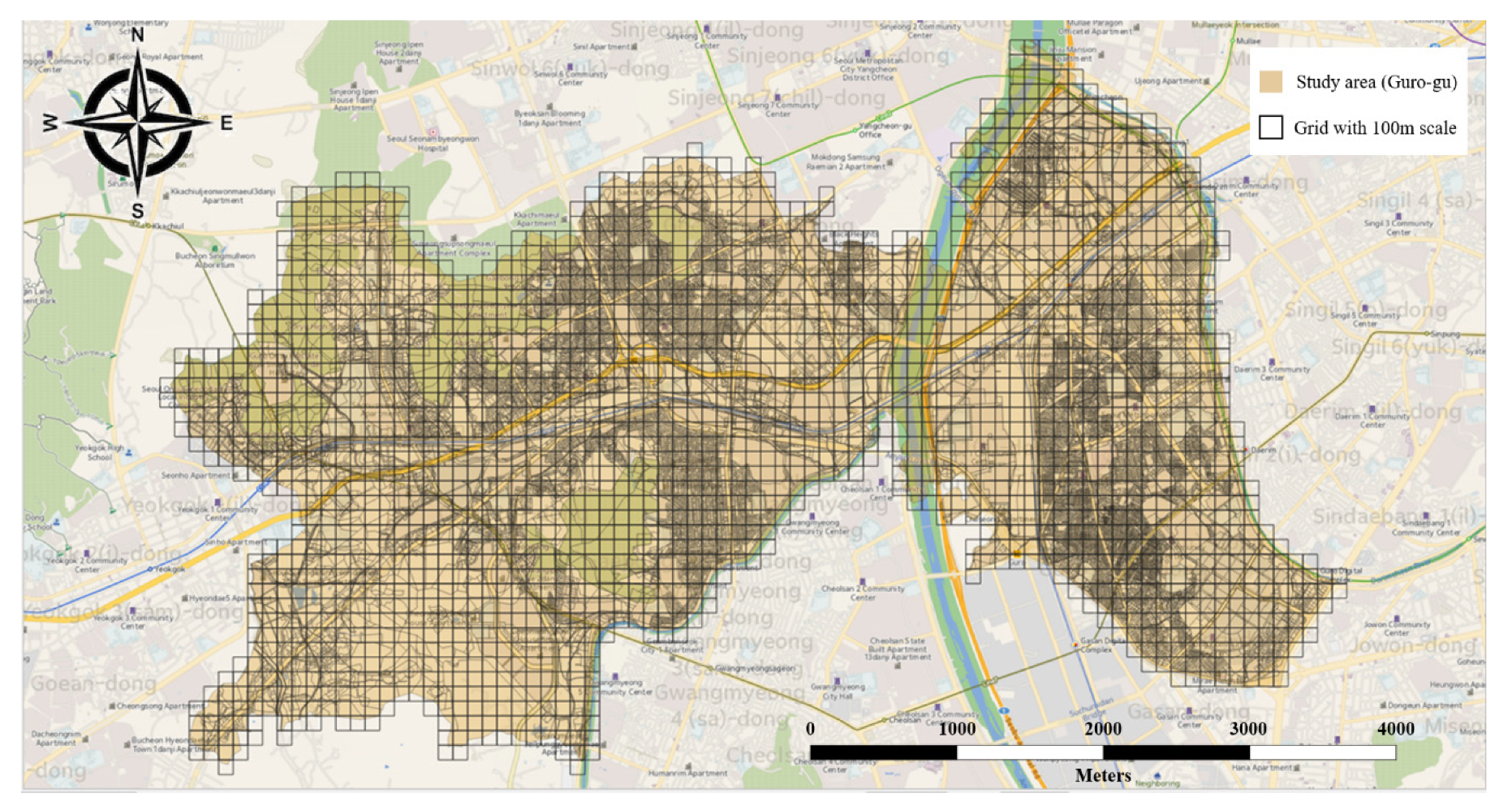
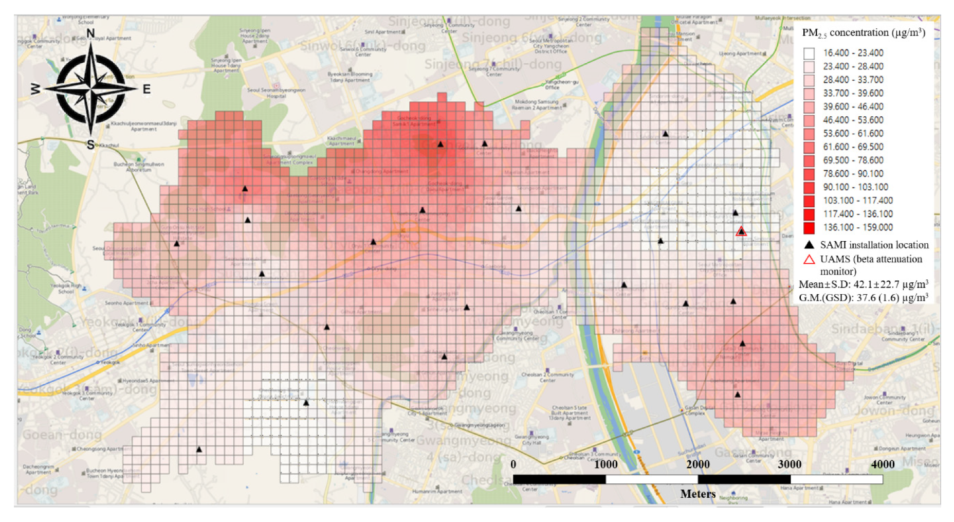
2.1. Subject Area
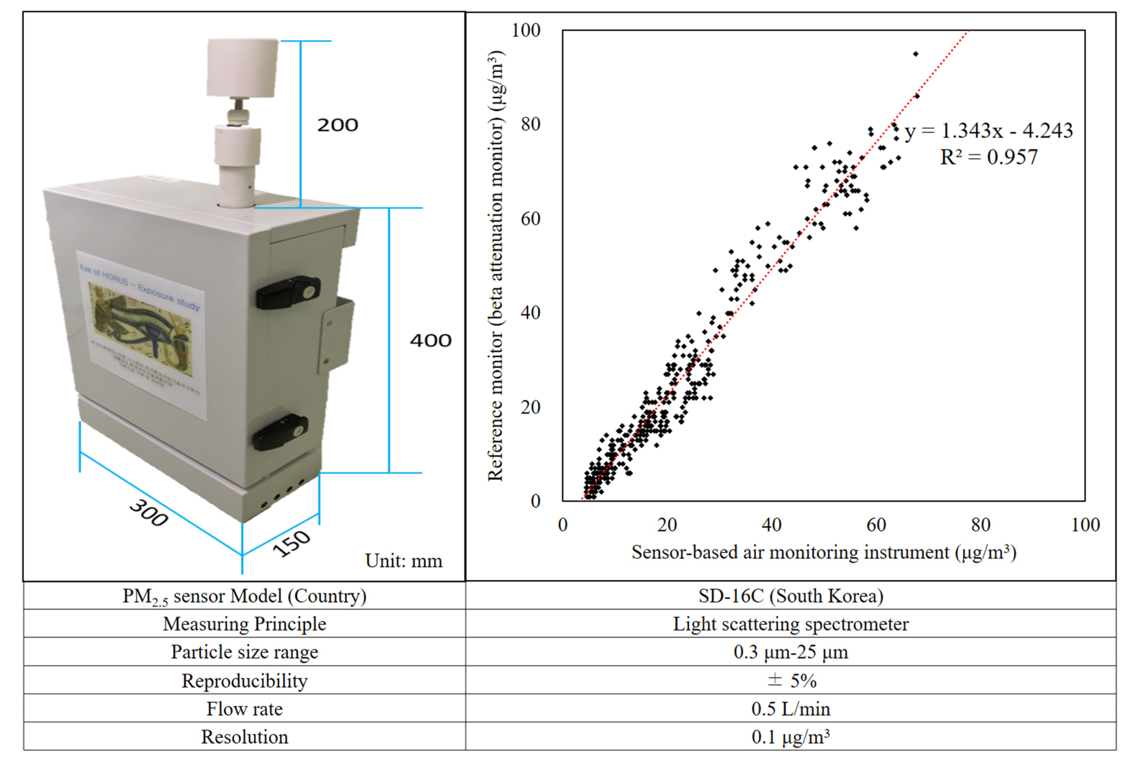
2.2. Indoor and Outdoor Exposure Model
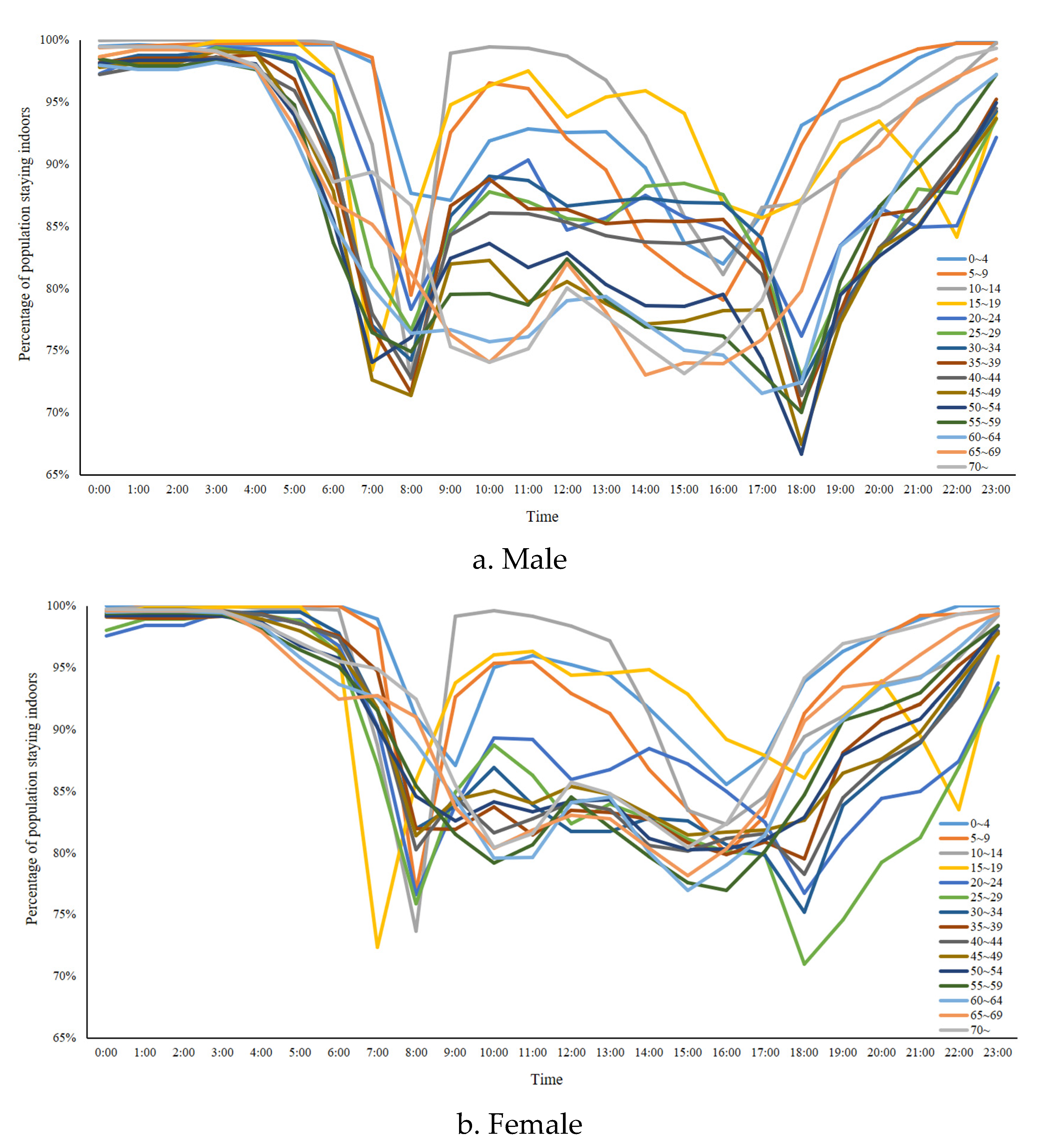
2.3. Population Distribution
2.4. Population Exposure
3. Results
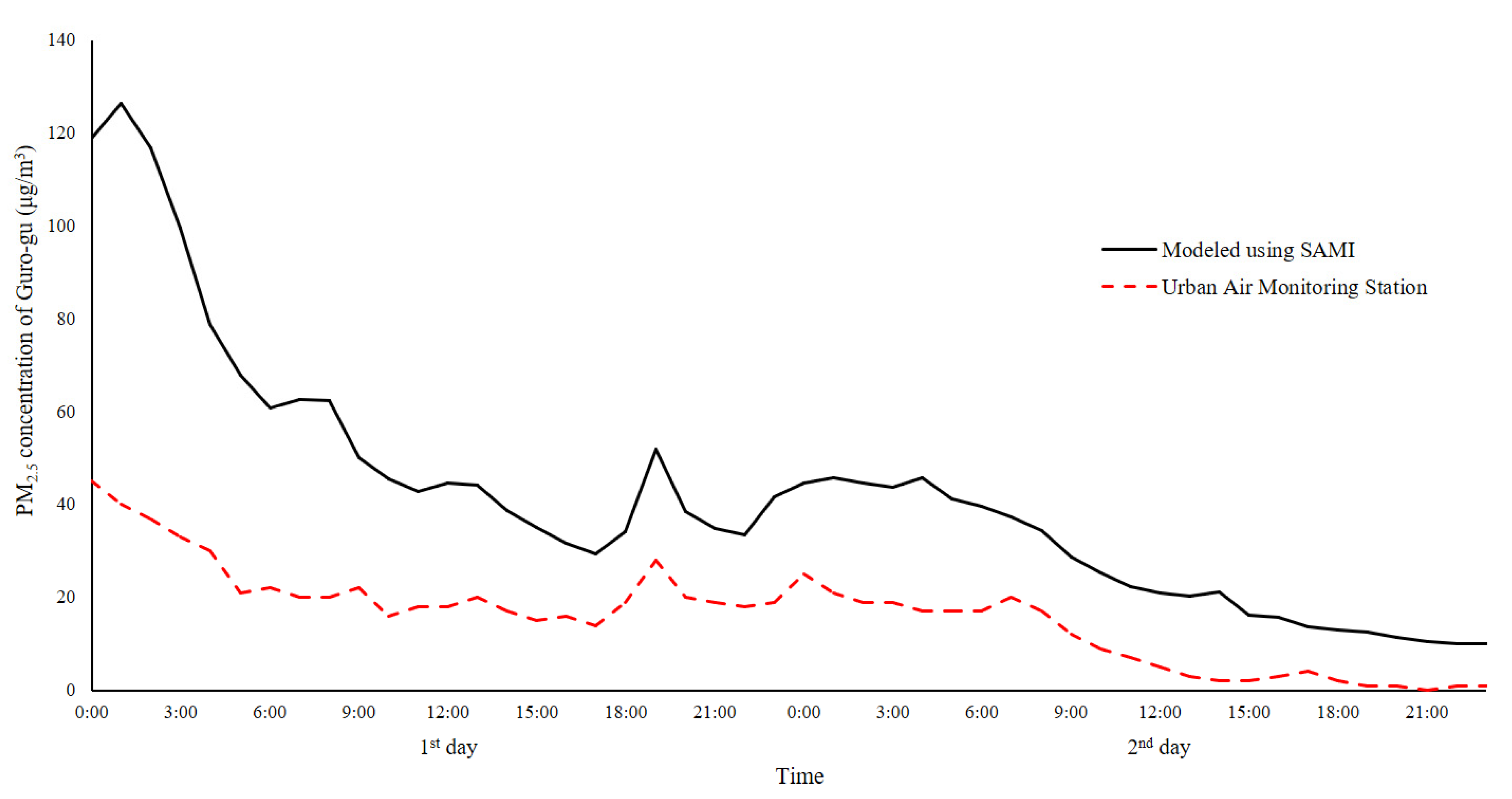
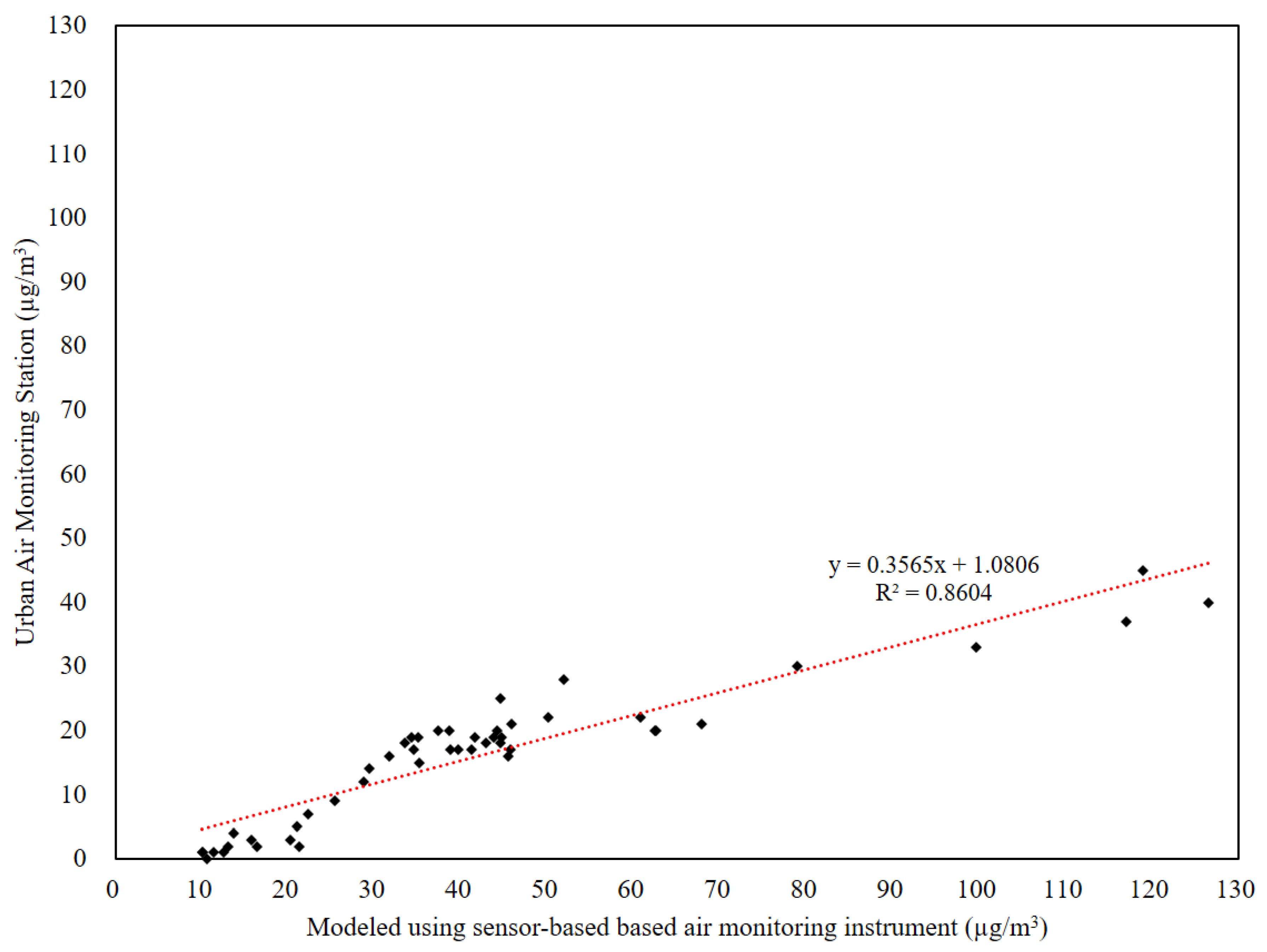
3.1. Indoor and Outdoor Exposure Model
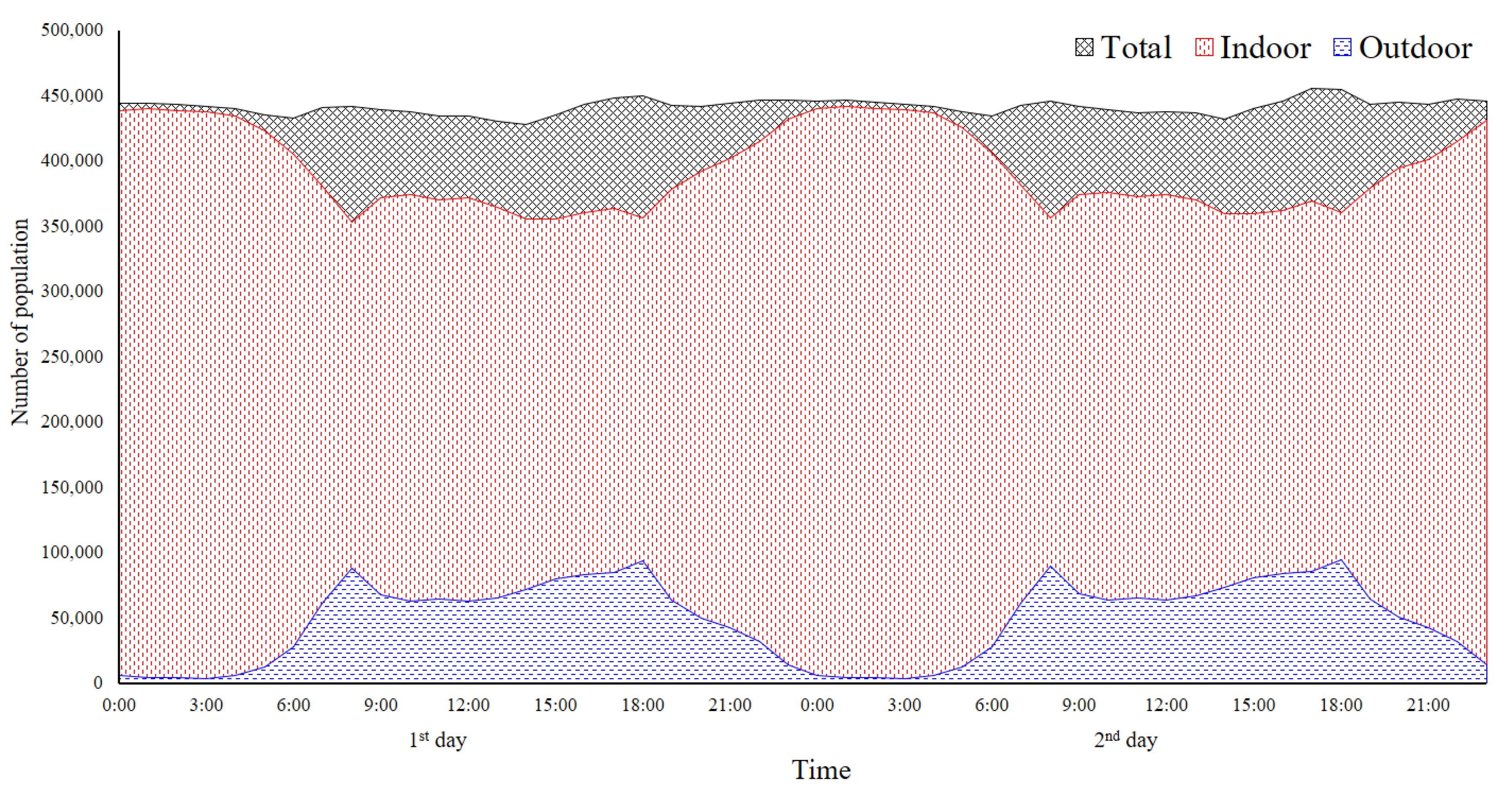
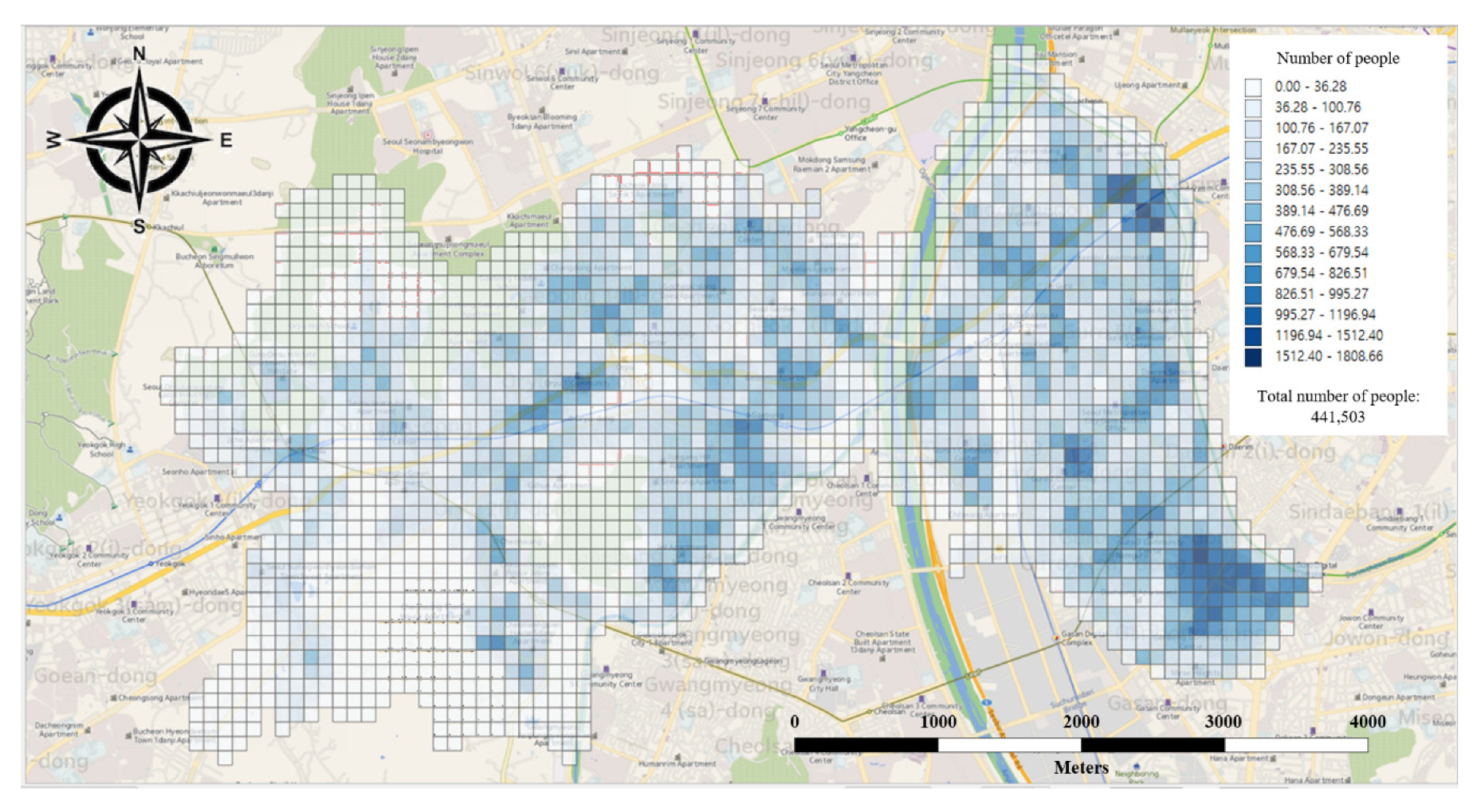
3.2. Population Distribution
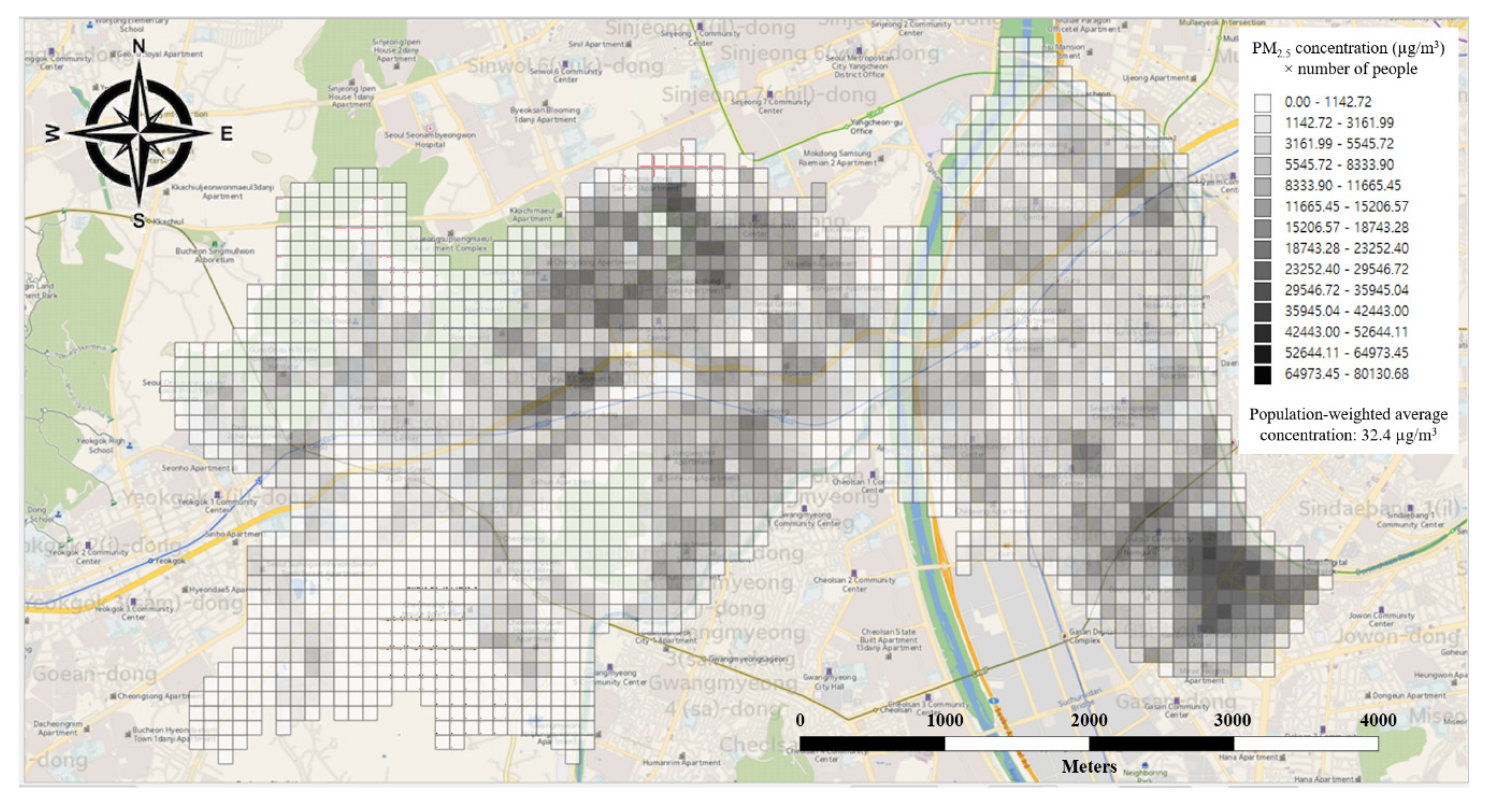
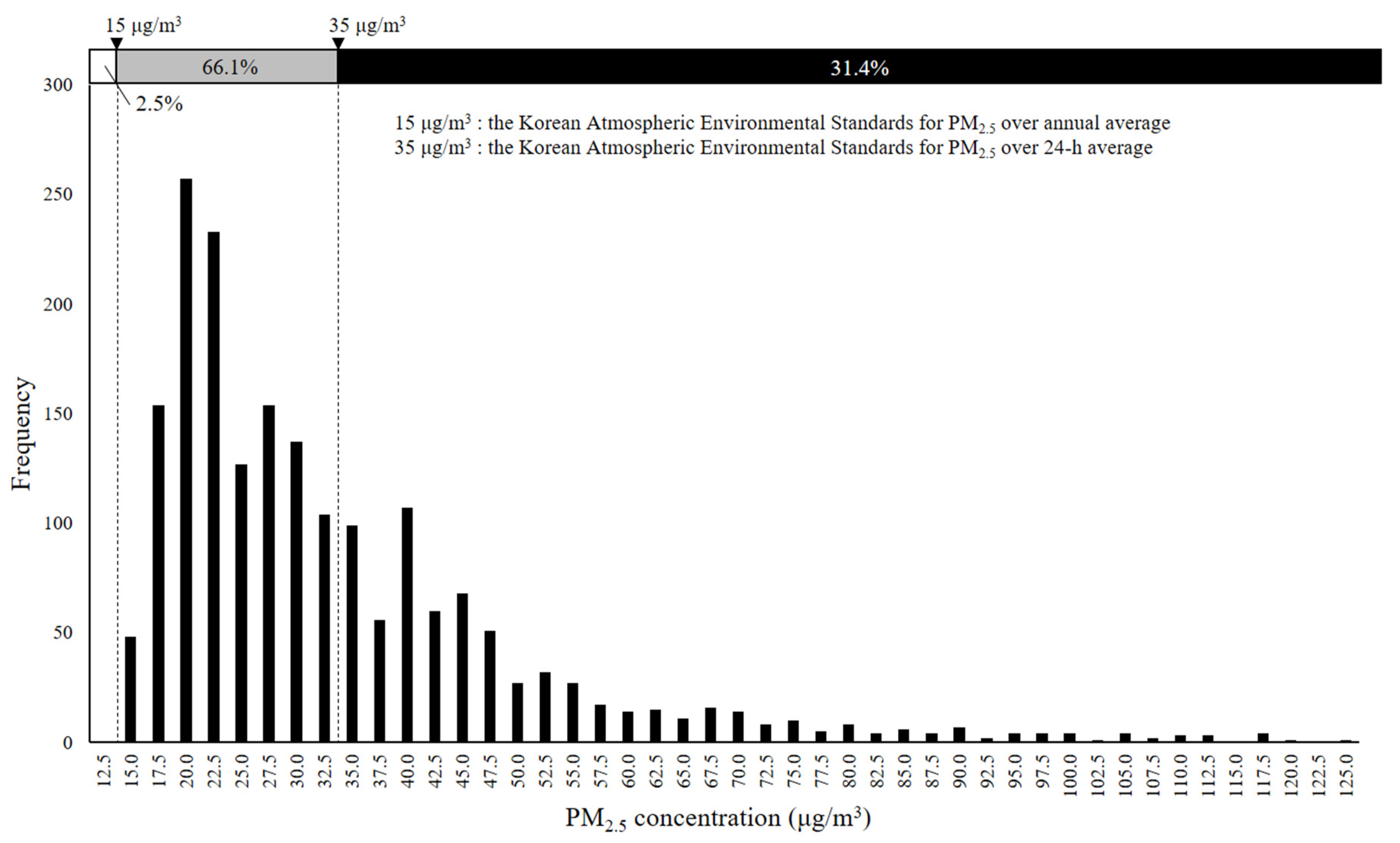
3.3. Population Exposure
4. Discussion
5. Conclusions
Supplementary Materials
Author Contributions
Funding
Acknowledgments
Conflicts of Interest
References
- IARC. IARC Monographs on the Evaluation of Carcinogenic Risks to Humans Volume 109; Müller, k., Ed.; International Agency for Research on Cancer: Lyon, France, 2016; ISBN 978-92-832-0147-2. [Google Scholar]
- WHO Health effects of particulate matter; WHO Regional Office for Europe: Copenhagen, Denmark, 2013; ISBN 978 92 890 0001 7.
- Di, Q.; Wang, Y.; Zanobetti, A.; Wang, Y.; Koutrakis, P.; Choirat, C.; Dominici, F.; Schwartz, J.D. Air pollution and mortality in the medicare population. N. Engl. J. Med. 2017, 376, 2513–2522. [Google Scholar] [CrossRef]
- Burke, J.M.; Zufall, M.J.; Özkaynak, H. A population exposure model for particulate matter: Case study results for PM2.5 in Philadelphia, PA. J. Expo. Anal. Environ. Epidemiol. 2001, 11, 470–489. [Google Scholar] [CrossRef] [Green Version]
- Vaidyanathan, A.; Dimmick, W.F.; Kegler, S.R.; Qualters, J.R. Statistical air quality predictions for public health surveillance: Evaluation and generation of county level metrics of PM2.5 for the environmental public health tracking network. Int. J. Health Geogr. 2013, 12, 1–13. [Google Scholar] [CrossRef] [Green Version]
- Owodunni, T.; Close, R.; Muhammad, U.; Loon, B.; Behbod, B.; Crabbe, H.; Meara, J.; Oliver, I.; Kamanyire, R.; Verne, J.; et al. Developing an Environmental Public Health Surveillance System for England. Available online: https://ehp.niehs.nih.gov/doi/abs/10.1289/isee.2016.4673 (accessed on 15 January 2020).
- Gianicolo, E.; Bruni, A.; Serinelli, M. Environmental Health Surveillance. CNR Environ. Heal. Inter-departmental Proj. 2008, 16. [Google Scholar]
- Joas, A.; Schöpel, M.; David, M.; Casas, M.; Koppen, G.; Esteban, M.; Knudsen, L.E.; Vrijheid, M.; Schoeters, G.; Calvo, A.C.; et al. Environmental health surveillance in a future European health information system. Arch. Public Heal. 2018, 76, 27. [Google Scholar] [CrossRef] [Green Version]
- Kaivonen, S.; Ngai, E.C.H. Real-time air pollution monitoring with sensors on city bus. Digit. Commun. Networks 2019, 6, 23–30. [Google Scholar] [CrossRef]
- Williams, R.; Duvall, R.; Kilaru, V.; Hagler, G.; Hassinger, L.; Benedict, K.; Rice, J.; Kaufman, A.; Judge, R.; Pierce, G.; et al. Deliberating performance targets workshop: Potential paths for emerging PM2.5 and O3 air sensor progress. Atmos. Environ. X 2019, 2, 100031. [Google Scholar] [CrossRef]
- Chen, B.; Song, Y.; Jiang, T.; Chen, Z.; Huang, B.; Xu, B. Real-time estimation of population exposure to PM2.5 using mobile- and station-based big data. Int. J. Environ. Res. Public Health 2018, 15. [Google Scholar] [CrossRef] [Green Version]
- Dewulf, B.; Neutens, T.; Lefebvre, W.; Seynaeve, G.; Vanpoucke, C.; Beckx, C.; Van de Weghe, N. Dynamic assessment of exposure to air pollution using mobile phone data. Int. J. Health Geogr. 2016, 15. [Google Scholar] [CrossRef] [Green Version]
- Schneider, P.; Castell, N.; Vogt, M.; Dauge, F.R.; Lahoz, W.A.; Bartonova, A. Mapping urban air quality in near real-time using observations from low-cost sensors and model information. Environ. Int. 2017, 106, 234–247. [Google Scholar] [CrossRef]
- DeFelice, T.P. Relationship between temporal anomalies in PM2.5 concentrations and reported influenza/influenza-like illness activity. Heliyon 2020, 6, e04726. [Google Scholar] [CrossRef]
- Chen, Y.; Wild, O.; Conibear, L.; Ran, L.; He, J.; Wang, L.; Wang, Y. Local characteristics of and exposure to fine particulate matter (PM2.5) in four indian megacities. Atmos. Environ. X 2020, 5, 100052. [Google Scholar] [CrossRef]
- Huang, L.; Zhou, L.; Chen, J.; Chen, K.; Liu, Y.; Chen, X.; Tang, F. Acute effects of air pollution on influenza-like illness in Nanjing, China: A population-based study. Chemosphere 2016, 147, 180–187. [Google Scholar] [CrossRef]
- Zhang, A.; Qi, Q.; Jiang, L.; Zhou, F.; Wang, J. Population Exposure to PM2.5 in the Urban Area of Beijing. PLoS One 2013, 8, e63486. [Google Scholar] [CrossRef] [Green Version]
- Picornell, M.; Ruiz, T.; Borge, R.; García-Albertos, P.; de la Paz, D.; Lumbreras, J. Population dynamics based on mobile phone data to improve air pollution exposure assessments. J. Expo. Sci. Environ. Epidemiol. 2019, 29, 278–291. [Google Scholar] [CrossRef]
- Ivy, D.; Mulholland, J.A.; Russell, A.G. Development of ambient air quality population-weighted metrics for use in time-series health studies. J. Air Waste Manag. Assoc. 2008, 58, 711–720. [Google Scholar] [CrossRef] [Green Version]
- Yoo, S.K.; Kim, B.Y. A decision-making model for adopting a cloud computing system. Sustain. 2018, 10, 2952. [Google Scholar] [CrossRef] [Green Version]
- Bo, M.; Salizzoni, P.; Clerico, M.; Buccolieri, R. Assessment of indoor-outdoor particulate matter air pollution: A review. Atmosphere (Basel). 2017, 8. [Google Scholar] [CrossRef] [Green Version]
- Park, J.; Ryu, H.; Kim, E.; Choe, Y.; Heo, J.; Lee, J.; Cho, S.H.; Sung, K.; Cho, M.; Yang, W. Assessment of PM2.5 population exposure of a community using sensor-based air monitoring instruments and similar time-activity groups. Atmos. Pollut. Res. 2020, 11, 1971–1981. [Google Scholar] [CrossRef]
- Park, J.; Kim, E.; Choe, Y.; Ryu, H.; Kim, S. Indoor to Outdoor Ratio of Fine Particulate Matter by Time of the Day in House According to Time-activity Patterns. J. Environ. Health Sci. 2020, 46, 504–512. [Google Scholar]
- Yoon, H.; Yoo, S.K.; Seo, J.; Kim, T.; Kim, P.; Kim, P.J.; Park, J.; Heo, J.; Yang, W. Development of General Exposure Factors for Risk Assessment in Korean Children. Int. J. Environ. Res. Public Health 2020, 17, 1–14. [Google Scholar] [CrossRef] [Green Version]
- Yang, W.; Song, Y.; Shin, K.; H, L. Study on the Improvement of Exposure Factors of Korean Adults on Risk Assessment; National Institute of Environmental Research: Incheon, Korea, 2018. [Google Scholar]
- Fu, X.; Zhu, X.; Jiang, Y.; Zhang, J. (Jim); Wang, T.; Jia, C. Centralized outdoor measurements of fine particulate matter as a surrogate of personal exposure for homogeneous populations. Atmos. Environ. 2019, 204, 110–117. [Google Scholar] [CrossRef]
- Taştan, M.; Gökozan, H. Real-time monitoring of indoor air quality with internet of things-based e-nose. Appl. Sci. 2019, 9, 3435. [Google Scholar] [CrossRef]
- Kumar, P.; Morawska, L.; Martani, C.; Biskos, G.; Neophytou, M.; Di Sabatino, S.; Bell, M.; Norford, L.; Britter, R. The rise of low-cost sensing for managing air pollution in cities. Environ. Int. 2015, 75, 199–205. [Google Scholar] [CrossRef] [Green Version]
- Castell, N.; Dauge, F.R.; Schneider, P.; Vogt, M.; Lerner, U.; Fishbain, B.; Broday, D.; Bartonova, A. Can commercial low-cost sensor platforms contribute to air quality monitoring and exposure estimates? Environ. Int. 2017, 99, 293–302. [Google Scholar] [CrossRef]
- Tagle, M.; Rojas, F.; Reyes, F.; Vásquez, Y.; Hallgren, F.; Lindén, J.; Kolev, D.; Watne, Å.K.; Oyola, P. Field performance of a low-cost sensor in the monitoring of particulate matter in Santiago, Chile. Environ. Monit. Assess. 2020, 192. [Google Scholar] [CrossRef] [Green Version]
- Lin, Y.C.; Chi, W.J.; Lin, Y.Q. The improvement of spatial-temporal resolution of PM2.5 estimation based on micro-air quality sensors by using data fusion technique. Environ. Int. 2020, 134, 105305. [Google Scholar] [CrossRef]
- Madakam, S.; Ramaswamy, R.; Tripathi, S. Internet of Things (IoT): A Literature Review. J. Comput. Commun. 2015, 03, 164–173. [Google Scholar] [CrossRef] [Green Version]
- Zanella, A.; Bui, N.; Castellani, A.; Vangelista, L.; Zorzi, M. Internet of things for smart cities. IEEE Internet Things J. 2014, 1, 22–32. [Google Scholar] [CrossRef]
- Khatoon, N.; Roy, S.; Pranav, P. A Survey on Applications of Internet of Things in Healthcare. Intell. Syst. Ref. Libr. 2020, 180, 89–106. [Google Scholar] [CrossRef]
- Moschandreas, D.J.; Watson, J.; D’Abreton, P.; Scire, J.; Zhu, T.; Klein, W.; Saksena, S. Chapter three: Methodology of exposure modeling. Chemosphere 2002, 49, 923–946. [Google Scholar] [CrossRef]
- Ayturan, Y.A.; Ayturan, Z.C.; Altun, H.O. Air Pollution Modelling with Deep Learning: A Review. Int. J. Environ. Pollut. Environ. Model. 2018, 1, 58–62. [Google Scholar]
- Yang, W.; Park, J.; Cho, M.; Lee, C.; Lee, J.; Lee, C. Environmental health surveillance system for a population using advanced exposure assessment. Toxics 2020, 8, 74. [Google Scholar] [CrossRef] [PubMed]
- Goyal, R.; Kumar, P. Indoor-outdoor concentrations of particulate matter in nine microenvironments of a mix-use commercial building in megacity Delhi. Air Qual. Atmos. Heal. 2013, 6, 747–757. [Google Scholar] [CrossRef] [Green Version]
- Zuo, J.X.; Ji, W.; Ben, Y.J.; Hassan, M.A.; Fan, W.H.; Bates, L.; Dong, Z.M. Using big data from air quality monitors to evaluate indoor PM2.5 exposure in buildings: Case study in Beijing. Environ. Pollut. 2018, 240, 839–847. [Google Scholar] [CrossRef] [PubMed]
- Massey, D.; Kulshrestha, A.; Masih, J.; Taneja, A. Seasonal trends of PM10, PM5.0, PM2.5 & PM1.0 in indoor and outdoor environments of residential homes located in North-Central India. Build. Environ. 2012, 47, 223–231. [Google Scholar] [CrossRef]
- Ji, W.; Zhao, B. Contribution of outdoor-originating particles, indoor-emitted particles and indoor secondary organic aerosol (SOA) to residential indoor PM2.5 concentration: A model-based estimation. Build. Environ. 2015, 90, 196–205. [Google Scholar] [CrossRef]
- Mannucci, P.M.; Franchini, M. Health effects of ambient air pollution in developing countries. Int. J. Environ. Res. Public Health 2017, 14, 1–8. [Google Scholar] [CrossRef]
- Chen, C.; Zhao, B. Review of relationship between indoor and outdoor particles: I/O ratio, infiltration factor and penetration factor. Atmos. Environ. 2011, 45, 275–288. [Google Scholar] [CrossRef]
- Benammar, M.; Abdaoui, A.; Ahmad, S.H.M.; Touati, F.; Kadri, A. A modular IoT platform for real-time indoor air quality monitoring. Sensors (Switzerland) 2018, 18, 1–18. [Google Scholar] [CrossRef] [Green Version]
- Wei, W.; Ramalho, O.; Malingre, L.; Sivanantham, S.; Little, J.C.; Mandin, C. Machine learning and statistical models for predicting indoor air quality. Indoor Air 2019, 29, 704–726. [Google Scholar] [CrossRef] [PubMed]
- EPA Consolidated Human Activity Database (CHAD) for Use in Human Exposure and Health Studies and Predictive Models. Available online: https://www.epa.gov/healthresearch/consolidated-human-activity-database-chad-use-human-exposure-and-health-studies-and (accessed on 15 January 2020).
- Su, J.G.; Apte, J.S.; Lipsitt, J.; Garcia-Gonzales, D.A.; Beckerman, B.S.; de Nazelle, A.; Texcalac-Sangrador, J.L.; Jerrett, M. Populations potentially exposed to traffic-related air pollution in seven world cities. Environ. Int. 2015, 78, 82–89. [Google Scholar] [CrossRef] [PubMed]
- Reis, S.; Seto, E.; Northcross, A.; Quinn, N.W.T.; Convertino, M.; Jones, R.L.; Maier, H.R.; Schlink, U.; Steinle, S.; Vieno, M.; et al. Integrating modelling and smart sensors for environmental and human health. Environ. Model. Softw. 2015, 74, 238–246. [Google Scholar] [CrossRef] [PubMed] [Green Version]
- De Nazelle, A.; Seto, E.; Donaire-Gonzalez, D.; Mendez, M.; Matamala, J.; Nieuwenhuijsen, M.J.; Jerrett, M. Improving estimates of air pollution exposure through ubiquitous sensing technologies. Environ. Pollut. 2013, 176, 92–99. [Google Scholar] [CrossRef] [Green Version]
- Nyhan, M.M.; Kloog, I.; Britter, R.; Ratti, C.; Koutrakis, P. Quantifying population exposure to air pollution using individual mobility patterns inferred from mobile phone data. J. Expo. Sci. Environ. Epidemiol. 2019, 29, 238–247. [Google Scholar] [CrossRef]
- De Nadai, M.; Cardoso, A.; Lima, A.; Lepri, B.; Oliver, N. Strategies and limitations in app usage and human mobility. Sci. Rep. 2019, 9, 1–9. [Google Scholar] [CrossRef] [Green Version]
- Breen, M.; Isakov, V.; Seppanen, C.; Arunachalam, S.; Samet, J.; Devlin, M.; Cascio, W.; Diaz-Sanchez, D.; Tong, H. Development of Smartphone Application for Modeling Personal Exposures to Ambient PM2.5 and Ozone. Environ. Epidemiol. 2019, 3, 41. [Google Scholar] [CrossRef]
- Oh, J.; An, J. Depressive Symptoms, Emotional Aggression, School Adjustment, and Mobile Phone Dependency Among Adolescents with Allergic Diseases in South Korea. J. Pediatr. Nurs. 2019, 47, e24–e29. [Google Scholar] [CrossRef]
- Yin, P.; Brauer, M.; Cohen, A.J.; Wang, H.; Li, J.; Burnett, R.T.; Stanaway, J.D.; Causey, K.; Larson, S.; Godwin, W.; et al. The effect of air pollution on deaths, disease burden, and life expectancy across China and its provinces, 1990–2017: An analysis for the Global Burden of Disease Study 2017. Lancet Planet. Heal. 2020, 4, e386–e398. [Google Scholar] [CrossRef]
- Aunan, K.; Ma, Q.; Lund, M.T.; Wang, S. Population-weighted exposure to PM 2.5 pollution in China: An integrated approach. Environ. Int. 2018, 120, 111–120. [Google Scholar] [CrossRef]
- Huang, G.; Brown, P.E. Population-weighted exposure to air pollution and COVID-19 incidence in Germany. Spat. Stat. 2021, 41, 100480. [Google Scholar] [CrossRef] [PubMed]


| Sex | Age | Indoor (%) | |||||
|---|---|---|---|---|---|---|---|
| Home | Workplace or School | Other House | Restaurant or Bar | Other Indoors | Transport | ||
| Male | 19–24 | 99.86 | 95.18 | 100.00 | 99.25 | 87.87 | 100 |
| 25–34 | 99.97 | 94.98 | 100.00 | 94.24 | 83.91 | ||
| 35–44 | 99.93 | 96.66 | 100.00 | 96.15 | 74.19 | ||
| 45–54 | 99.95 | 95.23 | 100.00 | 96.76 | 50.60 | ||
| 55–64 | 99.82 | 92.77 | 100.00 | 94.92 | 52.57 | ||
| 65–74 | 99.80 | 89.96 | 98.78 | 95.71 | 52.51 | ||
| <75 | 99.46 | 57.14 | 100.00 | 97.87 | 50.86 | ||
| Female | 19–24 | 99.94 | 97.45 | 100.00 | 97.99 | 83.27 | |
| 25–34 | 100 | 98.64 | 100.00 | 92.46 | 32.14 | ||
| 35–44 | 99.95 | 98.02 | 100.00 | 98.41 | 49.04 | ||
| 45–54 | 99.91 | 99.77 | 100.00 | 97.77 | 55.70 | ||
| 55–64 | 99.95 | 95.59 | 100.00 | 99.62 | 55.33 | ||
| 65–74 | 99.82 | 91.58 | 96.88 | 94.12 | 70.64 | ||
| <75 | 99.76 | 100.00 | 100.00 | 100.00 | 59.60 | ||
Publisher’s Note: MDPI stays neutral with regard to jurisdictional claims in published maps and institutional affiliations. |
© 2020 by the authors. Licensee MDPI, Basel, Switzerland. This article is an open access article distributed under the terms and conditions of the Creative Commons Attribution (CC BY) license (http://creativecommons.org/licenses/by/4.0/).
Share and Cite
Park, J.; Jo, W.; Cho, M.; Lee, J.; Lee, H.; Seo, S.; Lee, C.; Yang, W. Spatial and Temporal Exposure Assessment to PM2.5 in a Community Using Sensor-Based Air Monitoring Instruments and Dynamic Population Distributions. Atmosphere 2020, 11, 1284. https://doi.org/10.3390/atmos11121284
Park J, Jo W, Cho M, Lee J, Lee H, Seo S, Lee C, Yang W. Spatial and Temporal Exposure Assessment to PM2.5 in a Community Using Sensor-Based Air Monitoring Instruments and Dynamic Population Distributions. Atmosphere. 2020; 11(12):1284. https://doi.org/10.3390/atmos11121284
Chicago/Turabian StylePark, Jinhyeon, Wondeuk Jo, Mansu Cho, Jeongil Lee, Hunjoo Lee, SungChul Seo, Chulmin Lee, and Wonho Yang. 2020. "Spatial and Temporal Exposure Assessment to PM2.5 in a Community Using Sensor-Based Air Monitoring Instruments and Dynamic Population Distributions" Atmosphere 11, no. 12: 1284. https://doi.org/10.3390/atmos11121284