
Features Exploration from Datasets Vision in Air Quality Prediction Domain


Institute of New Imaging Technologies (INIT), Universitat Jaume I, Avinguda Vicente Sos Baynat s/n, 12071 Castelló de la Plana, Spain
*
Author to whom correspondence should be addressed.
Atmosphere 2021, 12(3), 312; https://doi.org/10.3390/atmos12030312
Submission received: 5 January 2021
/
Revised: 21 February 2021
/
Accepted: 23 February 2021
/
Published: 28 February 2021
(This article belongs to the Special Issue Advances in Air Quality Data Analysis and Modeling)
Abstract
:Air pollution and its consequences are negatively impacting on the world population and the environment, which converts the monitoring and forecasting air quality techniques as essential tools to combat this problem. To predict air quality with maximum accuracy, along with the implemented models and the quantity of the data, it is crucial also to consider the dataset types. This study selected a set of research works in the field of air quality prediction and is concentrated on the exploration of the datasets utilised in them. The most significant findings of this research work are: (1) meteorological datasets were used in 94.6% of the papers leaving behind the rest of the datasets with a big difference, which is complemented with others, such as temporal data, spatial data, and so on; (2) the usage of various datasets combinations has been commenced since 2009; and (3) the utilisation of open data have been started since 2012, 32.3% of the studies used open data, and 63.4% of the studies did not provide the data.
1. Introduction
According to the United Nations (UN) in 2018, more than 55% of the world’s population lives in urban areas. The trend shows that by 2050 urban population will increase until 68%; particularly compared to other regions, the urban population will grow faster in Asia and Africa, considering that these regions have more rural population [1]. Among the positive effects, such as better employment and education opportunities, enhanced healthcare system, greater access to social services, urbanisation also has negative consequences being a cause of air pollution or the increased demands on resources, among others. According to the World Health Organisation (WHO), every year, more than seven million persons die because of this problem or related to that [2].
It is very important to understand which pollutants are considered when determining air quality, and how to calculate and represent air quality indicators. Regarding the pollutants, they form from natural and anthropogenic sources. The WHO identifies the following pollutants as having serious impacts: particulate matter with diameter less than 2.5 micrometers (PM2.5), particulate matter with diameter less than 10 micrometers (PM10), nitrogen oxide (NOx), ground-level ozone (O3) and sulfur dioxide (SO2) [3]. Depending on the region and the presence of predominant pollutants, it is proposed to use different indices for calculating air quality, for example, the United States Environmental Protection Agency (EPA) Air Quality Index (AQI), the Canada Air Quality Health Index (AQHI), Common Air Quality Index (CAQI) or Daily Air Quality Index (DAQI), among others.
Information about air quality prediction can prompt authorities and decision-makers to apply protective measures in order to reduce air pollution, and this knowledge helps citizens to organise their daily activities by escaping high polluted areas [4,5]. In order to predict air quality more accurately, it is important to consider external factors that influence air quality and include them as input to run models. As an example of those external factors are precipitation, wind direction, traffic intensity or population density, among others [6,7,8,9]. It should also be emphasised the effect to publish this kind of data as open data, which existence is beneficial both for government and for citizens. The availability of open data have an impact in many areas, such as an increase of transparency, improvement of efficiency and effectiveness of government services, empowerment of citizens, engagement and participation of citizens in governance [10,11]. At the same time, these data can be used by researchers as real inputs to run their models in research works.
Taking the aspects mentioned above into account, the main goal of this manuscript is to analyse and synthesise studies related to air quality prediction using Machine Learning (ML) technologies, and find out: (1) What types of datasets are used to improve air quality predictions? (2) What characteristics of the dataset are important for efficient and effective air quality forecasting? and (3) Which features are the most used to define ML models? We believe that this work can be useful for other new works in the field of air quality prediction. Furthermore, considering the scale of the scope in which the topic may be addressed, it should be noted that the perspective of this work is based on data science, and how the obtained results can be used to start a new study to predict air quality in a certain area.
2. Methods
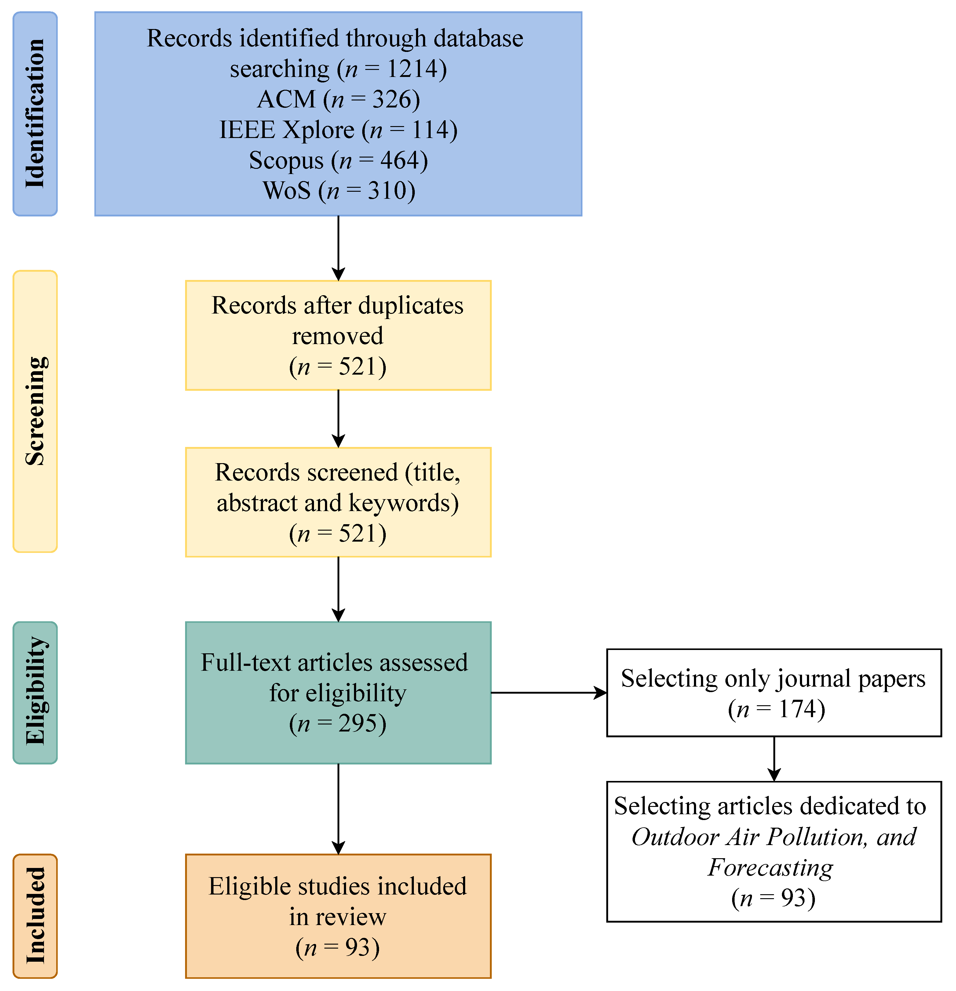
To achieve the central goals for which this study is targeted, we used the Preferred Reporting Items for Systematic Reviews and Meta-Analyses (PRISMA) [12] in order to select relevant papers. Those papers were queried in Association for Computing Machinery (ACM), IEEE Xplore, Scopus and Web of Science (WoS) databases using the following query: (“machine learning”) AND (“prediction” OR “forecast”) AND (“air quality” OR “air pollution”), which was being applied to title, abstract and keywords. At the first stage, it was selected all papers published until 28 September 2020 (search date) and the result was 1214 papers in total. Then duplicated and non-empirical manuscripts were removed. Afterwards, based on the inclusion/exclusion criteria listed in Table 1, screening of title, abstract and keywords, and full-text assessment were implemented. Later, the manuscripts set was filtered by focusing on several aspects. Mainly the main emphasis was to select papers concentrated on forecasting models of outdoor air pollution, which analyses were performed applying ML technologies. Another essential point was to consider the type of datasets, which assumed that in addition to air quality data, the studies should also include different datasets, such as meteorological, spatial or traffic, among others. It also should be mentioned that only journal papers were included in the final set, which has 93 items. After reviewing those papers, the key features were extracted, which are presented in detail in the next section. The described workflow of the selection procedure of the relevant studies is illustrated in Figure 1.
3. Results and Discussion
After analysing the manuscripts set the main objective results, the exploration and observation based on those obtained results are introduced at this stage. The following essential components of the selected studies were extracted, and the result is summarised in Table A1 in Appendix A: Year, Case Study, Prediction Target, Dataset Type, Data Rate, Period (Days), Open Data, Algorithm, Time Granularity and Evaluation Metric.
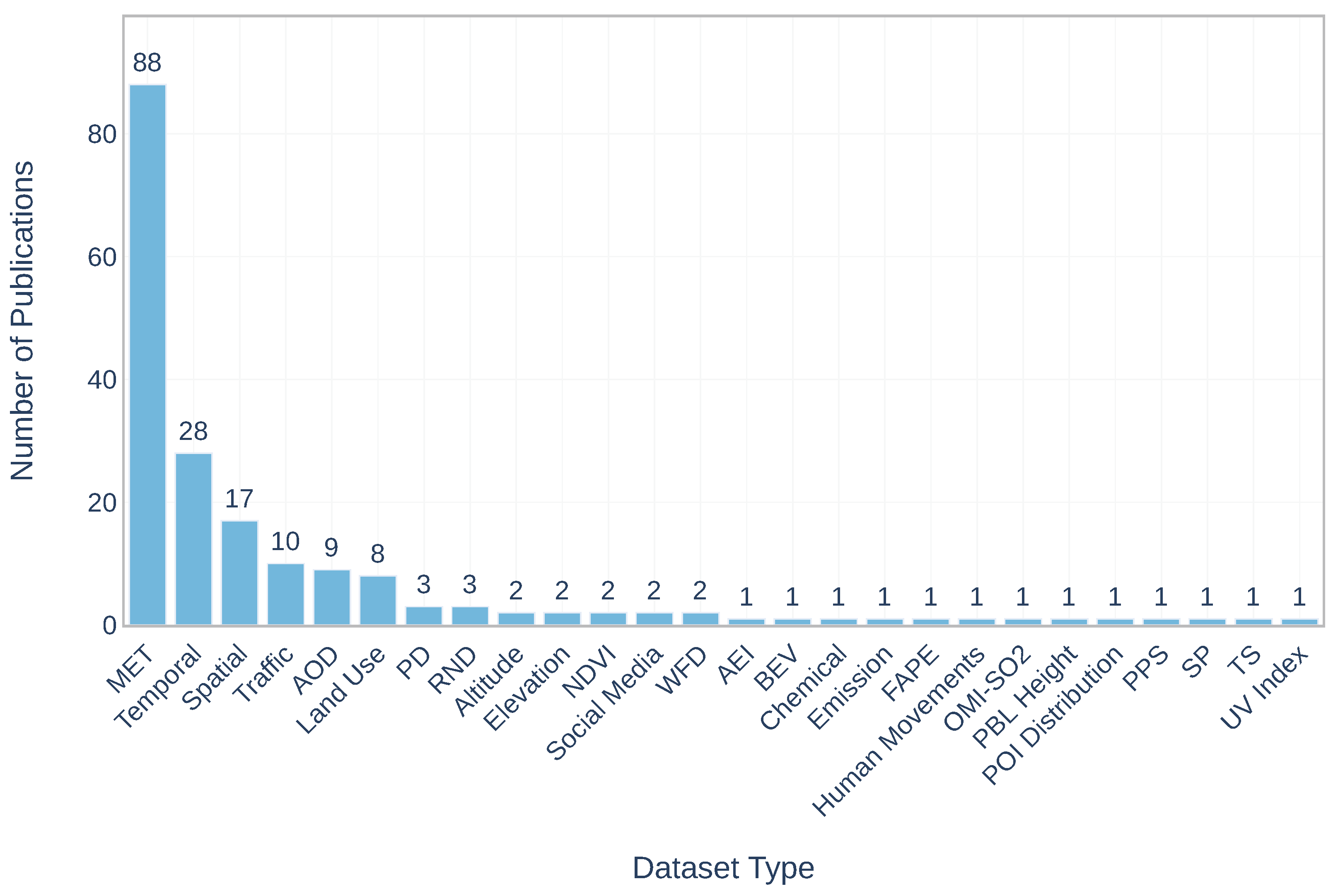
Dataset Type: after examining the selected papers, the following dataset types were extracted (Figure 2): ‘MET’: meteorological data, ‘Spatial’: topographical characteristics, the locations of the stations, ‘Temporal’: includes the day of the month, day of the week, the hour of the day, ‘AOD’: aerosol optical depth, ‘Social Media’: microblog data, ‘Traffic’, ‘PBL Height’: planetary boundary layer height, ‘Land Use’, ‘BEV’: built environment variables, ‘UV Index’: ultraviolet index, ‘SP’: sound pressure, ‘PD’: population density, ‘Human Movements’: floating population and estimated traffic volume, ‘Altitude’, ‘OMI-SO2’: satellite-retrieved SO2 from Ozone Monitoring Instrument-SO2, ‘PPS’: pollution point source, ‘TS’: transportation source, ‘WFD’: weather forecast data, ‘POI Distribution’: point of interest distribution, ‘FAPE’: factory air pollution emission, ‘RND’: road network distribution, ‘Elevation’, ‘AEI’: anthropogenic emission inventory, ‘NDVI’: normalized difference vegetation index, ‘Chemical’: chemical component forecast data (organic carbon, black carbon, sea salt, etc.), ‘Emission’.
From Figure 2 it can be seen that among the 26 dataset types meteorological data is the most used dataset, appearing in eighty-eight publications. The next relatively more frequent dataset types are ‘Temporal’, ‘Spatial’, ‘Traffic’, ‘AOD’ and ‘Land Use’ datasets.
Figure 2 shows the number of publications for each dataset type; however, it is also very important to see the number of publications for dataset combinations. From the dataset types mentioned above, thirty combinations were formed and used in the publications. Table 2 shows the number of publications for each dataset combinations. The most detected combination is meteorological data jointly only with air quality data, appearing in forty-five papers. It should be noted that there are twenty-three datasets combinations, each of them appears only in one publication, so they are combined as Others for the convenience of further analysis.
To find out dataset features used in each research work, each component of Table A1 in Appendix A was observed in terms of dataset types, and the results of the observation are displayed below.
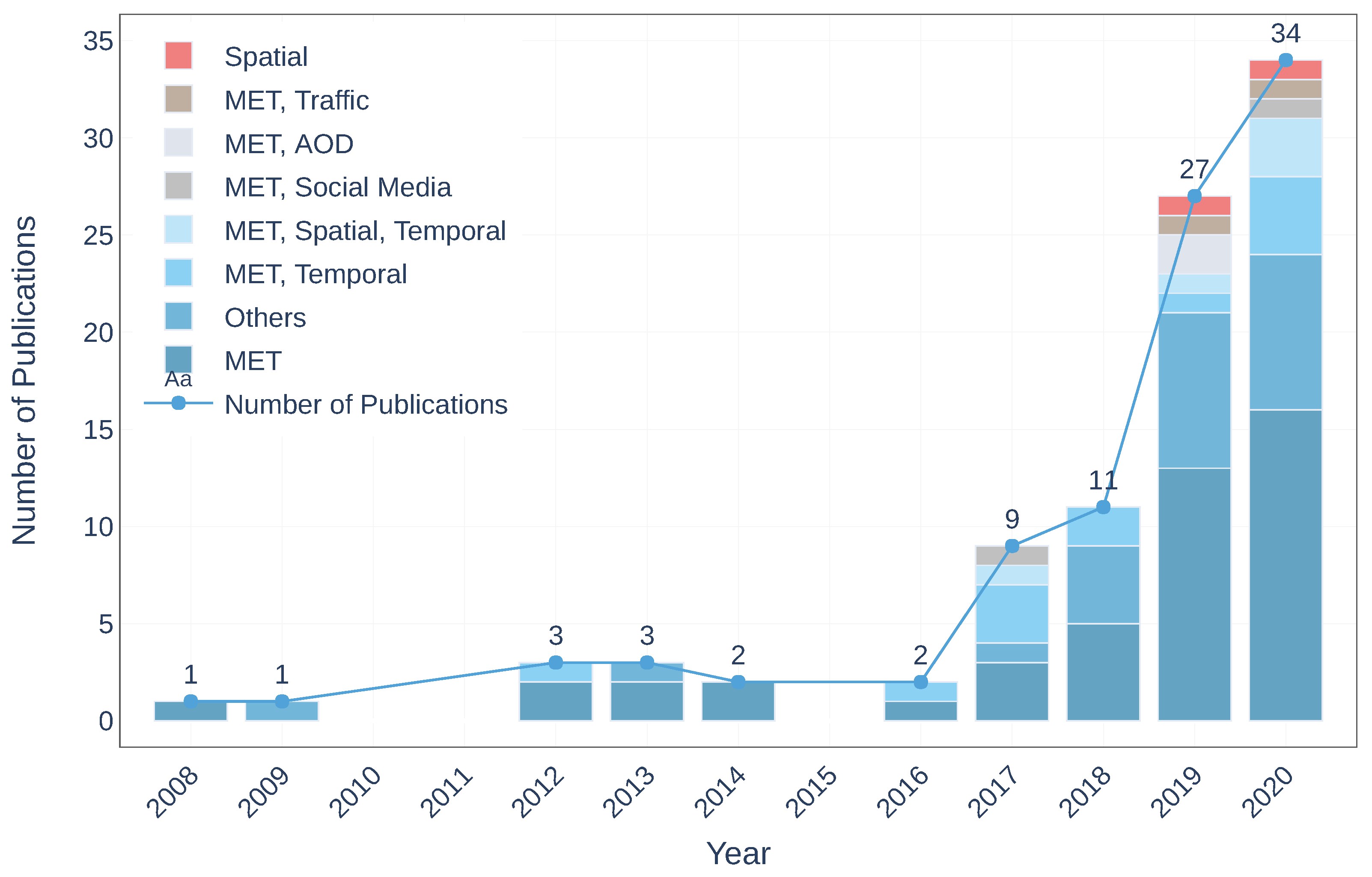
Year: includes years of publications. Figure 3 demonstrates the distribution of the used dataset combinations over the years, mentioning the number of publications of each published year, and it could help to identify the progress throughout the period.
It can be observed that intensive dataset combinations have been applied since 2016, particularly during 2019 and 2020. Only meteorological data were dominant throughout the whole period. The increase in the number of manuscripts can be attributed to the open data movement promoted by the governments [13]. This aspect will be analysed later.
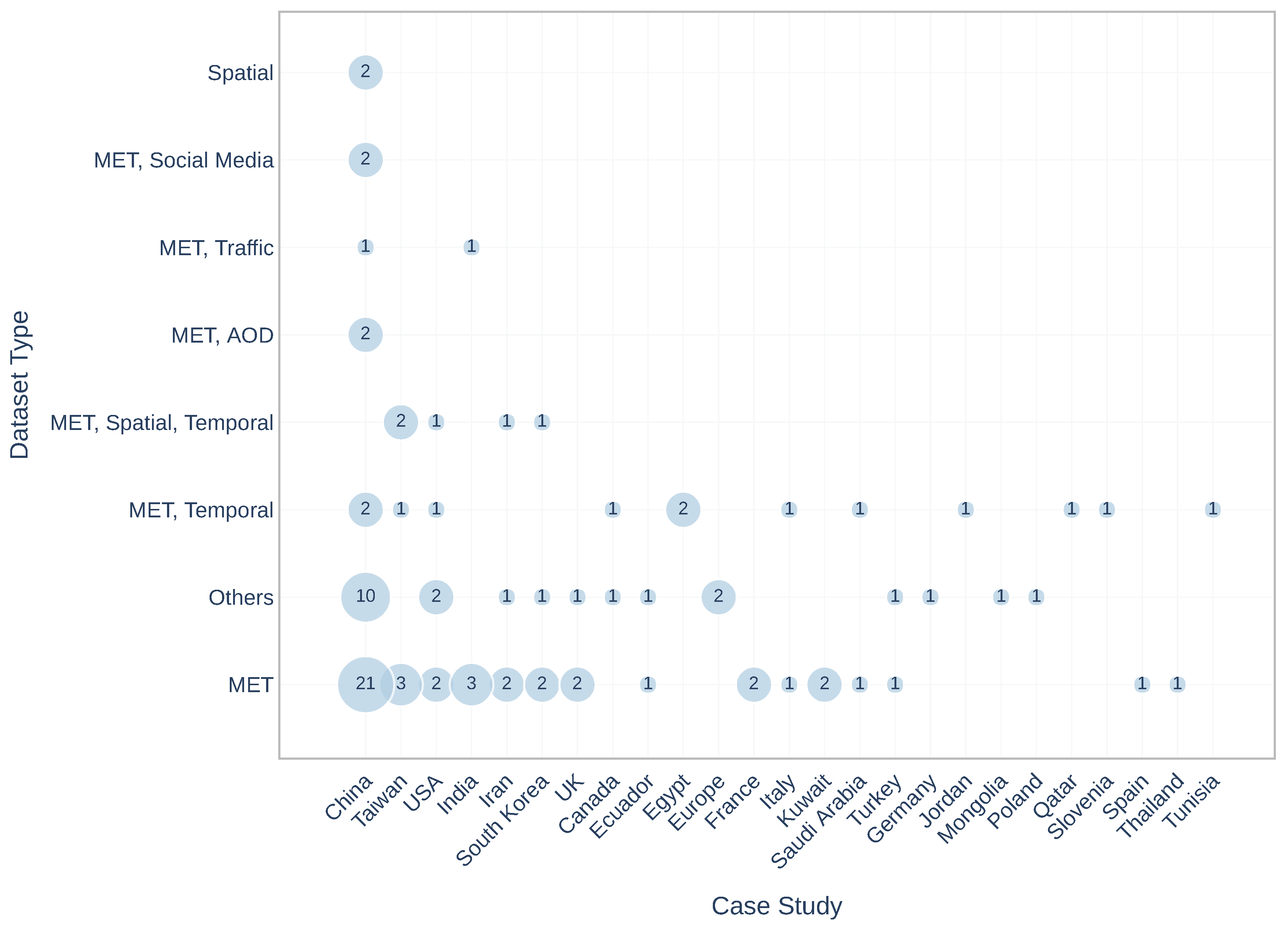
Case Study: are the countries which were served as a case study in the papers. In the majority of the papers (forty) China was a case study. Here is a list of the rest of the countries with the number of publications: USA-six; Taiwan-six; India-four; Iran-four; South Korea-four; UK-three; Canada-two; Ecuador-two; Egypt-two; Europe-two; France-two; Italy-two; Kuwait-two; Saudi Arabia-two; Turkey-two; Germany-one; Jordan-one; Mongolia-one; Poland-one; Qatar-one; Slovenia-one; Spain-one; Thailand-one; and Tunisia-one. Apart from this examination, it will be helpful also to know dataset combinations for each case study. Figure 4 illustrates the distribution of dataset combinations in terms of the case study. As may be noted, China was a case study in the papers with the majority dataset combinations (China with ‘MET’ is the dominant combination (twenty-one papers)), exclusive of ‘MET, Spatial, Temporal’.
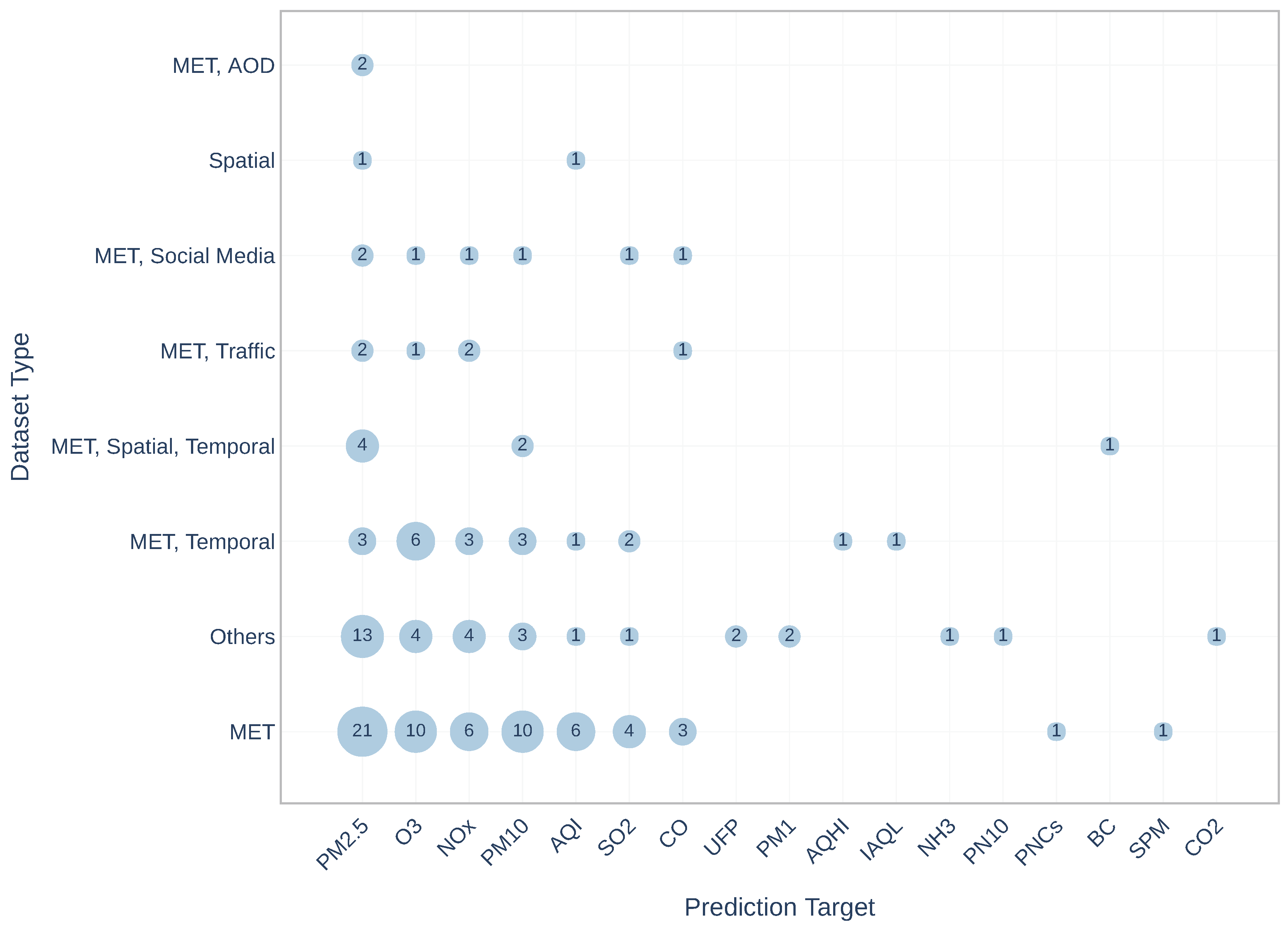
Prediction Target: is the dominant pollutant in a certain area for which prediction different techniques have been performed. In general, seventeen prediction targets were utilised: PM2.5, O3, NOx, PM10, air quality index (AQI), SO2, carbon monoxide (CO), ultrafine particle (UFP or PM0.1), particulate matters less than 0.1 micrometers in diameter, air quality health index (AQHI), individual air quality index (IAQI), Ammonia (NH3), particle number concentrations (PNCs (particle number concentration is the total number of particles per unit volume of air [14])), particles less than 10 nanometers (PN10), black carbon (BC), suspended particulate matter (SPM) and carbon dioxide (CO2).
As we mentioned in the introduction, there are several indices that help to facilitate the interpretation of air pollution. Figure 5 presents the distribution of dataset combinations in terms of prediction target, and it can be seen, that prediction target can be an individual pollutant, as well as an air quality index. However, the prevailed targets are individual pollutants, particularly, PM2.5, O3, NOx, and PM10, which can be explained with the importance of those pollutants. Moreover, according to the United States Environmental Protection Agency (USEPA), air quality in a certain area is defined by the above-mentioned pollutants [15]. It can be viewed, that PM2.5 being the most used prediction target (forty-eight papers), was applied in the publications with all the combinations, specially with ‘MET’ it was the most used combination by researchers (twenty-one papers). It is noteworthy, that development of technology gives an opportunity to observe finer particles (PM0.1, PN10 [16,17]), which have higher toxicity and are easily inhaled.
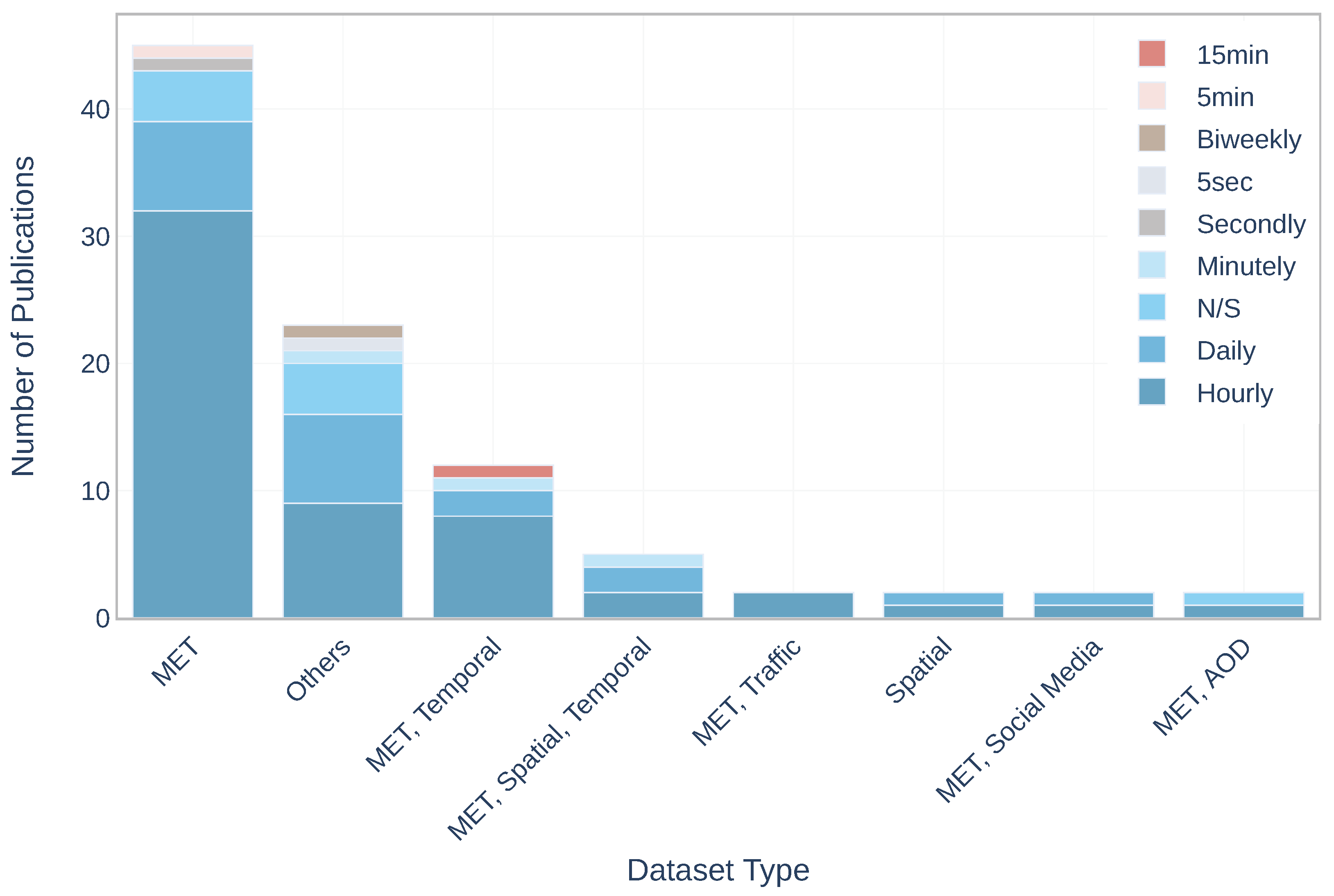
Data Rate: is the timespan during which the sensors provided data. Figure 6 shows the distribution of dataset combinations in terms of data rate. Overall, biweekly, daily, hourly, minutely, secondly, 15 min, 5 min, 5 s data rates were used in the studies, and nine studies did not provide information about data rate. It can be seen, that hourly data rate being the most used (fifty-six papers) is utilised in the publications with all combinations, particularly with ‘MET’ it was the most used combination by researchers (thirty-two papers).
Period (Days): is the period (the number of days) of the data collection. The summary statistics of these days reveals a mean of days of 1300.63 days (Std.Dev: 1484.68) and a median of 731 days (Min: 3 and Max: 8023).
The most used periods are 365 days in nine papers. The result shows that connecting this feature with the data rate, it can give an idea about the volume of the data used for the analysis. Obviously, it cannot provide any guarantee about the quality of data, and it can include noisy data; however, we assume that the final utilised data were not reduced significantly after the data cleaning process.
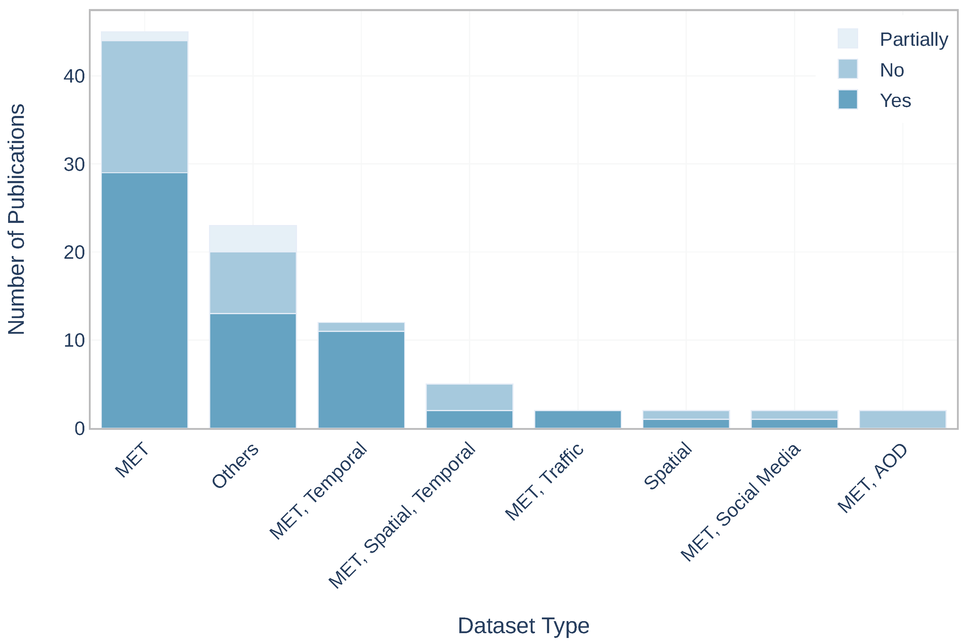
Open Data: contains information about data availability. Figure 7 illustrates the distribution of dataset combinations in terms of data availability. There are three categories: Yes, No, Partially. The first two, basically, show if the authors provide or do not provide data used in the studies, the papers with Partially refer to the studies where the authors provided only the part of data. It is interesting to know about data accessibility throughout the period. From Figure 8 it is detectable that since 2012 the authors had started to use open data in their research, which, interestingly, corresponds to the period when the idea of open data portals [18,19] and smart cities [20] has appeared. Figure 9 displays the data availability per case study. It can be observed that China includes all three categories.
It would be also interesting to observe the relation between the authors’ affiliation and the case study of certain research. The results show that in the majority of the papers (55), the affiliations of all the co-authors are located in the corresponding case studies. In eleven papers the author’s affiliations are located in the countries different from case studies. For example, in the following paper [21], the author’s affiliations are located in China and the case study is USA. In twenty-seven papers, the co-authors’ affiliation partially correspond to the case study. For instance, in this paper [22] the case study is Canada and the author’s affiliations belong to China and Canada.
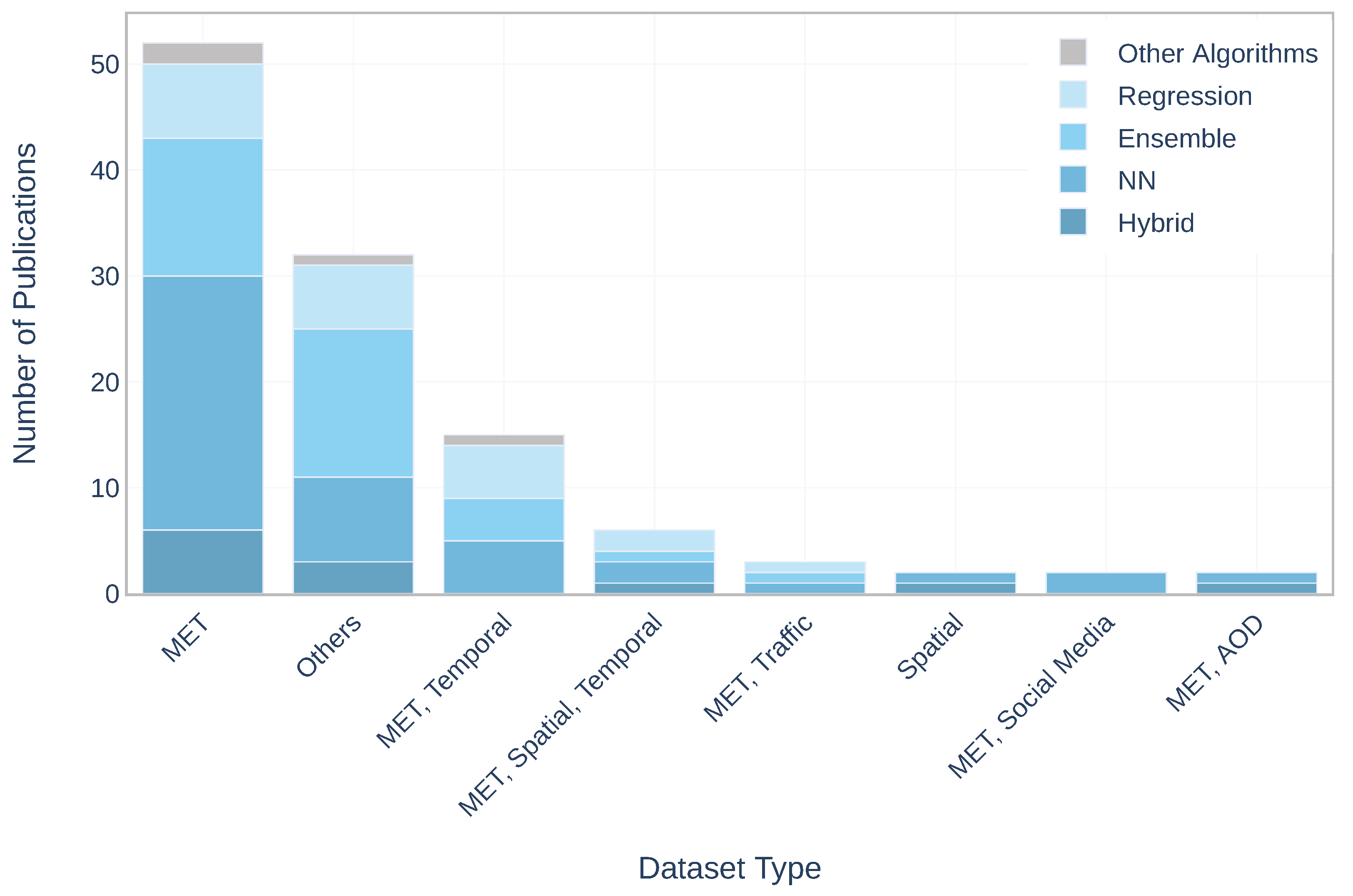
Algorithm: are the ML algorithms on which the applied methods are based. Figure 10 shows the distribution of dataset combinations in terms of ML algorithms. The ML algorithms used in the studies are Neural Network (NN), Regression, Ensemble, Hybrid Model and Other Algorithms. Here are the main methods used in each category: NN—Long Short Term Memory (LSTM), Multilayer Perceptron (MLP), Gated recurrent unit (GRU); Regression—Support Vector Machine (SVM); Ensemble—Random Forest (RF), Extreme Gradient Boosting (XGBoost), Light Gradient Boosted Machine (LightGBM); Hybrid Model—the majority of the methods of this category are based on SVM, for example Partial Least Square-SVM, Multi-output SVM and Multi-Task Learning (MM-SVM); Other Algorithms—includes the works applied Decision Tree Algorithm (C4.8), Reinforcement Learning, Bayesian Model, Regularization and Optimization. It should be pointed out, that in contrast other dataset combinations, ‘MET’ and ‘Others’ include all categories of the algorithms.
Having different prediction targets and methods, it would be valuable to see if there is any relation between targets and applied methods in order to figure out which methods are used to predict a particular target. According to the results of the study, the following connection was detected (main prediction targets and corresponding methods): PM- LSTM, SVM, RF; O3- MLP, RNN; NOx-SVM, RF, RNN; SO2-SVM; CO-LSTM; AQI-SVM.
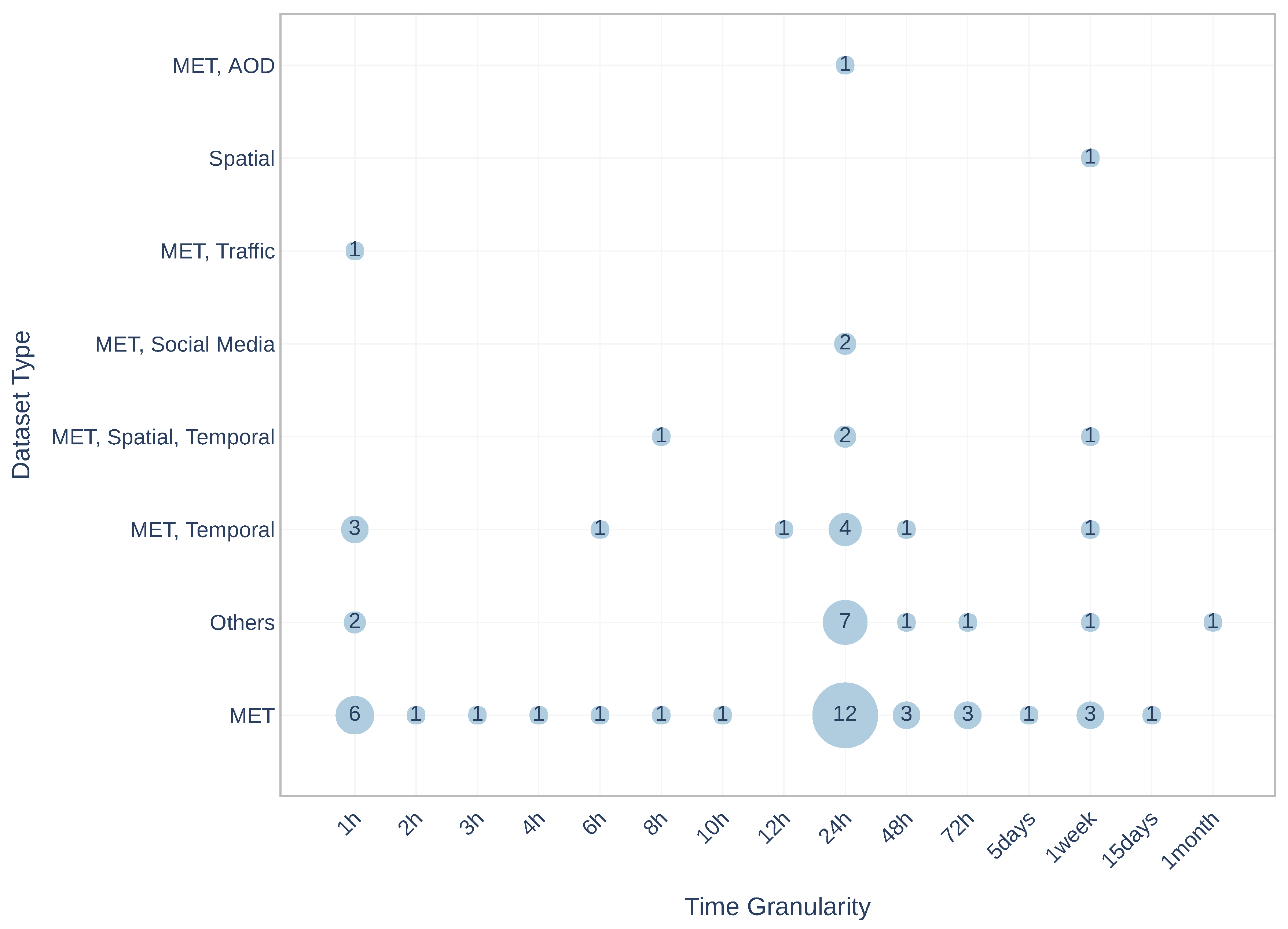
Time Granularity: is the time interval, for which period the prediction was applied. Figure 11 shows the distribution of dataset combinations in terms of time resolution. The used time resolutions are 1 h, 2 h, 3 h, 4 h, 6 h, 8 h, 10 h, 12 h, 24 h, 48 h, 72 h, five days, one week, 15 days and one month. It must be mentioned that these extracted intervals are the maximum intervals applied in each article. It is detectable that 24 h is the most used time resolution regarding the number of publications and different dataset combinations. Furthermore, it can be seen, that the most extended prediction time resolution, one month, is applied in publication with ‘Others’ combination, and considering that the longer resolution decreases the accuracy, it can be seen that there is only one paper implemented prediction for one month.
Evaluation Metric: are the measures which were used to evaluate the applied method. Overall, sixty-nine metrics were used to evaluate the methods, from which the most used metrics are Root Mean Square Error (RMSE) in seventy-seven papers, Mean Absolute Error (MAE) in forty-two papers. Figure 12 demonstrates the distribution of dataset combinations in terms of evaluation metric (each database combination is marked with a different color). It can be shown, that compared to other dataset types ‘MET’, ‘MET, Temporal’ and ‘Others’ were combined with more metrics, particularly, RMSE with ‘MET’ (forty-one papers) and MAE with ‘MET’ (twenty-four papers) are the most used combinations. Additionally, taking into consideration the most used prediction target (PM2.5) and the most used time resolution (24 h), the results show that PM2.5 was a prediction target in eighteen papers with the combination of RMSE and ‘MET’, and in ten papers with the combination of MAE with ‘MET’, and 24 h was a predicted time resolution in ten papers with RMSE and ‘MET’ combination and in six papers with MAE and ‘MET’ combination. Furthermore, the metrics that have been used in more than six publications with corresponding equations and descriptions are extracted and displayed in Table 3. The metrics are RMSE, MAE, Coefficient of Determination (R2), Correlation Coefficient (R), Mean Absolute Percentage Error (MAPE), Index of Agreement (IA), Mean Square Error (MSE), Normalised Root Mean Square Error (NRMSE) [23,24,25,26,27,28,29,30].
Another point to which attention should be paid is understanding in the world of evaluation metrics how to choose the best and the most acceptable model. To select the best model, the majority of the authors selected different benchmark models and, applying the same validation metrics to all models, chose the outperformed model. Only a few authors, such as Goulier et al. [31] and Zhang et al. [32] have focused on the importance to test whether the model performs well enough, acceptable or not. It is important to follow up on evaluation studies to ensure that the evaluation procedure is correct. For example, the articles by Kadiyala and Kumar [33], Alexander et al. [34], Janssen et al. [35] can serve as a guide for researchers.
It is worth mentioning the limitations noted by the authors in their works. The accuracy of model performance depends on many factors, such as ML algorithms, spatial characteristics, prediction targets, temporal resolution, etc. Several authors have mentioned the structural limitations of algorithms, such as the tendency to overfit, complexity, difficulty with interpretation, and time-consuming [36,37,38]. Regarding the prediction target, depending on which pollutant is the prediction target the accuracy may vary since the chemical structure of the pollutants is different. For example, Li et al. in their study [39] found out that the proposed model predicts better PM2.5 than NOx, as NOx is highly reactive and has larger temporal variability. Therefore, many studies mentioned the implementation of the proposed model for predicting other pollutants as future work [21,40]. Another limitation is the lack of data in spatiotemporal resolution [41,42]. Missing values can also be included in this scope, depending on their quantity, the performance can be significantly reduced [43,44]. An important factor is the presence of sudden changes. One solution might be to collect more data, as the training dataset will include more sudden changes, which in turn will lead to better performance in case of sudden changes [42]. Including other datasets such as aerosol optical depth data and meteorological data can help to overcome this issue [45]. It might also be useful to apply techniques for handling imbalanced datasets [40]. Another limitation that we have already mentioned is a prediction with the long temporal resolution since due to the accumulated error, the accuracy decreases as the temporal resolution increases [46,47].
4. Conclusions
Predicting air quality with higher accuracy is gaining in importance and necessity day by day. Therefore, it is very essential to explore the state-of-the-art of the field. Of the numerous aspects that exist in the field of research, this article, through reviewing studies, focuses on datasets in order to examine which datasets are used by researchers and to identify additional variables that they have taken into account in their analysis to predict air quality. A set of the most relevant papers in this field have been selected using ACM, IEEE Xplore, Scopus and WoS databases. Overall, ninety-three papers were selected, reviewed and, afterwards, the essential dataset features were extracted and synthesised (Year, Case Study, Prediction Target, Dataset Type, Data Rate, Period (Days), Open Data, Algorithm and Time Granularity). The results show that twenty-six datasets are used to supplement data collected by air quality sensors, including ‘MET’, ‘Temporal’, ‘Spatial’ and ‘Social Media’, among others. The results show a significant difference on the use of ‘MET’, which is the dominant dataset used in 94.6% of the studies, and 48.4% of the studies combined with only air quality data.
Regarding data availability, it was shown that since 2012 a new stage has begun, associated with the use of open data portals [48], which is crucial for science and contributes to the improvement and development of various research fields and encourages the emergence of new exciting results, which, in turn, has also led to an increase in the number of publications.
A very important finding is to explore and understand which methods are most commonly used and dominant in the field to predict a specific target, for example, to predict particulate matter, LSTM, SVM and RF were found to be the most commonly used methods.
In general, it may be inferred that extra datasets can have significant importance, and involving them in the analysis could improve air quality prediction and obtain more accurate results. However, it is difficult to indicate which datasets are more valuable and it should also be noted that it is not always advisable to include many datasets, as having a huge dataset can be a problem as it requires more training time and may contain redundant data.
Therefore, future work can be addressed to the establishment of a framework based on the same conditions (model, prediction target, evaluation metric, time resolution) with the objective to validate and compare the improvement of each dataset type.
Author Contributions
Conceptualisation, D.I. and F.R.; Formal analysis, S.T.; Funding acquisition, S.T.; Methodology, D.I. and F.R.; Supervision, S.T. and F.R.; Writing—original draft, D.I.; Writing—review & editing, S.T. and F.R. All authors have read and agreed to the published version of the manuscript.
Funding
Ditsuhi Iskandaryan has been funded by the predoctoral programme PINV2018—Universitat Jaume I (PREDOC/2018/61). S.T. has been funded by the Juan de la Cierva—Incorporación postdoctoral programme of the Ministry of Science and Innovation—Spanish government (IJC2018-035017-I). This work has been funded by the Generalitat Valenciana through the Subvenciones para la realización de proyectos de I+D+i desarrollados por grupos de investigación emergentes program (GV/2020/035).
Institutional Review Board Statement
Not applicable.
Informed Consent Statement
Not applicable.
Data Availability Statement
The data presented in this study are openly available in Zenodo at https://doi.org/10.5281/zenodo.4302469 (accessed on 3 January 2021).
Conflicts of Interest
The authors declare no conflict of interest. The funders had no role in the design of the study; in the collection, analyses, or interpretation of data; in the writing of the manuscript, or in the decision to publish the results.
Appendix A

Table A1.
Features of the selected papers. : Not Specified. Published in Zenodo with this following doi: https://doi.org/10.5281/zenodo.4302469 [49]. (accessed on 27 February 2021).
Table A1.
Features of the selected papers. : Not Specified. Published in Zenodo with this following doi: https://doi.org/10.5281/zenodo.4302469 [49]. (accessed on 27 February 2021).
| Work | Year | Case Study | Prediction Target | Dataset Type | Data Rate | Period (Days) | Open Data | Algorithm | Time Granularity | Evaluation Metric |
|---|---|---|---|---|---|---|---|---|---|---|
| [36] | 2020 | USA | PM2.5 | Spatial, Temporal, AOD, PBL Height | Daily | 5779 | No | Hybrid | 24 h | RMSE, SD, R2 |
| [50] | 2020 | Canada | UFP | MET, Traffic, Land Use, BEV | N/S | 120 | No | Ensemble | RMSE, R2 | |
| [51] | 2020 | Taiwan | PM2.5, PM10 | MET | N/S | 2192 | No | Hybrid | 8 h | RMSE, MAE |
| [39] | 2020 | China | PM2.5, NOx | MET, Traffic | Hourly | 731 | No | Regression, Ensemble | 1 h | RMSE, ME, NRMSE, NME, POD, POF, R2 |
| [21] | 2020 | USA | PM2.5 | MET, Temporal | Hourly | 730 | No | NN | RMSE, MAE, MAPE | |
| [42] | 2020 | India | PM2.5 | MET | Hourly | 1230 | No | NN | RMSE, R2 | |
| [52] | 2020 | USA | AQI | MET | Hourly | 851 | Yes | Regression | 1 h | RMSE, MAE, NRMSE, R |
| [53] | 2020 | Turkey | PM10 | Spatial, Land Use | N/S | 3652 | No | Regression, Ensemble, NN | RMSE, MAE, R2 | |
| [54] | 2020 | China | PM2.5 | MET | Hourly | 31 | Yes | NN | 1 h | RMSE, R |
| [55] | 2020 | China | AQHI, IAQL | MET, Temporal | Hourly | 730/1826 | Yes | Ensemble | 12 h | Acc, MSE, WP, WR, WF |
| [56] | 2020 | China | PM10 | MET | Daily | 1096 | No | NN | 24 h | RMSE, ME, R, EOp |
| [37] | 2020 | Tunisia, Italy | MET, Temporal | Hourly | 1461/366 | No | Ensemble | 1 week | aRRMSE, aRMSE, R2, aCC, MSE, aRE, RP | |
| [38] | 2020 | China | PM2.5 | MET | N/S | 46 | Yes | Ensemble | 24 h | RMSE, MAE, SMAPE |
| [41] | 2020 | China | PM2.5 | MET | Hourly | 1825 | No | NN | 1 week | RMSE |
| [57] | 2020 | China | PM2.5 | MET | N/S | 1096 | Yes | NN | 24 h | RMSE, MAE, MAPE |
| [46] | 2020 | China | O3 | MET, UV Index | Daily | 1491 | Yes | Hybrid | 1 week | RMSE, MAE, MAPE, IA |
| [58] | 2020 | South Korea | PM2.5, PM10 | MET | Hourly | 1461 | Yes | Hybrid | 15days | RMSE, MAE |
| [40] | 2020 | China | PM2.5, PM10, NO2, NO, CO | MET | Daily | 4656 | No | NN | 24 h | MSE |
| [59] | 2020 | Taiwan | PM2.5 | MET, Spatial, Temporal | Hourly | 365 | Yes | Ensemble | 24 h | RMSE, NRMSE, R2 |
| [60] | 2020 | UK | PM2.5 | MET, Spatial, Temporal, AOD, Land Use | Daily | 3287 | Partially | Ensemble | 24 h | RMSE, MSE, R2 |
| [61] | 2020 | Ecuador | PM2.5 | MET, Spatial, Temporal, Traffic | 5 s | 4 | No | Other Algorithms | Acc | |
| [62] | 2020 | China | PM2.5 | MET | Hourly | 365 | No | Ensemble | 48 h | MSE, IA, NMGE, R2 |
| [63] | 2020 | China | PM2.5 | MET | Hourly | 1461 | No | Ensemble | 24 h | RMSE, MB, ME, R |
| [64] | 2020 | China | AQI | MET | Hourly | 2192 | No | NN | 48 h | RMSE, Acc |
| [32] | 2020 | China | AQI | MET | Hourly | 730 | Yes | NN | 24 h | RMSE, MAE, R2, FB |
| [65] | 2020 | South Korea | PM2.5, PM10 | MET, Temporal, Spatial | Minutely | 7 | No | Hybrid | RMSE | |
| [66] | 2020 | China | PM2.5, PM10, O3, NO2, SO2, CO | MET, Social Media | Daily | 731 | Yes | NN | 24 h | RMSE, MAE |
| [67] | 2020 | Thailand | PM10 | MET | Secondly | 59 | No | NN | 1 h | RMSE, MAE, MAPE, R |
| [68] | 2020 | China | AQI | Spatial | Daily | 1086 | Yes | Hybrid | 5 days | RMSE, MAE, MAPE, R |
| [31] | 2020 | Germany | CO2, NH3, NO, NO2, NOx, O3, PM1, PM2.5, PM10, PN10 | MET, Temporal, Traffic, SP | Hourly | 62 | No | NN | 1 h | RMSE, R, NMB, NMSD, RS, SD, SD |
| [43] | 2020 | Mongolia | PM2.5 | MET, Temporal, Land Use, PD | Hourly | 2922 | No | Regression, Ensemble | 24 h | RMSE, R2 |
| [44] | 2020 | Taiwan | PM2.5 | MET, Temporal, Spatial | Hourly | 2192 | No | NN | 8 h | RMSE, MAE, MAPE |
| [69] | 2020 | Turkey | PM10 | MET | Daily | 766 | No | Regression, NN | RMSE, MAE, R2 | |
| [70] | 2020 | Jordan | O3 | MET, Temporal | Daily | 1496 | No | NN, Regression, Ensemble | 24 h | RMSE, MAE, R2 |
| [71] | 2019 | South Korea | PM10, PM2.5 | MET, Spatial, Human Movements | Hourly | 115 | No | NN, Regression | 1 h | RMSE, R2 |
| [72] | 2019 | China/Taiwan | PM2.5 | MET | Hourly | 3693 | No | NN, Other Algorithms | 5 days | RMSE |
| [73] | 2019 | South Korea | O3 | MET | Hourly | 1096 | No | Ensemble | 24 h | IA |
| [74] | 2019 | USA | NO2, NOx | MET, Spatial, Traffic | biweekly | 8023 | No | Ensemble | RMSE, R2, RMSEIQR | |
| [6] | 2019 | Europe | NO2, PM2.5 | AOD, Traffic, Land Use, Altitude | N/S | 365 | Yes | Regression, Ensemble, NN | RMSE, R2, MSE-R2 | |
| [75] | 2019 | China | PM2.5 | MET, AOD | Hourly | 1096 | Yes | Hybrid | 24 h | RMSE, R2 |
| [76] | 2019 | China | SO2 | MET, Temporal, Land Use, OMI-SO2, PPS, TS | Daily | 365 | Partially | Hybrid | 24 h | RMSE, R2, RPE |
| [77] | 2019 | China | PM2.5 | MET | Hourly | 731 | No | NN | 3 h | RMSE |
| [78] | 2019 | China | PM2.5 | MET, WFD, Spatial | N/S | 61 | No | Ensemble | 24 h | MAE, SMAPE, MSE |
| [79] | 2019 | China | PM2.5 | MET | Hourly | 1826 | Yes | NN | 2 h | RMSE, MAE, SMAPE |
| [80] | 2019 | China | PM2.5 | MET | N/S | 2191 | Yes | Ensemble | 1 week | RMSE, MAE |
| [81] | 2019 | Italy | CO(GT), NO2(GT) | MET | Hourly | 183 | Yes | NN | 1 h | RMSE, MAE, MAPE |
| [82] | 2019 | China | PM2.5 | Spatial | Hourly | 365 | No | NN | 1 week | RMSE, MAE, MAPE |
| [7] | 2019 | China | AQI | MET, WFD, Traffic, POI Distribution, FAPE, RND | Hourly | 366 | Yes | NN | 48 h | MAE, MAP |
| [83] | 2019 | Taiwan | PM2.5 | MET | Hourly | 2557 | No | Hybrid | 4 h | RMSE, Gbench |
| [84] | 2019 | Iran | PM2.5 | MET | Hourly | 1826 | No | Ensemble, NN, Hybrid | 48 h | RMSE, MAE, R2 |
| [85] | 2019 | Poland | NO2 | MET, Temporal, Traffic | Hourly | 731 | No | Ensemble | MAPE, MADE, BIC, R2 | |
| [86] | 2019 | India | O3, PM2.5, NOx, CO | MET, Traffic | Hourly | 730 | No | NN | RMSE, NSE, PBIAS, R | |
| [87] | 2019 | China | PM2.5 | MET | Hourly | 1826 | No | NN | 72 h | RMSE, IA, MAE, R |
| [47] | 2019 | China | PM2.5 | MET | Hourly | 366 | No | NN | 10 h | RMSE, NRMSE, MAE, SMAPE, R |
| [88] | 2019 | China | PM2.5 | MET, AOD | N/S | 730 | Yes | NN | RMSE, MAE, MSE, R2 | |
| [89] | 2019 | Iran | PM2.5 | MET, Temporal, Spatial, AOD, Altitude | Daily | 1460 | Yes | Ensemble, NN | RMSE, MAE, R2 | |
| [90] | 2019 | India | O3 | MET | Hourly | 92 | No | Ensemble | IoAd, R2, PEP | |
| [91] | 2019 | China | O3 | MET | Hourly | 365 | No | Ensemble, NN | RMSE, R, NMB, NME, MFB, MFE | |
| [92] | 2019 | UK | SO2 | MET | Hourly | 120 | Yes | Ensemble | RMSE, MAE, R2, RAE | |
| [93] | 2019 | Taiwan | AQI | MET, Temporal | Hourly | 851 | No | Regression, NN | 6 h | RMSE, MAE, R2 |
| [94] | 2019 | Iran | PM10, PM2.5 | MET, Temporal, Spatial | Daily | 3652 | Yes | Regression, NN | 1 week | RMSE, R2 |
| [95] | 2018 | China | PM2.5 | MET, Temporal, AOD | Hourly | 731 | Partially | NN | 72 h | RMSE, MAE, MSE, IA, TPR, FPR, SI |
| [96] | 2018 | Slovenia | PM10, O3 | MET, Temporal | Hourly | 1461 | No | Other Algorithms | 24 h | MAE, RPS |
| [8] | 2018 | China | O3 | MET, Land Use, Elevation, AEI, NDVI, RND, PD | Hourly | 365 | Yes | Ensemble | RMSE, R2, RPE | |
| [9] | 2018 | China | PM2.5 | MET, AOD, Elevation, PD, RND, NDVI | Daily | 1095 | Yes | Ensemble | 1 month | RMSE, R2, RPE |
| [97] | 2018 | China | PM2.5 | MET, Spatial | Hourly | 61 | No | Regression | 24 h | total accuracy index (pt), a total absolute error index (et) |
| [98] | 2018 | UK | AQI | MET | Hourly | 605 | Yes | NN | RMSE, MAPE, band Acc | |
| [99] | 2018 | Kuwait | O3 | MET | Hourly | 669 | No | NN | 72 h | RMSE, MAE |
| [100] | 2018 | Spain | O3 | MET | Hourly | 730 | Yes | Ensemble | 24 h | RMSE, MAE, R2 |
| [101] | 2018 | Egypt | PM10 | MET, Temporal | Hourly | 276 | No | Regression | 1 h | RMSE, R, t-Value |
| [102] | 2018 | China | PM2.5 | MET | Hourly | 1826 | No | NN | 1 h | RMSE, MAE, IA, R |
| [103] | 2018 | USA | O3, PM2.5, SO2 | MET | Hourly | 3652 | Yes | Other Algorithms | 24 h | RMSE |
| [104] | 2017 | USA | BC | MET, Spatial, Temporal | Daily | 4383 | Yes | Regression | 24 h | R2 |
| [22] | 2017 | Canada | O3, PM2.5, NO2 | MET, Temporal | Hourly | 1826 | No | NN | 48 h | MAE, R, ME, SS |
| [105] | 2017 | China | PM2.5 | MET, Social Media | Hourly | 365 | No | NN | 24 h | RMSE |
| [106] | 2017 | Ecuador | PM2.5 | MET | Daily | 1827 | No | Ensemble, Regression, NN | MSE, MAPE | |
| [107] | 2017 | China | PM2.5 | MET, Temporal, Spatial, AOD | Daily | 365 | Yes | Ensemble | RMSE, R2 | |
| [108] | 2017 | Kuwait | PNCs | MET | 5min | 30 | No | NN | RMSE, NRMSE, IA, R2 | |
| [109] | 2017 | Egypt | PM10 | MET, Temporal | Hourly | 368 | No | Regression | 1 h | RMSE, R, z’, t-value |
| [110] | 2017 | China | NO2, NOx, O3, PM2.5, SO2 | MET, Temporal | Daily | 2191 | No | NN | 24 h | RMSE, MAE, IA, R2 |
| [111] | 2017 | China | AQI | MET | Daily | 851 | No | Regression | RMSE, MAE, MAPE, MSE | |
| [112] | 2016 | Qatar | O3, NO2, SO2 | MET, Temporal | 15min | 92 | No | Regression | 24 h | RMSE, NRMSE, PTA |
| [113] | 2016 | France | O3, NO2, PM10 | MET | Hourly | 1733 | No | Hybrid | 24 h | RMSE, MAE, NRMSE, MBE, IA, R |
| [114] | 2014 | Saudi Arabia | PM10 | MET | Hourly | 366 | No | Regression | 1 h | RMSE, MAE, MBE, FACT2, R, IA |
| [115] | 2014 | France | O3, NO2, PM10 | MET | Hourly | 731 | Yes | Ensemble | 72 h | RMSE |
| [16] | 2013 | China | PM1.0, UFP | MET, Traffic, Temporal | Minutely | 3 | No | Regression, Ensemble, NN | AUC, R, R2, Precision, Recall, f measure, weighted f-measure | |
| [116] | 2013 | Greece | O3 | MET | Hourly | 7305 | No | NN | 6 h | RMSE, R2, R |
| [117] | 2013 | India | AQI | MET | Daily | 1825 | Partially | Ensemble | RMSE, MAE, R | |
| [118] | 2012 | China | SPM, SO2, NO2, O3 | MET | Daily | 1095 | Yes | Regression | 24 h | RMSE, MAE, CWIA, RE |
| [119] | 2012 | Iran | CO | MET | Hourly | 1492 | No | Hybrid | 24 h | RMSE, RME, MARE, R2 |
| [120] | 2012 | Saudi Arabia | O3 | MET, Temporal | Minutely | 183 | No | NN, Ensemble | 1 h | MAE, MAPE, SD, MD, R |
| [121] | 2009 | Europe | O3 | MET, Land Data, Chemical, Emission | Hourly | 120 | No | Ensemble | 24 h | RMSE |
| [122] | 2008 | China | RSP(PM10), NOx, SO2 | MET | Hourly | 61 | No | Regression | 1 week | RMSE, MAE, WIA |
References
- World Urbanization Prospects. Available online: https://www.un.org/development/desa/publications/2018-revision-of-world-urbanization-prospects.html (accessed on 5 March 2020).
- Air Pollution. Available online: https://www.who.int/health-topics/air-pollution#tab=tab_1/ (accessed on 13 March 2020).
- Ambient Air Pollution: Pollutants. Available online: https://www.who.int/airpollution/ambient/pollutants/en/ (accessed on 28 November 2020).
- Air Quality Assessment and Forecast System: Near-Term Opportunity Plan. Available online: https://www.earthobservations.org/documents/committees/uic/200704_4thUIC/Air_Quality_NTO_2006-0925.pdf (accessed on 27 April 2020).
- Ramos, F.; Trilles, S.; Muñoz, A.; Huerta, J. Promoting pollution-free routes in smart cities using air quality sensor networks. Sensors 2018, 18, 2507. [Google Scholar] [CrossRef] [Green Version]
- Chen, J.; de Hoogh, K.; Gulliver, J.; Hoffmann, B.; Hertel, O.; Ketzel, M.; Bauwelinck, M.; van Donkelaar, A.; Hvidtfeldt, U.A.; Katsouyanni, K.; et al. A comparison of linear regression, regularization, and machine learning algorithms to develop Europe-wide spatial models of fine particles and nitrogen dioxide. Environ. Int. 2019, 130, 104934. [Google Scholar] [CrossRef] [PubMed]
- Chen, L.; Ding, Y.; Lyu, D.; Liu, X.; Long, H. Deep multi-task learning based urban air quality index modelling. Proc. ACM Interact. Mob. Wearable Ubiquitous Technol. 2019, 3, 1–17. [Google Scholar] [CrossRef]
- Zhan, Y.; Luo, Y.; Deng, X.; Grieneisen, M.L.; Zhang, M.; Di, B. Spatiotemporal prediction of daily ambient ozone levels across China using random forest for human exposure assessment. Environ. Pollut. 2018, 233, 464–473. [Google Scholar] [CrossRef] [PubMed]
- Huang, K.; Xiao, Q.; Meng, X.; Geng, G.; Wang, Y.; Lyapustin, A.; Gu, D.; Liu, Y. Predicting monthly high-resolution PM2.5 concentrations with random forest model in the North China Plain. Environ. Pollut. 2018, 242, 675–683. [Google Scholar] [CrossRef] [PubMed]
- Degbelo, A.; Granell, C.; Trilles, S.; Bhattacharya, D.; Wissing, J. Tell me how my open Data are re-used: Increasing transparency through the Open City Toolkit. In Open Cities | Open Data; Springer: Singapore, 2020; pp. 311–330. [Google Scholar]
- Benitez-Paez, F.; Comber, A.; Trilles, S.; Huerta, J. Creating a conceptual framework to improve the re-usability of open geographic data in cities. Trans. GIS 2018, 22, 806–822. [Google Scholar] [CrossRef] [Green Version]
- Liberati, A.; Altman, D.G.; Tetzlaff, J.; Mulrow, C.; Gøtzsche, P.C.; Ioannidis, J.P.; Clarke, M.; Devereaux, P.J.; Kleijnen, J.; Moher, D. The PRISMA statement for reporting systematic reviews and meta-analyses of studies that evaluate health care interventions: Explanation and elaboration. J. Clin. Epidemiol. 2009, 62, e1–e34. [Google Scholar] [CrossRef] [Green Version]
- Degbelo, A.; Granell, C.; Trilles, S.; Bhattacharya, D.; Casteleyn, S.; Kray, C. Opening up smart cities: Citizen-centric challenges and opportunities from GIScience. ISPRS Int. J. Geo-Inf. 2016, 5, 16. [Google Scholar] [CrossRef] [Green Version]
- Particle Numbers and Concentrations Network. Available online: https://uk-air.defra.gov.uk/networks/network-info?view=particle#:~:text=Particle%20number%20concentration%20is%20the,typically%20dominated%20by%20larger%20particles (accessed on 21 January 2021).
- Vallero, D.A. Fundamentals of Air Pollution; Academic Press: Cambridge, MA, USA, 2014. [Google Scholar]
- Pandey, G.; Zhang, B.; Jian, L. Predicting submicron air pollution indicators: A machine learning approach. Environ. Sci. Process. Impacts 2013, 15, 996–1005. [Google Scholar] [CrossRef]
- Giechaskiel, B.; Lähde, T.; Gandi, S.; Keller, S.; Kreutziger, P.; Mamakos, A. Assessment of 10-nm Particle Number (PN) Portable Emissions Measurement Systems (PEMS) for Future Regulations. Int. J. Environ. Res. Public Health 2020, 17, 3878. [Google Scholar] [CrossRef]
- Attard, J.; Orlandi, F.; Scerri, S.; Auer, S. A systematic review of open government data initiatives. Gov. Inf. Q. 2015, 32, 399–418. [Google Scholar] [CrossRef]
- Máchová, R.; Lnenicka, M. Evaluating the quality of open data portals on the national level. J. Theor. Appl. Electron. Commer. Res. 2017, 12, 21–41. [Google Scholar] [CrossRef] [Green Version]
- Albino, V.; Berardi, U.; Dangelico, R.M. Smart cities: Definitions, dimensions, performance, and initiatives. J. Urban Technol. 2015, 22, 3–21. [Google Scholar] [CrossRef]
- Ma, J.; Ding, Y.; Cheng, J.C.; Jiang, F.; Gan, V.J.; Xu, Z. A Lag-FLSTM deep learning network based on Bayesian Optimization for multi-sequential-variant PM2.5 prediction. Sustain. Cities Soc. 2020, 60, 102237. [Google Scholar] [CrossRef]
- Peng, H.; Lima, A.R.; Teakles, A.; Jin, J.; Cannon, A.J.; Hsieh, W.W. Evaluating hourly air quality forecasting in Canada with nonlinear updatable machine learning methods. Air Qual. Atmos. Health 2017, 10, 195–211. [Google Scholar] [CrossRef]
- Botchkarev, A. Performance metrics (error measures) in machine learning regression, forecasting and prognostics: Properties and typology. arXiv 2018, arXiv:1809.03006. [Google Scholar]
- Hossin, M.; Sulaiman, M. A review on evaluation metrics for data classification evaluations. Int. J. Data Min. Knowl. Manag. 2015, 5, 1. [Google Scholar]
- Ivy, D.; Mulholland, J.A.; Russell, A.G. Development of ambient air quality population-weighted metrics for use in time-series health studies. J. Air Waste Manag. Assoc. 2008, 58, 711–720. [Google Scholar] [CrossRef] [Green Version]
- Tian, Y.; Nearing, G.S.; Peters-Lidard, C.D.; Harrison, K.W.; Tang, L. Performance metrics, error modeling, and uncertainty quantification. Mon. Weather Rev. 2016, 144, 607–613. [Google Scholar] [CrossRef]
- Kim, S.; Kim, H. A new metric of absolute percentage error for intermittent demand forecasts. Int. J. Forecast. 2016, 32, 669–679. [Google Scholar] [CrossRef]
- Yu, S.; Eder, B.; Dennis, R.; Chu, S.H.; Schwartz, S.E. New unbiased symmetric metrics for evaluation of air quality models. Atmos. Sci. Lett. 2006, 7, 26–34. [Google Scholar] [CrossRef]
- Willmott, C.J.; Wicks, D.E. An empirical method for the spatial interpolation of monthly precipitation within California. Phys. Geogr. 1980, 1, 59–73. [Google Scholar] [CrossRef]
- Nagelkerke, N.J.D. A note on a general definition of the coefficient of determination. Biometrika 1991, 78, 691–692. [Google Scholar] [CrossRef]
- Goulier, L.; Paas, B.; Ehrnsperger, L.; Klemm, O. Modelling of urban air pollutant concentrations with artificial neural networks using novel input variables. Int. J. Environ. Res. Public Health 2020, 17, 2025. [Google Scholar] [CrossRef] [Green Version]
- Zhang, K.; Thé, J.; Xie, G.; Yu, H. Multi-step ahead forecasting of regional air quality using spatial-temporal deep neural networks: A case study of Huaihai Economic Zone. J. Clean. Prod. 2020, 277, 123231. [Google Scholar] [CrossRef]
- Kadiyala, A.; Kumar, A. Evaluation of indoor air quality models with the ranked statistical performance measures using available software. Environ. Prog. Sustain. Energy 2012, 31, 170–175. [Google Scholar] [CrossRef]
- Alexander, D.L.; Tropsha, A.; Winkler, D.A. Beware of R2: Simple, unambiguous assessment of the prediction accuracy of QSAR and QSPR models. J. Chem. Inf. Model. 2015, 55, 1316–1322. [Google Scholar] [CrossRef] [Green Version]
- Guidance Document on Modelling Quality Objectives and Benchmarking. Available online: https://fairmode.jrc.ec.europa.eu/document/fairmode/WG1/Guidance_MQO_Bench_vs3.1.1.pdf (accessed on 20 February 2021).
- Just, A.C.; Arfer, K.B.; Rush, J.; Dorman, M.; Shtein, A.; Lyapustin, A.; Kloog, I. Advancing methodologies for applying machine learning and evaluating spatiotemporal models of fine particulate matter (PM2.5) using satellite data over large regions. Atmos. Environ. 2020, 239, 117649. [Google Scholar] [CrossRef]
- Masmoudi, S.; Elghazel, H.; Taieb, D.; Yazar, O.; Kallel, A. A machine-learning framework for predicting multiple air pollutants’ concentrations via multi-target regression and feature selection. Sci. Total Environ. 2020, 715, 136991. [Google Scholar] [CrossRef]
- Zhang, Y.; Zhang, R.; Ma, Q.; Wang, Y.; Wang, Q.; Huang, Z.; Huang, L. A feature selection and multi-model fusion-based approach of predicting air quality. ISA Trans. 2020, 100, 210–220. [Google Scholar] [CrossRef] [PubMed]
- Li, Z.; Yim, S.H.L.; Ho, K.F. High temporal resolution prediction of street-level PM2.5 and NOx concentrations using machine learning approach. J. Clean. Prod. 2020, 268, 121975. [Google Scholar] [CrossRef]
- Fong, I.H.; Li, T.; Fong, S.; Wong, R.K.; Tallón-Ballesteros, A.J. Predicting concentration levels of air pollutants by transfer learning and recurrent neural network. Knowl.-Based Syst. 2020, 192, 105622. [Google Scholar] [CrossRef]
- Zhang, B.; Zhang, H.; Zhao, G.; Lian, J. Constructing a PM2.5 concentration prediction model by combining auto-encoder with Bi-LSTM neural networks. Environ. Model. Softw. 2020, 124, 104600. [Google Scholar] [CrossRef]
- Shah, J.; Mishra, B. Analytical Equations based Prediction Approach for PM2.5 using Artificial Neural Network. arXiv 2020, arXiv:2002.11416. [Google Scholar]
- Enebish, T.; Chau, K.; Jadamba, B.; Franklin, M. Predicting ambient PM2.5 concentrations in Ulaanbaatar, Mongolia with machine learning approaches. J. Expo. Sci. Environ. Epidemiol. 2020, 1–10. [Google Scholar] [CrossRef]
- Chang, Y.S.; Chiao, H.T.; Abimannan, S.; Huang, Y.P.; Tsai, Y.T.; Lin, K.M. An LSTM-based aggregated model for air pollution forecasting. Atmos. Pollut. Res. 2020, 11, 1451–1463. [Google Scholar] [CrossRef]
- Wen, C.; Liu, S.; Yao, X.; Peng, L.; Li, X.; Hu, Y.; Chi, T. A novel spatiotemporal convolutional long short-term neural network for air pollution prediction. Sci. Total Environ. 2019, 654, 1091–1099. [Google Scholar] [CrossRef]
- Mo, Y.; Li, Q.; Karimian, H.; Fang, S.; Tang, B.; Chen, G.; Sachdeva, S. A novel framework for daily forecasting of ozone mass concentrations based on cycle reservoir with regular jumps neural networks. Atmos. Environ. 2020, 220, 117072. [Google Scholar] [CrossRef]
- Xu, X.; Ren, W. Prediction of Air Pollution Concentration Based on mRMR and Echo State Network. Appl. Sci. 2019, 9, 1811. [Google Scholar] [CrossRef] [Green Version]
- Benitez-Paez, F.; Degbelo, A.; Trilles, S.; Huerta, J. Roadblocks hindering the reuse of open geodata in Colombia and Spain: A data user’s perspective. ISPRS Int. J. Geo-Inf. 2018, 7, 6. [Google Scholar] [CrossRef] [Green Version]
- Iskandaryan, D.; Ramos, F.; Trilles, S. The Features of the Selected Papers in the Field of Air Quality Prediction. 2020. Available online: http://doi.org/10.5281/zenodo.4302469 (accessed on 27 February 2021).
- Xu, J.; Wang, A.; Schmidt, N.; Adams, M.; Hatzopoulou, M. A gradient boost approach for predicting near-road ultrafine particle concentrations using detailed traffic characterization. Environ. Pollut. 2020, 265, 114777. [Google Scholar] [CrossRef]
- Chang, Y.S.; Abimannan, S.; Chiao, H.T.; Lin, C.Y.; Huang, Y.P. An ensemble learning based hybrid model and framework for air pollution forecasting. Environ. Sci. Pollut. Res. 2020, 27, 38155–38168. [Google Scholar] [CrossRef] [PubMed]
- Castelli, M.; Clemente, F.M.; Popovič, A.; Silva, S.; Vanneschi, L. A Machine Learning Approach to Predict Air Quality in California. Complexity 2020, 2020, 8049504. [Google Scholar] [CrossRef]
- Bozdağ, A.; Dokuz, Y.; Gökçek, Ö.B. Spatial prediction of PM10 concentration using machine learning algorithms in Ankara, Turkey. Environ. Pollut. 2020, 263, 114635. [Google Scholar] [CrossRef]
- Feng, R.; Gao, H.; Luo, K.; Fan, J.R. Analysis and accurate prediction of ambient PM2.5 in China using Multi-layer Perceptron. Atmos. Environ. 2020, 232, 117534. [Google Scholar] [CrossRef]
- Zheng, H.; Cheng, Y.; Li, H. Investigation of model ensemble for fine-grained air quality prediction. China Commun. 2020, 17, 207–223. [Google Scholar] [CrossRef]
- Guo, Q.; He, Z.; Li, S.; Li, X.; Meng, J.; Hou, Z.; Liu, J.; Chen, Y. Air Pollution Forecasting Using Artificial and Wavelet Neural Networks with Meteorological Conditions. Aerosol Air Qual. Res. 2020, 20, 1429–1439. [Google Scholar] [CrossRef]
- Pak, U.; Ma, J.; Ryu, U.; Ryom, K.; Juhyok, U.; Pak, K.; Pak, C. Deep learning-based PM2.5 prediction considering the spatiotemporal correlations: A case study of Beijing, China. Sci. Total Environ. 2020, 699, 133561. [Google Scholar] [CrossRef] [PubMed]
- Yang, G.; Lee, H.; Lee, G. A Hybrid Deep Learning Model to Forecast Particulate Matter Concentration Levels in Seoul, South Korea. Atmosphere 2020, 11, 348. [Google Scholar] [CrossRef] [Green Version]
- Lee, M.; Lin, L.; Chen, C.Y.; Tsao, Y.; Yao, T.H.; Fei, M.H.; Fang, S.H. Forecasting Air Quality in taiwan by Using Machine Learning. Sci. Rep. 2020, 10, 4153. [Google Scholar] [CrossRef] [PubMed]
- Danesh Yazdi, M.; Kuang, Z.; Dimakopoulou, K.; Barratt, B.; Suel, E.; Amini, H.; Lyapustin, A.; Katsouyanni, K.; Schwartz, J. Predicting Fine Particulate Matter (PM2.5) in the Greater London Area: An Ensemble Approach using Machine Learning Methods. Remote Sens. 2020, 12, 914. [Google Scholar] [CrossRef] [Green Version]
- Zalakeviciute, R.; Bastidas, M.; Buenaño, A.; Rybarczyk, Y. A Traffic-Based Method to Predict and Map Urban Air Quality. Appl. Sci. 2020, 10, 2035. [Google Scholar] [CrossRef] [Green Version]
- Gu, K.; Xia, Z.; Qiao, J. Stacked selective ensemble for PM2.5 forecast. IEEE Trans. Instrum. Meas. 2019, 69, 660–671. [Google Scholar] [CrossRef]
- Ma, J.; Yu, Z.; Qu, Y.; Xu, J.; Cao, Y. Application of the xgboost machine learning method in PM2.5 prediction: A case study of shanghai. Aerosol Air Qual. Res. 2020, 20, 128–138. [Google Scholar] [CrossRef] [Green Version]
- Zhang, L.; Li, D.; Guo, Q. Deep Learning From Spatio-Temporal Data Using Orthogonal Regularizaion Residual CNN for Air Prediction. IEEE Access 2020, 8, 66037–66047. [Google Scholar] [CrossRef]
- Zhang, D.; Woo, S.S. Real Time Localized Air Quality Monitoring and Prediction Through Mobile and Fixed IoT Sensing Network. IEEE Access 2020, 8, 89584–89594. [Google Scholar] [CrossRef]
- Zhai, W.; Cheng, C. A long short-term memory approach to predicting air quality based on social media data. Atmos. Environ. 2020, 237, 117411. [Google Scholar] [CrossRef]
- Photphanloet, C.; Lipikorn, R. PM10 concentration forecast using modified depth-first search and supervised learning neural network. Sci. Total Environ. 2020, 727, 138507. [Google Scholar] [CrossRef]
- Liu, H.; Chen, C. Spatial air quality index prediction model based on decomposition, adaptive boosting, and three-stage feature selection: A case study in China. J. Clean. Prod. 2020, 265, 121777. [Google Scholar] [CrossRef]
- Altikat, A. Modeling air pollution levels in volcanic geological regional properties and microclimatic conditions. Int. J. Environ. Sci. Technol. 2020, 17, 2377–2384. [Google Scholar] [CrossRef]
- Hijjawi, M.A.M.S.M. Ground-level Ozone Prediction Using Machine Learning Techniques: A Case Study in Amman, Jordan. Int. J. Autom. Comput. 2020, 17, 667–677. [Google Scholar]
- Kim, S.H.; Son, D.S.; Park, M.H.; Hwang, H.S. Developing a Big Data Analytic Model and a Platform for Particulate Matter Prediction: A Case Study. Int. J. Fuzzy Log. Intell. Syst. 2019, 19, 242–249. [Google Scholar] [CrossRef] [Green Version]
- Chang, S.W.; Chang, C.L.; Li, L.T.; Liao, S.W. Reinforcement Learning for Improving the Accuracy of PM2.5 Pollution Forecast Under the Neural Network Framework. IEEE Access 2019, 8, 9864–9874. [Google Scholar] [CrossRef]
- Eslami, E.; Salman, A.K.; Choi, Y.; Sayeed, A.; Lops, Y. A data ensemble approach for real-time air quality forecasting using extremely randomized trees and deep neural networks. Neural Comput. Appl. 2019, 32, 7563–7579. [Google Scholar] [CrossRef]
- Li, L.; Girguis, M.; Lurmann, F.; Wu, J.; Urman, R.; Rappaport, E.; Ritz, B.; Franklin, M.; Breton, C.; Gilliland, F.; et al. Cluster-based bagging of constrained mixed-effects models for high spatiotemporal resolution nitrogen oxides prediction over large regions. Environ. Int. 2019, 128, 310–323. [Google Scholar] [CrossRef] [PubMed]
- Li, X.; Zhang, X. Predicting ground-level PM2.5 concentrations in the Beijing-Tianjin-Hebei region: A hybrid remote sensing and machine learning approach. Environ. Pollut. 2019, 249, 735–749. [Google Scholar] [CrossRef] [PubMed] [Green Version]
- Li, R.; Cui, L.; Meng, Y.; Zhao, Y.; Fu, H. Satellite-based prediction of daily SO2 exposure across China using a high-quality random forest-spatiotemporal Kriging (RF-STK) model for health risk assessment. Atmos. Environ. 2019, 208, 10–19. [Google Scholar] [CrossRef]
- Qin, D.; Yu, J.; Zou, G.; Yong, R.; Zhao, Q.; Zhang, B. A novel combined prediction scheme based on CNN and LSTM for urban PM2.5 concentration. IEEE Access 2019, 7, 20050–20059. [Google Scholar] [CrossRef]
- Zhang, Y.; Wang, Y.; Gao, M.; Ma, Q.; Zhao, J.; Zhang, R.; Wang, Q.; Huang, L. A predictive data feature exploration-based air quality prediction approach. IEEE Access 2019, 7, 30732–30743. [Google Scholar] [CrossRef]
- Tao, Q.; Liu, F.; Li, Y.; Sidorov, D. Air pollution forecasting using a deep learning model based on 1D convnets and bidirectional GRU. IEEE Access 2019, 7, 76690–76698. [Google Scholar] [CrossRef]
- Ameer, S.; Shah, M.A.; Khan, A.; Song, H.; Maple, C.; Islam, S.U.; Asghar, M.N. Comparative analysis of machine learning techniques for predicting air quality in smart cities. IEEE Access 2019, 7, 128325–128338. [Google Scholar] [CrossRef]
- Munkhdalai, L.; Munkhdalai, T.; Park, K.H.; Amarbayasgalan, T.; Erdenebaatar, E.; Park, H.W.; Ryu, K.H. An end-to-end adaptive input selection with dynamic weights for forecasting multivariate time series. IEEE Access 2019, 7, 99099–99114. [Google Scholar] [CrossRef]
- Ma, J.; Ding, Y.; Gan, V.J.; Lin, C.; Wan, Z. Spatiotemporal prediction of PM2.5 concentrations at different time granularities using IDW-BLSTM. IEEE Access 2019, 7, 107897–107907. [Google Scholar] [CrossRef]
- Zhou, Y.; Chang, F.J.; Chang, L.C.; Kao, I.F.; Wang, Y.S.; Kang, C.C. Multi-output support vector machine for regional multi-step-ahead PM2.5 forecasting. Sci. Total Environ. 2019, 651, 230–240. [Google Scholar] [CrossRef] [PubMed]
- Karimian, H.; Li, Q.; Wu, C.; Qi, Y.; Mo, Y.; Chen, G.; Zhang, X.; Sachdeva, S. Evaluation of different machine learning approaches to forecasting PM2.5 mass concentrations. Aerosol Air Qual. Res. 2019, 19, 1400–1410. [Google Scholar] [CrossRef] [Green Version]
- Kamińska, J.A. A random forest partition model for predicting NO2 concentrations from traffic flow and meteorological conditions. Sci. Total Environ. 2019, 651, 475–483. [Google Scholar] [CrossRef] [PubMed]
- Krishan, M.; Jha, S.; Das, J.; Singh, A.; Goyal, M.K.; Sekar, C. Air quality modelling using long short-term memory (LSTM) over NCT-Delhi, India. Air Qual. Atmos. Health 2019, 12, 899–908. [Google Scholar] [CrossRef]
- Jia, M.; Cheng, X.; Zhao, X.; Yin, C.; Zhang, X.; Wu, X.; Wang, L.; Zhang, R. Regional Air Quality Forecast Using a Machine Learning Method and the WRF Model over the Yangtze River Delta, East China. Aerosol Air Qual. Res. 2019, 19, 1602–1613. [Google Scholar] [CrossRef]
- Xing, Y.; Yue, J.; Chen, C.; Xiang, Y.; Chen, Y.; Shi, M. A Deep Belief Network Combined with Modified Grey Wolf Optimization Algorithm for PM2.5 Concentration Prediction. Appl. Sci. 2019, 9, 3765. [Google Scholar] [CrossRef] [Green Version]
- Zamani Joharestani, M.; Cao, C.; Ni, X.; Bashir, B.; Talebiesfandarani, S. PM2.5 Prediction based on random forest, XGBoost, and deep learning using multisource remote sensing data. Atmosphere 2019, 10, 373. [Google Scholar] [CrossRef] [Green Version]
- Mohan, S.; Saranya, P. A novel bagging ensemble approach for predicting summertime ground-level ozone concentration. J. Air Waste Manag. Assoc. 2019, 69, 220–233. [Google Scholar] [CrossRef] [PubMed]
- Feng, R.; Zheng, H.j.; Zhang, A.r.; Huang, C.; Gao, H.; Ma, Y.c. Unveiling tropospheric ozone by the traditional atmospheric model and machine learning, and their comparison: A case study in hangzhou, China. Environ. Pollut. 2019, 252, 366–378. [Google Scholar] [CrossRef]
- Masih, A. Application of ensemble learning techniques to model the atmospheric concentration of SO2. Glob. J. Environ. Sci. Manag. 2019, 5, 309–318. [Google Scholar]
- Shih, D.H.; Wu, T.W.; Liu, W.X.; Shih, P.Y. An Azure ACES Early Warning System for Air Quality Index Deteriorating. Int. J. Environ. Res. Public Health 2019, 16, 4679. [Google Scholar] [CrossRef] [PubMed] [Green Version]
- Delavar, M.R.; Gholami, A.; Shiran, G.R.; Rashidi, Y.; Nakhaeizadeh, G.R.; Fedra, K.; Hatefi Afshar, S. A novel method for improving air pollution prediction based on machine learning approaches: A case study applied to the capital city of Tehran. ISPRS Int. J. Geo-Inf. 2019, 8, 99. [Google Scholar] [CrossRef] [Green Version]
- Chen, Y. Prediction algorithm of PM2.5 mass concentration based on adaptive BP neural network. Computing 2018, 100, 825–838. [Google Scholar] [CrossRef]
- Pucer, J.F.; Pirš, G.; Štrumbelj, E. A Bayesian approach to forecasting daily air-pollutant levels. Knowl. Inf. Syst. 2018, 57, 635–654. [Google Scholar]
- Yang, W.; Deng, M.; Xu, F.; Wang, H. Prediction of hourly PM2.5 using a space-time support vector regression model. Atmos. Environ. 2018, 181, 12–19. [Google Scholar] [CrossRef]
- Zhou, Y.; De, S.; Ewa, G.; Perera, C.; Moessner, K. Data-driven air quality characterization for urban environments: A case study. IEEE Access 2018, 6, 77996–78006. [Google Scholar] [CrossRef]
- Freeman, B.S.; Taylor, G.; Gharabaghi, B.; Thé, J. Forecasting air quality time series using deep learning. J. Air Waste Manag. Assoc. 2018, 68, 866–886. [Google Scholar] [CrossRef]
- Martınez-Espana, R.; Bueno-Crespo, A.; Timón, I.; Soto, J.; Munoz, A.; Cecilia, J.M. Air-Pollution Prediction in Smart Cities through Machine Learning Methods: A Case of Study in Murcia, Spain. J. Univers. Comput. Sci. 2018, 24, 261–276. [Google Scholar]
- Eldakhly, N.M.; Aboul-Ela, M.; Abdalla, A. A novel approach of weighted support vector machine with applied chance theory for forecasting air pollution phenomenon in Egypt. Int. J. Comput. Intell. Appl. 2018, 17, 1850001. [Google Scholar] [CrossRef]
- Huang, C.J.; Kuo, P.H. A deep cnn-lstm model for particulate matter (PM2.5) forecasting in smart cities. Sensors 2018, 18, 2220. [Google Scholar] [CrossRef] [Green Version]
- Zhu, D.; Cai, C.; Yang, T.; Zhou, X. A machine learning approach for air quality prediction: Model regularization and optimization. Big Data Cogn. Comput. 2018, 2, 5. [Google Scholar] [CrossRef] [Green Version]
- Awad, Y.A.; Koutrakis, P.; Coull, B.A.; Schwartz, J. A spatio-temporal prediction model based on support vector machine regression: Ambient Black Carbon in three New England States. Environ. Res. 2017, 159, 427–434. [Google Scholar] [CrossRef] [PubMed]
- Ni, X.; Huang, H.; Du, W. Relevance analysis and short-term prediction of PM2.5 concentrations in Beijing based on multi-source data. Atmos. Environ. 2017, 150, 146–161. [Google Scholar] [CrossRef]
- Kleine Deters, J.; Zalakeviciute, R.; Gonzalez, M.; Rybarczyk, Y. Modeling PM2.5 urban pollution using machine learning and selected meteorological parameters. J. Electr. Comput. Eng. 2017, 2017, 5106045. [Google Scholar] [CrossRef] [Green Version]
- Zhan, Y.; Luo, Y.; Deng, X.; Chen, H.; Grieneisen, M.L.; Shen, X.; Zhu, L.; Zhang, M. Spatiotemporal prediction of continuous daily PM2.5 concentrations across China using a spatially explicit machine learning algorithm. Atmos. Environ. 2017, 155, 129–139. [Google Scholar] [CrossRef]
- Al-Dabbous, A.N.; Kumar, P.; Khan, A.R. Prediction of airborne nanoparticles at roadside location using a feed–forward artificial neural network. Atmos. Pollut. Res. 2017, 8, 446–454. [Google Scholar] [CrossRef]
- Eldakhly, N.M.; Aboul-Ela, M.; Abdalla, A. Air pollution forecasting model based on chance theory and intelligent techniques. Int. J. Artif. Intell. Tools 2017, 26, 1750024. [Google Scholar] [CrossRef]
- Zhang, J.; Ding, W. Prediction of air pollutants concentration based on an extreme learning machine: The case of Hong Kong. Int. J. Environ. Res. Public Health 2017, 14, 114. [Google Scholar] [CrossRef] [PubMed]
- Liu, B.C.; Binaykia, A.; Chang, P.C.; Tiwari, M.K.; Tsao, C.C. Urban air quality forecasting based on multi-dimensional collaborative Support Vector Regression (SVR): A case study of Beijing-Tianjin-Shijiazhuang. PLoS ONE 2017, 12, e0179763. [Google Scholar] [CrossRef]
- Shaban, K.B.; Kadri, A.; Rezk, E. Urban air pollution monitoring system with forecasting models. IEEE Sens. J. 2016, 16, 2598–2606. [Google Scholar] [CrossRef]
- Tamas, W.; Notton, G.; Paoli, C.; Nivet, M.L.; Voyant, C. Hybridization of air quality forecasting models using machine learning and clustering: An original approach to detect pollutant peaks. Aerosol Air Qual. Res. 2016, 16, 405–416. [Google Scholar] [CrossRef] [Green Version]
- Sayegh, A.S.; Munir, S.; Habeebullah, T.M. Comparing the performance of statistical models for predicting PM10 concentrations. Aerosol Air Qual. Res. 2014, 14, 653–665. [Google Scholar] [CrossRef] [Green Version]
- Debry, E.; Mallet, V. Ensemble forecasting with machine learning algorithms for ozone, nitrogen dioxide and PM10 on the Prev’Air platform. Atmos. Environ. 2014, 91, 71–84. [Google Scholar] [CrossRef]
- Papaleonidas, A.; Iliadis, L. Neurocomputing techniques to dynamically forecast spatiotemporal air pollution data. Evol. Syst. 2013, 4, 221–233. [Google Scholar] [CrossRef]
- Singh, K.P.; Gupta, S.; Rai, P. Identifying pollution sources and predicting urban air quality using ensemble learning methods. Atmos. Environ. 2013, 80, 426–437. [Google Scholar] [CrossRef]
- Vong, C.M.; Ip, W.F.; Wong, P.k.; Yang, J.y. Short-term prediction of air pollution in Macau using support vector machines. J. Control Sci. Eng. 2012, 2012, 518032. [Google Scholar] [CrossRef] [Green Version]
- Yeganeh, B.; Motlagh, M.S.P.; Rashidi, Y.; Kamalan, H. Prediction of CO concentrations based on a hybrid Partial Least Square and Support Vector Machine model. Atmos. Environ. 2012, 55, 357–365. [Google Scholar] [CrossRef]
- Rahman, S.M.; Khondaker, A.; Abdel-Aal, R. Self organizing ozone model for Empty Quarter of Saudi Arabia: Group method data handling based modeling approach. Atmos. Environ. 2012, 59, 398–407. [Google Scholar] [CrossRef]
- Mallet, V.; Stoltz, G.; Mauricette, B. Ozone ensemble forecast with machine learning algorithms. J. Geophys. Res. Atmos. 2009, 114. [Google Scholar] [CrossRef] [Green Version]
- Wang, W.; Men, C.; Lu, W. Online prediction model based on support vector machine. Neurocomputing 2008, 71, 550–558. [Google Scholar] [CrossRef]
Figure 1.
PRISMA flow diagram for the systematic review (n is the number of papers).

Figure 2.
The number of publications per each dataset type.

Figure 3.
The distribution of the dataset combinations throughout the years.

Figure 4.
The number of publications of dataset combinations in terms of case study.

Figure 5.
The number of publications of dataset combinations in terms of prediction target.

Figure 6.
The number of publications of dataset combinations in terms of data rate.

Figure 7.
The number of publications of dataset combinations in terms of data availability.

Figure 8.
Data availability over the years.

Figure 9.
Data availability per case study.

Figure 10.
The number of publications of dataset combinations in terms of ML algorithms.

Figure 11.
The number of publications of dataset combinations in terms of time granularity.

Figure 12.
The number of publications of dataset combinations in terms of evaluation metrics.

Table 1.
Inclusion and exclusion criteria.
| Inclusion Criteria | Exclusion Criteria |
|---|---|
| Papers written in English | Non-English written papers |
| Publications in scientific journals | Non-reviewed papers, editorials, presentations |
| Publications until 28 September 2020 | Publications after 28 September 2020 |
| Publications focused on outdoor air pollution | Publications focused on indoor air pollution |
| Extra dataset together with air quality data | Using only air quality data |
| Analysis with implementation of ML techniques | Analysis without implementation of ML techniques |
| Models applied for forecasting purpose | Works without forecasting models |
Table 2.
The number of publications of dataset combinations.
| Dataset Combinations | Publications Numbers |
|---|---|
| MET | 45 |
| MET, Temporal | 11 |
| MET, Spatial, Temporal | 5 |
| Spatial | 3 |
| MET, AOD | 2 |
| MET, Traffic | 2 |
| MET, Social Media | 2 |
| Others | 23 |
Table 3.
The most used metrics (more than six publications) with corresponding equations and definitions (where N is the number of predict days, Oi and Pi are the observed and predict values, respectively, and is the average of observed data).
Table 3.
The most used metrics (more than six publications) with corresponding equations and definitions (where N is the number of predict days, Oi and Pi are the observed and predict values, respectively, and is the average of observed data).
| Metrics | Equations | Description |
|---|---|---|
| RMSE | It measures the geometric difference between observed and predict data. | |
| MAE | It measures the average magnitude of the errors in a set of predictions, without considering their direction. | |
| R2 | It shows how differences in one variable can be explained by a difference in a second variable. | |
| R | It measures the strength and the direction of a linear relationship between two variables. | |
| MAPE | It measures the size of the error in percentage terms. | |
| IA | It is the ratio of the mean square error and the potential error. | |
| MSE | It measures the average squared difference between the observed and the predict values | |
| NRMSE | It is the normalised version of RMSE, which makes easier to compare different models with different scales. |
Publisher’s Note: MDPI stays neutral with regard to jurisdictional claims in published maps and institutional affiliations. |
© 2021 by the authors. Licensee MDPI, Basel, Switzerland. This article is an open access article distributed under the terms and conditions of the Creative Commons Attribution (CC BY) license (http://creativecommons.org/licenses/by/4.0/).
Share and Cite
MDPI and ACS Style
Iskandaryan, D.; Ramos, F.; Trilles, S. Features Exploration from Datasets Vision in Air Quality Prediction Domain. Atmosphere 2021, 12, 312. https://doi.org/10.3390/atmos12030312
AMA Style
Iskandaryan D, Ramos F, Trilles S. Features Exploration from Datasets Vision in Air Quality Prediction Domain. Atmosphere. 2021; 12(3):312. https://doi.org/10.3390/atmos12030312
Chicago/Turabian StyleIskandaryan, Ditsuhi, Francisco Ramos, and Sergio Trilles. 2021. "Features Exploration from Datasets Vision in Air Quality Prediction Domain" Atmosphere 12, no. 3: 312. https://doi.org/10.3390/atmos12030312
Note that from the first issue of 2016, this journal uses article numbers instead of page numbers. See further details here.