Article

Effect of Extreme Temperatures and Driving Conditions on Gaseous Pollutants of a Euro 6d-Temp Gasoline Vehicle

1
European Commission, Joint Research Centre (JRC), 21027 Ispra, Italy
2
Laboratory of Applied Thermodynamics, Aristotle University Thessaloniki, 54124 Thessaloniki, Greece
3
FEV Europe GmbH, 52078 Aachen, Germany
4
Ricardo Automotive & Industrial, Shoreham Technical Centre, Shoreham-by-Sea BN43 5FG, UK
5
European Commission, DG-GROW, 1040 Brussels, Belgium
*
Author to whom correspondence should be addressed.
Atmosphere 2021, 12(8), 1011; https://doi.org/10.3390/atmos12081011
Submission received: 14 July 2021 / Revised: 28 July 2021 / Accepted: 4 August 2021 / Published: 6 August 2021
(This article belongs to the Special Issue Impacts of Transport Systems on Air Pollution and Human Health)

Abstract

:
Gaseous emissions of modern Euro 6d vehicles, when tested within real driving emissions (RDE) boundaries, are, in most cases, at low levels. There are concerns, though, about their emission performance when tested at or above the boundaries of ambient and driving conditions requirements of RDE regulations. In this study, a Euro 6d-Temp gasoline direct injection (GDI) vehicle with three-way catalyst and gasoline particulate filter was tested on the road and in a laboratory at temperatures ranging between −30 °C and 50 °C, with cycles simulating urban congested traffic, uphill driving while towing a trailer at 85% of the vehicle’s maximum payload, and dynamic driving. The vehicle respected the Euro 6 emission limits, even though they were not applicable to the specific cycles, which were outside of the RDE environmental and trip boundary conditions. Most of the emissions were produced during cold starts and at low ambient temperatures. Heavy traffic, dynamic driving, and high payload were found to increase emissions depending on the pollutant. Even though this car was one of the lowest emitting cars found in the literature, the proposed future Euro 7 limits will require a further decrease in cold start emissions in order to ensure low emission levels under most ambient and driving conditions, particularly in urban environments. Nevertheless, motorway emissions will also have to be controlled well.

1. Introduction

Air pollution, specifically particulate matter (PM), nitrogen dioxide (NO2), and ground-level ozone (O3), has significant impacts on the health of the European population, particularly in urban areas [1]. The lockdown measures introduced by most European countries to reduce the transmission of COVID-19 in the spring of 2020 led to significant reductions in the emission of air pollutants, particularly from road transport, aviation, and international shipping. In particular, NO2 concentrations were significantly reduced, independent of meteorological conditions [2,3,4,5,6], highlighting the important contribution of road transport to air quality, particularly in cities.
The winter season and low temperatures are usually correlated with high ambient air pollution due to increased emissions (household heating, coal burning, and road transport being the main contributors) [7,8,9,10]. Weather conditions that limit the advection and diffusion of pollutants in the atmosphere are also important (atmospheric stability, low planetary boundary layer height) [11]. The winter period is typically associated with increased tropospheric concentrations of NO2, particularly PM [12].
As well as cold operating conditions, warm weather has also been associated with increases in emissions. In the last decade, heat wave temperatures >40 °C were recorded in many cities, with the temperature exceeding 46 °C in one city in France in 2019 [13]. During heatwaves, pollutant concentrations rise, with the maximum temperature coinciding with the peak of O3 and PM10 [14]. During hot days, the cabin temperature of parked cars can exceed ambient air temperature due to solar radiation. Temperatures above 60 °C, and up to 76 °C, have been reported [15,16]. Such high temperatures require the use of air-conditioning (A/C) systems, which increase fuel consumption and emissions [17]. Furthermore, high temperatures require sufficient cooling for the batteries of hybrid vehicles, impacting their range and performance [18].
Road transport is one of the main sources of nitrogenous oxide (NOx) emissions in the European Union (EU), contributing to 39% of total emissions [1]. There has been great progress in engine combustion and aftertreatment devices since the 1970s, and emissions have been significantly reduced [19,20]. Nevertheless, until recently, there were cases reporting high emissions under real driving conditions, with Dieselgate being the most discussed [21]. High emissions (i.e., above the type approval levels) have also been reported for gasoline vehicles during highway driving [22]. Aggressive driving or traffic conditions have also been reported to produce high emissions [23,24]. One of the most difficult challenges for which improvements are still needed is the cold engine start [25,26]. During the first one to two minutes of operation, emissions are high because the aftertreatment devices have not reached the appropriate temperature and are not efficient in removing gaseous pollutants [27,28]. It has been shown that, in real-world congested urban traffic, due to low load and long idling, it takes longer for the catalyst to reach the optimum temperature, resulting in high emissions [29]. The issue is more pronounced at low ambient temperatures, where it takes more time to reach thermal stability of the engine and the aftertreatment devices [30,31,32]. Higher urban emissions, by a factor of five, have been reported at low ambient temperatures [31,33]. For gasoline vehicles, the most significant increases in emissions due to cold starts are traditionally seen in relation to carbon monoxide (CO) and total hydrocarbon (THC) pollutants. Concerns for NOx have also been raised [34,35]. Non-regulated pollutants, such as isocyanic acid, can also be high [36]. Furthermore, ammonia (NH3) can be formed at the three-way catalyst (TWC) of stoichiometric engines at rich conditions, at levels up to hundreds of mg/km [37,38].
In Europe the real driving emissions (RDE) regulation requires that vehicles respect the respective emission limits under normal operations of use. The introduction of this regulation in 2017 resulted in low on-road emissions of modern vehicles [39]. As announced in the European Green Deal and the recent communication on sustainable and smart mobility strategy, the Commission will propose more stringent air pollutant emissions standards by the end of 2021 (Euro 7) [40]. It is expected that future internal combustion engines will be based on the best available technologies and will be clean under most operating conditions.
This paper aims to present emissions of a state-of-the-art gasoline vehicle under extreme temperature and driving conditions, both of which are missing from the literature. It provides indications of the emission performance of some of the current gasoline vehicles’ technologies under challenging ambient and driving conditions, while it also quantifies the contribution of cold starts and low and high ambient temperatures on emissions. In this paper, gaseous pollutants are presented. Particle number emissions are presented in a companion paper [41].

2. Materials and Methods

The test campaign was carried out in the European Commission’s Joint Research Centre (JRC) vehicle emissions laboratory (VELA 8). Details can be found at the companion paper on particle number emissions [41]. Here, only the basic information necessary for understanding the result is repeated.
The vehicle was a 2019 model-year (Euro 6d-Temp-Evap-ISC), direct-injection gasoline passenger car with a 135 kW four cylinder in-line 2.0 l engine, equipped with a close-coupled three-way catalyst (TWC) and an uncoated underfloor gasoline particle filter (GPF). The TWC converter was approximately 2.2 l, divided in two parts with different platinum-group metals (PGM) loadings. The odometer reading at start of the test campaign was 24130 km. The vehicle’s air conditioning (A/C) system was used and set at a temperature of 21.5 °C for all tests. Gasoline (E10) market fuel was used for all tests.
For all tests conducted, regulated gaseous emissions (CO, NOx and THC) were measured from the full dilution tunnel in real-time with commercial analyzers (AMA i60, AVL, Graz, Austria). Bag results were available on a set of tests (BAB, RDE short, uphill cycles; see below details for cycles) and were used to confirm the emissions calculated from the dilution tunnel instantaneous data. Non-regulated pollutants (e.g., NH3, N2O, CH4) were measured from the tailpipe with a Fourier-transform infrared (FTIR) spectrometer Sesam (AVL). To convert the FTIR concentrations to mass emissions, an exhaust mass flow was necessary (time-aligned with each other). The exhaust mass flow was calculated using the CO2 tracer method [42,43]. The FTIR CO2 tailpipe signal and the AMA i60 CO2 dilution tunnel signals were used to calculate the dilution factor second-by-second. The total dilution tunnel flow rate was divided by the second-by-second calculated dilution factor to give the second-by-second exhaust flow rate. A few artificial high values that appeared during decelerations due to the different response times of the signals were cut-off. The mean difference between FTIR and diluted values were 0.2% (±0.8%) for CO2, without any particular trend depending on the ambient temperature.
A thermocouple was used to measure the temperature at the tailpipe. A connection to the vehicle’s on-board diagnostics OBD port provided information such as coolant temperature and engine speed. Various cycles were driven (Table 1):
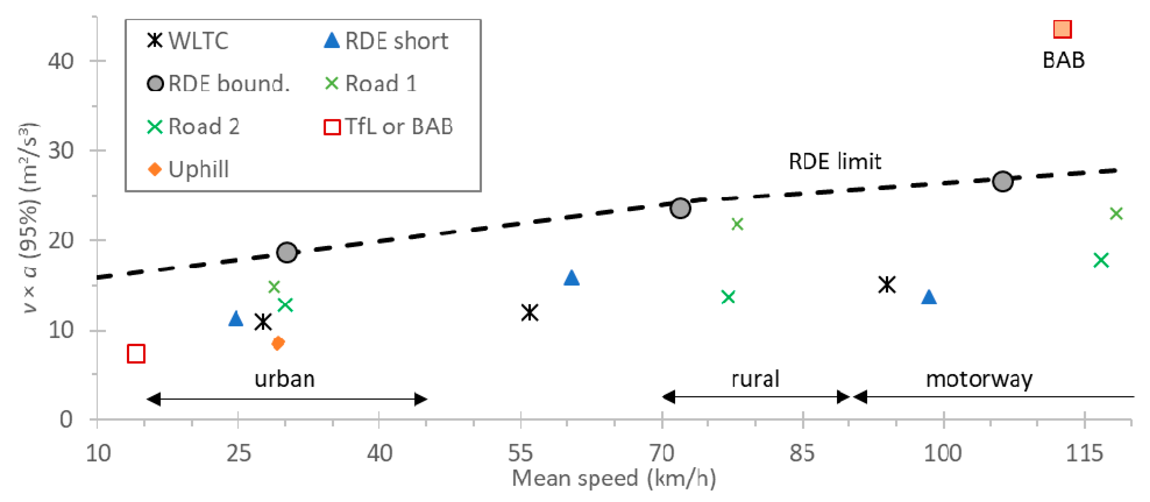
  • WLTC (worldwide harmonized light vehicles test cycle) Type 1 approval cycle. As urban part, the low and medium phases were considered, according to the RDE regulation, while the extra high phase was used as motorway part [44].
  • TfL (Transport for London urban interpeak) urban driving characterized by stop and go traffic in congested conditions. The cycle was developed by Millbrook Inc. in collaboration with the Traffic for London Authority [45].
  • BAB 130 (Bundesautobahn, Federal highway) high speed driving on the motorway up to 130 km/h, with frequent and sharp accelerations. It was developed by ADAC (Allgemeiner Deutscher Automobil-Club e.V.) as part of the EcoTest car testing protocol [46].
  • RDE short: A one-hour duration test with urban (time share 53%), rural (28%), and motorway conditions (19%), and road slope (range −9.6% to 9.2%) was provided by Ricardo Automotive & Industrial.
  • RDE boundary: A two-hour cycle recreating the most dynamic drive possible within the RDE boundaries with a 90% payload, including road slope (range −8.1% to 6.5%), provided by FEV Europe. The urban/rural/motorway time shares were 66%/20%/15%.
  • Uphill: A cycle (vehicle speed < 60 km/h) simulating (i) uphill driving with a 5% constant slope, while towing a 800 kg trailer (uphill tow); (ii) uphill driving with a 5% constant slope, car loaded to 85% payload and towing a 1700 kg trailer (85% of max trailer weight) (uphill tow 85%). The cycle was based on actual uphill driving data at the JRC premises.
  • RDE road: Two different routes according to Type 1A on-road procedure (RDE road) with a portable emissions measurement system (PEMS) (MOVE from AVL); routes were actually driven on the road at the JRC premises.
The WLTC tests were conducted using the test mass and roadload coefficients declared on the CoC (Certificate of Conformity) of the vehicle, after roadload derivation on the dyno. For the other cycles, the dyno coefficients were adjusted depending on the simulated conditions (e.g., slope, extra weight, etc.). The 95th percentile of the product of vehicle speed per positive acceleration greater than 0.1 m/s2 (v × a) for urban, rural, and motorway shares is plotted in Figure 1.
Ambient temperatures tested were −30 °C, −10 °C, −7 °C, 5 °C, 23 °C, and 50 °C for the TfL, BAB, and RDE short cycles. The RDE boundary and the uphill cycles were driven at −7 °C and/or −10 °C, as these were considered the most challenging situations at or slightly above the permitted RDE boundary conditions. The WLTC test temperature was 23 °C, as required in the regulation, while the ambient temperature during the on-road tests was 1720 °C. Temperatures of −30 °C and 50 °C were selected because these conditions are far from the normal operative conditions for which the vehicle might be calibrated. Note that such temperatures are not expected in Europe and compliance with any limits is highly unlikely.

3. Results

Initially, the laboratory type-approval Type 1 results are given, followed by real-time examples. Special attention will be given to cold start emissions. Then, urban and motorway emissions will be presented. Our focus is on regulated pollutants (CO, NOx, THC) and only NH3 from non-regulated pollutants. Other non-regulated pollutants were low for the specific vehicle (e.g., N2O < 3 mg/km). The emissions per km or kg of fuel can be found in the Supplementary Material.

3.1. Type 1 (WLTC) and Type 1A (RDE) Emissions

Table 2 summarizes the results for the on-road Type 1A (RDE), the laboratory Type 1 (WLTC), and the laboratory RDE-like cycles at different ambient temperatures. The WLTC emissions were three to six times lower than the respective Euro 6 limits applicable to the specific Euro 6d-Temp vehicle. The official tests (RDE road) were in agreement with the laboratory tests and much below the respective limit for NOx, where a conformity factor of 2.1 would be applicable for the specific vehicle to take into account the PEMS measurement uncertainty [47].
Various short (1 h) RDE-like cycles, which were not RDE compliant due to their short duration, at different temperatures also had emissions below the respective limits (although not applicable). The only exception was the −30 °C test, which had CO just at the Euro 6 limit, and THC 27% higher than the applicable limit at 23 °C. All these tests at −30 °C and −10 °C (and 50 °C) were outside the boundaries of the RDE regulation. The RDE at the boundaries (−10 °C, 90% payload, and dynamic driving at the limits of RDE) was also within the emission limits.
It should be mentioned that a correction of 1.6 would be applicable to emissions on RDE cycles at extended conditions (−7 °C to 0 °C, 30 °C to 35 °C) if the emissions calculation method was conducted according to RDE regulation (EU) 2017/1151. This correction was not applied to our analysis. Furthermore, an “RDE evaluation factor” should be applied at each test. It is calculated as the ratio of the test (trip) CO2 and the type-approval cycle CO2, and takes into account the severity of the trip. For ratios < 1.3, no correction is applied while, for ratios > 1.5, the inverse of the ratio is applied to the final emission result. For the specific vehicle, which was type-approved before January 2020, the respective ratios were 1.2 and 1.25. Again, no such corrections were applied to the results presented in this study. With such corrections, the results of the −30 °C would be well within the emission limits.

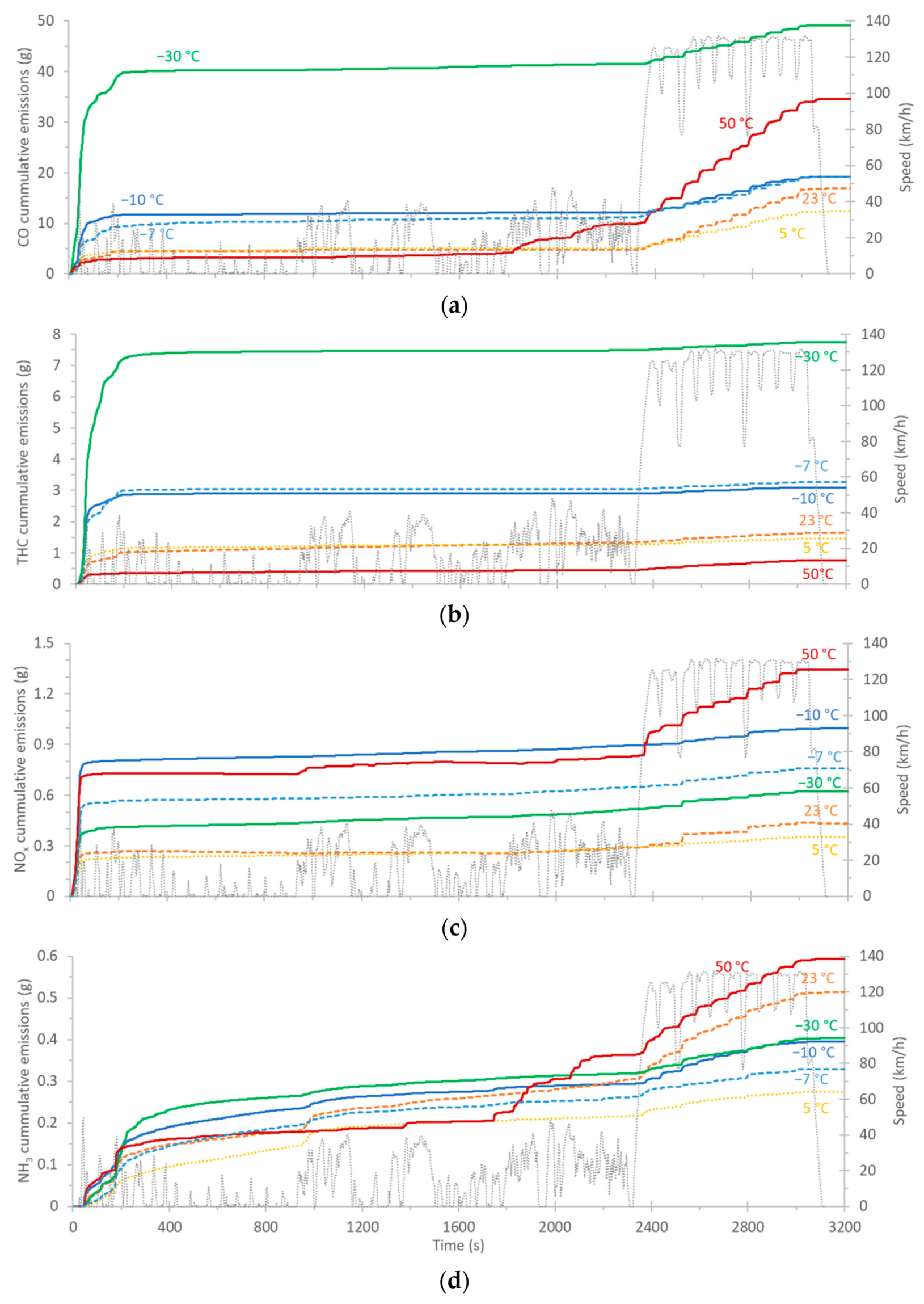
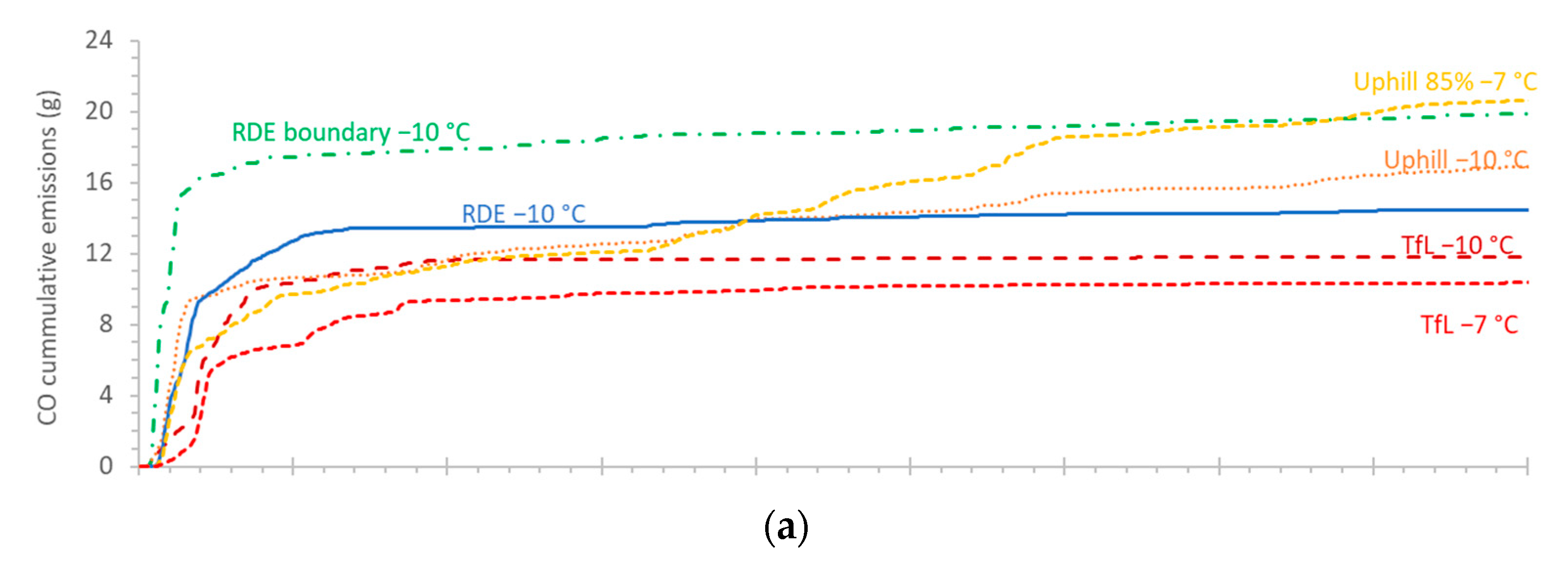
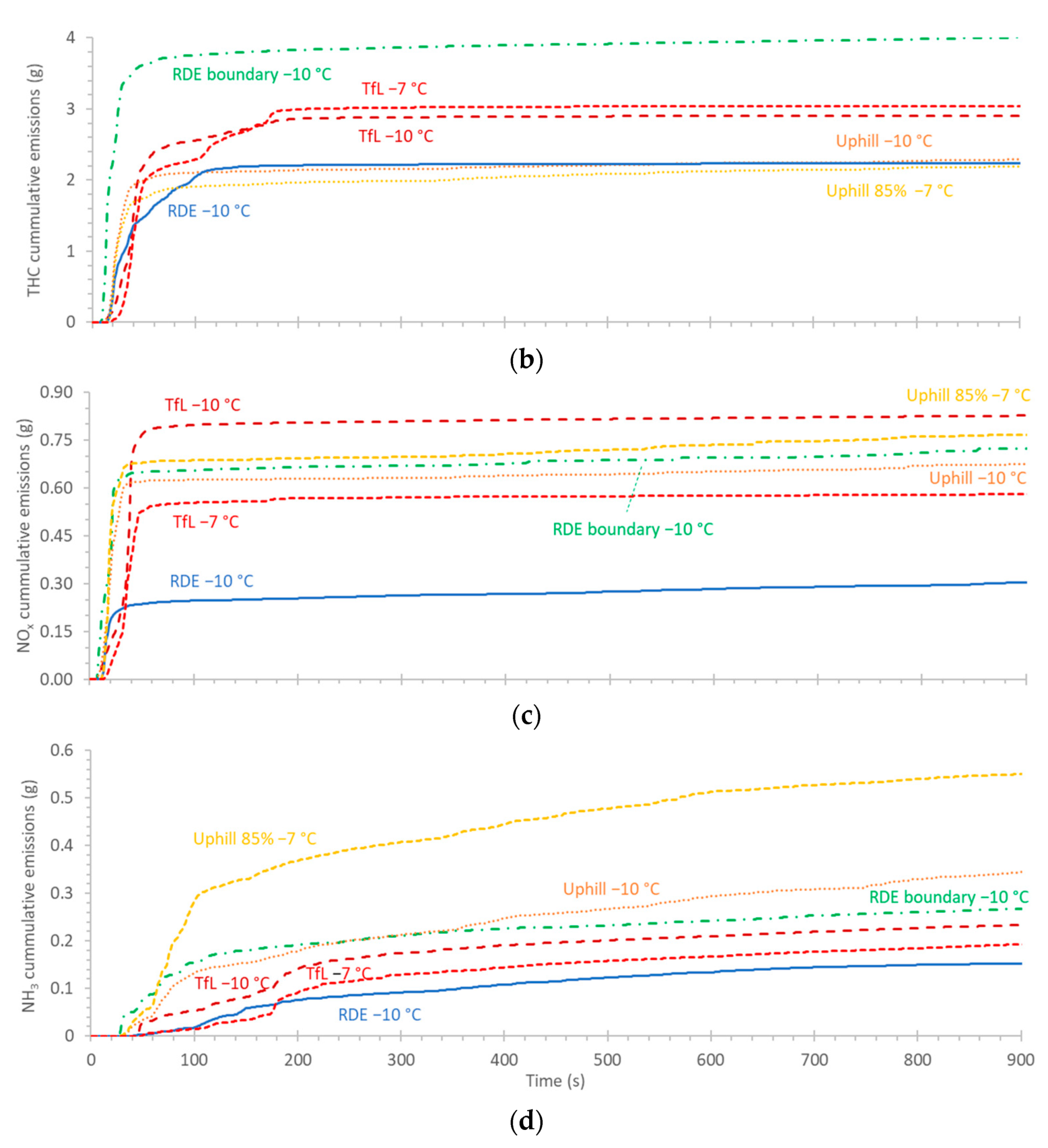
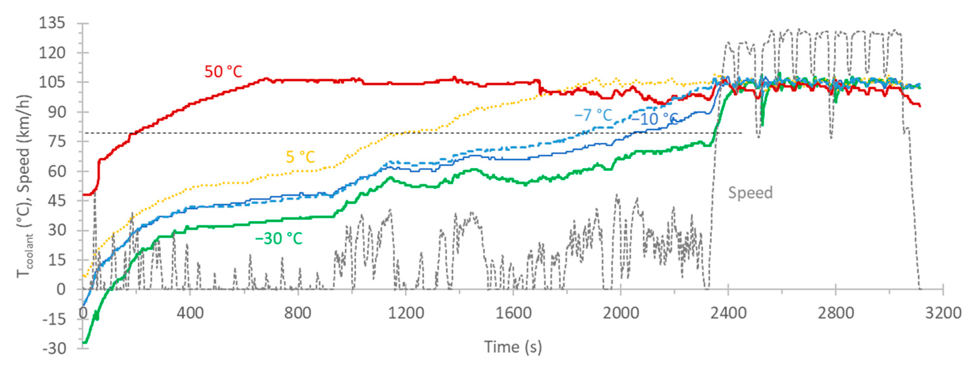
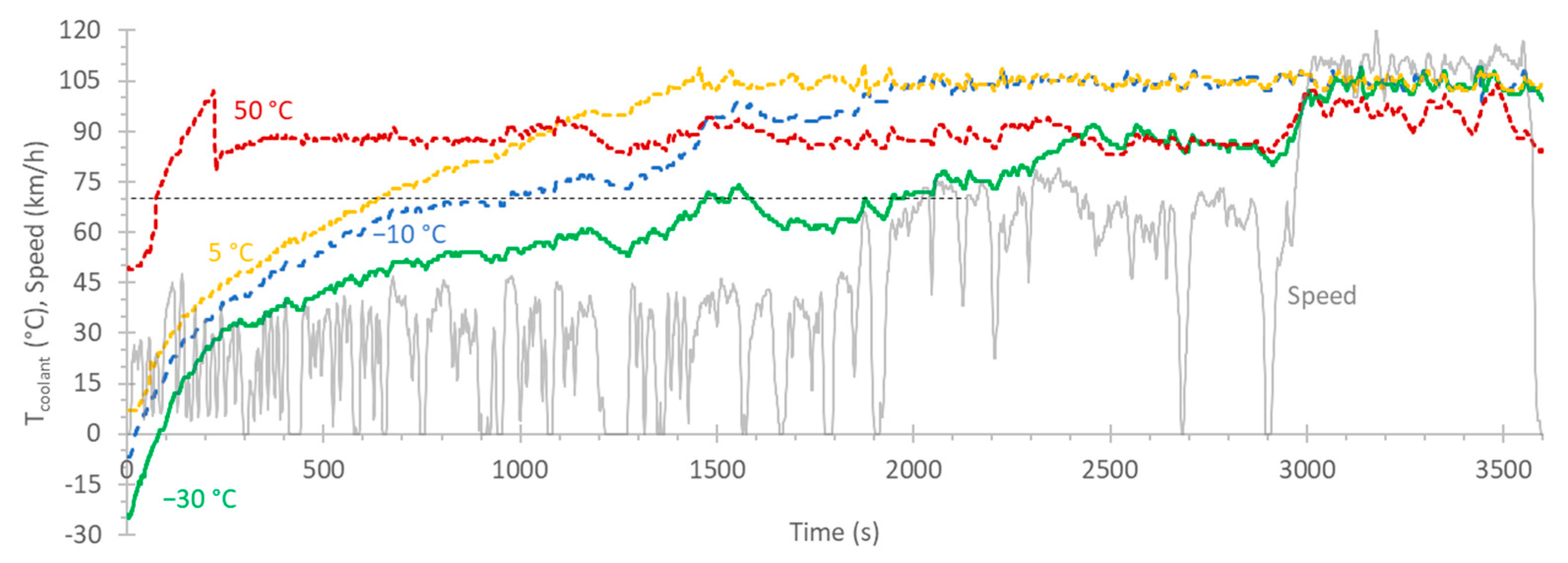
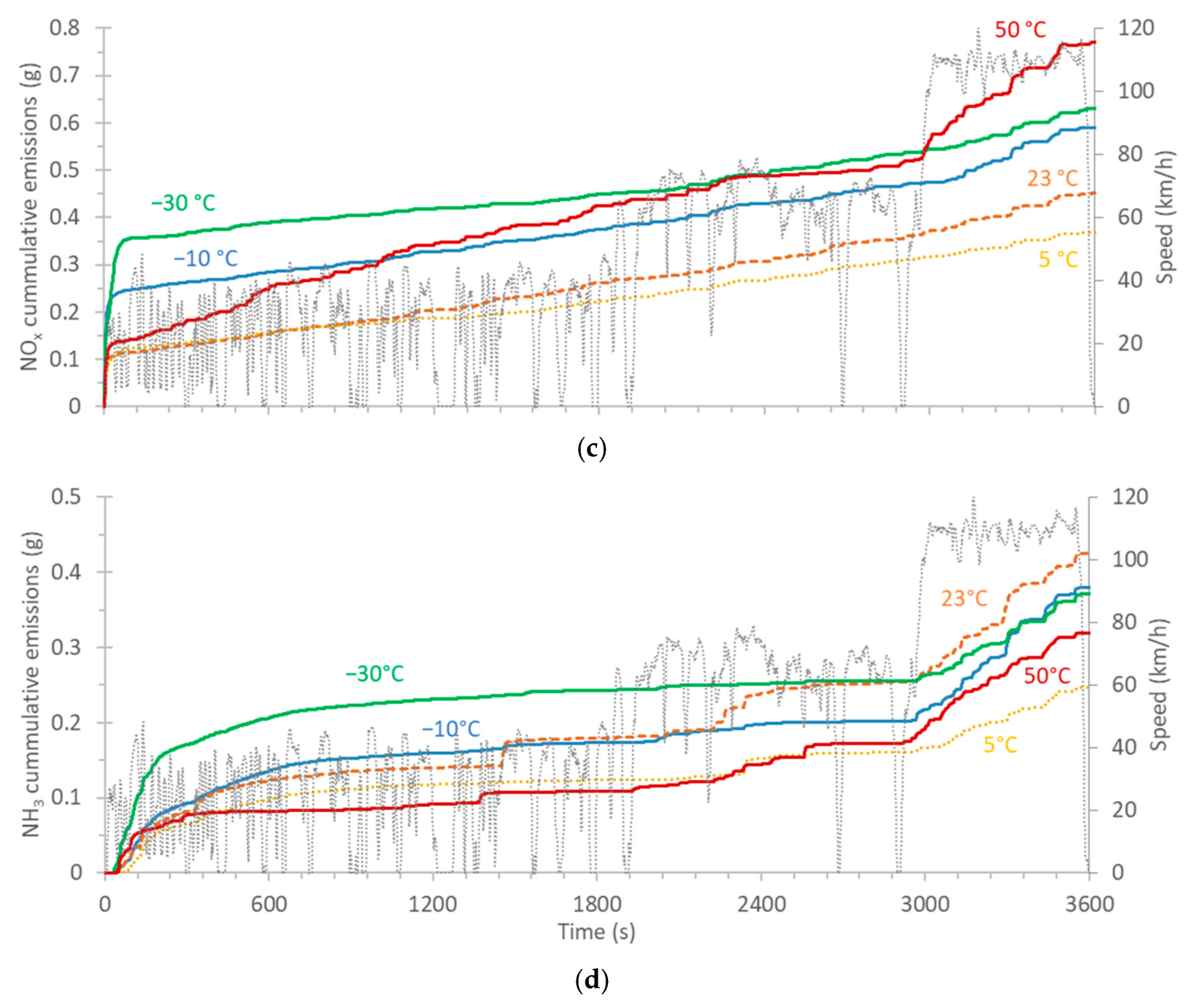
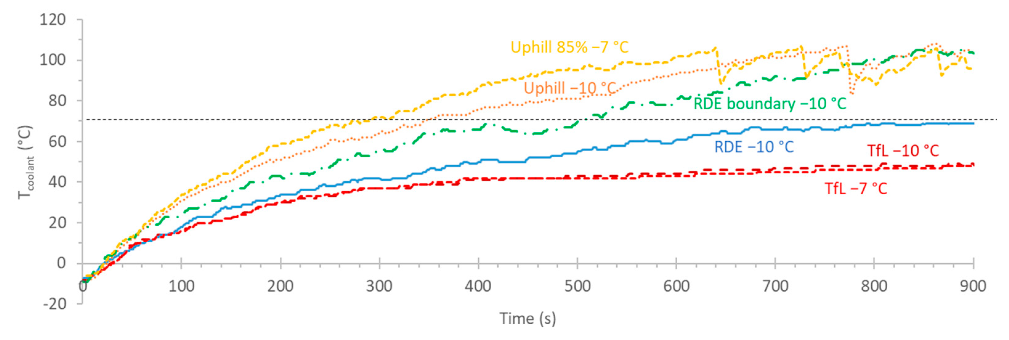
3.2. Real Time Examples

As an example, Figure 2 provides the speed profile and the cumulative emissions for the TfL (Transport for London) and BAB (Bundesautobahn, Federal highway) cycles for various ambient temperatures. More information regarding coolant temperatures can be found in Appendix Figure A1. The temperature profiles indicate a different engine thermal management strategy after 1700 s for the 50 °C test. There was no additional information available about air-to-fuel ratios or TWC temperatures. Exhaust gas temperatures can be found in the companion paper.
Figure 2a shows cumulative CO emissions. CO cold start emissions were higher for lower ambient temperatures. After the first minute (three minutes for −30 °C), the cumulative emissions remained almost constant until the motorway BAB cycles. The dynamic accelerations of the BAB contributed substantially less than the cold start emissions of the extreme low temperature (−30 °C), were comparable to the cold start emissions of low temperatures (−10 and −7 °C), more than the cold start emissions of mild temperatures (23 and 5 °C), and substantially more than the cold start emissions at high temperature (50 °C). Similar behavior was also seen for THC (Figure 2b) and NOx (Figure 2c). While ambient temperature had a clear effect on cold start emissions for CO and THC, this trend was not clear for NOx. For CO and NOx, there was a clear increase in emissions during accelerations, but not for THC.
NH3 emissions (Figure 2d) followed a similar trend. Although there was an increase during cold start, the step increase was noticed at 200 s, after the catalyst had reached its light-off temperature (as indicated by the stabilization of the cumulative emissions for the regulated pollutants). Increased emissions during the accelerations of the BAB cycle were also noticed.
In general, cumulative emissions stabilized much faster than the coolant temperature (compare with Figure A1), indicating that the TWC reached its efficient operating temperature faster than the engine. Of particular interest was the increase in emissions (in particular CO and NH3) at the last part of the 50 °C TfL test (around 1700 s), which coincided with the coolant temperature decrease which indicated a different engine thermal management.
The trends were similar for the RDE short cycles. After the cold start increase, cumulative emissions were flat (or smoothly increasing) at the urban part, and then increased slightly at the rural part and increased significantly at the motorway part. Examples are given in Appendix Figure A2 and Figure A3.
Figure 3 plots the cumulative emissions during the first 15 min for the various urban cycles. Figure A4 in the Appendix plots the coolant temperatures (no TWC temperatures were available). Most of the emissions of the urban part took place during the first one–two minutes, with a few exceptions. For the TfL at −7 °C, it took three minutes to reach a “plateau” in CO cumulative emissions (Figure 3a). Another notable exception was uphill driving with a simulated trailer with an 85% of maximum payload, where the CO emissions continued to increase almost linearly after the first two minutes (Figure 3a). The dynamic RDE boundary had the highest cold start CO emissions. THC emissions (Figure 3b) showed a similar trend, with the exception that uphill driving did not further increase the emissions after the first minute. Similarly, for NOx, after the first minute, the cumulative emissions were constant (Figure 3c). Uphill and dynamic driving had similarly high emissions, while the short RDE was the lowest. For NH3, as mentioned before, the increase appeared after the catalyst light-off, with the highest increase taking place somewhere between 80 s and 180 s (Figure 3d). The emissions continued to increase after the first three minutes. The highest emissions were noticed in uphill high load driving, followed by the dynamic cycle.

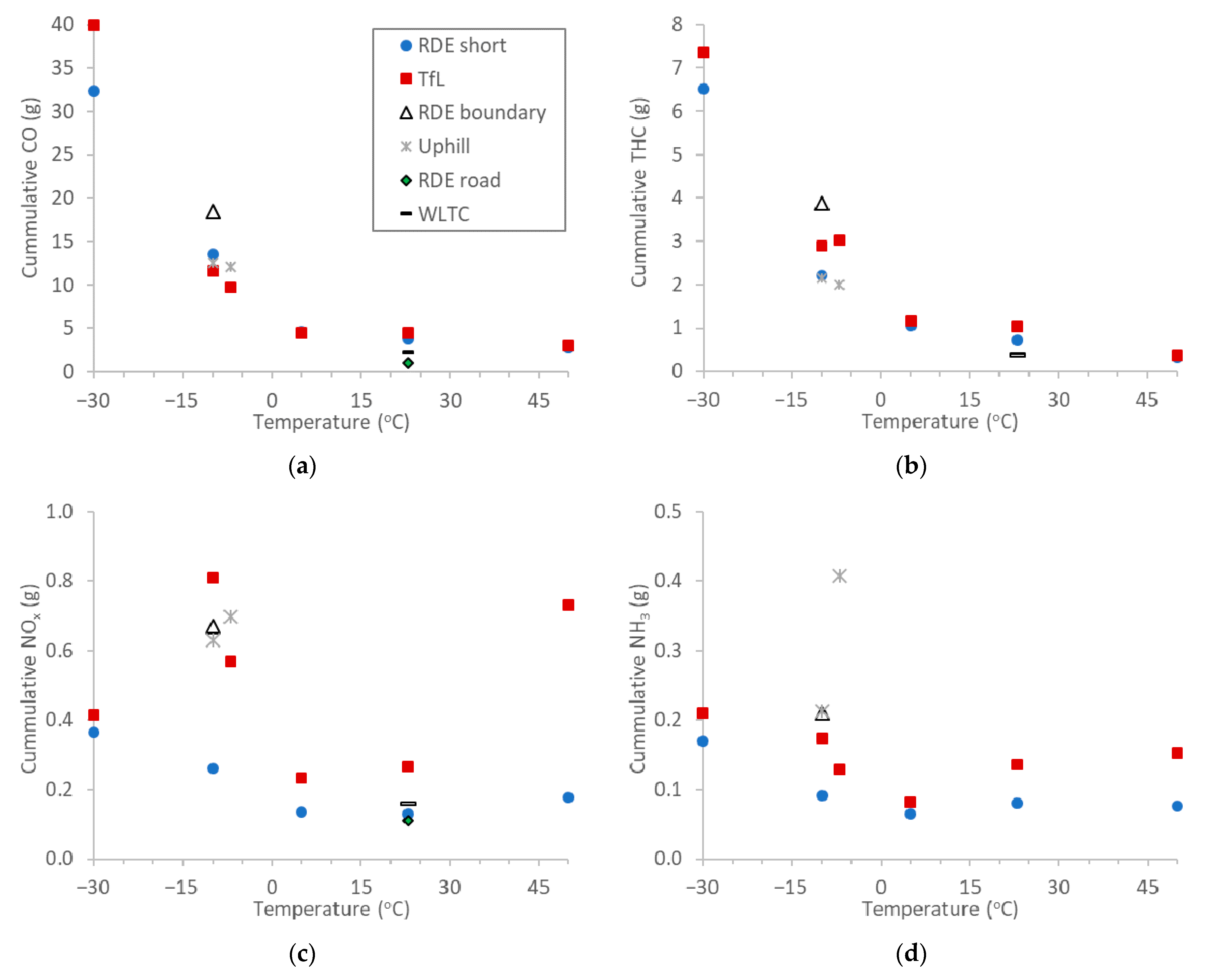
3.3. Ambient Temperature and Cold Start Emissions

Figure 4 summarizes the cumulative emissions (in g) during the first 300 s of cold start test cycles at various ambient temperatures. A duration of 300 s was selected in order to ensure the “plateau” region was reached (i.e., a small increase in the emissions afterwards), even in the extreme case of the −30 °C for the great majority of test cycles and pollutants, as presented in the previous section. For the other temperatures, the plateau region was reached within one to two minutes (see also Figure 2 and Figure 3). Furthermore, a cold start in the RDE regulation is defined as the first 300 s. The distance driven in the first 300 s varied from 1 km (TfL) to 2.8 km (uphill and RDE boundary). In the case of the RDE, the distance covered was 1.7 km.
There is a clear increasing trend with decreasing ambient temperature for CO and THC emissions (Figure 4a,b). The cold start (i.e., first 5 min) CO mass was <4.5 g at temperatures <5 °C, 10–18 g at −10 °C and 32–40 g at −30 °C. For the same temperature (−10 °C), the dynamic RDE boundary cycle had the highest emissions.
The cold start THC mass was <1 g at temperatures above 5 °C, 2–4 g at −10 °C and 7 g at −30 °C. For the same temperature (−10 °C), the dynamic RDE boundary cycle had the highest emissions. At low ambient temperatures, the TfL had higher emissions than the RDE short.
For NOx, the trend in function of temperature was less evident, and the emissions had a bathtub-like curve, especially in the case of the TfL cycle; high emissions were seen at both low and high temperatures, and the TfL was higher than the RDE short (Figure 4c). The dynamic RDE boundary and the high load uphill cycles also showed high emissions. Comparing the CO and NOx graphs (e.g., for TfL), the NOx–CO trade-off related to lambda control could be seen; when CO was high, NOx was usually low, and vice versa.
For NH3 (Figure 4d), the temperature dependence was almost non-existent. For a specific temperature, there was an influence of the cycle: (i) the dynamic cycle had high emissions; (ii) the stop and go TfL had higher emissions than the moderate RDE short; (iii) the high load uphill cycle had high emissions (~140 mg/km over the first 2.8 km).

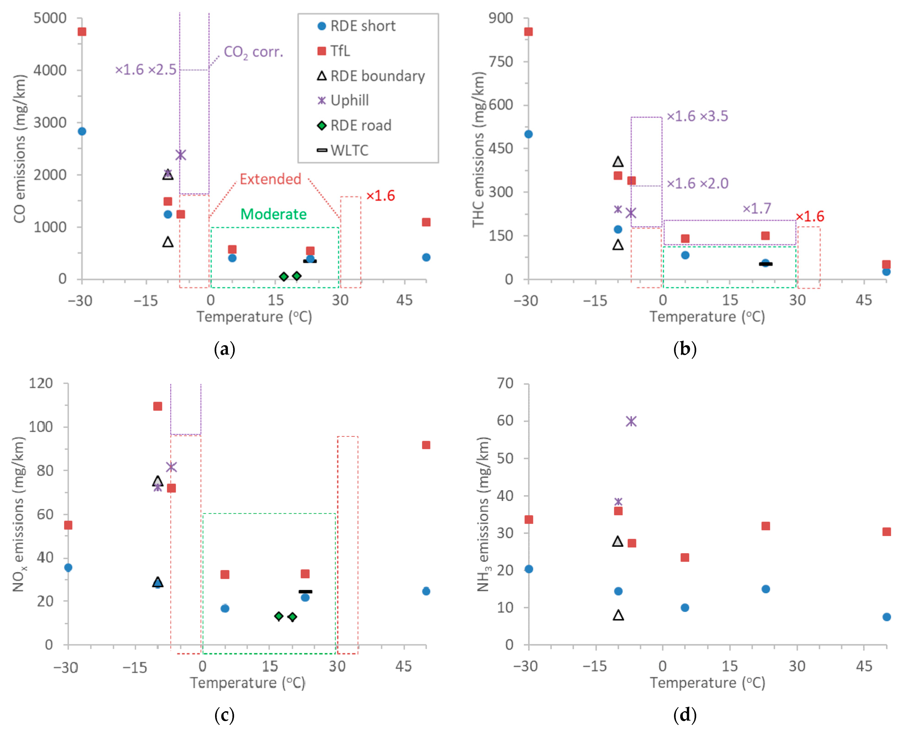
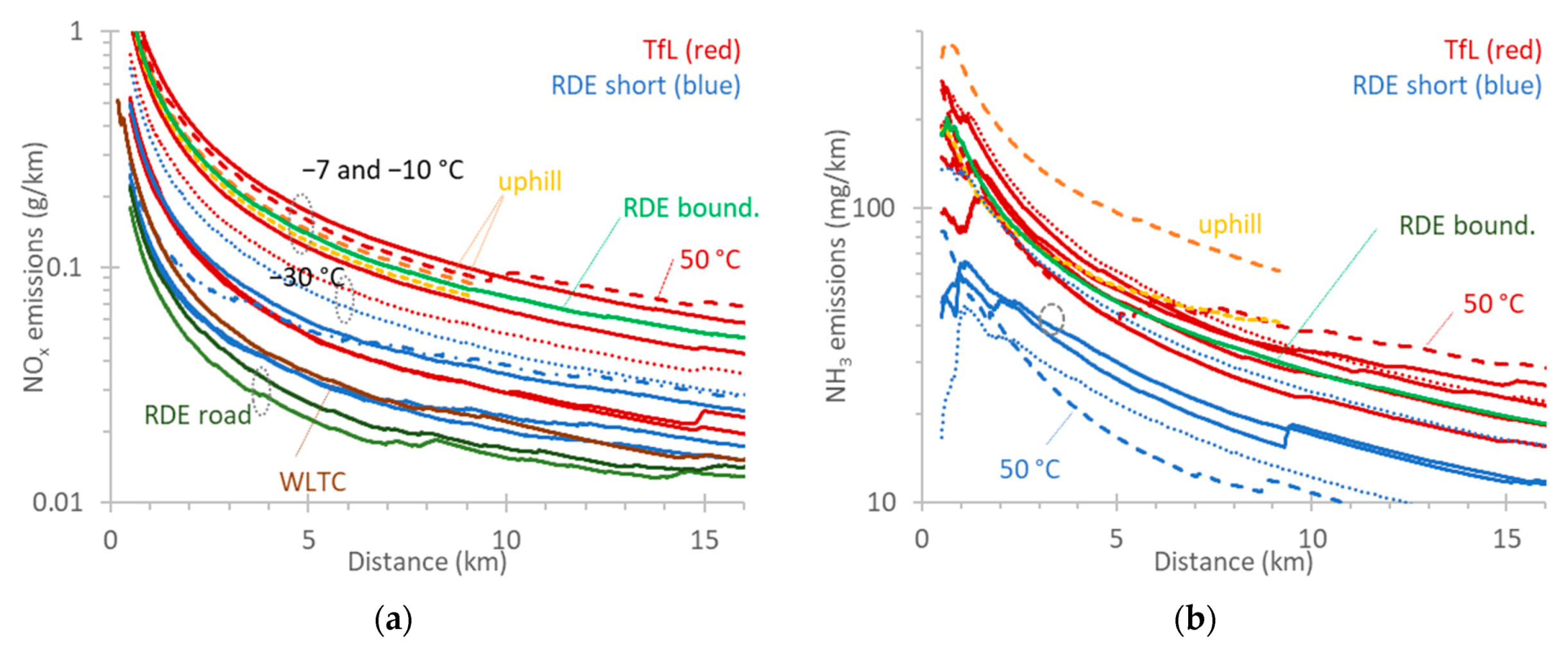
3.4. Ambient Temperature and Urban Emissions

Figure 5 presents the emissions (in mg/km) of the vehicle for the urban cycles and urban parts of the rest cycles. The TfL was an 8.9 km urban cycle and the urban part of the RDE short urban cycle was 12.7 km, while the urban parts of the dynamic RDE boundary and actual RDE on-road cycles were around 35 km long. The uphill cycles were 9 km long, representing uphill driving towing a trailer with 85% of the maximum weight. The WLTC low and medium part were 7.8 km long. It should be recalled that the minimum urban distance in the current regulations is 16 km; thus, any comparison with limits of non-RDE compliant tests (e.g., TfL, uphill) is only for illustrative reasons.
To put the results into context, the RDE limits were also plotted for moderate conditions (0 °C to 30 °C) (shown as a green box). At the extended conditions of the RDE (−7 °C to 0 °C, 30 °C to 35 °C), a 1.6 correction factor should be applied to the emissions. Here, instead of reducing the emissions with this factor, we increased the moderate limit (adjusted limits shown as red boxes) for better visualization and to leave the actual emissions of the vehicle intact. In addition to this correction to the emission limits (red box), the RDE evaluation factors (CO2 corrections) were plotted as purple boxes. For urban trips the on-road, CO2 was divided by the CO2 of the L + M phases of the WLTC. For our tests, the ratios were 1.4–1.9 for the RDE short urban and 1.7–2.5 for the TfL. The higher values were for the low temperature and high temperature tests. For the uphill driving cycles, the ratios were 2.8–3.5, confirming the high-power demand of the specific cycles.
For NOx measured on the road with PEMS, a conformity factor of 2.1 was applicable to the specific Euro 6d-Temp vehicle [47]. The conformity factor for Euro 6d vehicles is 1.43 and will be lowered in the future. The other gaseous pollutants have no conformity factors because they are not yet regulated and verified on the road. As all our tests were conducted on the chassis dynamometer with laboratory grade equipment (except RDE road), no conformity factor was applied, and all results were compared with the laboratory limits.
The results are quite similar to Figure 4. The reason for this is that, for the urban section of the tests, most of the emissions are produced during the first minutes, so any difference is mainly due to the different length of the urban cycle.
The CO emissions (Figure 5a) from 550 mg/km at moderate conditions increased up to 2400 mg/km at the uphill cycles at −7 °C and 4700 mg/km at the TfL at −30 °C. At 50 °C, CO was 1100 mg/km. The TfL emissions were, in general, higher than the short RDE, with the differences increasing at the extreme temperatures. The RDE boundary was lower than the rest cycles, but the urban distance was three times longer. Considering only the first 10 km, the emissions were 2000 mg/km, close to the uphill cycles, which had the highest emissions at the same ambient temperature (−7 °C or −10 °C).
The THC emissions (Figure 5b) showed an increasing trend with decreasing ambient temperature. From 50 mg/km at 50 °C and 50–150 mg/km at 5–23 °C, they reached 150–400 mg/km at −10 °C and 500–800 mg/km at −30 °C. The loaded uphill cycles were between the TfL and short RDE, while the RDE boundary had the lowest emissions for the same temperature (or the highest when considering only the first 10 km). CH4 emissions (no figure shown) were generally <10% of THC emissions (20% for THC <20 mg/km). Percentages around 30% were measured for the RDE boundary and TfL at positive ambient temperatures.
The NOx emissions showed a bathtub-like curve in function of the ambient temperature (Figure 5c). They ranged from 10 mg/km to 35 mg/km at the 5–23 °C region, and up to 70–110 mg/km at −10 °C or 50 °C on the TfL cycle. The high load uphill cycles at −10 °C were also around 80 mg/km. However, emissions were kept at 30 mg/km at −10 °C for the urban part of the short RDE and the dynamic RDE (but at 75 mg/km considering only the first 10 km). Interestingly, they were <55 mg/km at −30 °C for the same cycle (RDE short).
The NH3 emissions (Figure 5d) were relatively constant for different temperatures. High ammonia emissions (30 mg/km) were measured at the TfL, irrespective of ambient temperature and the uphill towing cycles (40–60 mg/km). The RDE boundary also had 30 mg/km when only the first 10 km were considered. Lower levels (10–20 mg/km) were measured with the RDE short. Currently, there are no limits on this pollutant. For TfL, the average 35 mg/km NH3 emissions resulted from slightly less than 20 ppm average NH3 concentrations, with peaks of 200–400 ppm during the first minutes.
The N2O emissions (no figure shown) were <3 mg/km, except for the TfL tests, which were around 5 mg/km; these were always confined to the temperature window of the catalyst light-off.

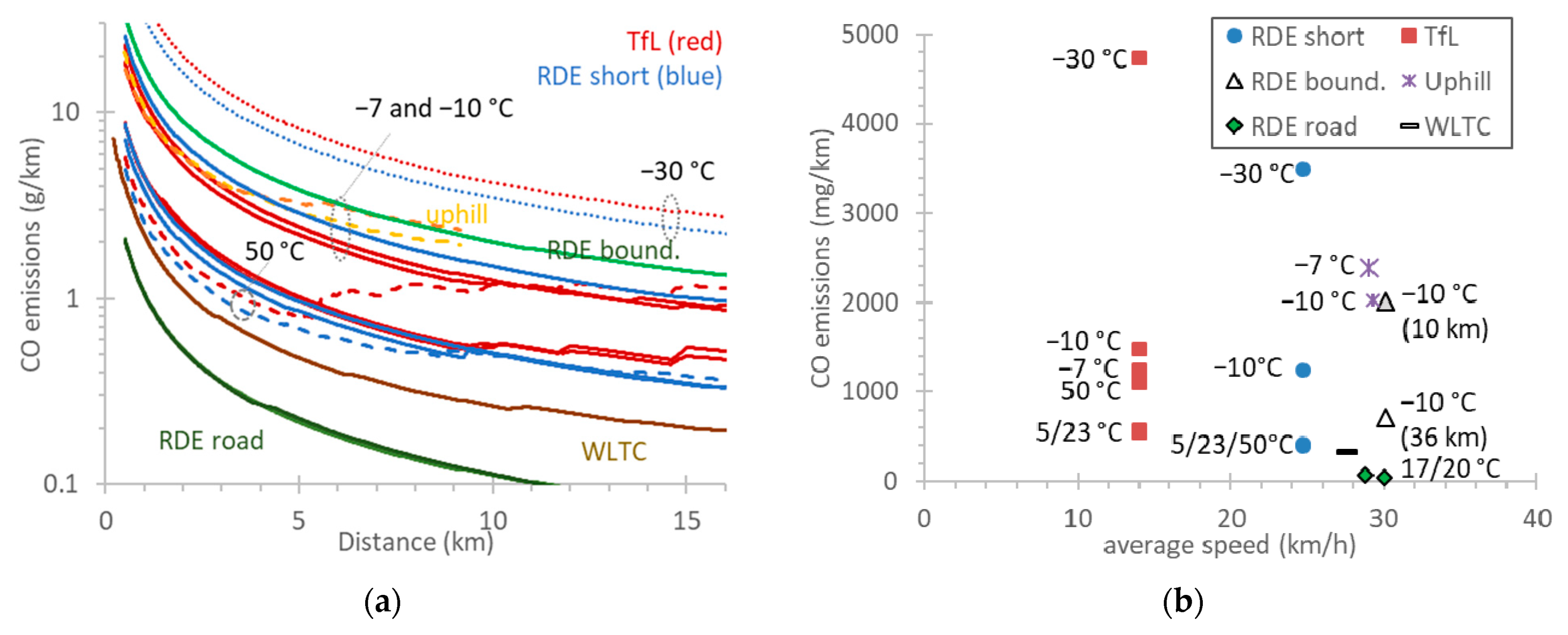
3.5. Ambient Temperature and Motorway Emissions

Figure 6 summarizes the emissions during the motorway cycles at various temperatures. The distances were 8.3 km (WLTC), 19.1 km (RDE short), 25 km (BAB), and 29–34 km (RDE road, boundary). There are no limits applicable only for the motorway part; thus, only the complete RDE limits at moderate conditions (0–30 °C) are given in green boxes for illustrative purposes.
CO emissions (Figure 6a) were approximately 400 mg/km, with the exception of the RDE boundary at −10 °C and the cycles at 50 °C, where the emissions reached 1000 mg/km (still below the laboratory limit, even though they were not applicable). The THC (Figure 6b) were below 20 mg/km in all tests, except at the RDE boundary, where they reached 35 mg/km. At the RDE boundary, THC spikes were evident in the motorway part, but the emissions were still three times below the laboratory limit of 100 mg/km. The NOx emissions (Figure 6c) were only 5 mg/km, reaching 20 mg/km in the BAB cycle at 50 °C. The dynamic RDE boundary at −10 °C had 15 mg/km. All results were lower than the (non-applicable) limit of 60 mg/km. The NH3 emissions (Figure 6d) were below 10 mg/km for all cycles and temperatures.

4. Discussion

This study assessed the emissions of a Euro 6d-Temp gasoline vehicle with a close-coupled TWC and an underfloor uncoated GPF, focusing on extreme temperatures and driving conditions. The results confirmed previous findings, i.e., (i) during urban operation, the majority of emissions comes from cold starts; (ii) the lower the ambient temperature, the higher the cold start emissions, namely for CO and THC (not so evident for NH3); (iii) dynamic driving and/or high engine load increase the emissions of most pollutants. The major contribution of this study is the extension of these findings to extreme ambient temperatures (−30 °C and 50 °C) and driving conditions (traffic, dynamic driving, trailer towing).

4.1. Cold Start

Higher emissions during a cold start are known and attributed to higher engine-out emissions and low efficiency of the aftertreatment devices [48,49,50]. It was shown that, even though it took long time for the coolant temperature to stabilize, the cumulative emissions, in most cases, stabilized within a few minutes; this highlights the importance of aftertreatment devices’ status on tailpipe emissions, which is in agreement with other studies [51]. Cold start emissions, defined here as emissions in the first 300 s (and not the difference between cold and hot start emissions [52]), contributed, in many cases, >80% of CO, THC, and NOx urban emissions (Table 3). For CO, the contribution was lower in the 50 °C tests and the high load uphill towing cycles because there were also considerable emissions during the rest of the urban phase. For NOx, the contribution was lower in most RDE short tests. Other studies have also found a high contribution from cold start for CO (>70%), but this is smaller for NOx (40–60%) for turbo-charged GDI vehicles [53,54,55]; however, lower percentages have also been reported for RDE trips [32,56].
The cold start contribution was around 50% for NH3. NH3 has been shown to primarily form within the exhaust temperature range of 250–550 °C [57]. NH3 formation over the catalyst is enhanced at low air/fuel (lambda) ratios (rich operating conditions). The mechanisms that take place under these conditions are the water–gas (CO) shift reaction, producing H2 and the reaction of NO and H2 [58]. The availability of H2 and CO, the exhaust gas temperature, and the lambda also affects small differences in the slopes of the cumulative NH3 functions between different temperatures [59].
Table 4 summarizes the contribution of a cold start to total RDE trips. In general, the contribution was <50% for CO and NOx, <25% for NH3, but >50% for THC. Higher percentages were measured at lower ambient temperatures. For the actual on-road tests, the contribution was 6–19% for CO and NOx, which is in agreement with other studies [56,60].

4.2. Urban Emissions

The urban emissions of the regulated pollutants (CO, THC, NOx) were primarily determined by cold start emissions. As the contribution of the hot urban operation was small for most pollutants, a longer distance resulted in lower distance specific emissions. The emission factors presented in Figure 5 were quite comparable because the urban distances were within 9–12 km. Figure 7a presents the emissions in function of distance. CO is plotted as an example. Each cycle is plotted with a different color. Different groups of curves can be seen; the highest emissions are at −30 °C, followed by the −7 °C and −10 °C tests. The other group is the 5 °C, 23 °C, and 50 °C tests. For each group of temperatures, TfL emissions are usually higher than the RDE short (primarily NOx and NH3). RDE boundary emissions are higher than the other cycles; the RDE road and WLTC are lower than the rest cycles. What is important from this figure is the decreasing trend in emissions (note the log scale) in function of distance, with a few exceptions: the uphill cycles and the 50 °C tests, as discussed before (Figure 3). Thus, for pollutants for which the cold start contribution is important, total distance of the urban cycle is also important. For NOx (Figure 8a), the highest emissions were noted for uphill, RDE boundary, and TfL (all cycles at −7 °C or −10 °C), as well as TfL at 50 °C. For NH3, the highest emissions were seen for uphill with an 85% payload (car and trailer) (Figure 8b).
Many studies plot emissions in function of the average speed [29,61] because, typically, a decreasing trend is expected for low average speeds. As an example, Figure 7b plots CO emissions in function of the average speed for different urban cycles. The typical curve, where emissions increase as average speed decreases, is not so evident. Ambient temperature, dynamic driving, high load, and total distance all have a bigger influence. For the other pollutants, the results are similar, and the average speed dependence is even smaller. Such a lack of correlation was also shown recently for vehicles fulfilling China 3 to China 5 emission limits [62].

4.3. Ambient Temperature

Higher emissions due to lower ambient temperatures are well documented [22,30,63,64,65]. High viscosity and friction are the primary causes of emission increases; excess fueling is also important [66]. The use of air conditioning can also contribute to an increase in emissions, even at low temperatures, due to the increase in engine load (and possibly richer fuel injection, injection pressure, and delayed spark timing) needed to operate the compressor and/or fan of the air conditioning [67,68]. In our study, the air conditioning of the vehicle was always enabled at 21.5 °C. At lower ambient temperatures, the TWC can take longer to reach the light-off temperature [29] and/or the lambda is not kept in unity. In this study, it was shown that, even in the extreme temperature of −30 °C and the challenging traffic cycle of TfL, the TWC could operate efficiently within <300 s. Table 5 summarizes the emission ratios at various temperatures compared to 23 °C for TfL (cold start, urban), BAB (motorway), and the RDE short (cold start, urban, motorway).
CO cold start emissions at −7 °C of Euro 4 vehicles have been shown to be 15–45 g [69]; cold start values are between 6 and 32 g for Euro 5 [34,70] and at an average of 27 g for China 6 GDI [10]. However, in our study, they were 10–15 g. At −20 °C, the cold start emissions of the Euro 4 vehicles were 50–160 g [69] while, in our study, they were 32–40 g at −30 °C. Distance specific emission factors of four Euro 6 GDI vehicles were 1.3–8.0 g/km (over the first phase of WLTC) [30], while four Euro 6b GDI vehicles emitted 5–12 g/km at the urban Artemis cycle at−7 °C [35]. These values are, in general, higher than the 1.5 g/km found in our study, confirming that the vehicle of our study was one of the best vehicles in terms of emissions. Both the absolute levels and the ratio of the −7 °C to 23 °C cold start emissions were on the lower side of reported values. In our study, this value was close to 3 (Table 5), while typical factors of 4–5 were reported [35,66,70], and sometimes even >8 [35,66,69,71].
Similarly, THC cold start emissions at−7 °C for Euro 4 vehicles were 5–15 g [69]; cold start values are between 1–4 g for Euro 5 [34,70] and at an average of 3 g for China 6 GDI [10]. However, in our study, they were 2–3 g. The emissions increased by a factor of 2.5–3 compared to 23 °C, which is again lower than what is reported in the literature [35,66].
On the other hand, no clear effect of ambient temperature on NOx for gasoline cars is reported in the literature [17,35,56,69,72]. However, some studies report a relatively small increase [10,30,34]: At −7 °C, NOx emissions were, on average, 1.7 times higher than at 23 °C [30]. Higher NOx emissions from spark ignition vehicles may be related to lower catalytic efficiency and longer periods to reach light-off temperature at cold ambient temperatures [30]. On the other hand, at lower temperatures, combustion is usually rich, which results in relatively low NOx emissions. With rich mixtures, the catalyst promotes a reduction in NOx by reactions involving HC and CO [73]. Thus, it seems emissions reduction is highly dependent on the strategy of a given vehicle’s manufacturer.
NH3 emissions only marginally increased at lower ambient temperatures. This is in agreement with other studies, where NH3 emissions from Euro 6 vehicles increased on average 1.5 times while temperature decreased from 23 to −7 °C [30]; however, much higher increases have also been reported [70], which are probably due to enrichment. At higher than 23 °C, a study found an increase in NH3 emissions [74], while, in our tests, the increase was negligible. It seems that the parameters that increase NH3 (temperature and lambda) were well controlled by the vehicle of our study.
Studies at high ambient temperatures are scarce [17,74,75]. Tests with Euro 3 vehicles with air-conditioning switched on showed a clear increase in CO and THC emissions at 37 °C, but not for NOx. Another study did not find any effect on CO and NOx at temperatures up to 40 °C [74]. Here, we found no effect on CO and HC cold start emissions, but a clear effect on NOx was apparent. That said, we documented an effect on CO emissions of the motorway cycles. The differences compared to older studies can be attributed to better lambda control at high speeds with the vehicle of our study (for CO and THC) and/or correctly sized TWC (adequate space velocities for the highest exhaust flows). More fundamental studies in that direction are necessary to generate a deeper understanding.

4.4. Dynamic Driving

Dynamic driving had a clear effect on CO and THC. Aggressive driving resulted in deviations from stoichiometric mixture, affecting both engine-out emissions and TWC conversion efficiency. The dynamic driving effect was evident at both cold start and motorway cycles. In the urban cycles, it was less evident because the RDE boundary distance was more than three times longer than the rest cycles, resulting in distance-specific emissions at the same levels of the rest cycles. However, when the dynamic RDE boundary was calculated for the first 10 km, the emissions were clearly high. Higher emissions with dynamic driving for CO have also been reported by others [23]; typically, emissions increased by a factor of 3, but some vehicles increased by a factor of 30 on urban routes.
For NOx and NH3, the effect of dynamic driving was smaller, which is in agreement with other studies [76]. For these two pollutants, emission levels of the dynamic cycle were similar to the TfL or uphill driving cycles. Similar, or even reduced, NOx emissions with dynamic driving have been reported by others [77]; however, these typically increase by around 80% on urban routes [23]. A study showed that, during fuel-cut events, air oxidizes the catalyst. Then, the excess fuel during accelerations results in NH3 formation on the first part of the catalyst. When the rear part of the catalyst is not yet reduced, it oxidizes NH3 back to NOx [78]. Another study showed that the instantaneous peaks of v × a had a clear one-to-one correspondence with the peaks of instantaneous NOx emissions [53]. For the same route, higher v × a results in higher emissions [23,79] but, when different routes are compared, this is not necessarily true [41] because v × a does not take into account slope or additional weight.

4.5. Towing and Uphill Driving

The cycle including uphill driving and towing a trailer with 85% of the maximum payload had high cold start emissions, particularly NH3. The reason for is high engine-out emissions (not for NH3) and low conversion efficiency of the catalyst during the first minutes. In particular, for NH3, in the TWC, in addition to the NH3 coming from a rich operation, the high exhaust gas temperature favored the formation of NH3 from engine-out NO. The increasing trend in cumulative emissions also continued after the cold start, indicating rich engine operation due to the high power demand, as the TWC had already reached its operating temperature. We are not aware of similar tests, especially at low ambient temperatures of −10 °C.

4.6. Motorway Emissions

Total CO and NH3 presented non-negligible emissions during motorway operation. However, the motorway distance was higher than in urban operations, resulting in lower distance-specific emissions. Approximately 10 mg/km of NH3 emissions corresponded to slightly less than 10 ppm of average NH3 concentrations, with peaks between 50 and 100 ppm during accelerations. Similar levels have been reported by others [80]. In the case of NOx and THC, the contribution of the hot operation was small, and the long motorway distance resulted in low distance-specific emissions. Higher emissions were seen during dynamic driving for all pollutants (except NH3). Nevertheless, the emissions were still relatively low (i.e., below the laboratory or on-road limits, even though not applicable to the motorway part separately). High emissions were also seen at a high ambient temperature (50 °C) for CO and NOx. The combination of high loads and exhaust gas temperatures is typically addressed by fuel enrichment for component thermal protection, which increases fuel consumption and emissions [81]. Furthermore, it could be that the 50 °C condition had not been optimized and/or calibrated. Nevertheless, for this vehicle, there were no high CO and NOx emissions on the motorway, as has been reported in some other gasoline vehicles [22,23,82]; in our tests, emissions were always below the (non-applicable) limits. The high emissions in previous studies could be also due to the small catalyst volume (i.e., high space velocity at high speeds) [83] and a rich engine operation (both result in lower conversion efficiency).

4.7. Concluding Remarks

The emissions of the vehicle of this study were low compared to other vehicles of the same emission level (Euro 6d-Temp) or older (e.g., Euro 5 or Euro 6b), as has been discussed previously. For this reason, it cannot be considered necessarily a representative vehicle of the current fleet. Nevertheless, it would not meet the proposed Euro 7 limits by CLOVE [84]. For example, the 30 mg/km (or 480 mg up to 16 km distance) would not pass the TfL cycle (around 600–800 mg) at−7 °C. Similarly, at −7 °C, the NH3 emissions (10–20 mg/km) were higher than the proposed limit of 10 mg/km, and the CO emissions were almost double than the proposed limit of 600 mg/km, clearly indicating that future vehicles will need to be very clean.
As many researchers have shown, the majority of the emissions are emitted during the first minutes of a vehicle’s ignition [85]. Although there are differences in the absolute levels between different vehicles, the cold start still remains the main contributor in most cases, and it needs to be controlled better. Thermal management methods, such as those based on burners, reformers, and electrically heated catalysts, might further decrease cold start emissions, and a degree of electrification might be necessary [27,86,87,88,89]. However, in some cases, urban emissions of hybrid electric vehicles might be higher due to the longer time needed for the catalyst to warm up; thus, further calibration efforts are needed [32,90]. Furthermore, keeping the TWC temperature and lambda value at appropriate levels in urban stop-and-go traffic situations will be important. The difficulty of controlling cold start emissions does not mean that the rest trip is not important. It was shown that the motorway section can have an equal or even higher contribution in mass (g), even though it was relatively low as mass per distance in the vehicle used in our study. However, this is not always the case [22]. A pollutant that requires attention is NH3. In most cases, emissions were around 10 mg/km but, at urban cycles, they reached 35 mg/km. These levels are higher than the US limit of 6.2 mg/km and, in some cases, higher than the China limit of 20 mg/km (applicable to different cycles).
One important topic that was not addressed in this study is the catalyst’s deactivation and deterioration over time [91]. The performance of a catalyst degrades over its lifetime through several mechanisms, including precious metal agglomeration, washcoat breakdown, as well as selective and non-selective poisoning. Thus, emission levels close to the useful life of a vehicle also need to be studied in the future. Finally, the effect of fuel on emissions also has to be considered.

5. Conclusions

A Euro 6d-Temp gasoline vehicle with TWC (three-way catalyst) and GPF (gasoline particulate filter) was tested on the road with the Type 1A on-road real driving emissions (RDE) procedure (at 17–20 °C), as well as in a laboratory with the Type 1 worldwide harmonized light vehicles test cycle (WLTC) (at 23 °C). Additional urban, motorway, dynamic, and uphill driving cycles with different payloads were conducted in the laboratory at temperatures between −30 °C and 50 °C. This is one of the few studies that has assessed a low-emitting vehicle at extreme temperatures and in extreme driving conditions.
Maximum emissions at motorway cycles at 23 °C were 500 mg/km for CO, 10 mg/km for THC, 5 mg/km for NOx, and 9 mg/km for NH3. Maximum emissions at the congested traffic urban cycle (TfL, 8.9 km long) at 23 °C were 550 mg/km for CO, 150 mg/km for THC, and 32 mg/km for NOx and NH3. At −10 °C, urban emissions were around two times higher for CO, HC, and NOx, and at the same levels for NH3. The first 300 s contributed >75% to CO and HC and 45–90% to NOx and NH3 of urban emissions, depending on the cycle and the ambient temperature. Compliance with the proposed future Euro 7 limits will require further emission reductions, especially at a cold start. More fundamental studies (i.e., measurement of air/fuel ratios, catalyst temperatures, etc.) are needed to better understand the behavior of vehicles in such conditions.

Supplementary Materials

The following are available online at https://www.mdpi.com/article/10.3390/atmos12081011/s1, Table S1: Distance specific emission factors, Table S2: Fuel specific emission factors.

Author Contributions

Conceptualization, Z.S., and P.D.; formal analysis, V.V. and B.G.; writing—original draft preparation, B.G.; writing—review and editing V.V., A.K., R.S.-B., T.S., M.O., C.F., A.M., G.M., A.B., J.A., Z.S., P.D. All authors have read and agreed to the published version of the manuscript.

Funding

This research received no external funding.

Institutional Review Board Statement

Not applicable.

Informed Consent Statement

Not applicable.

Data Availability Statement

The data presented in this study are available on request from the corresponding author.

Acknowledgments

The authors would like to acknowledge the technical staff of VELA for conducting the measurements.

Conflicts of Interest

The authors declare no conflict of interest. The opinions expressed in this manuscript are those of the authors and should in no way be considered to represent an official opinion of the European Commission and the respective institutes. Mention of trade names or commercial products does not constitute endorsement or recommendation by the European Commission, the institutes and/or the authors.

Appendix A

Figure A1 plots the coolant temperature for the TfL and BAB cycles for various ambient temperatures. The coolant temperature had an increasing trend throughout the TfL cycle at all ambient temperatures, except 50 °C, where it stabilized after 700 s. A temperature of 70 °C was reached after 1900–2100 s, when the ambient temperatures were −7 °C and −10 °C, respectively, and after 1200 s, when the ambient temperature was 5 °C. The coolant temperature remained relatively constant at 105 °C during the BAB cycles (OBD data at 23 °C were not logged). These results indicate that the engine did not reach thermal stability during the TfL cycle at all ambient temperatures (except 50 °C). At 1700 s at 50 °C, the coolant temperature slightly dropped, indicating that an active thermal management strategy (engine measures to reduce the combustion temperature) might have been implemented (e.g., fuel enrichment, late intake valve opening), which could influence (engine-out) emissions.
Figure A2 plots the coolant temperature for the RDE short cycles for various ambient temperatures. The coolant temperature stabilized around 90 °C at 50 °C and −30 °C after 200 s and 2400 s, respectively. It stabilized at 105 °C at 5 °C and −10°C after 1500 s and 2000 s, respectively.
Figure A3 plots the cumulative emissions of various pollutants for the RDE short cycle.
Figure A4 presents the coolant temperatures during the first 15 min of various urban cycles at −7 °C and/or −10 °C. The coolant temperature reached approximately 100 °C after 500–600 s for the high load uphill cycles and after 800 s for the dynamic boundary RDE. The RDE short cycle reached 70 °C and the TfL reached 40 °C after 900 s.
Figure A1. Speed profile and coolant temperatures for the TfL and BAB cycles for different ambient temperatures.
Atmosphere 12 01011 g0a1
Figure A2. Coolant temperature of the RDE short for different ambient temperatures.
Atmosphere 12 01011 g0a2
Figure A3. Cumulative emissions for the RDE short for different ambient temperatures: (a) CO; (b) THC; (c) NOx; (d) NH3.
Atmosphere 12 01011 g0a3aAtmosphere 12 01011 g0a3b
Figure A4. Coolant temperatures for various urban cycles at −7 °C and/or −10 °C ambient temperatures.
Atmosphere 12 01011 g0a4

References

  1. European Environment Agency. Air Quality in Europe: 2020 Report; Publications Office of the European Union: Luxembourg, 2020; ISBN 978-92-9480-292-7.
  2. Donzelli, G.; Cioni, L.; Cancellieri, M.; Llopis Morales, A.; Morales Suárez-Varela, M. The Effect of the Covid-19 Lockdown on Air Quality in Three Italian Medium-Sized Cities. Atmosphere 2020, 11, 1118. [Google Scholar] [CrossRef]
  3. Fu, F.; Purvis-Roberts, K.L.; Williams, B. Impact of the Covid-19 Pandemic Lockdown on Air Pollution in 20 Major Cities around the World. Atmosphere 2020, 11, 1189. [Google Scholar] [CrossRef]
  4. Kumari, P.; Toshniwal, D. Impact of Lockdown on Air Quality over Major Cities across the Globe during Covid-19 Pandemic. Urban Clim. 2020, 34, 100719. [Google Scholar] [CrossRef]
  5. Petetin, H.; Bowdalo, D.; Soret, A.; Guevara, M.; Jorba, O.; Serradell, K.; Pérez García-Pando, C. Meteorology-Normalized Impact of the COVID-19 Lockdown upon NO2 Pollution in Spain. Atmos. Chem. Phys. 2020, 20, 11119–11141. [Google Scholar] [CrossRef]
  6. Lonati, G.; Riva, F. Regional Scale Impact of the COVID-19 Lockdown on Air Quality: Gaseous Pollutants in the Po Valley, Northern Italy. Atmosphere 2021, 12, 264. [Google Scholar] [CrossRef]
  7. Sun, Y.; Zhou, X.; Wai, K.; Yuan, Q.; Xu, Z.; Zhou, S.; Qi, Q.; Wang, W. Simultaneous Measurement of Particulate and Gaseous Pollutants in an Urban City in North China Plain during the Heating Period: Implication of Source Contribution. Atmos. Res. 2013, 134, 24–34. [Google Scholar] [CrossRef]
  8. Wang, Q.; Jiang, N.; Yin, S.; Li, X.; Yu, F.; Guo, Y.; Zhang, R. Carbonaceous Species in PM 2.5 and PM 10 in Urban Area of Zhengzhou in China: Seasonal Variations and Source Apportionment. Atmos. Res. 2017, 191, 1–11. [Google Scholar] [CrossRef]
  9. Cichowicz, R.; Wielgosiński, G.; Fetter, W. Dispersion of Atmospheric Air Pollution in Summer and Winter Season. Environ. Monit. Assess. 2017, 189, 605. [Google Scholar] [CrossRef] [PubMed] [Green Version]
  10. Wen, Y.; Zhang, S.; He, L.; Yang, S.; Wu, X.; Wu, Y. Characterizing Start Emissions of Gasoline Vehicles and the Seasonal, Diurnal and Spatial Variabilities in China. Atmos. Environ. 2021, 245, 118040. [Google Scholar] [CrossRef]
  11. Giovannini, L.; Ferrero, E.; Karl, T.; Rotach, M.W.; Staquet, C.; Trini Castelli, S.; Zardi, D. Atmospheric Pollutant Dispersion over Complex Terrain: Challenges and Needs for Improving Air Quality Measurements and Modeling. Atmosphere 2020, 11, 646. [Google Scholar] [CrossRef]
  12. Borge, R.; Requia, W.J.; Yagüe, C.; Jhun, I.; Koutrakis, P. Impact of Weather Changes on Air Quality and Related Mortality in Spain over a 25 Year Period [1993–2017]. Environ. Int. 2019, 133, 105272. [Google Scholar] [CrossRef] [PubMed]
  13. Wikipedia European Heat Wave. 2019. Available online: https://en.wikipedia.org/wiki/2019_European_heat_wave (accessed on 5 August 2021).
  14. Kalisa, E.; Fadlallah, S.; Amani, M.; Nahayo, L.; Habiyaremye, G. Temperature and Air Pollution Relationship during Heatwaves in Birmingham, UK. Sustain. Cities Soc. 2018, 43, 111–120. [Google Scholar] [CrossRef] [Green Version]
  15. Dadour, I.R.; Almanjahie, I.; Fowkes, N.D.; Keady, G.; Vijayan, K. Temperature Variations in a Parked Vehicle. Forensic Sci. Int. 2011, 207, 205–211. [Google Scholar] [CrossRef] [PubMed]
  16. Grundstein, A.; Meentemeyer, V.; Dowd, J. Maximum Vehicle Cabin Temperatures under Different Meteorological Conditions. Int. J. Biometeorol. 2009, 53, 255–261. [Google Scholar] [CrossRef]
  17. Weilenmann, M.F.; Vasic, A.-M.; Stettler, P.; Novak, P. Influence of Mobile Air-Conditioning on Vehicle Emissions and Fuel Consumption: A Model Approach for Modern Gasoline Cars Used in Europe. Environ. Sci. Technol. 2005, 39, 9601–9610. [Google Scholar] [CrossRef]
  18. Shojaei, S.; McGordon, A.; Robinson, S.; Marco, J. Improving the Performance Attributes of Plug-in Hybrid Electric Vehicles in Hot Climates through Key-off Battery Cooling. Energies 2017, 10, 2058. [Google Scholar] [CrossRef] [Green Version]
  19. Joshi, A.; Johnson, T. Gasoline particulate filters—A review. Emiss. Control Sci. Technol. 2018, 4, 219–239. [Google Scholar] [CrossRef]
  20. Guan, B.; Zhan, R.; Lin, H.; Huang, Z. Review of State of the Art Technologies of Selective Catalytic Reduction of NOx from Diesel Engine Exhaust. Appl. Therm. Eng. 2014, 66, 395–414. [Google Scholar] [CrossRef]
  21. Hooftman, N.; Messagie, M.; Van Mierlo, J.; Coosemans, T. A Review of the European Passenger Car Regulations—Real Driving Emissions vs Local Air Quality. Renew. Sustain. Energy Rev. 2018, 86, 1–21. [Google Scholar] [CrossRef]
  22. Valverde, V.; Mora, B.A.; Clairotte, M.; Pavlovic, J.; Suarez-Bertoa, R.; Giechaskiel, B.; Astorga-LLorens, C.; Fontaras, G. Emission Factors Derived from 13 Euro 6b Light-Duty Vehicles Based on Laboratory and on-Road Measurements. Atmosphere 2019, 10, 243. [Google Scholar] [CrossRef] [Green Version]
  23. Suarez-Bertoa, R.; Valverde-Morales, V.; Clairotte, M.; Pavlovic, J.; Giechaskiel, B.; Franco, V.; Kregar, Z.; Astorga-LLorens, C. On-Road Emissions of Passenger Cars beyond the Boundary Conditions of the Real-Driving Emissions Test. Environ. Res. 2019, 176, 108572. [Google Scholar] [CrossRef]
  24. Zhai, Z.; Tu, R.; Xu, J.; Wang, A.; Hatzopoulou, M. Capturing the Variability in Instantaneous Vehicle Emissions Based on Field Test Data. Atmosphere 2020, 11, 765. [Google Scholar] [CrossRef]
  25. Roberts, A.; Brooks, R.; Shipway, P. Internal Combustion Engine Cold-Start Efficiency: A Review of the Problem, Causes and Potential Solutions. Energy Convers. Manag. 2014, 82, 327–350. [Google Scholar] [CrossRef] [Green Version]
  26. Reiter, M.S.; Kockelman, K.M. The Problem of Cold Starts: A Closer Look at Mobile Source Emissions Levels. Transp. Res. Part D Transp. Environ. 2016, 43, 123–132. [Google Scholar] [CrossRef] [Green Version]
  27. Gao, J.; Tian, G.; Sorniotti, A.; Karci, A.E.; Di Palo, R. Review of Thermal Management of Catalytic Converters to Decrease Engine Emissions during Cold Start and Warm Up. Appl. Therm. Eng. 2019, 147, 177–187. [Google Scholar] [CrossRef]
  28. Williams, R.; Andersson, J.; Hamje, H.; Ziman, P.; Kar, K.; Fittavolini, C.; Pellegrini, L.; Gunther, G.; Oliva, F.; van de Heijning, P. Impact of Demanding Low Temperature Urban Operation on the Real Driving Emissions Performance of Three European Diesel Passenger Cars; SAE International: Warrendale, PA, USA, 2018. [Google Scholar] [CrossRef]
  29. Khalfan, A.; Li, H.; Andrews, G. Cold Start SI Passenger Car Emissions from Real World Urban Congested Traffic; SAE International: Warrendale, PA, USA, 2015. [Google Scholar] [CrossRef]
  30. Suarez-Bertoa, R.; Astorga, C. Impact of Cold Temperature on Euro 6 Passenger Car Emissions. Environ. Pollut. 2018, 234, 318–329. [Google Scholar] [CrossRef]
  31. Faria, M.V.; Varella, R.A.; Duarte, G.O.; Farias, T.L.; Baptista, P.C. Engine Cold Start Analysis Using Naturalistic Driving Data: City Level Impacts on Local Pollutants Emissions and Energy Consumption. Sci. Total Environ. 2018, 630, 544–559. [Google Scholar] [CrossRef]
  32. Suarez-Bertoa, R.; Valverde, V.; Pavlovic, J.; Clairotte, M.; Selleri, T.; Franco, V.; Kregar, Z.; Astorga, C. On-Road Emissions of Euro 6d-TEMP Passenger Cars on Alpine Routes during the Winter Period. Environ. Sci. Atmos. 2021, 1, 125–139. [Google Scholar] [CrossRef]
  33. Bielaczyc, P.; Szczotka, A.; Woodburn, J. The Effect of a Low Ambient Temperature on the Cold-Start Emissions and Fuel Consumption of Passenger Cars. Proc. Inst. Mech. Eng. Part D J. Automob. Eng. 2011, 225, 1253–1264. [Google Scholar] [CrossRef]
  34. Dardiotis, C.; Martini, G.; Marotta, A.; Manfredi, U. Low-Temperature Cold-Start Gaseous Emissions of Late Technology Passenger Cars. Appl. Energy 2013, 111, 468–478. [Google Scholar] [CrossRef]
  35. Weber, C.; Sundvor, I.; Figenbaum, E. Comparison of Regulated Emission Factors of Euro 6 LDV in Nordic Temperatures and Cold Start Conditions: Diesel- and Gasoline Direct-Injection. Atmos. Environ. 2019, 206, 208–217. [Google Scholar] [CrossRef]
  36. Suarez-Bertoa, R.; Astorga, C. Isocyanic Acid and Ammonia in Vehicle Emissions. Transp. Res. Part D Transp. Environ. 2016, 49, 259–270. [Google Scholar] [CrossRef]
  37. Suarez-Bertoa, R.; Mendoza-Villafuerte, P.; Riccobono, F.; Vojtisek, M.; Pechout, M.; Perujo, A.; Astorga, C. On-Road Measurement of NH3 Emissions from Gasoline and Diesel Passenger Cars during Real World Driving Conditions. Atmos. Environ. 2017, 166, 488–497. [Google Scholar] [CrossRef]
  38. Huang, C.; Hu, Q.; Lou, S.; Tian, J.; Wang, R.; Xu, C.; An, J.; Ren, H.; Ma, D.; Quan, Y.; et al. Ammonia Emission Measurements for Light-Duty Gasoline Vehicles in China and Implications for Emission Modeling. Environ. Sci. Technol. 2018, 52, 11223–11231. [Google Scholar] [CrossRef] [PubMed]
  39. Valverde-Morales, V.; Clairotte, M.; Pavlovic, J.; Giechaskiel, B.; Bonnel, P. On-Road Emissions of Euro 6d-TEMP Vehicles: Consequences of the Entry into Force of the RDE Regulation in Europe; No. 2020-01-2219; SAE International: Warren, PA, USA, 2020. [Google Scholar]
  40. European Commission. European Sustainable and Smart Mobility Strategy. Available online: https://ec.europa.eu/transport/themes/mobilitystrategy_en (accessed on 5 August 2021).
  41. Giechaskiel, B.; Valverde, V.; Kontses, A.; Melas, A.; Martini, G.; Balazs, A.; Andersson, J.; Samaras, Z.; Dilara, P. Particle Number Emissions of a Euro 6d-Temp Gasoline Vehicle under Extreme Temperatures and Driving Conditions. Catalysts 2021, 11, 607. [Google Scholar] [CrossRef]
  42. Wiers, W.W.; Scheffler, C.E. Carbon Dioxide (CO2) Tracer Technique for Modal Mass Exhaust Emission Measurement; SAE International: Warrendale, PA, USA, 1972. [Google Scholar] [CrossRef]
  43. Giechaskiel, B.; Zardini, A.A.; Lähde, T.; Clairotte, M.; Forloni, F.; Drossinos, Y. Identification and Quantification of Uncertainty Components in Gaseous and Particle Emission Measurements of a Moped. Energies 2019, 12, 4343. [Google Scholar] [CrossRef] [Green Version]
  44. Tutuianu, M.; Bonnel, P.; Ciuffo, B.; Haniu, T.; Ichikawa, N.; Marotta, A.; Pavlovic, J.; Steven, H. Development of the World-Wide Harmonized Light Duty Test Cycle (WLTC) and a Possible Pathway for Its Introduction in the European Legislation. Transp. Res. Part D Transp. Environ. 2015, 40, 61–75. [Google Scholar] [CrossRef]
  45. Transport for London. London Exhaust Emissions Study. A Summary of the Drive Cycle Development, Test Programme and Comparison of Test Data Compared with Type Approval Data; Transport for London: London, UK, 2013.
  46. ADAC. EcoTest: Testing and Assessment Protocol; ADAC: Munich, Germany, 2015. [Google Scholar]
  47. Giechaskiel, B.; Clairotte, M.; Valverde-Morales, V.; Bonnel, P.; Kregar, Z.; Franco, V.; Dilara, P. Framework for the Assessment of PEMS (Portable Emissions Measurement Systems) Uncertainty. Environ. Res. 2018, 166, 251–260. [Google Scholar] [CrossRef] [PubMed]
  48. Yusuf, A.A.; Inambao, F.L. Effect of Cold Start Emissions from Gasoline-Fueled Engines of Light-Duty Vehicles at Low and High Ambient Temperatures: Recent Trends. Case Stud. Therm. Eng. 2019, 14, 100417. [Google Scholar] [CrossRef]
  49. Lodi, F.; Zare, A.; Arora, P.; Stevanovic, S.; Jafari, M.; Ristovski, Z.; Brown, R.J.; Bodisco, T. Engine Performance and Emissions Analysis in a Cold, Intermediate and Hot Start Diesel Engine. Appl. Sci. 2020, 10, 3839. [Google Scholar] [CrossRef]
  50. Hedinger, R.; Elbert, P.; Onder, C. Optimal Cold-Start Control of a Gasoline Engine. Energies 2017, 10, 1548. [Google Scholar] [CrossRef] [Green Version]
  51. Engelmann, D.; Hüssy, A.; Comte, P.; Czerwinski, J.; Bonsack, P. Influences of Special Driving Situations on Emissions of Passenger Cars. Combust. Engines 2021, 184, 41–51. [Google Scholar] [CrossRef]
  52. Weilenmann, M.; Soltic, P.; Saxer, C.; Forss, A.-M.; Heeb, N. Regulated and Nonregulated Diesel and Gasoline Cold Start Emissions at Different Temperatures. Atmos. Environ. 2005, 39, 2433–2441. [Google Scholar] [CrossRef]
  53. Du, B.; Zhang, L.; Geng, Y.; Zhang, Y.; Xu, H.; Xiang, G. Testing and Evaluation of Cold-Start Emissions in a Real Driving Emissions Test. Transp. Res. Part D Transp. Environ. 2020, 86, 102447. [Google Scholar] [CrossRef]
  54. Chen, L.; Du, B.; Zhang, L.; Han, J.; Chen, B.; Zhang, X.; Li, Y.; Zhang, J. Analysis of Real-Driving Emissions from Light-Duty Gasoline Vehicles: A Comparison of Different Evaluation Methods with Considering Cold-Start Emissions. Atmos. Pollut. Res. 2021, 12, 101065. [Google Scholar] [CrossRef]
  55. Wang, X.; Jing, X.; Li, J. Cold start emission characteristics and its effects on real driving emission test. In Application of Intelligent Systems in Multi-Modal Information Analytics; Sugumaran, V., Xu, Z., Shankar, P., Hui, H., Eds.; Advances in Intelligent Systems and Computing; Springer International Publishing: Cham, Switzerland, 2019; Volume 929, pp. 873–882. ISBN 978-3-030-15738-8. [Google Scholar]
  56. Pielecha, J.; Skobiej, K.; Kurtyka, K. Testing and Evaluation of Cold-Start Emissions from a Gasoline Engine in RDE Test at Two Different Ambient Temperatures. Open Eng. 2021, 11, 425–434. [Google Scholar] [CrossRef]
  57. Wang, C.; Tan, J.; Harle, G.; Gong, H.; Xia, W.; Zheng, T.; Yang, D.; Ge, Y.; Zhao, Y. Ammonia Formation over Pd/Rh Three-Way Catalysts during Lean-to-Rich Fluctuations: The Effect of the Catalyst Aging, Exhaust Temperature, Lambda, and Duration in Rich Conditions. Environ. Sci. Technol. 2019, 53, 12621–12628. [Google Scholar] [CrossRef]
  58. Selleri, T.; Melas, A.D.; Joshi, A.; Manara, D.; Perujo, A.; Suarez-Bertoa, R. An Overview of Lean Exhaust DeNOx Aftertreatment Technologies and NOx Emission Regulations in the European Union. Catalysts 2021, 11, 404. [Google Scholar] [CrossRef]
  59. Żółtowski, A.; Gis, W. Ammonia Emissions in SI Engines Fueled with LPG. Energies 2021, 14, 691. [Google Scholar] [CrossRef]
  60. Demuynck, J.; Sileghem, L.; Verhelst, S.; Mendoza Villafuerte, P.; Bosteels, D. Insights for post-Euro 6, based on analysis of Euro 6d-TEMP PEMS data. In Proceedings of the International Transport and Air Pollution Conference, Webinar, 30 March 2021. [Google Scholar]
  61. Hu, J.; Wu, Y.; Wang, Z.; Li, Z.; Zhou, Y.; Wang, H.; Bao, X.; Hao, J. Real-World Fuel Efficiency and Exhaust Emissions of Light-Duty Diesel Vehicles and Their Correlation with Road Conditions. J. Environ. Sci. 2012, 24, 865–874. [Google Scholar] [CrossRef]
  62. Zhang, L.; Lin, J.; Qiu, R. Characterizing the Toxic Gaseous Emissions of Gasoline and Diesel Vehicles Based on a Real-World on-Road Investigation. J. Clean. Prod. 2021, 286, 124957. [Google Scholar] [CrossRef]
  63. Bielaczyc, P.; Woodburn, J.; Szczotka, A. Low Ambient Temperature Cold Start Emissions of Gaseous and Solid Pollutants from Euro 5 Vehicles Featuring Direct and Indirect Injection Spark-Ignition Engines. SAE Int. J. Fuels Lubr. 2013, 6, 968–976. [Google Scholar] [CrossRef]
  64. Zhu, R.; Hu, J.; Bao, X.; He, L.; Lai, Y.; Zu, L.; Li, Y.; Su, S. Tailpipe Emissions from Gasoline Direct Injection (GDI) and Port Fuel Injection (PFI) Vehicles at Both Low and High Ambient Temperatures. Environ. Pollut. 2016, 216, 223–234. [Google Scholar] [CrossRef] [PubMed]
  65. Zhu, R.; Hu, J.; He, L.; Zu, L.; Bao, X.; Lai, Y.; Su, S. Effects of Ambient Temperature on Regulated Gaseous and Particulate Emissions from Gasoline-, E10- and M15-Fueled Vehicles. Front. Environ. Sci. Eng. 2021, 15, 14. [Google Scholar] [CrossRef]
  66. Bielaczyc, P.; Szczotka, A.; Woodburn, J. An Overview of Cold Start Emissions from Direct Injection Spark-Ignition and Compression Ignition Engines of Light Duty Vehicles at Low Ambient Temperatures. Combust. Engines 2013, 154, 96–103. [Google Scholar] [CrossRef]
  67. Kwon, S.; Park, Y.; Park, J.; Kim, J.; Choi, K.-H.; Cha, J.-S. Characteristics of On-Road NOx Emissions from Euro 6 Light-Duty Diesel Vehicles Using a Portable Emissions Measurement System. Sci. Total Environ. 2017, 576, 70–77. [Google Scholar] [CrossRef]
  68. Kim, K.; Chung, W.; Kim, M.; Kim, C.; Myung, C.-L.; Park, S. Inspection of PN, CO2, and Regulated Gaseous Emissions Characteristics from a GDI Vehicle under Various Real-World Vehicle Test Modes. Energies 2020, 13, 2581. [Google Scholar] [CrossRef]
  69. Weilenmann, M.; Favez, J.-Y.; Alvarez, R. Cold-Start Emissions of Modern Passenger Cars at Different Low Ambient Temperatures and Their Evolution over Vehicle Legislation Categories. Atmos. Environ. 2009, 43, 2419–2429. [Google Scholar] [CrossRef]
  70. Clairotte, M.; Adam, T.W.; Zardini, A.A.; Manfredi, U.; Martini, G.; Krasenbrink, A.; Vicet, A.; Tournié, E.; Astorga, C. Effects of Low Temperature on the Cold Start Gaseous Emissions from Light Duty Vehicles Fuelled by Ethanol-Blended Gasoline. Appl. Energy 2013, 102, 44–54. [Google Scholar] [CrossRef]
  71. Sterlepper, S.; Claßen, J.; Pischinger, S.; Görgen, M.; Cox, J.; Nijs, M.; Scharf, J. Relevance of Exhaust Aftertreatment System Degradation for EU7 Gasoline Engine Applications; SAE International: Warrendale, PA, USA, 2020. [Google Scholar] [CrossRef]
  72. Ludykar, D.; Westerholm, R.; Almén, J. Cold Start Emissions at +22, −7 and −20 °C Ambient Temperatures from a Three-Way Catalyst (TWC) Car: Regulated and Unregulated Exhaust Components. Sci. Total Environ. 1999, 235, 65–69. [Google Scholar] [CrossRef]
  73. Shelef, M.; McCabe, R.W. Twenty-Five Yearsfigure after Introduction of Automotive Catalysts: What Next? Catal. Today 2000, 62, 35–50. [Google Scholar] [CrossRef]
  74. Liu, Y.; Ge, Y.; Tan, J.; Wang, H.; Ding, Y. Research on Ammonia Emissions Characteristics from Light-Duty Gasoline Vehicles. J. Environ. Sci. 2021, 106, 182–193. [Google Scholar] [CrossRef] [PubMed]
  75. Welstand, J.S.; Haskew, H.H.; Gunst, R.F.; Bevilacqua, O.M. Evaluation of the Effects of Air Conditioning Operation and Associated Environmental Conditions on Vehicle Emissions and Fuel Economy; SAE International: Warrendale, PA, USA, 2003. [Google Scholar] [CrossRef] [Green Version]
  76. Suarez-Bertoa, R.; Pechout, M.; Vojtíšek, M.; Astorga, C. Regulated and Non-Regulated Emissions from Euro 6 Diesel, Gasoline and CNG Vehicles under Real-World Driving Conditions. Atmosphere 2020, 11, 204. [Google Scholar] [CrossRef] [Green Version]
  77. Varella, R.A.; Faria, M.V.; Mendoza-Villafuerte, P.; Baptista, P.C.; Sousa, L.; Duarte, G.O. Assessing the Influence of Boundary Conditions, Driving Behavior and Data Analysis Methods on Real Driving CO2 and NOx Emissions. Sci. Total Environ. 2019, 658, 879–894. [Google Scholar] [CrossRef] [PubMed]
  78. Getsoian, A.B.; Ura, J.; Snow, R.; Wu, J.; Lymburner, J.; Kim, J.; Ruona, W.; Cavataio, G. Ammonia control: The next frontier in automotive emissions catalysis. In Proceedings of the 2020 CLEERS Virtual Workshop, Oak Ridge, TN, USA, 14–18 September 2020. [Google Scholar]
  79. Gallus, J.; Kirchner, U.; Vogt, R.; Benter, T. Impact of Driving Style and Road Grade on Gaseous Exhaust Emissions of Passenger Vehicles Measured by a Portable Emission Measurement System (PEMS). Transp. Res. Part D Transp. Environ. 2017, 52, 215–226. [Google Scholar] [CrossRef]
  80. Woodburn, J. Emissions of Reactive Nitrogen Compounds (RNCs) from Two Vehicles with Turbo-Charged Spark Ignition Engines over Cold Start Driving Cycles. Combust. Engines 2021, 185, 3–9. [Google Scholar] [CrossRef]
  81. Fischer, M.; Kreutziger, P.; Sun, Y.; Kotrba, A. Clean EGR for Gasoline Engines—Innovative Approach to Efficiency Improvement and Emissions Reduction Simultaneously; SAE International: Warrendale, PA, USA, 2017. [Google Scholar]
  82. Yang, Z.; Liu, Y.; Wu, L.; Martinet, S.; Zhang, Y.; Andre, M.; Mao, H. Real-World Gaseous Emission Characteristics of Euro 6b Light-Duty Gasoline- and Diesel-Fueled Vehicles. Transp. Res. Part D Transp. Environ. 2020, 78, 102215. [Google Scholar] [CrossRef]
  83. Santos, H.; Costa, M. Evaluation of the Conversion Efficiency of Ceramic and Metallic Three Way Catalytic Converters. Energy Convers. Manag. 2008, 49, 291–300. [Google Scholar] [CrossRef]
  84. Samaras, Z.; Andersson, J.; Aakko-Saksa, P.; Cuelenaere, R.; Mellios, G. Additional Technical Issues for Euro 7 (LDV) 2021. In Proceedings of the AGVES Meeting, Webex, 27 April 2021. [Google Scholar]
  85. Bielaczyc, P.; Woodburn, J.; Szczotka, A. Exhaust Emissions of Gaseous and Solid Pollutants Measured over the NEDC, FTP-75 and WLTC Chassis Dynamometer Driving Cycles; SAE International: Warrendale, PA, USA, 2016. [Google Scholar] [CrossRef]
  86. Bagheri, S.; Huang, Y.; Walker, P.D.; Zhou, J.L.; Surawski, N.C. Strategies for Improving the Emission Performance of Hybrid Electric Vehicles. Sci. Total Environ. 2021, 771, 144901. [Google Scholar] [CrossRef]
  87. Massaguer, A.; Pujol, T.; Comamala, M.; Massaguer, E. Feasibility Study on a Vehicular Thermoelectric Generator Coupled to an Exhaust Gas Heater to Improve Aftertreatment’s Efficiency in Cold-Starts. Appl. Therm. Eng. 2020, 167, 114702. [Google Scholar] [CrossRef]
  88. Bargman, B.; Jang, S.; Kramer, J.; Soliman, I.; Abubeckar Mohamed Sahul, A.A. Effects of Electrically Preheating Catalysts on Reducing High-Power Cold-Start Emissions; SAE International: Warrendale, PA, USA, 2021. [Google Scholar] [CrossRef]
  89. Hamedi, M.R.; Doustdar, O.; Tsolakis, A.; Hartland, J. Energy-Efficient Heating Strategies of Diesel Oxidation Catalyst for Low Emissions Vehicles. Energy 2021, 230, 120819. [Google Scholar] [CrossRef]
  90. Suarez-Bertoa, R.; Pavlovic, J.; Trentadue, G.; Otura-Garcia, M.; Tansini, A.; Ciuffo, B.; Astorga, C. Effect of Low Ambient Temperature on Emissions and Electric Range of Plug-in Hybrid Electric Vehicles. ACS Omega 2019, 4, 3159–3168. [Google Scholar] [CrossRef] [PubMed]
  91. Mc Grane, L.; Douglas, R.; Irwin, K.; Stewart, J.; Woods, A.; Muehlstaedt, F. A Study of the Effect of Light-off Temperatures and Light-off Curve Shape on the Cumulative Emissions Performance of 3-Way Catalytic Converters; SAE International: Warrendale, PA, USA, 2021. [Google Scholar] [CrossRef]
Figure 1. The 95th percentile of the product of vehicle speed per positive acceleration greater than 0.1 m/s2 (v × a) for urban, rural, and motorway shares. Arrows show the theoretical mean speed range for motorway and rural parts and the obligatory range for the urban part, according to the Euro 6 RDE regulation.
Atmosphere 12 01011 g001
Figure 2. Cumulative emissions for the TfL and BAB cycles for different ambient temperatures: (a) CO; (b), THC; (c) NOx; (d) NH3.
Atmosphere 12 01011 g002
Figure 3. Cumulative emissions for various urban cycles at −7 °C and/or −10 °C ambient temperatures: (a) CO; (b) THC; (c) NOx; (d) NH3.
Atmosphere 12 01011 g003aAtmosphere 12 01011 g003b
Figure 4. Cumulative cold start emissions (300 s) for various cycles in function of ambient temperature: (a) CO; (b) THC; (c) NOx; (d) NH3.
Atmosphere 12 01011 g004
Figure 5. Emissions of urban cycles (TfL, uphill) or urban parts of the rest cycles (RDE short, RDE boundary, RDE road, WLTC) in function of ambient temperature. Boxes give the limits of moderate (green) and extended (red) conditions for Table 2. Corrections are also given in purple boxes. No conformity factors (for the PEMS uncertainty) were applied to the limits. The grey triangle for the RDE boundary cycle refers to the first 10 km, while the non-shaded triangle corresponds to the complete urban part (36 km) of the cycle: (a) CO; (b) THC; (c) NOx; (d) NH3. Dotted boxes with limits on CO and THC emissions are plotted for illustration purposes only, as no on-road limit for those species is applicable for Euro 6 vehicles.
Atmosphere 12 01011 g005
Figure 6. Emissions of motorway cycle (BAB) or motorway parts of the rest cycles (RDE short, RDE boundary, RDE road, WLTC) in function of ambient temperature. Boxes give the limits of moderate (green) conditions for the temperature range covered in the regulation for the complete cycles; thus, they are not applicable to only the motorway part. No conformity factors (for the PEMS uncertainty) were applied to the limits. (a) CO; (b) THC; (c) NOx; (d) NH3.
Atmosphere 12 01011 g006
Figure 7. CO emissions of urban cycles (TfL, uphill) or urban parts of the rest cycles (RDE short, RDE boundary, RDE road, WLTC) in function of: (a) distance; (b) average speed.
Atmosphere 12 01011 g007
Figure 8. Emissions of urban cycles (TfL, uphill) or urban parts of the rest cycles (RDE short, RDE boundary, RDE road, WLTC) in function of distance: (a) NOx; (b) NH3.
Atmosphere 12 01011 g008
Table 1. Main characteristics of the cycles and routes.
UrbanWLTCTfLUphill
Tow
Uphill
Tow 85%
RDE
Short
RDE
Bound.
RDE
Road 1
RDE
Road 2
BAB
Duration (s)18002310111011103600708868126630800
Distance (km)23.28.99.29.25010096998.3
Mean speed (km/h)46.514.029.329.149.550.950.953.794.0
Max speed (km/h)131525453120136149135131.3
Inertia (kg)181718172617357018172150193019301817
Payload car(35%)(35%)(35%)85%(35%)90%(50%)(50%)(35%)
Payload trailer--40%85%-----
Slope range (%)NoNo5%5%−9.6 to 9.2%−8.1 to 6.5%−7.3 to 9.2%−9.8 to 10.6%No
Table 2. Measured and declared emissions and applicable emission limits for the vehicle of this study.
CycleTemp.
(°C)
CO2
(g/km)
NOx
(mg/km)
THC
(mg/km)
NMHC
(mg/km)
CO
(mg/km)
NH3
(mg/km)
N2O
(mg/km)
Limit WLTC (Euro 6)23-60100681000--
WLTC23164101815187--
RDE road 1 1201837--172--
RDE road 2 1171816--114--
RDE short502348131149750
RDE short231879171533191
RDE short51847242229541
RDE short−1018811484452680
RDE short−3020812127117101380
RDE boundary−1030619795777290
1 A conformity factor is applicable to the NOx limit to take into account the measurement uncertainty of PEMS (portable emissions measurement system) for the on-road tests. NMHC = non-methane hydrocarbons (NMHC = THC-CH4); THC = total hydrocarbons; RDE = real driving emissions; WLTC = worldwide harmonized light vehicles test cycle.
Table 3. Contribution of cold start (300 s) to total urban emissions, calculated as g over total g. Temp. is the ambient temperature. Distance is the cold start and urban distance. Time is the urban trip duration.
Cycle (Urban Part)Temp.DistanceTimeCOTHCNOxNH3
WLTC (L + M)232.0/7.9102288%95%82%-
RDE road 1 1202.0/27.8285065% 32%-
RDE road 2 1172.0/26.5273081%-38%-
Uphill−102.8/9.1111570%93%92%57%
Uphill 85%−72.8/9.1111556%90%90%73%
RDE boundary−102.7/38.5454068%84%61%62%
RDE short−301.7/12.8185593%98%81%70%
RDE short−101.7/12.8185590%99%69%53%
RDE short51.7/12.8185587%98%60%52%
RDE short231.7/12.8185576%96%49%45%
RDE short501.7/12.8185554%96%42%70%
TfL−301.0/8.9231596%98%80%66%
TfL−101.0/8.9231596%99%90%59%
TfL−71.0/8.9231587%99%88%49%
TfL51.0/8.9231587%92%80%38%
TfL231.0/8.9231593%78%92%45%
TfL501.0/8.9231531%78%88%42%
1 With PEMS on the road. THC = total hydrocarbons; PEMS = portable emissions measurement system; RDE = real driving emissions; WLTC = worldwide harmonized light vehicles test cycle.
Table 4. Contribution of cold start (300 s) to total trip emissions. Temp. is the ambient temperature. Distance is the cold start and total distance. Time is the total trip duration.
Cycle (Urban Part)Temp.DistanceTimeCOTHCNOxNH3
WLTC232.0/23.3180056%89%64%-
RDE road 1 1202.0/9668126%-14%-
RDE road 2 1172.0/9966309%-19%-
RDE boundary−102.7/100708822%59%39%18%
RDE short−301.7/50360074%94%58%46%
RDE short−101.7/50360051%87%45%24%
RDE short51.7/50360030%80%37%26%
RDE short231.7/50360023%71%29%19%
RDE short501.7/50360011%49%23%24%
1 With PEMS on the road. THC = total hydrocarbons; PEMS = portable emissions measurement system; RDE = real driving emissions; WLTC = worldwide harmonized light vehicles test cycle.
Table 5. Ratio of emissions (g/g) at various temperatures compared to 23°C for the RDE short and TfL + BAB cycles. Cold start refers to the first 300 s of the cycle.
TfL and BABRDE Short
−30 °C−10 °C50 °C−30 °C−10 °C50 °C
COCold start8.822.580.688.393.500.73
Urban8.722.732.027.173.141.06
Motorway0.610.581.940.741.031.78
THCCold start7.072.770.349.043.080.45
Urban5.702.380.349.023.080.48
Motorway0.780.570.921.131.341.42
NOxCold start1.563.042.752.812.031.37
Urban1.703.372.831.631.281.13
Motorway0.700.673.090.961.270.67
NH3Cold start1.551.281.122.111.130.95
Urban1.051.130.951.360.960.50
Motorway0.340.491.340.671.030.75
BAB = Bundesautobahn; THC = total hydrocarbons; RDE = real driving emissions; TfL = Transport for London.
Publisher’s Note: MDPI stays neutral with regard to jurisdictional claims in published maps and institutional affiliations.

