Article

Sulfate Aerosols from Non-Explosive Volcanoes: Chemical-Radiative Effects in the Troposphere and Lower Stratosphere

1
Department of Physical and Chemical Sciences, Università dell’Aquila, 67100 L’Aquila, Italy
2
CETEMPS, Università dell’Aquila, 67100 L’Aquila, Italy
3
Enea, Ente per le Nuove Tecnologie, l’Energia e l’Ambiente, 00123 Roma, Italy
*
Author to whom correspondence should be addressed.
Atmosphere 2016, 7(7), 85; https://doi.org/10.3390/atmos7070085
Submission received: 26 May 2016 / Revised: 16 June 2016 / Accepted: 19 June 2016 / Published: 23 June 2016
(This article belongs to the Special Issue Atmospheric Aerosols and Their Radiative Effects)

Abstract

:
SO2 and H2S are the two most important gas-phase sulfur species emitted by volcanoes, with a global amount from non-explosive emissions of the order 10 Tg-S/yr. These gases are readily oxidized forming SO42− aerosols, which effectively scatter the incoming solar radiation and cool the surface. They also perturb atmospheric chemistry by enhancing the NOx to HNO3 heterogeneous conversion via hydrolysis on the aerosol surface of N2O5 and Br-Cl nitrates. This reduces formation of tropospheric O3 and the OH to HO2 ratio, thus limiting the oxidation of CH4 and increasing its lifetime. In addition to this tropospheric chemistry perturbation, there is also an impact on the NOx heterogeneous chemistry in the lower stratosphere, due to vertical transport of volcanic SO2 up to the tropical tropopause layer. Furthermore, the stratospheric O3 formation and loss, as well as the NOx budget, may be slightly affected by the additional amount of upward diffused solar radiation and consequent increase of photolysis rates. Two multi-decadal time-slice runs of a climate-chemistry-aerosol model have been designed for studying these chemical-radiative effects. A tropopause mean global net radiative flux change (RF) of −0.23 W·m−2 is calculated (including direct and indirect aerosol effects) with a 14% increase of the global mean sulfate aerosol optical depth. A 5–15 ppt NOx decrease is found in the mid-troposphere subtropics and mid-latitudes and also from pole to pole in the lower stratosphere. The tropospheric NOx perturbation triggers a column O3 decrease of 0.5–1.5 DU and a 1.1% increase of the CH4 lifetime. The surface cooling induced by solar radiation scattering by the volcanic aerosols induces a tropospheric stabilization with reduced updraft velocities that produce ice supersaturation conditions in the upper troposphere. A global mean 0.9% decrease of the cirrus ice optical depth is calculated with an indirect RF of −0.08 W·m−2.

Graphical Abstract

1. Introduction

Mineral dust and gas-phase sulfur species are the most important volcanic emissions for aerosols. Primary dust from continuous eruptive activity, however, represents on average only 1% or less than soil dust emission [1]. Much greater amounts of dust are normally injected into the stratosphere during large explosive eruptions, but the stratospheric lifetime of these coarse-mode particles is short (about 1–2 months), due to their rather fast removal by gravitational settling. Sulfur emissions from non-explosive volcanoes, on the other hand, are of the order of 10% of the sum of anthropogenic and oceanic (DMS) sulfur and represent a significant source for tropospheric sulfate aerosols, mostly in the accumulation mode with a lifetime of the order of 5–7 days [2]. A recent study by Kristiansen et al. [3], however, has estimated a significantly longer lifetime of tropospheric aerosols, by diagnosing the e-folding time of surface deposited Cesium 137 from the March 2011 major nuclear accident of Fukushima, Japan (14.3 ± 1.3 days from station measurement data between two and nine weeks after the start of the emission).
Volcanic sulfur emissions occur mainly in the form of SO2, but SO42− aerosols and H2S may also be present in the volcanic plume. The amount of these latter species is normally less than 1% [4], but in some cases may be substantially larger, of the order of 10% or even 20% [5]. However, H2S oxidizes into SO2 with a lifetime of ~2 days in the troposphere and ~10 days in the stratosphere, so that the error made considering all the emitted sulfur in form of SO2 is normally rather small. If a large fraction of H2S were injected in the lower stratosphere, as for example reported in the gas plume after the 1980 eruption of Mt. St. Helens [6], it would be important to consider the delayed formation of H2SO4 in the volcanic cloud. Gas phase sulfuric acid would in fact condense onto smaller particles, due to the initial very efficient loss of coarse mode ash particles via gravitational settling. In this way, the stratospheric lifetime of volcanic aerosols is prolonged.
The lifetime of volcanic SO2 in the troposphere is regulated by the abundance of chemical oxidants, i.e., OH in gas phase and H2O2, O3 heterogeneously on the surface of liquid water droplets [7] or ice particles [8], in addition to the cloud cover fraction and efficiency of dry deposition for effusive volcanism at the surface. On global-annual average, the SO2 lifetime for tropospheric volcanic emissions is of the order of 2 days. The lifetime of stratospheric volcanic SO2, on the other hand, is only a function of the local abundance of OH and may become dependent on the sulfur loading in a nonlinear way for anomalously large SO2 injections [9,10]. In fact, the sulfur dioxide oxidation reaction OH + SO2 does not only represent the dominant sink of stratospheric SO2 (forming sulfate after multi-step gas phase reactions), but also accelerates OH conversion into HO2, which is normally driven by NOx and Ox in volcanically quiet conditions of the stratosphere. Its average magnitude is of the order of 20–40 days [11,12].
Tropospheric SO2 from volcanic emissions comes from quiescent degassing or from non-explosive eruptions, defined in terms of the volcanic explosivity index (VEI), with VEI < 4. In this case the estimated emission flux of sulfur containing species is of the order of 8.5 Tg-S/yr [4], 7.2 Tg-S/yr [13], 14 ± 6 Tg-S/yr [14], 10.4 Tg-S/yr [15], 9.6 Tg-S/yr [2], with part of the uncertainty related to the years considered in the time average. These numbers are highly uncertain, anyway, because only few of the volcanic sources with VEI < 4 have been measured and because of the variability between different stages of activity of the sources. Even more uncertain is the altitude specification of gas and particulate emissions, which is a function of volcanic plume height [16] and altitude of the plate. In the present work, we have adopted a total volcanic emission of 9.6 Tg-S/yr [2] and a fixed vertical distribution with 30% of the emissions in the boundary layer (p > 820 hPa) and the remaining part distributed from 820 hPa up to 200 hPa [14]. All other SO2 emissions are taken from the SPARC-CCMI database (i.e., Stratospheric Processes And their Role in Climate-Chemistry-Climate Model Initiative) [17,18].
In their study, Graf et al. [14] have shown how the radiative forcing of volcanic sulfate is only slightly smaller than that of anthropogenic sulfate, whose source, however, is approximately five times larger. There are two main reasons for this finding: (a) volcanic SO2 has a significantly larger efficiency in producing sulfate, because it is emitted in large part well above the ground surface with less dry deposition irreversible sink [19]; and (b) a large fraction of volcanic SO42− is located higher with respect to the boundary layer, where most of the anthropogenic sulfate is produced; for this reason the radiative efficiency of volcanic SO42− is larger, because a significant fraction of the volcanic sulfate resides above the climatological cloud top.
Sulfate aerosols from volcanic sources impact the atmospheric radiative balance not only with direct scattering of the incoming solar radiation, but also indirectly triggering formation of warm cloud particles. The importance of volcanic sources in determining the sulfate aerosol abundance in the upper troposphere (UT) [14] makes these aerosols potentially important as condensation nuclei for ice particles [20]. In this way, they may also represent an indirect significant perturbation in the longwave radiation balance. A correlation between UT ice clouds and explosive volcanic eruptions has been reported in Song et al. [21]. A more recent study by Kärcher and Lohmann [22] shows that the UT formation of ice crystals is dominated by homogeneous freezing of solution droplets below temperatures of approximately 233 K. This physical mechanism is primarily driven by UT temperatures and vertical velocities of adiabatically rising air parcels with higher water vapor content; the aerosol size distribution plays only a minor role. This ice formation scheme has been used by Kuebbeler et al. [23] for estimating the potential impact of geoengineering sulfate aerosols. They found considerable reductions of ice crystals, due to the aerosol forced increase of UT temperatures and decreased updraft velocity produced by the geoengineering induced stabilization of the atmosphere.
In the present study, we have used a climate-chemistry-aerosol coupled model to study direct and indirect radiative-chemical perturbations produced by sulfate aerosols from non-explosive volcanic emissions, both in the troposphere and lower stratosphere. Several important aerosol interactions have been explicitly considered, namely solar and planetary radiative transfer, gas species photolysis, heterogeneous chemistry, upper tropospheric ice crystals formation. An evaluation of model results that are relevant for these processes has been attempted using satellite or aircraft campaign data for aerosol products, UT ice, tropospheric NOx, upper tropospheric and lower stratospheric (UTLS) O3 and ozone column.

2. Experimental Section

The University of L’Aquila climate-chemistry-aerosol coupled model (ULAQ-CCM) used in this study has been described in Pitari et al. [24]; we refer to this paper for model details. In the next two subsections, we will highlight some of the features and the model setup for the specific numerical experiments needed for the present study.

2.1. ULAQ-CCM

The ULAQ-CCM is a global scale climate–chemistry–aerosol coupled model extending from the surface to the mesosphere (0.04 hPa). It has been widely used in the SPARC exercises CCMVal-1 and CCMVal-2, for climate-chemistry model evaluation. The most recent version of the ULAQ-CCM has been documented in Pitari et al. [24]. The most important updates with respect to the model version used in CCMVal deal with the increase of vertical/horizontal resolution, inclusion of a homogeneous freezing code for the formation of UT cirrus ice particles [22], use of JPL-2011 photolysis cross sections [25], spherical geometry/refraction for twilight conditions, inclusion of solar cycle for top-of-atmosphere radiation fluxes and use of a two-stream delta-Eddington radiative transfer code. The latter has been evaluated in SPARC-Photocomp-2011 [26] and in AeroCom-2011 [27]. The ULAQ-CCM also includes an external forcing code for the QBO, using a time series of observed monthly equatorial zonal winds from 1960 to 2010 [28].
The chemistry module is organized with long-lived and surface-flux species, medium and short-lived species grouped in the families (Ox, NOy, HOx, CHOx, Cly, Bry, and SOx), and aerosols. In total, there are 40 transported species, 26 species at photochemical equilibrium, and 57 size categories for the aerosols. The photochemistry module is organized with 140 gas-phase reactions, 45 photolysis reactions and 30 heterogeneous reactions on the surface of sulfate aerosols, nitric acid trihydrate and ice particles or water droplets.
Tropospheric and stratospheric aerosol components (sulfate, nitrate, organic and black carbon, soil dust, sea salt, PSCs) are included on-line in the model, using a sectional approach. The sulfate aerosol module includes SOx chemistry, gas–particle conversion starting from gas phase and aqueous/ice SO2 oxidation (by OH and H2O2, O3, respectively) and microphysical processes for aerosol growth (homogeneous/heterogeneous nucleation, coagulation, and condensation/evaporation). Wavelength-dependent aerosol optical thickness and single scattering albedo are calculated at all vertical layers in the model, allowing on-line interactive calculation of up/down diffuse radiation and absorption of solar near-infrared and planetary radiation. This is relevant for species photolysis and O3 heating rates. The surface area density of sulfate aerosols and PSCs is calculated interactively in the model starting from the calculated size distribution of these particles, as well as the stratospheric denitrification and dehydration rates [29]. This allows an explicit full coupling of aerosol, chemistry and radiation modules in the ULAQ-CCM.
The updated radiative transfer module operating on-line in the ULAQ-CCM is a two-stream delta-Eddington approximation model for the calculation of photolysis rates in the ultra-violet (UV) to visible (VIS) wavelengths and for solar heating rates and radiative forcing in UV-VIS and solar near-infrared (NIR) bands [30]. A companion broadband, k-distribution longwave radiative module is used to compute radiative transfer and heating rates in the planetary infrared spectrum [31,32].

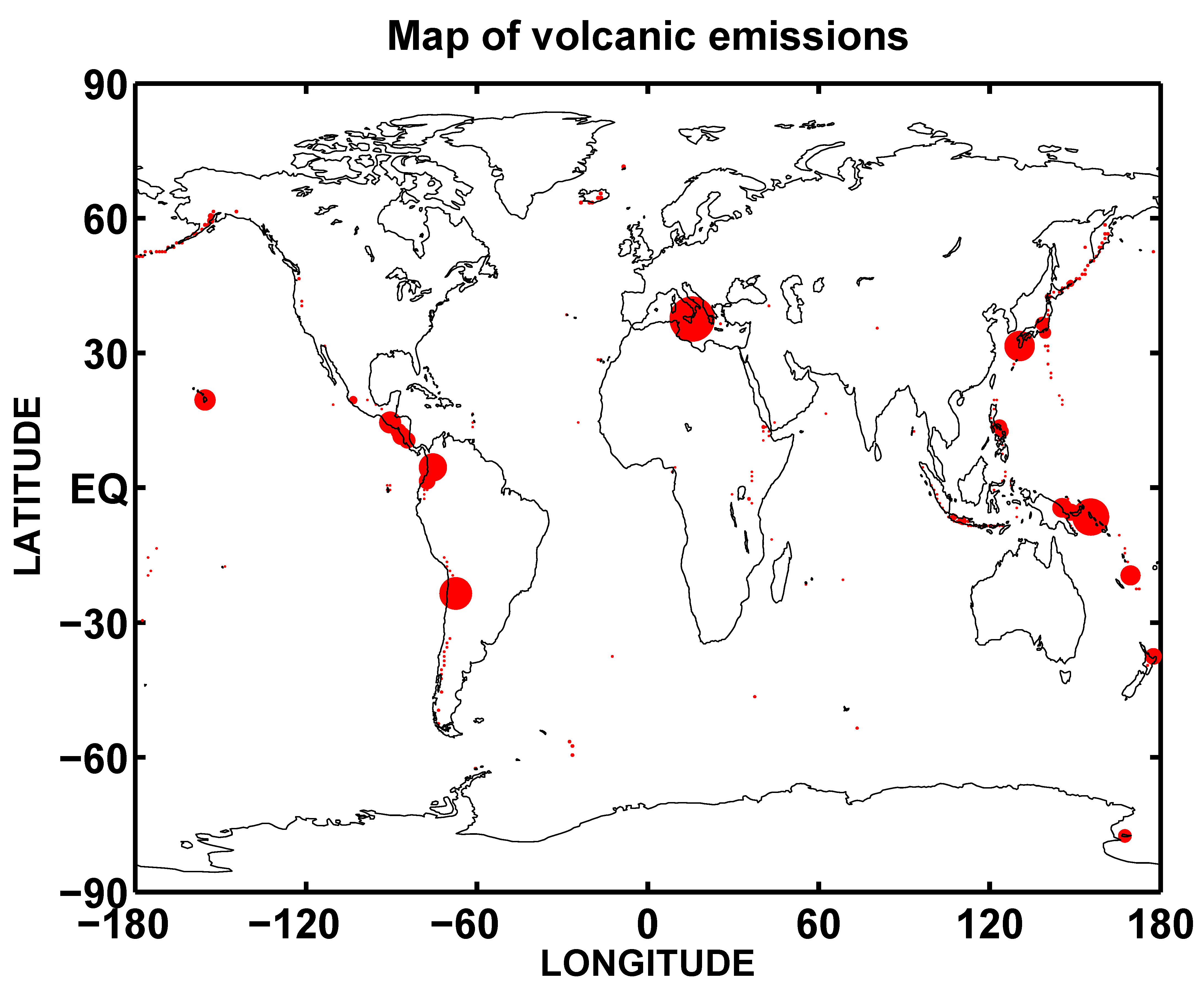
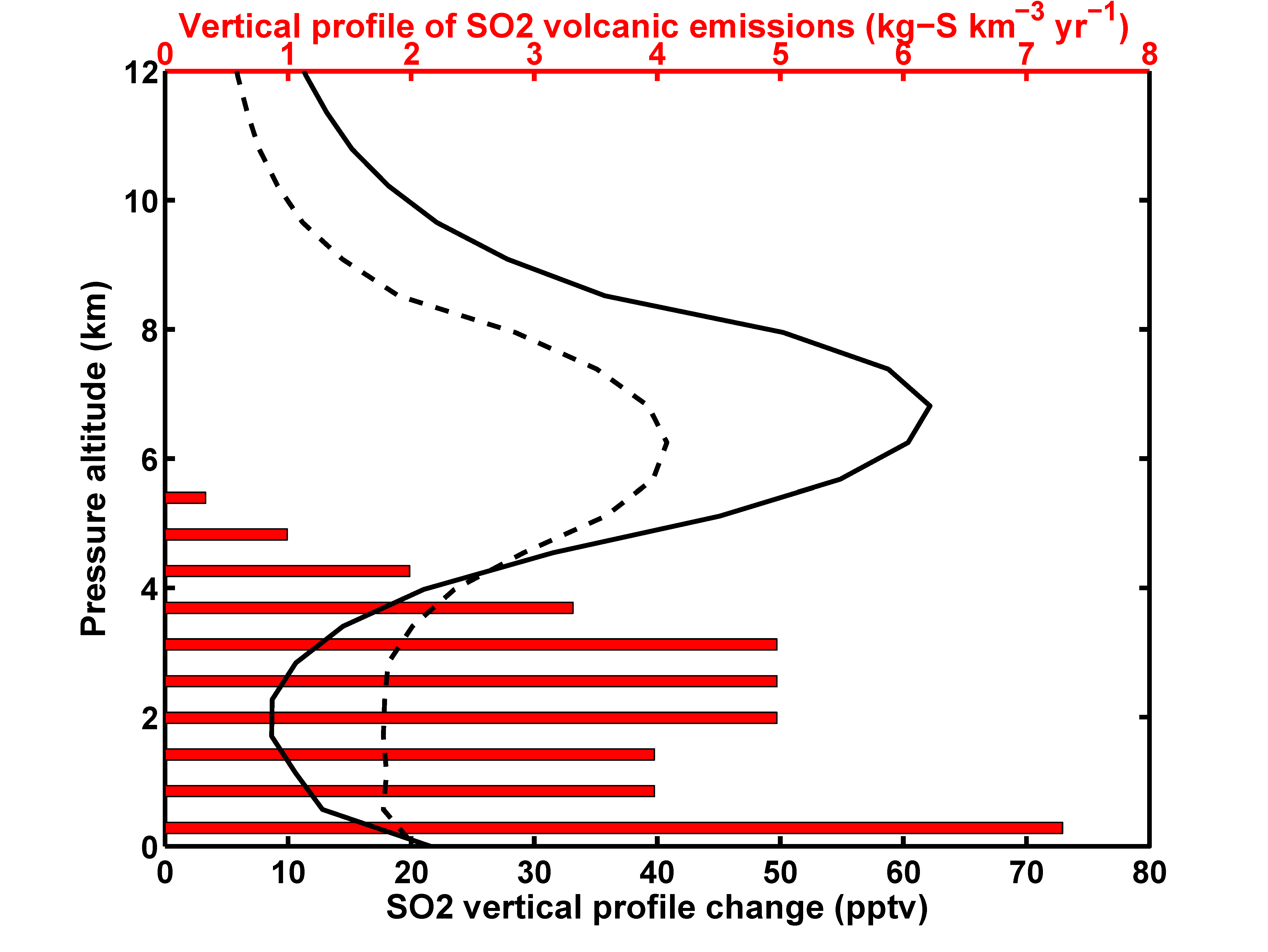
2.2. Numerical Experiment Setup and Sulfur Budget

In order to study volcanic emission effects on aerosol extinction, optical depth, surface area density, UT ice particles, SO4, NOx, O3 mixing ratios and O3 column, two different scenarios have been prepared, one including non-explosive volcanic emissions and the other excluding them. Volcanic SO2 emissions are taken from Penner et al. [2], with a global amount of 9.6 Tg-S/yr and a fixed vertical distribution, as discussed in the introduction section (see also the model formulation summary in Appendix).
The model has been run for two time-slice simulations of 20 years each, with year 2000 atmospheric chemistry conditions, as specified in the SPARC-CCMI modeling exercise [17] for surface mixing ratios of long-lived species and surface fluxes of NOx, CO, VOC SO2 and tropospheric aerosols. Observed sea surface temperatures (SSTs) from 1991 to 2010 are used in the simulations to produce a realistic interannual variability. The “reference” simulation (REF) does not include the volcanic aerosols, which are included, on the other hand, in the “volcanic emission” case (VE). Aerosol-chemistry-radiative perturbations are calculated as VE-REF using an average over the last 15 years of each simulation (1996–2010).
An assumption has been made in our experiment, in order to isolate the chemical-radiative effects of aerosols in the calculation of VE-REF anomalies of the chemical species. Changes in temperature and wind fields due to the volcanic aerosols would in fact mask their direct chemical-radiative effects on tracer species and for this reason the VE case has been run with the same temperature and winds as the REF simulation in the chemistry-transport module. In other words, the experiments have been designed in such a way as to retain only the volcanic aerosols direct effects on species photolysis and surface area density in the chemistry-transport module. This is particularly important for the rather small VE-REF ozone anomalies in the lower stratosphere. It should be considered, however, that accounting for additional feedbacks (i.e., temperature and winds) may affect the magnitude of these perturbations. On the other hand, aerosols from non-explosive volcanoes are largely located in the troposphere and do not produce any stratospheric warming and westerly wind anomaly, contrary to aerosols from major volcanic eruptions which may significantly affect the stratospheric Brewer-Dobson circulation [12].
Climate and dynamical changes, however, are obviously considered for the prediction of UT cirrus ice particles. Following the parameterization described in Kärcher and Lohmann [22], ice particle number density and size are primarily controlled by temperature and by the updraft velocity magnitude, which in turn regulates the adiabatically raising amount of water vapor that may eventually produce ice supersaturation conditions for homogeneous freezing. These dynamical variables may obviously be significantly affected by climate perturbations induced by the volcanic aerosols. In order to avoid an obvious bias in the model prediction of VE-REF climate changes, an approximated simple approach is used for SSTs in the REF simulation. In this no-volcano case, SSTs are specified using the same observed values as for the VE case [33], but decreased with a uniform globally averaged value ΔT = 0.07 K, calculated as ΔT = 0.3 × RF [34], where RF is the globally averaged radiative flux change at the tropopause due to the non-explosive volcanoes (see ahead Section 3.5).
The sulfur budget in the ULAQ-CCM is summarized in Table 1: SO2 and SO42− calculated lifetimes are 2.1 and 5.7 days, respectively. These values are consistent with independent estimates [7,14,35]. The sulfate lifetime (almost entirely determined by SO42− wet deposition) is in the range of values reported in Penner et al. [2] (4.9 ± 1.0 days) and ~15% longer than the mean value. On the other hand, it is less than half the value indirectly estimated for tropospheric aerosols in a recent study by Kristiansen et al. [3], obtained by diagnosing the e-folding time of surface deposited Cesium 137 from the March 2011 major nuclear accident of Fukushima, Japan (14.3 ± 1.3 days from station measurement data between 2 and 9 weeks after the start of the emission). The calculated SO2 lifetime is also in the range of values reported in Penner et al. [2] (1.8 ± 1.0 days), as well as SO2 and SO42− burdens (0.46 ± 0.14 and 0.77 ± 0.19 Tg-S, respectively). Table 1 also shows the efficiency of sources in sulfate production (defined as the fractional contribution to the sulfate burden divided by the fractional source strength). The ULAQ-CCM calculated efficiency for non-explosive volcanoes is 1.64, which is a factor 1.8 larger than the efficiency calculated for the other sources. Qualitatively similar results were found in Graf et al. [14]; however, the efficiency was even larger than in our case (2.63) and a factor of 3 larger than for the other sources. The main reason for this difference should be found in their choice of a larger SO2 dry deposition on land (0.6 cm/s) [36], with respect to 0.1 cm/s as in our case [37], which implies a significant longer lifetime for anthropogenic SO2. The sulfur efficiency was recalculated by Feichter et al. [38], with this update for the SO2 dry deposition velocity. They found a decrease by a factor 2.3 of the ratio between volcanic and anthropogenic efficiency. The dry deposition irreversible sink of SO2 near the surface is indeed the direct justification for the larger efficiency of volcanic sulfur, due to the significant fraction of their emission taking place above the boundary layer.
The latitudinal distribution of sulfur emissions from non-explosive volcanoes is shown in Figure 1, with superimposed the model calculated aerosol optical depth (AOD) from this volcanic source (λ = 0.55 µm). The calculated globally-annually averaged AOD is 5.3 × 10⁻³, that is 14% of the REF value (i.e., the AOD from all other sulfur sources: anthropogenic, biomass burning, oceanic and OCS photolysis) and 12% of the total VE AOD. The calculated zonal mean AOD closely follows the emissions, due to the rather short lifetime of tropospheric sulfate. Volcanic emissions are largely localized in the tropics and subtropics, with the greatest contribution from the so-called “Pacific ring of fire” (see Appendix).
One of the key points in the present study is to assess the link between the tropospheric source of volcanic sulfur and its effects in the lower stratosphere, through heterogeneous chemical reactions and perturbation of photolysis rates. For this reason, we present in Table 2 the stratospheric sulfur budget, with calculated lifetimes of 30 days for SO2 and 1.0 year for SO42−. These lifetimes are consistent with the e-folding time of stratospheric SO2 and SO42− after explosive eruptions, from both measurements [11] and model calculations [12,39]. The SO2 stratospheric source is set equal at the steady state to the OH loss rate integrated above the thermal tropopause (0.145 Tg-S/yr), with non-explosive volcanoes representing a 5.0% contribution to it (0.007 Tg-S/yr), via SO2 deep convection and large-scale vertical ascent up to the tropical tropopause layer (TTL) [40] (see Appendix). The stratospheric SO42− source is set equal at the steady state to the sulfate loss calculated as the net downward flux at the thermal tropopause, due to large-scale transport and gravitational sedimentation of aerosol particles. According to the ULAQ-CCM, ~90% of this source is from SO2 oxidation by OH and the remaining 10% comes from tropospheric sulfate aerosols transported at the TTL. A stratospheric sulfate source of 0.010 Tg-S/yr comes from TTL sulfur of volcanic origin, 0.007 Tg-S/yr of which are from TTL transported SO2 and the remaining 0.003 Tg-S/yr from TTL transported sulfate.
The model calculated annual mean SO2 mixing ratios at the TTL are 27 and 29.5 pptv for REF and VE simulations, respectively, with a standard deviation σ = 5 pptv calculated as the average value of the monthly mean dispersion over the 15 years considered in the simulation time average. These are consistent with the value of 25 ± 10 pptv obtained from MIPAS measurements taken from 2002 to 2012, excluding the periods affected by volcanic eruptions that had reached the lower stratosphere [41].

3. Results and Discussion

In this section, we will first present the model results in terms of aerosol products along with their evaluation using satellite data, then the volcanic aerosol impact on UT cirrus ice particles, on tropospheric and stratospheric chemistry and finally on tropopause radiative fluxes (with direct and indirect effects). Satellite and aircraft data will be used to evaluate the model calculated aerosol products, tropospheric NOx profiles, UTLS O3 distribution and ozone column.

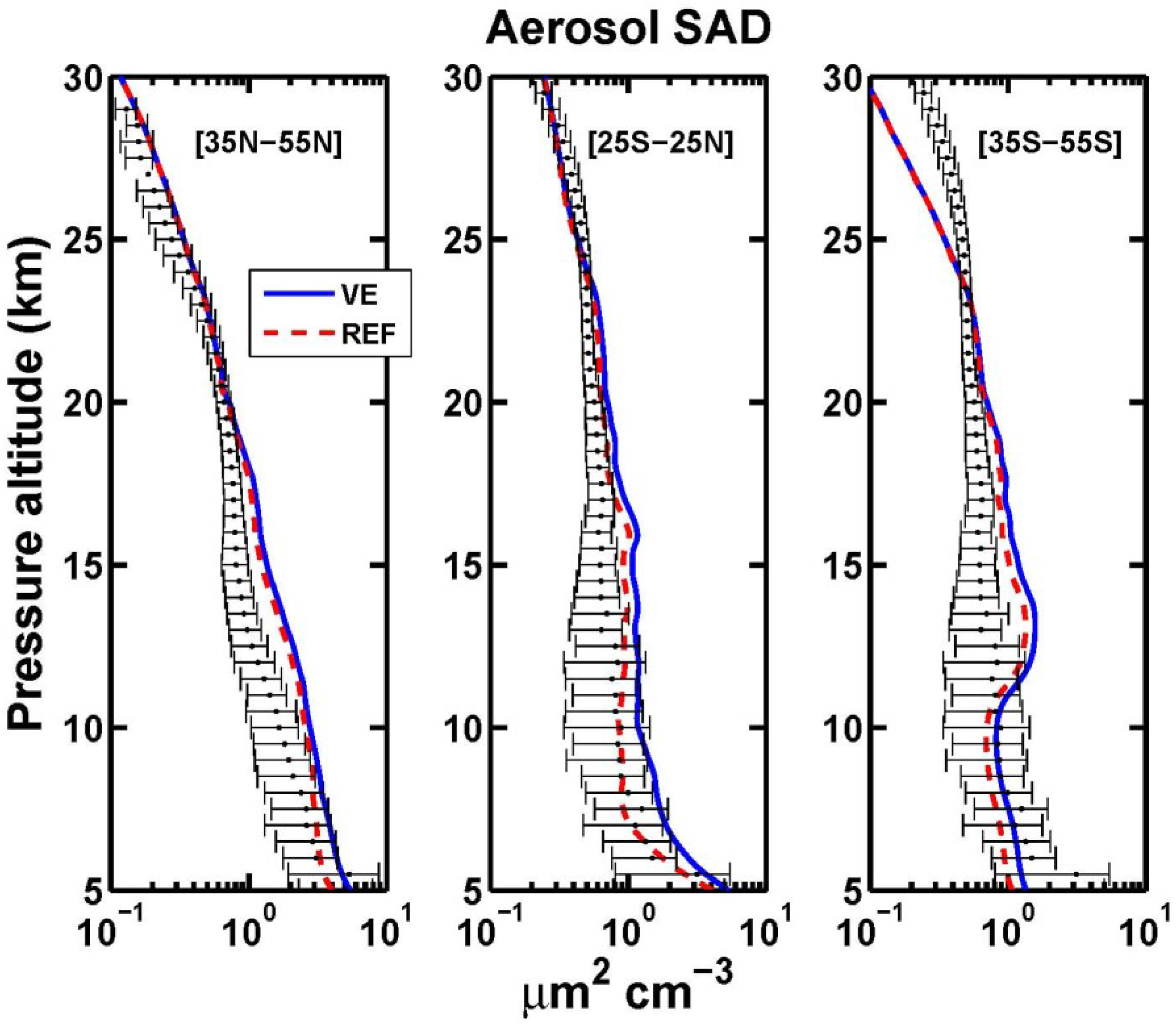
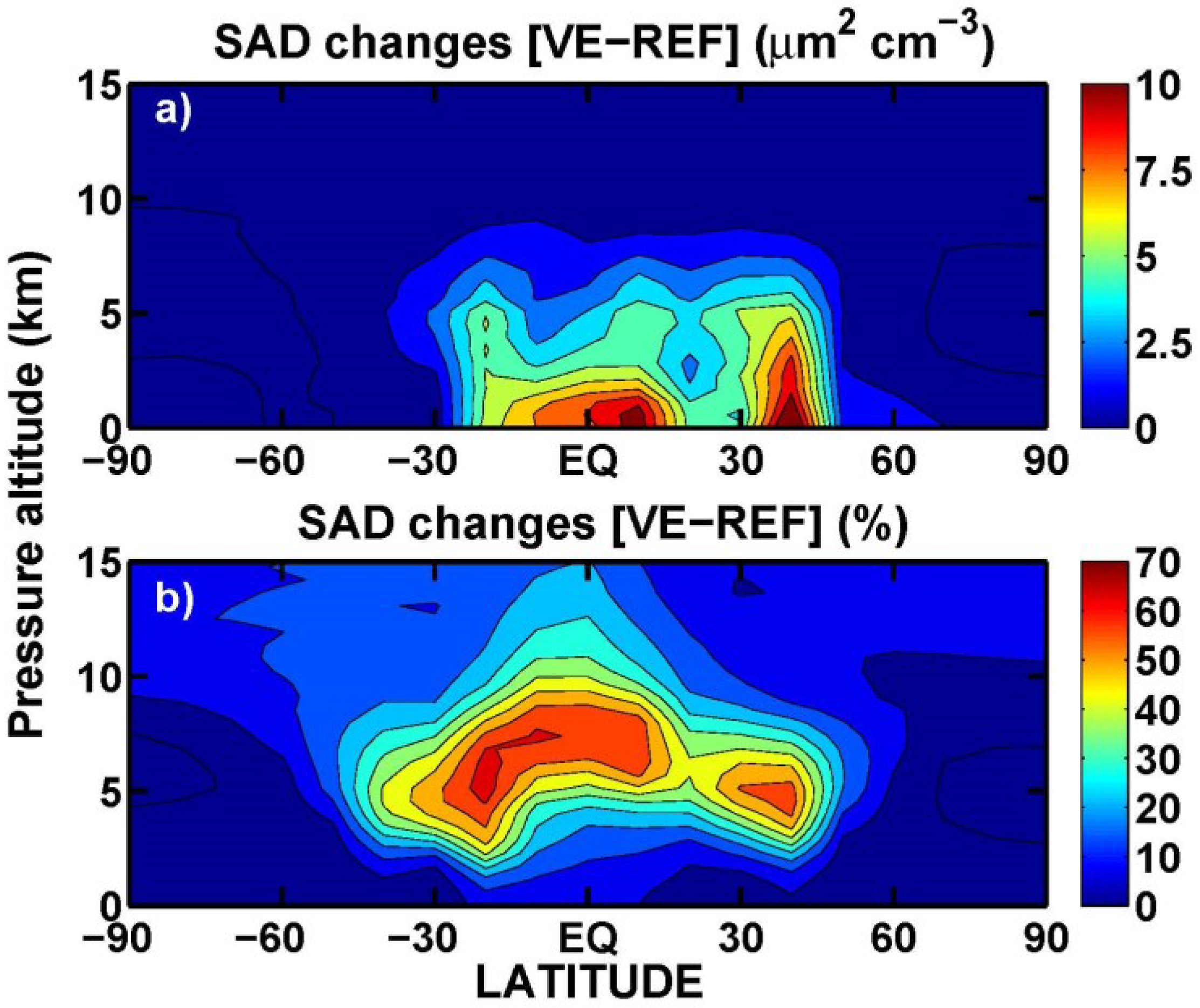
3.1. Aerosol Products

The vertical profiles of aerosol extinction calculated using the size distribution of the various aerosol families in the ULAQ-CCM (i.e., sulfate, organic and black carbon, nitrates, soil dust and sea salt) are shown in Figure 2 and compared with SAGE-II data [39], averaged over 1999–2002. Except for some overestimation at the northern mid-latitudes in the UTLS, the ULAQ model is consistent with observations and normally in their uncertainty range. The calculated UTLS AOD (i.e., the extinction vertical integral) is presented in Figure 3a and compared with SAGE-II data, showing again a good agreement and some overestimation at the northern mid-latitudes: the tropical and mid-latitude VE-REF anomaly is in the 10-30% range. The model calculated total AOD (i.e., from the surface to the top of atmosphere) is compared with AVHRR retrievals [42,43] and AERONET data [44] in Figure 3b: the ULAQ-CCM overestimation in the NH subtropics is most likely related to insufficient removal of desert dust aerosols.
A realistic model calculation of the sulfate aerosol surface area density is essential for correctly treating the NOx heterogeneous removal in the troposphere and lower stratosphere, via hydrolysis of N2O5 and BrONO2. In the vertical layer close to UT cold point, the hydrolysis of ClONO2 is also important as a NOx sink, not only on sulfate aerosols, but also on the surface of ice particles. The latter are also considered in the ULAQ model for the N2O5 and BrONO2 reactions in the whole UT, where cirrus ice may form (see ahead). A comparison of the model calculated surface area density (SAD) for all the aerosol particles (which is essentially sulfate SAD in the stratosphere and upper troposphere) is attempted in Figure 4, using SAGE-II derived values. The latter are indirectly obtained from extinction values, so that the contribution of fine particles smaller than the optically active ones in the accumulation mode is not properly captured. For this reason, the comparison in Figure 4 is made with the SAD calculated in the ULAQ model by truncating the size distribution at r = 0.05 µm and ignoring smaller aerosols. The UTLS overestimation in the Northern Hemisphere mid-latitudes is consistent with what was shown in Figure 2 and Figure 3 for extinction and optical depth, respectively, whereas the overestimation in the tropical UT is most likely related to the adopted radial truncation in the model. The latter is in fact the region where homogeneous nucleation is most active in forming H2SO4-H2O molecular clusters and then ultrafine and fine sulfuric acid aerosols, via coagulation and gas condensation [45]. It is thus difficult to operate here a robust comparison with the SAGE-II derived SAD values.
Zonally and annually averaged VE-REF changes of aerosol extinction and SAD are presented in Figure 5 and Figure 6, respectively. The large relative changes of these two quantities in the mid-upper tropical troposphere (~20%–60%) are the direct consequence of the relatively high altitude where a significant fraction of the volcanic emissions is located (~50% above 600 hPa), mostly from the tropical Pacific region. This significantly reduces the volcanic sulfate removal by wet deposition compared to anthropogenic or marine sulfate and greatly increases the volcanic SO2 efficiency in producing SO4, following the definition given in Table 1. This large SAD increase produced by volcanic emissions in the mid-upper troposphere will be found to have a significant impact on tropospheric chemistry (see Section 3.3).

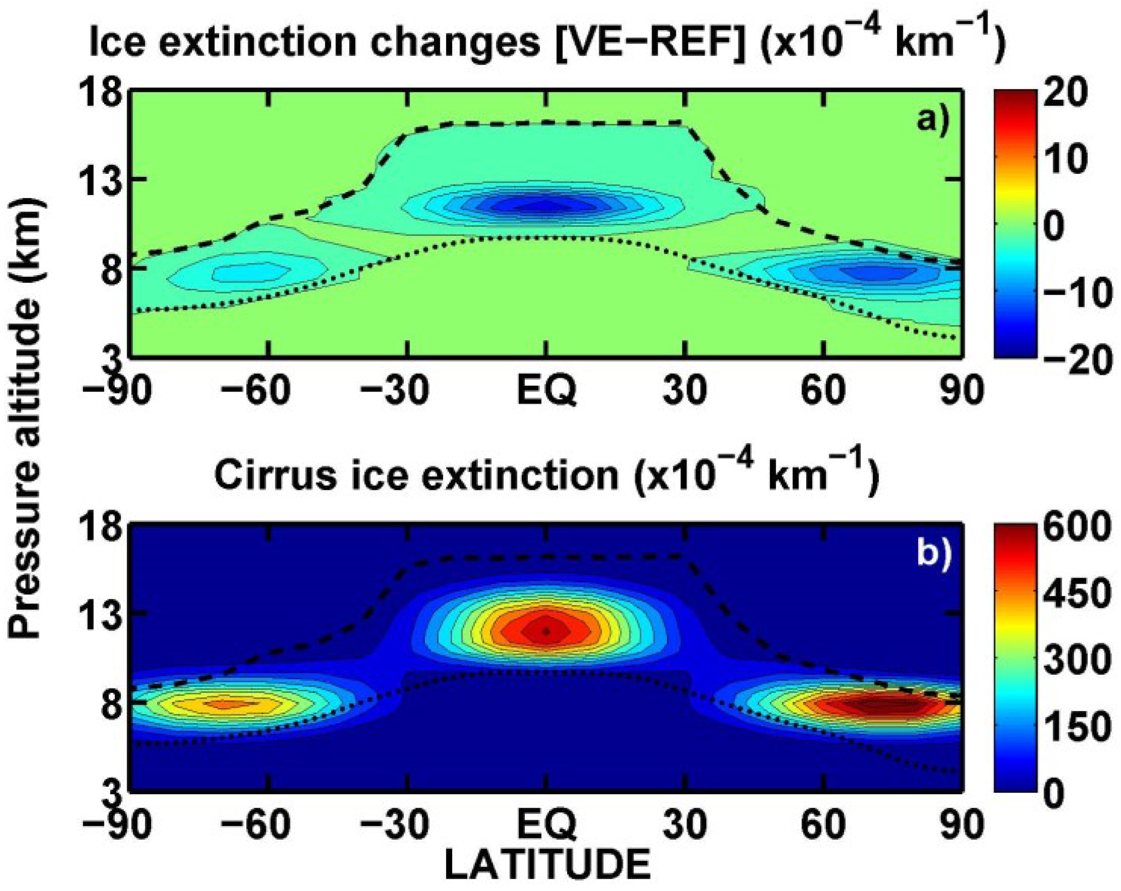
3.2. Upper Tropospheric Cirrus Ice Perturbation

Formation of UT ice particles may take place via heterogeneous and homogeneous freezing mechanisms [46]. Knowledge of the ice supersaturation probability is the starting point for the microphysical model calculations. In the ULAQ-CCM a simple parameterization is adopted, starting from climatological frequencies of relative humidity, from which a mean value and a standard deviation are calculated for the distribution of water vapor mixing ratios. Local ice super-saturation conditions (RHICE > 100%) are a result of turbulent adiabatic ascent [22] and can be found at temperatures below 238 K and below the tropopause. A normal-distribution grid-point probability that RHICE > 100% can be calculated using the water vapor mixing ratio distribution. This represents the probability that an ice particle could be formed via heterogeneous freezing on a preexisting population of ice condensation nuclei (PHET), typically mineral dust transported from the surface or freshly emitted non-hydrophobic aviation BC particles (NICN). The number of ice particles formed via heterogeneous freezing (NHET) is calculated using the ULAQ microphysical scheme for polar stratospheric ice particles formation [47], with NICN used as the population of available condensation nuclei and PHET as the probability that RHICE > 1.1 at any model grid point [46].
UT ice particles may also form by means of homogeneous freezing of supercooled aerosols, which is spontaneous freezing of solution droplets for temperatures below 238 K [48]. This process takes place for higher ice supersaturation ratios, with respect to heterogeneous freezing, typically RHICE > 1.5 [46], for which a probability PHOM can be calculated in the ULAQ-CCM. The number of ice crystals formed through this process (NHOM) mainly depends on temperature and vertical velocity, whereas the aerosol size distribution plays only a minor role [22]. Under normal UT conditions, it dominates ice particle formation with respect to the heterogeneous freezing mechanism. Higher vertical velocities produce higher RHICE and more ice crystals can be formed before the level of supersaturation decreases following water vapor deposition on the ice crystals. On the other hand, lower temperatures lead to more ice crystals because the water vapor deposition is slower and the nucleation rate is faster. The numerical scheme adopted in the ULAQ model is the one developed in Kärcher and Lohmann [22], and this assumes that basic physical processes determine the number of ice crystals (NHOM) formed during an adiabatic ascent, including temperature and updraft speed. The latter is calculated as a function of the turbulent kinetic energy (TKE), following the method outlined in Lohmann and Kärcher [49].
UT ice extinction anomalies VE-REF calculated in the ULAQ-CCM are presented in Figure 7a and are of the order of 3% of the calculated VE values in the tropical layer at 10–12 km altitude (Figure 7b). The anomalies are negative in the whole UT, as a result of the surface cooling produced by the volcanic aerosol additional radiation scattering. This result is qualitatively consistent with the findings of Kuebbeler et al. [23] for geoengineering sulfate aerosols. They note that the eruption of Mt. Pinatubo cooled the Earth’s surface globally by ΔT ~0.5 K. The surface cooling produced by geoengineering or major explosive eruptions modifies the tropospheric vertical temperature distribution, also for the tropical stratospheric warming [12]. This induces a stabilization of the troposphere and reduces the vertical velocity associated to TKE. The simulations of Kuebbeler et al. [23] suggest that the reduced vertical velocity directly influence the rate of homogeneously formed ice crystals. The ULAQ-CCM simulations also show a reduction in the formation of ice crystals in the 10–12 km altitude layer over the tropics, due to the simultaneous decrease of vertical velocities and temperature. The UT cooling effect tends to offset the reduction in updraft above 12 km altitude up to the tropical tropopause, with a slight increase in the concentration of ice particles. However, the model also shows a decrease of the particle radius above 10 km of altitude up to the tropical tropopause due to the temperature decrease, so that a combination of the model calculated anomalies of ice number concentration and radius produces an ice extinction decrease extended over the whole UT region (Figure 7a) (−0.9% globally).
An evaluation of the model calculated number concentration (Ni) of UT ice particles is difficult, because one of the critical parameters at the time of ice formation (i.e., updraft vertical velocity producing ice supersaturation) is usually not known. In addition, very few in situ measurements are available for ice clouds formed in rising air parcels with relatively slow vertical velocities (10–20 cm·s−1), which are typical values obtained in a large-scale model as a function of TKE. However, as noted in Kärcher and Lohmann [22], their scheme for ice crystals formation via homogeneous freezing is in general very good agreement with airborne measurements of Ström et al. [50]: they reported Ni = 0.3 cm−3 in a young cirrus cloud at T = 220 K, with w~0 on average and ~20 cm·s−1 as a standard deviation. The Kärcher and Lohmann [22] scheme predicts Ni = 0.18 cm−3 with w = 10 cm/s and Ni = 0.5 cm−3 with w = 20 cm·s−1 at T = 220 K. The ULAQ-CCM predicts a climatological average value of NHOM = 0.02 cm−3, with w = 22 ± 2 cm·s−1 and an average probability PHOM = 4% (at T = 220 K, p = 200 hPa in the tropical region). It should be noted that this PHOM is consistent with the distribution of vertical velocities in the ULAQ-CCM, considering that the values recorded by Ström et al. [50] (i.e., w = 0 ± 20 cm·s−1) imply a probability of ~4.4% for a w range of 20–24 cm/s (i.e., the ±1σ interval in the ULAQ-CCM).
Due to the typical size of these ice particles (r~20 µm), the extinction values (πr2QextNHOM) are close to half of the particle SAD, because Qext~2. The UT tropical ice SAD is then typically in the range of 50–100 µm2·cm−3, which is almost two orders of magnitude larger than the sulfate aerosol SAD in the same region. The efficiency of the heterogeneous NOx sink on ice is then significantly larger than on sulfate, even though the reaction probability of N2O5 on ice is approximately a factor of 5 smaller than on sulfate. In addition, the hydrolysis of N2O5 may reach saturation in presence of high SAD values [51].

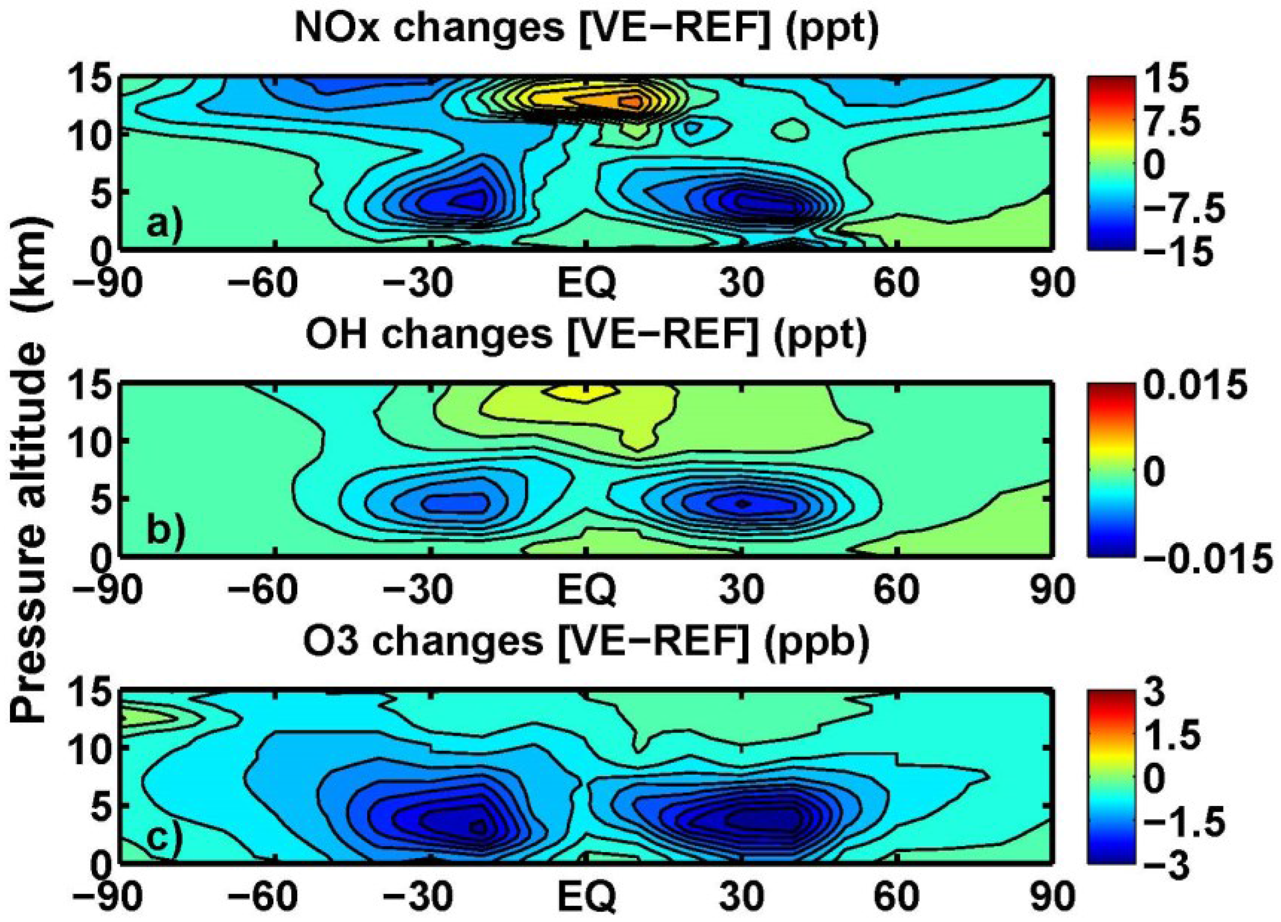
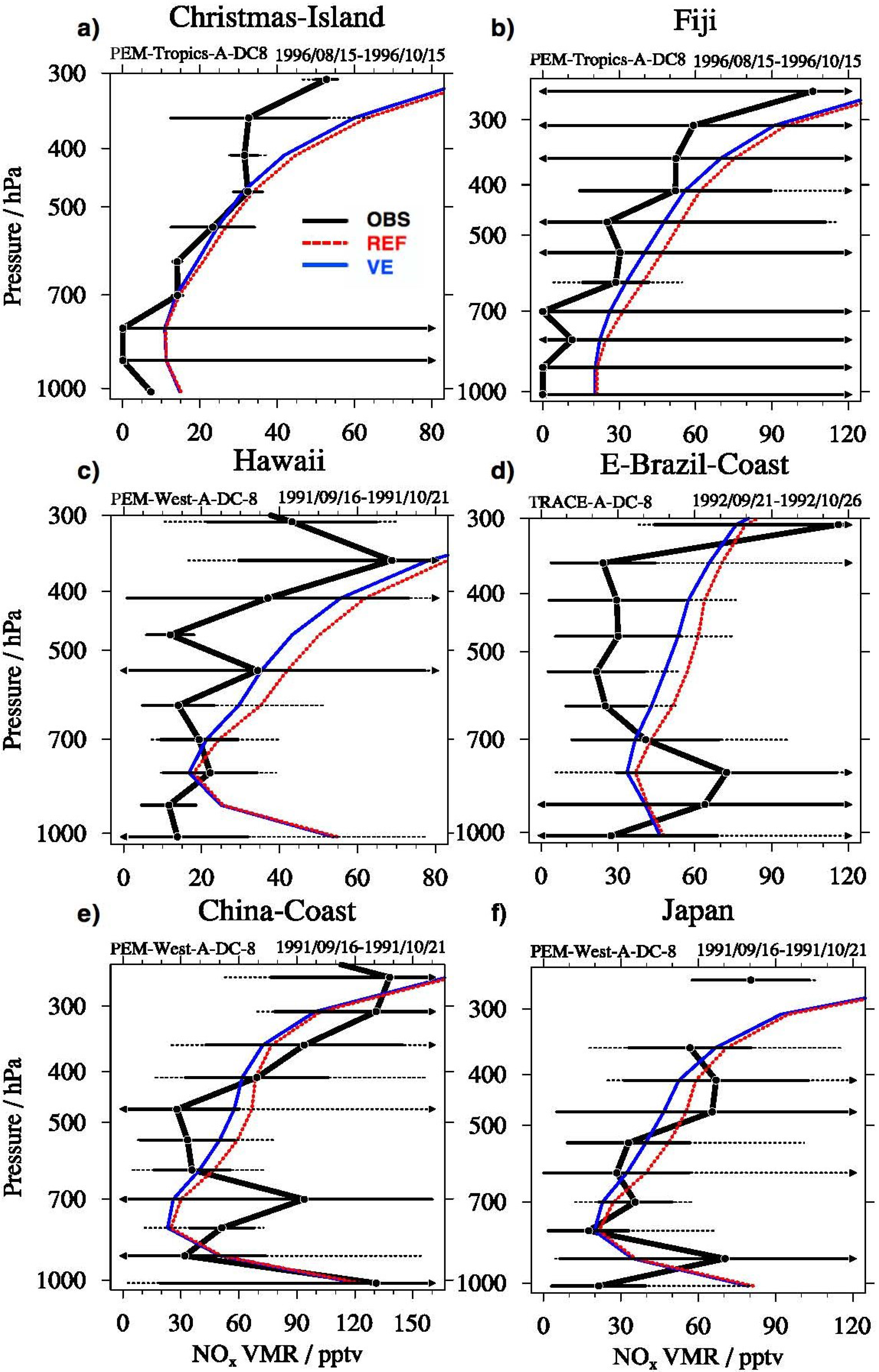
3.3. Tropospheric Chemistry Perturbation

The impact of volcanic aerosols on tropospheric chemistry is mainly produced by the enhancement of sulfate SAD available for heterogeneous chemical reactions that act as a NOx sink (i.e., hydrolysis of N2O5 and bromine, chlorine nitrates). This type of removal contributes to the net NOx loss term along with NO2 reactions with OH (forming HNO3) and organic radicals (forming PAN and organic nitrate aerosols). It is then important to consider also the NOx partition into NO and NO2, which is regulated by the abundance of O3 and the photolysis of NO2. The consequent NOx depletion is evident in Figure 8a: it follows the relative changes of sulfate SAD, coupled to the fact in proximity to the equator the dominant NOx mechanisms for production and loss are convection and lightning, on one side (production), and depletion by OH, on the other side (loss). The tropical UT increase, on the other hand, is produced by the reduced impact of the sulfate SAD enhancement in presence of a large background ice SAD, which in turn decreases (as shown in Figure 7a); and by the simultaneous increase of NO2 photolysis due to the additional radiation scattering by the volcanic aerosols (see Section 3.4). A decreased amount of NO2 in favor of NO makes the NOx to HNO3 conversion less effective. The OH perturbation (Figure 8b) is directly linked to that of NOx and is important for tropospheric chemistry because it regulates the CH4 lifetime [52,53] and its longwave forcing in the global radiative budget (see Section 3.5). The O3 perturbation (Figure 8c) is also regulated by that of NOx, because the tropospheric O3 production is regulated by NO reactions with HO2 and organic radicals RO2 (mainly CH3O2). The most important O3 removals are dry deposition in the boundary layer and reactions with HOx in the free troposphere (with decreasing OH and increasing HO2). Tropospheric O3 changes may also be non-negligible for the global radiative budget.
A sample evaluation of model results for tropospheric NOx is made in Figure 9, using data from a collection of aircraft campaigns [54]. Solid blue and dashed red lines show model profiles (VE and REF, respectively) at the same latitude and longitude of the campaign, including the uncertainty interval of the observations (±1σ). In general, the modeled vertical profiles conform to the range of variability of the measurement data, with VE profiles highlighting a ~20% reduction of the REF mixing ratios in the mid-tropospheric subtropics and northern mid-latitudes (see also Figure 8a). The range of uncertainty in the measurements is too large for drawing conclusions on the relevance of the NOx depleting effect due to the volcanic aerosol SAD.
An evaluation of the model calculated O3 mixing ratios in the troposphere and lower stratosphere is presented in Figure 10, using HALOE and TES/Aura satellite data. The large latitudinal gradient of the O3 mixing ratio is well captured by the ULAQ model. It is worth noting that the O3 retrieval from TES/Aura radiances in the UTLS features a tendency to overestimate the chemical tracer with respect to HALOE observations. The O3 column is compared to NIWA combined total column ozone data [55] in Figure 11, where we also show the calculated O3 column changes (VE-REF). The negative column ozone changes from 40S to 40N are in the range −0.5 DU to −1.0 DU; these are largely due to the mid-tropospheric negative values shown in Figure 8c and produced by the NOx depletion caused by the volcanic aerosols. The NOx depletion in the lower stratosphere also plays a significant role (see Section 3.4). The annual mean zonally averaged total column is in very good agreement with NIWA data, except for a model underestimation in the Southern Hemisphere sub-polar region.

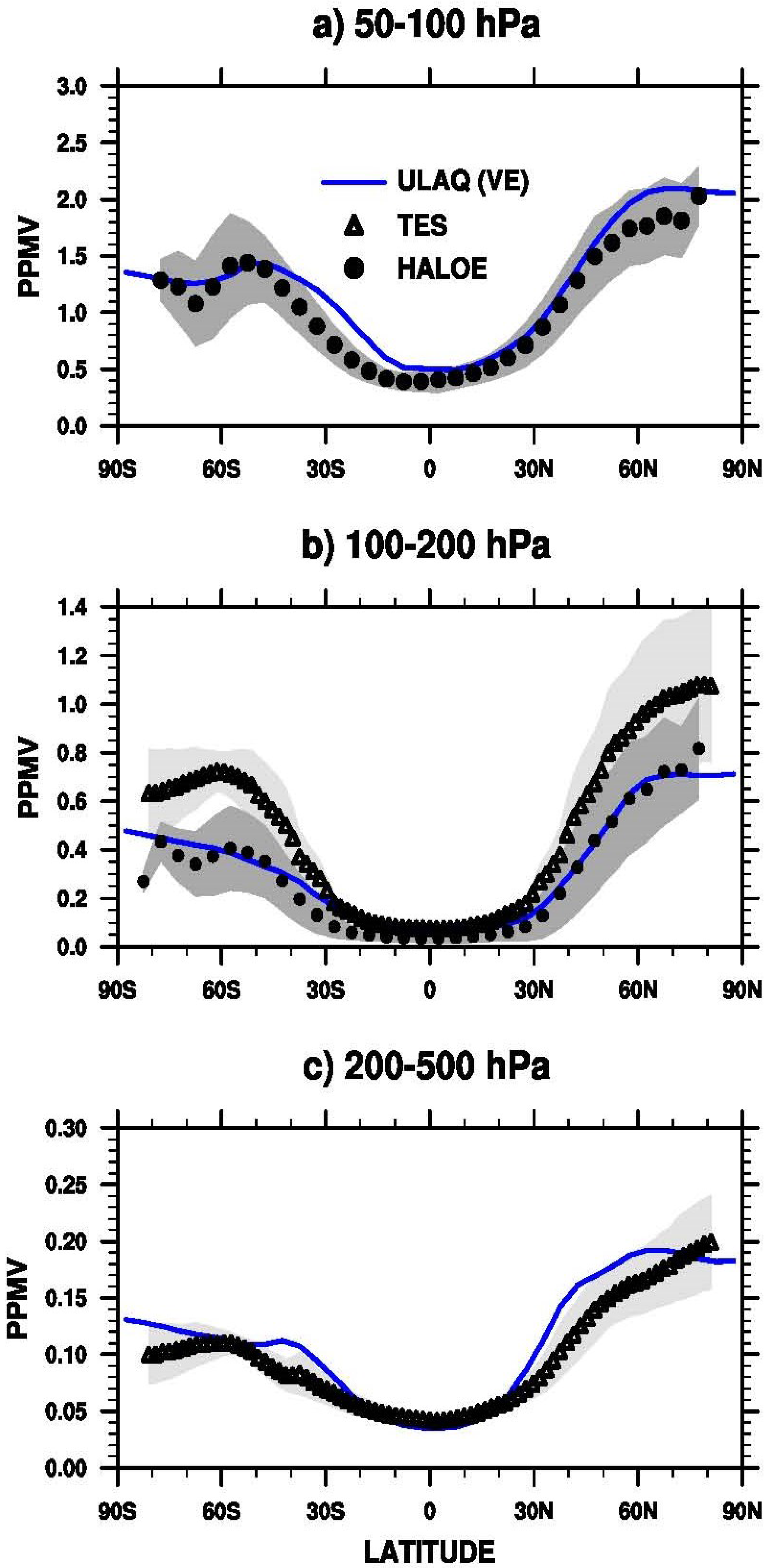
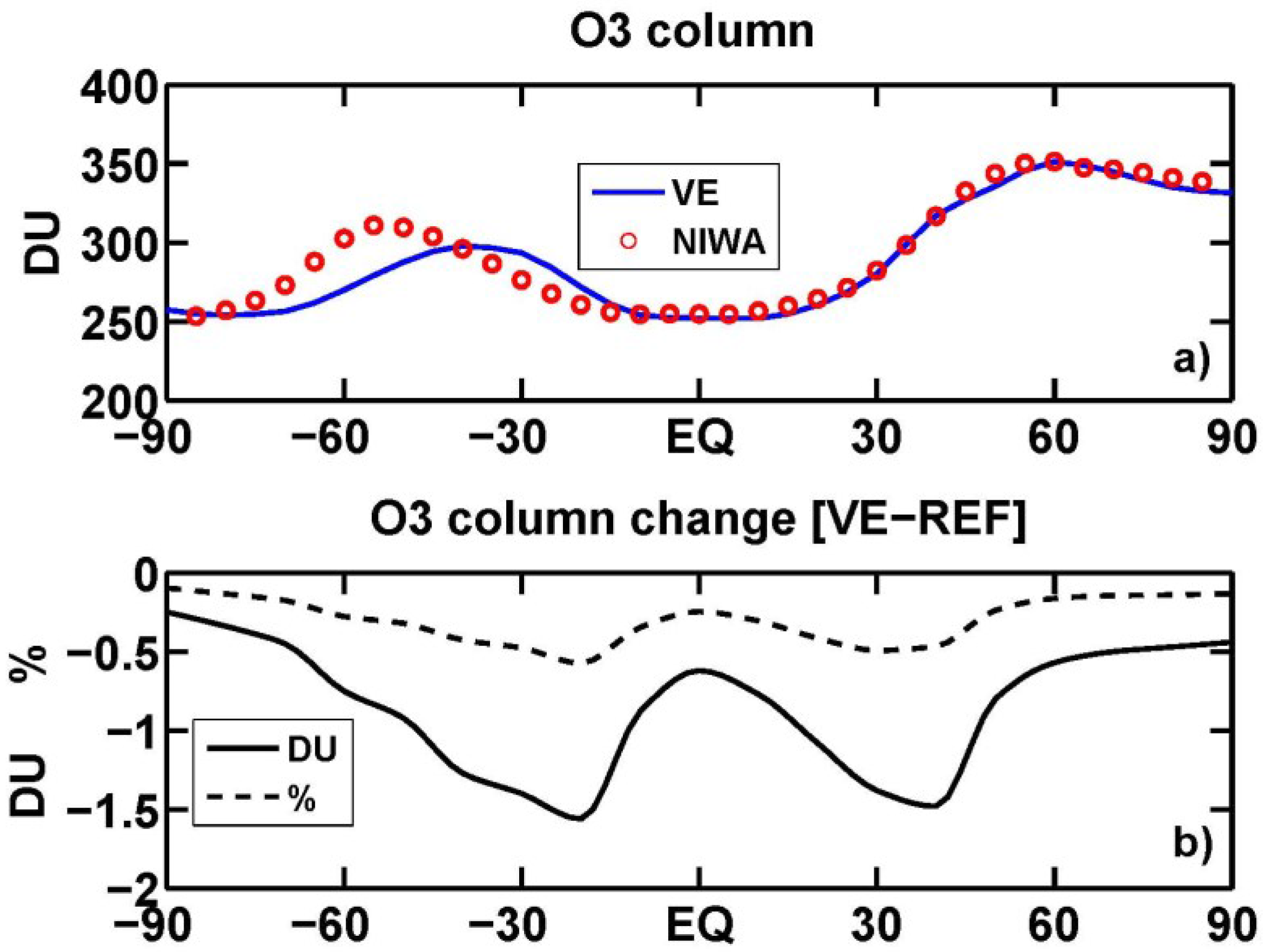
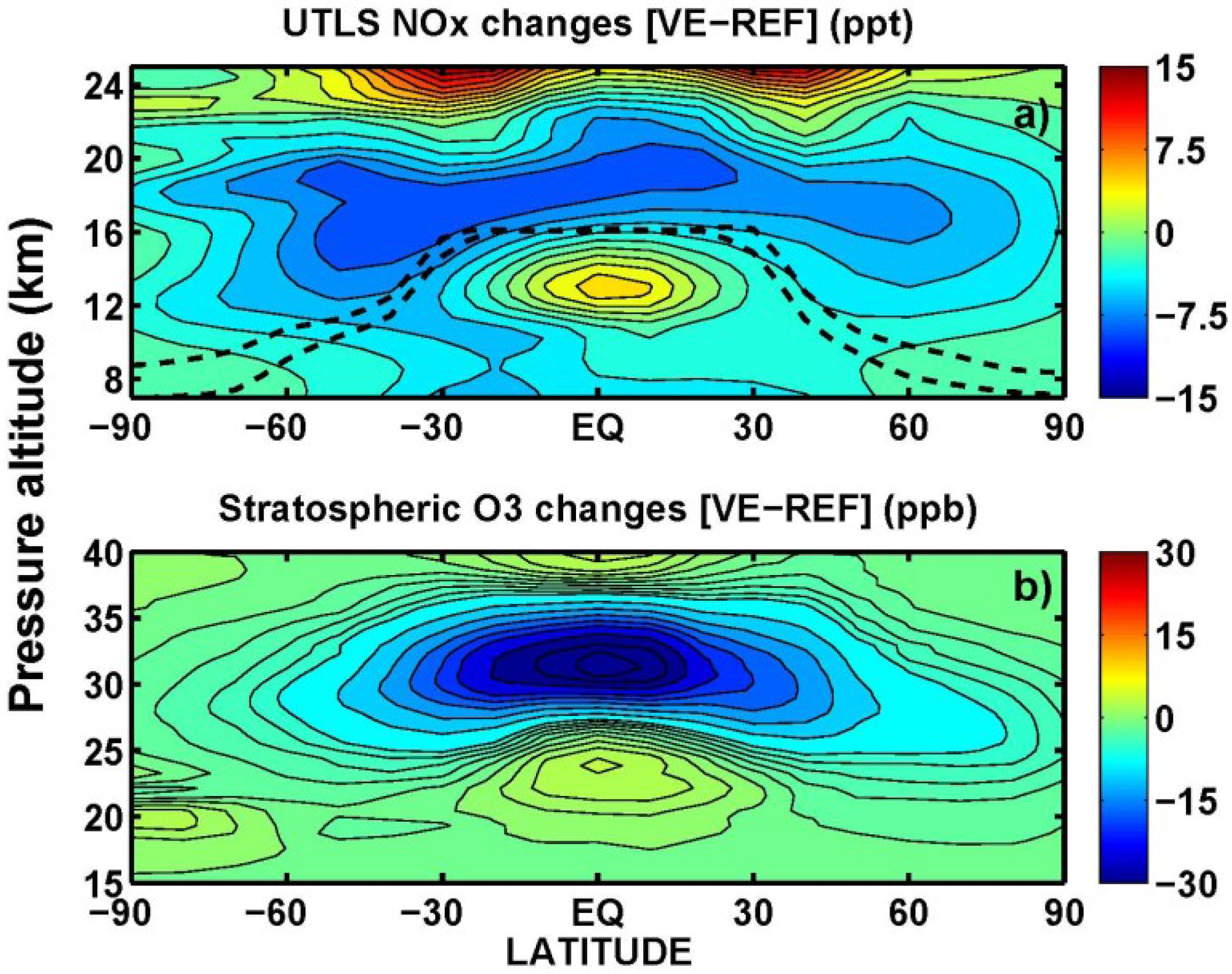
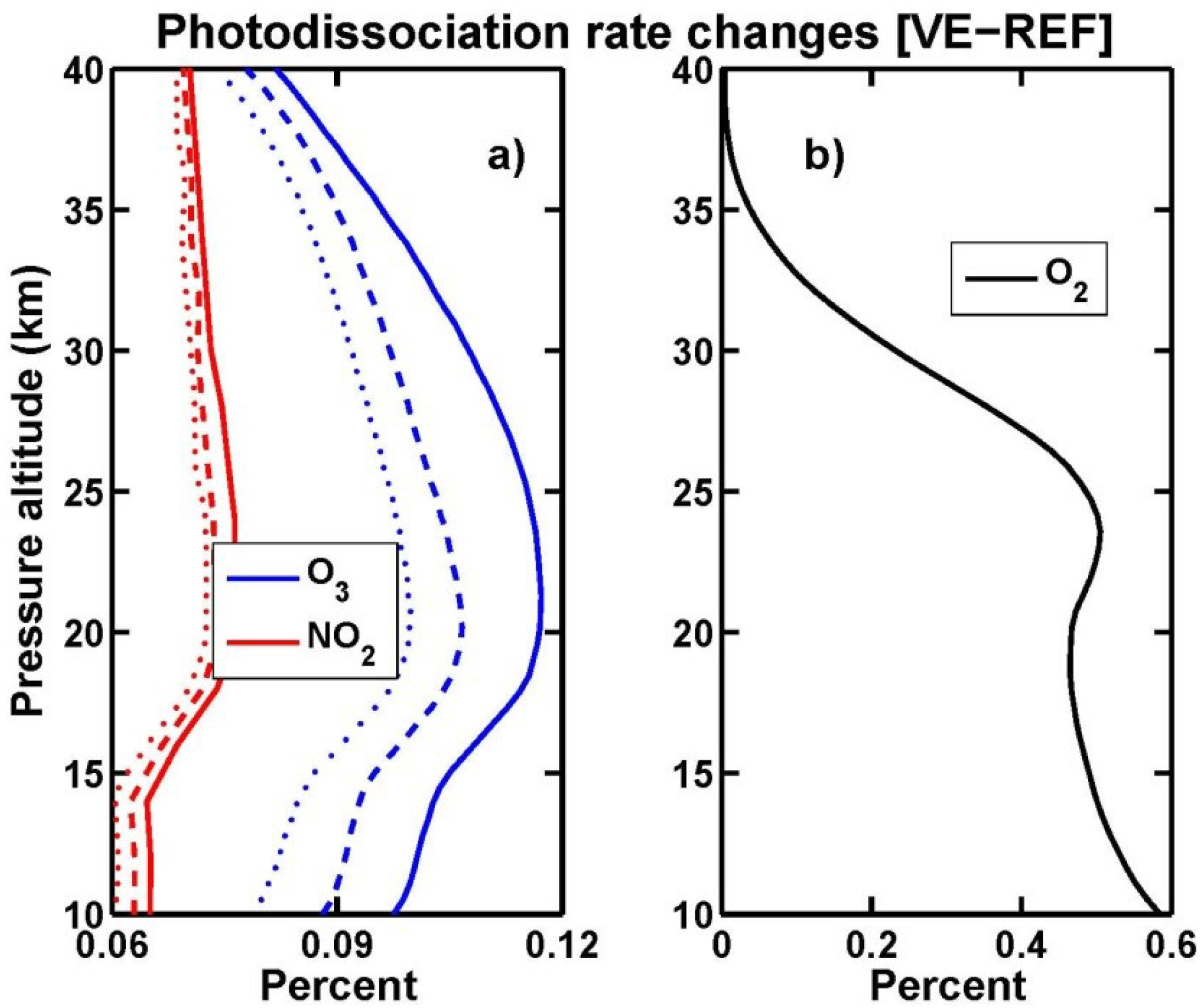
3.4. Stratospheric Chemistry Perturbation

Tropospheric SO2 in the tropical region can be efficiently transported vertically up to the TTL (see Table 2), via deep convection from the boundary layer and large-scale vertical ascent [40]. This represents one of the main sources for stratospheric sulfate, along with photolysis of OCS [39,47,58]; the role of OCS as a source for stratospheric sulfate has been recently re-examined in Sheng et al. [59].
If we look at sulfate changes produced by the volcanic aerosols in the UTLS (Figure 12a), we obtain a clear “secondary maximum” of the SO4 anomaly immediately above the tropopause from pole to pole, following this SO2 fast transport to the TTL, subsequent OH oxidation and sulfate formation and finally isentropic large-scale transport towards mid-high latitudes. Here the SO4 lifetime is much longer than in the troposphere and most of all with respect to the tropical UT, where efficient sulfate loss may take place via ice sedimentation. An average of the sulfate SAD changes above the tropopause and up to 25 km altitude is presented in Figure 12b, with relative changes peaking up at 10%–15% in the Southern Hemisphere. Here the REF SAD is on average smaller than in the Northern Hemisphere, where much larger values of tropospheric SO2 come from anthropogenic emissions. The impact of sulfate and ice SAD changes on the total heterogeneous loss frequency of NOx (i.e., hydrolysis of N2O5, BrONO2, ClONO2) is presented in Figure 12c. Above the tropopause, the relative changes of the NOx heterogeneous loss frequency are well correlated with the SAD relative changes shown in Figure 12b. Much smaller or even negative changes are found in the upper troposphere, due to the large background ice SAD and its negative VE-REF changes (Figure 7) (although the latter are rather small in percentage of the background magnitude, when compared to the sulfate SAD relative changes seen in Figure 6b).
Sulfuric acid aerosol SAD affects primarily NOx in the lower stratosphere and also the abundance of chlorine/bromine radical species, following the decrease of Cl/Br nitrates associated to the enhanced NOx conversion into nitric acid. The VE-REF NOx anomaly in the UTLS is presented in Figure 13a and (as expected) is consistent with the increase of the NOx heterogeneous loss frequency changes seen in Figure 12c. A mid-stratospheric NOx increase is also calculated (~10–30 pptv in the vertical layer from approximately 23 to 35 km altitude) and it is due to the volcanic aerosol induced increase of NO2 photolysis, because more UV-A radiation is diffused upward (see Figure 14a). This produces also part of the tropical UT increase of NOx (as discussed in Figure 8). An increase of J-NO2 tends to move the NOx partition more in favor of NO respect to NO2, thus decreasing the efficiency of the main gas phase NOx removal mechanism, i.e., NO2 + OH ₒ HNO3. The same photolysis effect is produced on J-O3 (see Figure 14a): this positive change, coupled with the increased NOx amount, induces the mid-stratospheric O3 decrease presented in Figure 13b (~10–30 ppbv in the vertical layer from approximately 25 to 35 km altitude). The slight O3 increase in the tropical lower stratosphere (~18–25 km) comes from the so-called self-healing effect: UV radiation is enhanced in the layer below the region of O3 decrease, promoting an increase of O2 photolysis (Figure 14b) and then producing additional O3 [60,61].

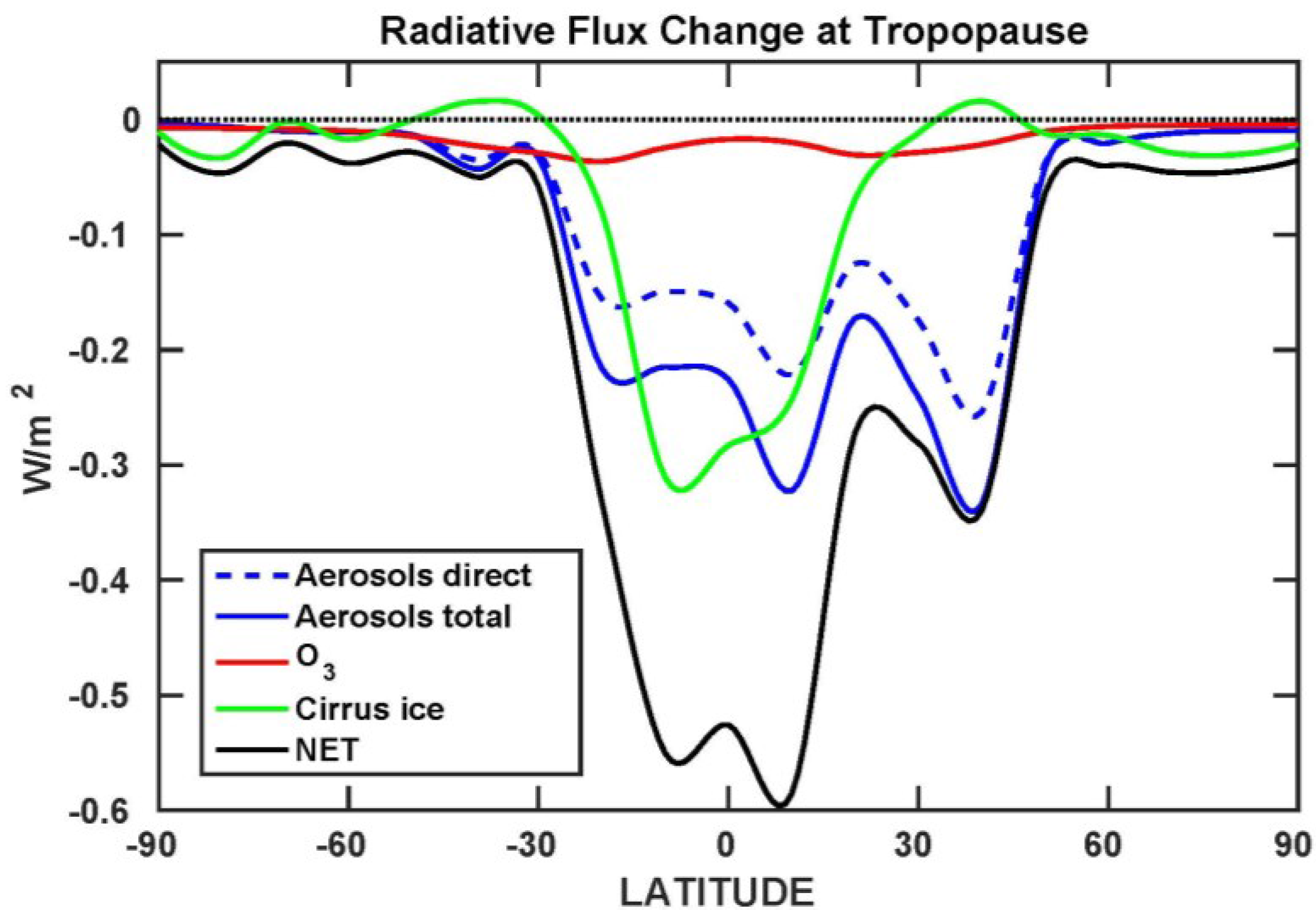
3.5. Tropopause Radiative Flux Changes

The ULAQ Radiative Transfer Module (ULAQ-RTM) was used to calculate the radiative flux changes at the tropopause, related to VE-REF differences for both gases and aerosols. The ULAQ-RTM uses a Mie scattering program to process aerosol optical properties from the OPAC database and size distributions from the ULAQ-CCM to compute the relevant wavelength-dependent aerosol optical properties (extinction, absorption and asymmetry parameter at all vertical layers of the model) [30,32]. All-sky cloud coverage is computed using a maximum-random overlapping scheme from MODIS Terra and Aqua Level 3 data, while surface albedo is derived from MERRA 2D data.
An overall synthesis of the radiative calculations is presented in Table 3, with globally and annually averaged direct and indirect tropopause radiative flux changes (VE-REF). The calculated column ozone change above the thermal tropopause accounts for 23% of the total (ΔO3 strat = −0.23 DU; ΔO3 trop = −0.77 DU). Globally, the CH4 positive RF accounts for approximately 50% in magnitude of the negative O3 RF, so that the two chemically-affected greenhouse gases tend to partially cancel each other out. The CH4 RF is calculated using the parametric formula of Myhre et al. [62], which expresses the radiative forcing as a function of the lifetime change (Δτ): CH4-RF(mW·m−2) = χ-CH4(ppbv) × 0.37 × ∆τ/100 × 1.4, where Δτ is the VE-REF change and χ is the average tropospheric mixing ratio (1754 ppbv). An average feedback factor of 1.4 is applied to the tropospheric CH4 mixing ratio to account for the CH4 adjustment to the tropospheric OH perturbation (Prather et al. 2001) [63], since the CH4 model prediction is made using a fixed mixing ratio boundary condition at the surface. Sulfate aerosol and cirrus ice RFs are calculated using the ULAQ-RTM setups described above. The sulfate aerosols indirect forcing on warm clouds is parameterized using scaling factors with respect to the direct RF, as recommended in Fuglestvedt et al. [64].
Model calculated REF values of optical depth (at λ = 0.55 µm), CH4 lifetime and O3 column are: 0.038 and 0.11 for sulfate and cirrus ice optical depths, respectively; 8.9 years for the CH4 lifetime; 283.7 DU for the total O3 column. The calculated global CH4 lifetime is comparable to the value provided in the SPARC multi-model assessment of atmospheric lifetimes, i.e., 8.7 ± 1.4 years [65].
The latitudinal behavior of the different components of RF is presented in Figure 15, considering here only those calculated in the ULAQ-RTM (i.e., all components except CH4, whose globally averaged value is calculated with a parametric formula as a function of the lifetime change). As discussed above, the dominant components are the sulfate aerosol direct and indirect effects and the contribution of the cirrus clouds response to the climate-dynamical perturbations in the troposphere. The latter is comparable to the aerosol RF over the tropics, but is much smaller over the subtropics and mid-latitudes. According to the model, the net RF due to all different components affected by non-explosive volcanic aerosols (except CH4) has a peak in the tropics close to −0.6 Wm−2 and another peak in the Northern Hemisphere mid-latitudes of approximately −0.3 Wm−2.

4. Conclusions

In the present study, we have used a climate-chemistry-aerosol coupled model to study direct and indirect radiative-chemical perturbations produced by sulfate aerosols from non-explosive volcanic emissions, both in the troposphere and lower stratosphere. The ULAQ-CCM has been extensively evaluated in past and on-going modeling inter-comparison campaigns (SPARC-CCMVal, AeroCom, SPARC-Photocomp, and SPARC-CCMI). Several important aerosol interactions have been explicitly considered, namely with solar and planetary radiative transfer, gas species photolysis, heterogeneous chemistry and upper tropospheric ice crystals formation. An evaluation of model results that are relevant for these processes has been attempted using satellite or aircraft campaign data for aerosol products, UT ice, tropospheric NOx, UTLS O3 and ozone column.
Two multi-decadal time-slice runs of a climate-chemistry-aerosol model (using year 2000 atmospheric chemistry conditions) have been designed to study these chemical-radiative effects. A tropopause mean global net RF = −0.23 W·m−2 is calculated (including direct and indirect aerosol effects) with a 14% increase of the global mean sulfate aerosol optical depth and a 0.07%–0.12% increase of NO2 and O3 photolysis rates in the tropical mid-lower stratosphere. A 5–15 pptv NOx decrease is found in the mid-troposphere subtropics and mid-latitudes and also from pole to pole in the lower stratosphere, the latter due to an average 5%–15% increase of the aerosol surface area density above the tropopause up to 25 km altitude. The tropospheric NOx perturbation triggers a column O3 decrease of 0.5–1.5 DU and a 1.1% increase of the CH4 lifetime. The surface cooling induced by solar radiation scattering by the volcanic aerosols induces a tropospheric stabilization with reduced updraft velocities that produce ice supersaturation conditions in the upper troposphere. A global mean 0.9% decrease of the cirrus ice optical depth is calculated with an indirect RF = −0.08 W·m−2.
The overall conclusion of this work is that the atmospheric impact of sulfur emissions from non-explosive volcanoes is significant where the emissions take place (i.e., the tropical mid-lower troposphere, essentially), mainly because of their larger efficiency in producing sulfate with respect to anthropogenic or marine sulfur (which is more abundant, but less efficient). This aspect has been widely covered in previous studies [14]. Here we have also shown how SO2 transport up to the TTL induces chemical changes in the lower stratosphere, with non-negligible effects on NOx and O3. The photolysis rates of these species are also perturbed, as a consequence of the increased upward diffused radiation by the volcanic aerosols. Even more important is the indirect effect of volcanic aerosols on the formation of ice particles in the upper troposphere. The increased solar radiation scattering by the aerosols induces a surface cooling (ΔT ~−0.1 K); this in turn tends to stabilize the troposphere with reduced updraft velocities. The upper tropospheric response is such that the probability for ice supersaturation is lowered, with a net decrease of the model calculated cirrus ice optical depth. This comes from combined changes of ice crystals number concentration and their size, produced by decreased vertical velocities and colder temperatures in the upper troposphere.
An assumption made in our study was to keep temperature and winds unchanged in the chemistry module between VE and REF experiments, in order to avoid masking the direct chemical-radiative effects of aerosols in the calculation of VE-REF anomalies of the chemical species. This is particularly important for the rather small ozone anomalies in the lower stratosphere. Accounting for additional feedbacks of the volcanic aerosols (i.e., temperature and winds) could actually affect the magnitude of these chemical perturbations. On the other hand, aerosols from non-explosive volcanoes are largely located in the troposphere and do not produce any stratospheric warming and westerly wind anomaly, contrary to aerosols from major volcanic eruptions which may significantly affect the stratospheric Brewer–Dobson circulation. A negative temperature anomaly in the troposphere, however, may limit the ozone loss [66] and then partially counteract the heterogeneous chemistry impact.

Acknowledgments

The authors acknowledge use of SAGE-II data for aerosol products evaluation. We would like to thank Greg Bodeker of Bodeker Scientific, funded by the New Zealand Deep South National Science Challenge, for providing the combined column ozone database.

Author Contributions

Giovanni Pitari: Overall coordination and responsibility for the ULAQ climate-chemistry model. Daniele Visioni: Post-analyses of model results. Eva Mancini: Setup of the aerosol module for volcanic aerosols. Irene Cionni: Evaluation of model results. Glauco Di Genova: Responsibility for the ULAQ radiative transfer module. Ilaria Gandolfi: Setup of the tropospheric SOx module.

Conflicts of Interest

The authors declare no conflict of interest.

Appendix

A brief summary of the ULAQ-CCM formulation is given in this appendix.

Appendix 1. Dynamics

A quasi-geostrophic set of spectral truncated equations is used (T21–L126, Phillips version). The non-adiabatic term Q = 1 ρ c p d F ( z ) d z in the thermodynamic equation contains heating rates (shortwave and longwave) from O3, O2, NO2, H2O, SO2, aerosols, and ice in the shortwave, and O3, H2O, CO2, N2O, CH4, aerosols, and ice in the longwave. F(z) are the altitude dependent radiative fluxes calculated using the radiative transfer module (ULAQ-RTM) and used to calculate the tropopause RF (with stratospheric temperature adjustment).

Appendix 2. Transport

The continuity equations are expressed in explicit Eulerian flux form, with the net production term P including full chemistry for the gas species. For sulfate aerosols, the net production P contains terms for gas–particle conversion (SO2 → SO42−) and microphysical processes (homogeneous and heterogeneous nucleation, coagulation, condensation/evaporation, and gravitational sedimentation), to allow explicit prediction of the aerosol size distribution [47,67]. The net production term in the SO2 equation includes the sulfur emissions (the geographical distribution of non-explosive volcanic emissions adopted in this study is presented in Figure A1). The mean vertical distribution of the volcanic SO2 emissions is presented in Figure A2, along with the model calculated steady state change of the SO2 vertical profile (VE-REF), which results from coupled effects of emissions, OH sink, deep convective and large-scale vertical ascent.
Figure A1. Volcanic emissions as used in the model calculations (relative units, global mean 9.6 Tg-S/yr). The size of the red circles denotes the source strength.
Atmosphere 07 00085 g016
Figure A2. Average vertical profile of SO2 volcanic emissions as used in the model calculations (red bars, upper scale, units kg-S·km−3·yr−1, global mean 9.6 Tg-S/yr) and calculated VE-REF anomalies of mean tropical and global SO2 vertical profiles, with solid and dashed black lines, respectively (lower scale, pptv). The tropical mean is between 20S and 20N latitude.
Atmosphere 07 00085 g017

Appendix 3. Radiation

Aerosol Mie scattering properties are computed with a code using the Lorenz–Mie theory for a lognormal distribution of homogeneous spherical particles. Input data are the effective radius and dispersion of a reference lognormal distribution for each aerosol family and the complex refraction indices from the OPAC database in the UV-VIS-IR region up to λ = 30 µm. The output of the Mie code includes scattering and extinction efficiencies (Qscatt and Qext) as well as the asymmetry parameter (g), all as a function of wavelength for each aerosol family.
The main aerosol input to the ULAQ-RTM are the optical depth fields Δτ(λ,x,y,z,t) (scattering and absorption) and the asymmetry parameter (g) for each aerosol species on a global longitude–latitude–altitude grid. Radiative transfer computations are performed according to a two streams, delta-Eddington formulation for the solar part and by integration of Planck functions for the planetary longwave radiation.

Appendix 4. Sulfate Aerosols

At any grid point the following quantities are defined for sulfate aerosols.
n(ri) = aerosol number density at radius ri (i = 1 to N, from 0.4 nm to 20 µm).
S A D = i = 1 N 4 π r i 2 n ( r i ) (surface area density).
χ e x t ( λ , z ) = i = 1 N π r i 2 Q i e x t ( λ ) n ( r i , z ) (extinction due to scattering and absorption)
χ s c a t t ( λ , z ) = i = 1 N π r i 2 Q i s c a t t ( λ ) n ( r i , z ) (extinction due to scattering only)
S S A ( λ , z ) = χ s c a t t ( λ , z ) χ e x t ( λ , z ) (single scattering albedo)
τ e x t ( λ , z ) = χ e x t ( λ , z )   z j (j = 1 to NLEV) (AOD due to scattering and absorption, at layer j)
τ s c a t t ( λ , z ) =   χ s c a t t ( λ , z )   z j (j = 1 to NLEV) (AOD due to scattering only, at layer j)

Appendix 5. Cirrus Ice (via Homogeneous Freezing)

At any grid point, the following quantities are defined for cirrus ice particles formed via homogeneous freezing.
N H O M   w 3 / 2 n s a t 1 / 2 PHOM (nsat = [H2O] at ice supersaturation; PHOM = probability that RHICE > 1.5)
w = w ¯ + 0.7 T K E (see Lohmann et al. [68]; w ¯ = large scale vertical velocity; TKE = turbulent kinetic energy)
rHOM = f(T,NHOM) (see Karcher and Lohmann [22])
SAD, χ, Δτ are calculated for ice as for the aerosols, with NHOM and rHOM instead of n(ri) and ri.

References

  1. Andreae, M.O. Climatic effects of changing atmospheric aerosol levels. In World Survey of Climatology, Volume 16: Future Climates of the World; Henderson-Sellers, A., Ed.; Elsevier: Amsterdam, The Netherlands, 1995; pp. 341–392. [Google Scholar]
  2. Penner, J.; Hegg, D.; Andreae, M.; Leaitch, D.; Pitari, G.; Annegarn, H.; Murphy, D.; Nganga, J.; Barrie, L.; Feichter, H. IPCC, Climate Change 2001: Aerosols and Indirect Cloud Effects; IPCC Third Assessment Report; Cambridge University Press: Cambridge, UK, 2001; pp. 289–348. [Google Scholar]
  3. Kristiansen, N.I.; Stohl, A.; Olivie, D.J.L.; Croft, B.; Sovde, O.A.; Klein, H.; Christoudias, T.; Kunkel, D.; Leadbetter, S.J.; Lee, Y.H.; et al. Evaluation of observed and modelled aerosol lifetimes using radioactive tracers of opportunity and an ensemble of 19 global models. Atmos. Chem. Phys. 2016, 16, 3525–3561. [Google Scholar] [CrossRef]
  4. Stoiber, R.E.; Williams, S.N.; Huebert, B. Annual contribution of sulphur dioxide to the atmosphere by volcanoes. J. Volcanol. Geotherm. Res. 1987, 33, 1–8. [Google Scholar] [CrossRef]
  5. Graf, H.-F.; Langmann, B.; Feichter, J. The contribution of Earth degassing to the atmospheric sulphur budget. Chem. Geol. 1998, 147, 131–145. [Google Scholar] [CrossRef]
  6. Hobbs, P.V.; Radket, L.F.; Eltgrot, W.; Hegg, D.A. Airborne studies of the emissions from the volcanic eruptions of Mt. St. Helens. Science 1981, 211, 816–818. [Google Scholar] [CrossRef] [PubMed]
  7. Feichter, J.; Kjellström, E.; Rodhe, H.; Dentener, F.; Lelieveld, J.; Roelofs, G.-J. Simulation of the global sulfur cycle in a global climate model. Atmos. Environ. 1996, 30, 1693–1707. [Google Scholar] [CrossRef]
  8. Clegg, S.M.; Abbatt, P.J.D. Oxidation of SO2 by H2O2 on ice surfaces at 228 K: A sink for SO2 in ice clouds. Atmos. Chem. Phys. 2001, 1, 73–78. [Google Scholar] [CrossRef]
  9. Pinto, J.P.; Turco, R.P.; Toon, O.B. Self-limiting physical and chemical effects in volcanic eruption clouds. J. Geophys. Res. 1989, 94, 11165–11174. [Google Scholar] [CrossRef]
  10. Bekki, S.; Pyle, J.A.; Zhong, W.; Toumi, R.; Haigh, J.D.; Pyle, D.M. The role of microphysical and chemical processes in prolonging the climate forcing of the Toba eruption. Geophys. Res. Lett. 1996, 23, 2669–2672. [Google Scholar] [CrossRef]
  11. Read, W.G.; Froidevaux, L.; Waters, J.W. Microwave limb sounder measurements of stratospheric SO2 from the Mt. Pinatubo volcano. Geophys. Res. Lett. 1993, 20, 1299–1302. [Google Scholar] [CrossRef]
  12. Pitari, G.; Di Genova, G.; Mancini, E.; Visioni, D.; Gandolfi, I.; Cionni, I. Stratospheric aerosols from major volcanic eruptions: A composition-climate model study of the aerosol cloud dispersal and e-folding time. Atmosphere 2016, 7, 75. [Google Scholar] [CrossRef]
  13. Spiro, P.A.; Jacob, D.J.; Logan, J.A. Global inventory of sulphur emissions with 1 × 1 resolution. J. Geophys. Res. 1992, 97, 6023–6036. [Google Scholar] [CrossRef]
  14. Graf, H.-F.; Feichter, J.; Langmann, B. Volcanic sulphur emissions: Estimates of source strength and its contribution to the global sulphate distribution. J. Geophys. Res. 1997, 102, 10727–10738. [Google Scholar] [CrossRef]
  15. Andres, R.J.; Kasgnoc, A.D. A time-averaged inventory of sub-aerial volcanic sulphur emissions. J. Geophys. Res. Atmos. 1998, 103, 25251–25261. [Google Scholar] [CrossRef]
  16. Newhall, G.G.; Self, S. The volcanic explosivity index (VEI): An estimate of explosive magnitude of historic eruptions. J. Geophys. Res 1982, 87, 1231–1238. [Google Scholar] [CrossRef]
  17. Eyring, V.; Lamarque, J.-F.; Hess, P.; Arfeuille, F.; Bowman, K.; Chipperfield, M.P.; Duncan, B.; Fiore, A.; Gettelman, A.; Giorgetta, M.A.; et al. Overview of IGAC/SPARC Chemistry-Climate Model. Initiative (CCMI) Community Simulations in Support of Upcoming Ozone and Climate Assessments; SPARC Newsletters: Zurich, Switzerland, 2013; Volume 40, pp. 48–66. [Google Scholar]
  18. Lamarque, J.F.; Bond, T.C.; Eyring, V.; Granier, C.; Heil, A.; Klimont, Z.; Lee, D.; Liousse, C.; Mieville, A.; Owen, B.; et al. Historical (1850–2000) gridded anthropogenic and biomass burning emissions of reactive gases and aerosols: Methodology and application. Atmos. Chem. Phys. 2010, 10, 7017–7039. [Google Scholar] [CrossRef] [Green Version]
  19. Benkovitz, C.M.; Berkowitz, C.M.; Easter, R.C.; Nemesure, S.; Wagner, R.; Schwartz, S.E. Sulphate over the North Atlantic and adjacent regions: Evaluation for October and November 1986 using a three-dimensional model driven by observation-derived meteorology. J. Geophys. Res. 1994, 99, 20725–20756. [Google Scholar] [CrossRef]
  20. Sassen, K.; Starr, D.O’C.; Mace, G.G.; Poellot, M.R.; Melfi, S.H.; Eberhard, W.L.; Spinhirne, J.D.; Eloranta, E.W.; Hagen, D.E.; Hallett, J. The 5–6 December 1991 FIRE IFO II jet stream cirrus case study: Possible influences of volcanic aerosols. J. Atmos. Sci. 1995, 52, 97–123. [Google Scholar] [CrossRef]
  21. Song, N.; Starr, D.O’C.; Wuebbles, D.J.; Williams, A.; Larson, S.M. Volcanic aerosols and inter-annual variation of high clouds. Geophys. Res. Lett. 1996, 23, 2657–2660. [Google Scholar] [CrossRef]
  22. Kärcher, B.; Lohmann, U. A parameterization of cirrus cloud formation: Homogeneous freezing of supercooled aerosols. J. Geophys. Res. 2002, 107. [Google Scholar] [CrossRef]
  23. Kuebbeler, M.; Lohmann, U.; Feichter, J. Effects of stratospheric sulfate aerosol geo-engineering on cirrus clouds. Geophys. Res. Lett. 2012, 39, L23803. [Google Scholar] [CrossRef]
  24. Pitari, G.; Aquila, V.; Kravitz, B.; Robock, A.; Watanabe, S.; Cionni, I.; De Luca, N.; Di Genova, G.; Mancini, E.; Tilmes, S. Stratospheric ozone response to sulfate geoengineering: Results from the Geoengineering Model Intercomparison Project (GeoMIP). J. Geophys. Res. 2014, 119, 2629–2653. [Google Scholar] [CrossRef]
  25. Sander, S.P.; Abbatt, J.; Barker, J.R.; Burkholder, J.B.; Friedl, R.R.; Golden, D.M.; Huie, R.E.; Kolb, C.E.; Kurylo, M.J.; Moortgat, G.K.; et al. Chemical Kinetics and Photochemical Data for Use in Atmospheric Studies; Evaluation No. 17; Jet Propulsion Laboratory: Pasadena, CA, USA, 2011. [Google Scholar]
  26. Chipperfield, M.; Liang, Q.; Abraham, L.; Bekki, S.; Braesicke, P.; Dhomse, S.; Di Genova, G.; Fleming, E.L.; Hardiman, S.; Iachetti, D.; et al. Multi-model estimates of atmospheric lifetimes of long-lived ozone-depleting substances: Present and future. J. Geophys. Res 2014, 119, 2555–2573. [Google Scholar]
  27. Randles, C.A.; Kinne, S.; Myhre, G.; Schulz, M.; Stier, P.; Fischer, J.; Doppler, L.; Highwood, E.; Ryder, C.; Harris, B.; et al. Intercomparison of shortwave radiative transfer schemes in global aerosol modeling: Results from the AeroCom Radiative Transfer Code Experiment. Atmos. Chem. Phys 2013, 13, 2347–2379. [Google Scholar] [CrossRef] [Green Version]
  28. Morgenstern, O.; Giorgetta, M.A.; Shibata, K.; Eyring, V.; Waugh, D.W.; Shepherd, T.G.; Akiyoshi, H.; Austin, J.; Baumgärtner, A.; Bekki, S.; et al. A review of CCMVal-2 models and simulations. J. Geophys. Res. 2010, 115, D00M02. [Google Scholar]
  29. Butchart, N.; Cionni, I.; Eyring, V.; Waugh, D.W.; Akiyoshi, H.; Austin, J.; Brühl, C.; Chipperfield, M.P.; Cordero, E.; Dameris, M.; et al. Chemistry-climate model simulations of 21st century stratospheric climate and circulations changes. J. Clim. 2010, 23, 5349–5374. [Google Scholar] [CrossRef]
  30. Pitari, G.; Di Genova, G.; De Luca, N. A modelling study of the impact of on-road diesel emissions on Arctic black carbon and solar radiation transfer. Atmosphere 2015, 6, 318–340. [Google Scholar] [CrossRef]
  31. Chou, M.-D.; Suarez, M.J.; Liang, X.-Z.; Yan, M.M.-H. A Thermal Infrared Radiation Parameterization for Atmospheric Studies; NASA/TM-2001–104606; Goddard Space Flight Center: Greenbelt, MD, USA, 2001.
  32. Pitari, G.; Di Genova, G.; Coppari, E.; De Luca, N.; Di Carlo, P.; Iarlori, M.; Rizi, V. Desert dust transported over Europe: Lidar observations and model evaluation of the radiative impact. J. Geophys. Res. 2015, 120, 2881–2898. [Google Scholar] [CrossRef]
  33. Rayner, N.A.; Parker, D.E.; Horton, E.B.; Folland, C.K.; Alexander, L.V.; Rowell, D.P.; Kent, E.C.; Kaplan, A. Global analyses of sea surface temperature, sea ice, and night marine air temperature since the late nineteenth century. J. Geophys. Res. 2003, 108, 4407. [Google Scholar] [CrossRef]
  34. Lacis, A.; Hansen, J.E.; Sato, M. Climate forcing by stratospheric aerosols. Geophys. Res. Lett. 1992, 19, 1607–1610. [Google Scholar] [CrossRef]
  35. Lee, C.; Martin, R.V.; Van Donkelaar, A.; Lee, A.; Dickerson, R.R.; Hains, J.C.; Krotkov, N.; Richter, A.; Vinnikov, K.; Schwab, J.J. SO2 emissions and lifetimes: Estimate from inverse modeling using in situ and global, space-based (SCIAMACHY and OMI) observations. J. Geophys. Res. 2011, 116. [Google Scholar] [CrossRef]
  36. Langner, J.; Rodhe, H. A global three-dimensional model of the tropospheric sulphur cycle. J. Atmos. Chem. 1991, 13, 225–263. [Google Scholar] [CrossRef]
  37. Ganzeveld, L.; Lelieveld, J.; Roelofs, G.-J. A dry deposition parameterization for sulfur oxides in a chemistry and general circulation model. J. Geophys. Res. 1998, 103, 5679–5694. [Google Scholar] [CrossRef]
  38. Feichter, J.; Lohmann, U.; Schult, I. The atmospheric sulphur cycle in ECHAM-4 and its impact on the shortwave radiation. Clim. Dyn. 1997, 13, 235–246. [Google Scholar] [CrossRef]
  39. Stratosphere-troposphere Processes and Their Role in Climate (SPARC). Assessment of Stratospheric Aerosol Properties (ASAP); Thomason, L., Peter, T., Eds.; WCRP-124, WMO/TD-1295, SPARC Report #4; SPARC: Zurich, Switzerland, 2006. [Google Scholar]
  40. Bergman, J.W.; Jensen, E.J.; Pfister, L.; Yang, Q. Seasonal differences of vertical-transport efficiency in the tropical tropopause layer: On the interplay between tropical deep convection, large-scale vertical ascent, and horizontal circulations. J. Geophys. Res. 2012, 117, D05302. [Google Scholar] [CrossRef]
  41. Höpfner, M.; Glatthor, N.; Grabowski, U.; Kellmann, S.; Kiefer, M.; Linden, A.; Orphal, J.; Stiller, G.; Von Clarmann, T.; Funke, B. Sulfur dioxide (SO2) as observed by MIPAS/Envisat: Temporal development and spatial distribution at 15–45 km altitude. Atmos. Chem. Phys. 2013, 13, 10405–10423. [Google Scholar] [CrossRef]
  42. Zhao, X.-P.; Chan, P.K. NOAA CDR Program NOAA Climate Data Record (CDR) of AVHRR Daily and Monthly Aerosol Optical Thickness over Global Oceans, Version 2.0; NOAA National Centers for Environmental Information: Asheville, NC, USA, 2014.
  43. Mishchenko, M.K.; Geogdzhayev, I.V.; Cairns, B.; Rossow, W.B.; Lacis, A.A. Aerosol retrievals over the ocean using channel 1 and 2 AVHRR data: A sensitivity analysis and preliminary results. Appl. Opt. 1999, 38, 7325–7341. [Google Scholar] [CrossRef] [PubMed]
  44. Holben, B.N.; Tanre, D.; Smirnov, A.; Eck, T.F.; Slutsker, I.; Abuhassan, N.; Newcomb, W.W.; Schafer, J.S.; Chatenet, B.; Lavenuet, F.; et al. An emerging ground-based aerosol climatology: Aerosol optical depth from AERONET. J. Geophys. Res. 2001, 106, 12067–12097. [Google Scholar] [CrossRef]
  45. English, J.M.; Toon, O.B.; Mills, M.J.; Yu, F. Microphysical simulations of new particle formation in the upper troposphere and lower stratosphere. Atmos. Chem. Phys. 2011, 11, 9303–9322. [Google Scholar] [CrossRef] [Green Version]
  46. Hendricks, J.; Kärcher, B.; Lohmann, U. Effects of ice nuclei on cirrus clouds in a global climate model. J. Geophys. Res. 2011, 116, D18206. [Google Scholar] [CrossRef]
  47. Pitari, G.; Mancini, E.; Rizi, V.; Shindell, D.T. Impact of future climate and emission changes on stratospheric aerosols and ozone. J. Atmos. Sci. 2002, 59, 414–440. [Google Scholar] [CrossRef]
  48. Koop, T.; Luo, B.; Peter, T. Water activity as the determinant for homogeneous ice nucleation in aqueous solutions. Nature 2000, 406, 611–614. [Google Scholar] [CrossRef] [PubMed]
  49. Lohmann, U.; Kärcher, B. First interactive simulations of cirrus clouds formed by homogeneous freezing in the ECHAM GCM. J. Geophys. Res. 2002, 107, 4141. [Google Scholar] [CrossRef]
  50. Ström, J.; Strauss, B.; Anderson, T.; Schroder, F.; Heintzenberg, J.; Wiedding, R. In situ observations of the microphysical properties of young cirrus clouds. J. Atmos. Sci. 1997, 54, 2542–2553. [Google Scholar] [CrossRef]
  51. Fahey, D.W.; Kawa, S.R.; Woodbridge, E.L.; Tin, P.; Wilson, J.C.; Jonsson, H.H.; Dye, J.E.; Baumgardner, D.; Borrmann, S.; Toohey, D.W.; et al. In-situ measurements constraining the role of sulphate aerosols in mid-latitude ozone depletion. Nature 1993, 363, 509–514. [Google Scholar] [CrossRef]
  52. Naik, V.; Voulgarakis, A.; Fiore, A.M.; Horowitz, L.W.; Lamarque, J.-F.; Lin, M.; Prather, M.J.; Young, P.J.; Bergmann, D.; Cameron-Smith, P.J.; et al. Preindustrial to present-day changes in tropospheric hydroxyl radical and methane lifetime from the Atmospheric Chemistry and Climate Model Intercomparison Project (ACCMIP). Atmos. Chem. Phys. 2013, 13, 5277–5298. [Google Scholar] [CrossRef] [Green Version]
  53. Voulgarakis, A.; Naik, V.; Lamarque, J.-F.; Shindell, D.T.; Young, P.J.; Prather, M.J.; Wild, O.; Field, R.D.; Bergmann, D.; Cameron-Smith, P.; et al. Analysis of present day and future OH and methane lifetime in the ACCMIP simulations. Atmos. Chem. Phys. 2013, 13, 2563–2587. [Google Scholar] [CrossRef] [Green Version]
  54. Emmons, L.K.; Hauglustaine, D.A.; Müller, J.-F.; Carroll, M.A.; Brasseur, G.P.; Brunner, D.; Staehelin, J.; Thouret, V.; Marenco, A. Data composites of airborne observations of tropospheric ozone and its precursors. J. Geophys. Res. 2000, 105, 20497–20538. [Google Scholar] [CrossRef]
  55. Bodeker, G.E.; Shiona, H.; Eskes, H. Indicators of Antarctic ozone depletion. Atmos. Chem. Phys. 2005, 5, 2603–2615. [Google Scholar] [CrossRef]
  56. Grooss, J.-U.; Russell, J.M., III. A stratospheric climatology for O3, H2O, CH4, NOx, HCl and HF derived from HALOE measurements. Atmos. Chem. Phys. 2005, 5, 2797–2807. [Google Scholar] [CrossRef]
  57. TES/Aura L3 Ozone (O3) Monthly (TL3O3M). Available online: https://eosweb.larc.nasa.gov/project/tes/tes_tl3o3m_table (accessed on 23 June 2016).
  58. Kremser, S.; Thomason, L.W.; Hobe, M.; Hermann, M.; Deshler, T.; Timmreck, C.; Toohey, M.; Stenke, A.; Schwarz, J.P.; Weigel, R.; et al. Stratospheric aerosol—Observations, processes, and impact on climate. Rev. Geophys. 2016, 54. [Google Scholar] [CrossRef]
  59. Sheng, J.-X.; Weisenstein, D.K.; Luo, B.-P.; Rozanov, E.; Stenke, A.; Anet, J.; Bingemer, H.; Peter, T. Global atmospheric sulfur budget under volcanically quiescent conditions: Aerosol-chemistry-climate model predictions and validation. J. Geophys. Res. Atmos. 2015, 120, 256–276. [Google Scholar] [CrossRef]
  60. Mills, M.J.; Toon, O.B.; Turco, R.P.; Kinnison, D.E.; Garcia, R.R. Massive global ozone loss predicted following regional nuclear conflict. PNAS 2008, 105, 5307–5312. [Google Scholar] [CrossRef] [PubMed]
  61. Wang, W.; Tian, W.; Dhomse, S.; Xie, F.; Shu, J.; Austin, J. Stratospheric ozone depletion from future nitrous oxide increases. Atmos. Chem. Phys. 2014, 14, 12967–12982. [Google Scholar] [CrossRef]
  62. Myhre, G.; Shine, K.; Readel, G.; Gauss, M.; Isaksen, I.; Tang, Q.; Prather, M.; Williams, J.; Van Velthoven, P.; Dessens, O.; et al. Radiative forcing due to changes in ozone and methane caused by the transport sector. Atmos. Environ. 2011, 45, 387–394. [Google Scholar] [CrossRef]
  63. Prather, M.J.; Ehhalt, D.; Dentener, F.; Derwent, R.; Dlugokencky, E.; Holland, E.; Isaksen, I.; Katima, J.; Kirchhoff, V.; Matson, P.; et al. IPCC, Climate Change 2001: Atmospheric Chemistry and Greenhouse Gases; IPCC Third Assessment Report; Cambridge University Press: Cambridge, UK, 2001; pp. 239–287. [Google Scholar]
  64. Fuglestvedt, J.; Berntsen, T.; Myhre, G.; Rypdal, K.; Skeie, R.B. Climate forcing from the transport sectors. PNAS 2008, 105, 454–458. [Google Scholar] [CrossRef] [PubMed]
  65. Chipperfield, M.; Liang, Q.; Abraham, L.; Bekki, S.; Braesicke, P.; Dhomse, S.; Di Genova, G.; Fleming, E.L.; Hardiman, S.; Iachetti, D.; et al. Model estimates of lifetimes. In Lifetimes of Stratospheric Ozone-Depleting Substances, Their Replacements, and Related Species; SPARC: Zurich, Switzerland, 2013. [Google Scholar]
  66. Stevenson, D.S.; Dentener, F.J.; Schultz, M.; Ellingsen, K.; van Noije, T.; Zeng, G.; Amann, M.; Atherton, C.; Bell, N.; Bergmann, D.; et al. Multi-model ensemble simulations of present-day and near-future tropospheric ozone. J. Geophys. Res. 2006, 111, D08301. [Google Scholar] [CrossRef]
  67. Pitari, G.; Rizi, V.; Ricciardulli, L.; Visconti, G. High-speed civil transport impact: The role of sulfate, nitric acid trihydrate and ice aerosols studied with a two-dimensional model including aerosol physics. J. Geophys. Res. 1993, 98, 23141. [Google Scholar] [CrossRef]
  68. Lohmann, U.; McFarlane, N.; Levkov, L.; Abdella, K.; Albers, F. Comparing different cloud schemes of a single column model by using mesoscale forcing and nudging technique. J. Clim. 1999, 12, 438–461. [Google Scholar] [CrossRef]
Figure 1. Calculated zonally and annually averaged total optical depth of sulfuric acid aerosols from non-explosive volcanoes at λ = 0.55 µm (red line, right axis scale, ×103) and related SO2 emissions (black line, left axis scale, units kg-S·km−2·yr−1).
Atmosphere 07 00085 g001
Figure 2. ULAQ model vertical profiles of aerosol extinction at selected latitude bands (λ = 0.55 µm), in the stratosphere and mid-upper troposphere for VE and REF cases (annual averages), evaluated with SAGE-II data (1999–2002) [39].
Atmosphere 07 00085 g002
Figure 3. (a) ULAQ model zonally and annually averaged UTLS aerosol optical thickness (5.5–25.5 km) for VE and REF cases, evaluated with SAGE-II data (1999–2002 average); (b), as in (a), but for the total aerosol optical thickness, evaluated with zonally averaged AVHRR data over the oceans: AVHRR-1 [42]; AVHRR-2 [43], and AERONET values at tropical and Northern Hemisphere stations (years 2007–2009) [44]. The AVHRR retrieval of Zhao et al. [42] refers to years 1985–1988, the one of Mishchenko et al. [43] to years 1985–1988, with a different retrieval algorithm.
Atmosphere 07 00085 g003
Figure 4. As in Figure 2, but for the aerosol SAD. The model calculated SAD includes aerosols with r > 0.05 µm.
Atmosphere 07 00085 g004
Figure 5. Zonally and annually averaged changes of aerosol extinction at λ = 0.55 µm due to non-explosive volcanoes (VE-REF): absolute changes (units 10−4·km−1; contour line increment 2.5 × 10⁻⁴·km−1) (a); and percent changes (contour line increment 6%) (b).
Atmosphere 07 00085 g005
Figure 6. As in Figure 5, but for the aerosol SAD: units in panel (a) are µm2·cm−3. The contour line increment is 1 µm2·cm−3 in panel (a) and 6% in panel (b).
Atmosphere 07 00085 g006
Figure 7. Cirrus ice extinction changes (VE-REF) (units 10−4·km−1; contour line increment 2 × 10⁻⁴·km−1); (a) and total ice extinction (VE case) (contour line increment 50 × 10−4·km−1) (b). Dashed/dotted lines are the tropopause height and the 238 K contour, respectively, both taken as the annual average + 1σ of the monthly variation.
Atmosphere 07 00085 g007
Figure 8. (a) Tropospheric NOx changes (VE-REF) (pptv); (b) as in (a), but for OH (pptv); and (c) as in (a), but for O3 (ppbv). The contour line increments are: 1.5 pptv (a); 0.0015 pptv; (b) and 0.3 ppbv (c).
Atmosphere 07 00085 g008
Figure 9. Tropospheric NOx evaluation of ULAQ model results for experiments VE and REF, using data from a collection of aircraft campaigns [54]: (a) PEM-Tropics-A-DC8 (Christmas Island, August–October 1996); (b) as in (a), but for Fiji; (c) PEM-West-A-DC8 (Hawaii, September–October 1991); (d) TRACE-A-DC8 (East Brazil Coast, September–October 1991); (e) as in (c), but for China Coast; and (f) as in (c), but for Japan. Units are pptv (NOx volume mixing ratio). The thick-black solid lines show the observations mean values; the uncertainty intervals are shown with solid whiskers (±1σ) and dotted whiskers (minimum and maximum). Blue solid and red dashed lines are for VE and REF results of the ULAQ model, respectively.
Atmosphere 07 00085 g009
Figure 10. Evaluation of ULAQ model calculated O3 (VE case), using observations from HALOE [56] and TES/Aura Level 3 ozone monthly data [57]. (ac) Annual mean latitudinal sections in ppmv, at pressure layers: (a) 50–100 hPa; (b) 100–200 hPa; and (c) 200–500 hPa. The grey areas show ±1σ of the climatological zonal mean values (averaged over years 1991–2005 for HALOE, and 2005–2012 for TES/Aura).
Atmosphere 07 00085 g010
Figure 11. (a) Evaluation of the ULAQ model calculated O3 column (zonally and annually averaged values for the VE simulation), using NIWA combined total column ozone data [55]; and (b) calculated O3 column changes (VE-REF) in DU and percent.
Atmosphere 07 00085 g011
Figure 12. (a) Zonally and annually averaged UTLS changes of SO4 (pptv, the contour line increment is 3 pptv); (b) aerosol SAD change averaged between the tropopause and 25 km altitude (zonal annual mean), in absolute units (µm2·cm−3, left scale, black line) and in percent (right scale, red line); and (c) zonally and annually averaged heterogeneous loss frequency changes of NOx (percent, with contour line increment 2.5%). Black dashed lines in panels (a) and (c) show the pressure altitude of the mean thermal tropopause ±1σ, where the standard deviation is relative to the monthly variability.
Atmosphere 07 00085 g012
Figure 13. (a) Zonally and annually averaged UTLS NOx mixing ratio changes (VE-REF) (pptv; contour line spacing 0.15 pptv); and (b) zonally and annually averaged stratospheric O3 mixing ratio changes (VE-REF) (ppbv; contour line spacing is 5 ppbv between −30 and −5 ppbv; it is 1 ppbv between −5 and 10 ppbv).
Atmosphere 07 00085 g013
Figure 14. (a) VE-REF percent changes of J-NO2 and J-O3 (tropics, diurnal average). Dotted lines include only the aerosol perturbation. Dashed lines also include tropospheric O3 changes. Solid lines include stratospheric and tropospheric O3 changes in addition to the aerosol perturbation. (b) Same as the solid lines in panel (a), but for the O2 photolysis.
Atmosphere 07 00085 g014
Figure 15. Annually and zonally averaged radiative flux changes (VE-REF) at the tropopause (W·m−2), as a function of latitude, including the aerosol direct and indirect effects, cirrus ice changes and indirect sulfate aerosol effects on O3 via NOx.
Atmosphere 07 00085 g015
Table 1. Sulfur emission fluxes of SO2 and SO42− and calculated global-annual mean burden. Last column shows the efficiency in sulfate production, defined as the fractional contribution to the sulfate burden divided by the fractional source strength [14]. The calculated lifetimes are 2.1 days for SO2 and 5.7 days for SO42−.
Sulfur Emission (Tg-S/yr)SO2 Burden (Tg-S) (%)SO42− Burden (Tg-S) (%)Efficiency
Total98.40.56 Tg-S0.61 Tg-S-
Anthropogenic Biomass Burning Oceanic (DMS) OCS photolysis88.886%84%0.93
Non-Explosive Volcanoes9.614%16%1.64
Table 2. Calculated global-annual mean stratospheric sources and burden of SO2, SO42−. Stratospheric sources are indirectly obtained from steady state integrated losses of SO2 and SO42− above the tropopause. The stratospheric sulfate loss is calculated as the net downward flux at the tropopause, due to large-scale transport (i.e., Brewer-Dobson circulation) and gravitational sedimentation. The calculated lifetimes are 30 days for SO2 and 12.2 months for SO42−.
SO2 Source (Tg-S/yr)SO2 Burden (Tg-S) (%)SO42− Source (Tg-S/yr)SO42− Burden (Tg-S) (%)
Stratospheric0.1450.0120 Tg-S0.1600.162 Tg-S
Anthropogenic Biomass Burning Oceanic (DMS) OCS photolysis0.13895%0.15094%
Non-Explosive Volcanoes0.0075.0%0.0106.0%
Table 3. Globally and annually averaged tropopause RFs (mW·m−2) due to volcanic aerosols (direct and indirect effects) (all sky conditions). RFs are shown as a function of VE-REF perturbations of sulfate and ice optical depths, CH4 lifetime and O3 column.
Optical Depth
(λ = 0.55 µm)
CH4 Lifetime (%)O3 Column (DU)RF-SW (mW·m−2)RF-LW (mW·m−2)RF-NET (mW·m−2)
SO42− direct5.3 × 10−3 −1057.0−98
SO42− indirect (warm clouds) −44-−44
Ice (cirrus clouds)−1.0 × 10⁻³ 9.0−90−81
CH4 1.1 -1010
O3 −1.0−3.0−18−21
Total RF −143−91−234

