Heavy Metals Detection in Zeolites Using the LIBS Method

Abstract

In this study, a possibility of laser-induced breakdown spectroscopy (LIBS) for the analysis of zeolites containing copper, chromium, cobalt, cadmium, and lead in the concentration range of 0.05–0.5 wt.% is discussed. For the LIBS analysis, microporous ammonium form of Y zeolite with the silicon to aluminum molar ratio of 2.49 was selected. Zeolites, in the form of pressed pellets, were prepared by volume impregnation from the water solution using Co(CH₃COO)₂.4H₂O, CuSO₄.5H₂0, K₂Cr₂O₇, PbNO₃, and CdCl₂ to form a sample with different amounts of heavy metals—Co, Cu, Cr, Pb, and Cd. Several spectral lines of the mentioned elements were selected to be fitted to obtain integral line intensity. To prevent the influence of the self-absorption effect, non-resonant spectral lines were selected for the calibration curves construction in most cases. The calibration curves of all elements are observed to be linear with high regression coefficients. On the other hand, the limits of detection (LOD) were calculated according to the 3σ/S formula using the most intensive spectral lines of individual elements, which are 14.4 ppm for copper, 18.5 ppm for cobalt, 16.4 ppm for chromium, 190.7 ppm for cadmium, and 62.6 ppm for lead.

1. Introduction

Zeolites and zeolite-like materials belong to the group of crystalline porous materials, which structure is based on the tetrahedral networks of SiO₄ and AlO₄ [1]. According to the pore diameter d_p, porous materials can be divided into three groups; (i) microporous, with d_p ≤ 2 nm, (ii) mesoporous, with 2 nm ≤ d_p ≤ 50 nm, and (iii) macroporous, with d_p ≥ 50 nm [2]. Channels and cavities present inside the porous materials often contain water molecules [3]. The framework structure of corner linked SiO₄ and AlO₄ tetrahedra is imaged in the following formula (1):

$$M_{m/x}\left[mAl{O}_2·nSi{O}_2\right]y{H}_{2}O,$$

(1)

where M represents metal cation which can be easily exchanged, the middle part of the formula (in the brackets) represents anionic framework, and the last part shows chemically bounded water. Zeolites occur naturally, mined across the world in huge amounts, but they are also synthesized in laboratories to obtain required properties for the next coming specific use. Natural or synthesized zeolites are used as the catalysts in different chemical reactions, as an ion exchanger for water softening and purification, as the gasses adsorbents, and also in different kinds of industry. Microporous zeolites with pore dimensions in the range of 0.1–1 nm are usually used as molecular sieves [4]. At the turn of the fifties and sixties of the 20th century, zeolites have begun to be used as catalysts in fluid catalytic cracking in the petrochemical industry, where they replaced amorphous aluminosilicate catalysts [2] thanks to their much higher catalytic efficiency.

Zeolites and zeolite-like materials are very promising materials from an environmental point of view, because of their non-toxicity and reusability. In the last decades, many studies dedicated on the use of natural and synthesized zeolites for the removal of heavy metals in water, wastewater, soils, etc., have been published [5,6,7,8].

Presence of heavy metals in water or soil can cause an accumulation of these elements in live organisms, which can result in serious health problems. Motsi et al. studied adsorption behavior of natural clinoptilolite for the treatment of mine drainage containing Cu, Zn, Mn, and Fe. Authors point out the potential of natural zeolites for the removal of heavy metals from the acid mine drainage [5]. Antimicrobial activity of a synthetic faujasite (FAU) was studied by Ferreira et al. They studied two types of FAU zeolites—NaX and NaY—doped with the silver ions, where Na ions were replaced by Ag ions by the ion exchange. Antimicrobial activity was tested on two types of bacteria and two types of yeasts. They proposed the potential of FAU zeolites as antimicrobial agents [6]. Pitcher et al. investigated the possibility of using the zeolites to removal of heavy metals (Pb, Cd, Cu, and Zn) from highway storm water. Experiments were realized on both natural and synthetic zeolites and they settled synthetic zeolite to be more effective than the natural mordenite. They concluded zeolites are suitable materials for lowering the heavy metal content in the highway storm water [7]. Review about recent progress in the process of remediation of polluted soils using natural zeolites is presented in the research of Shi et al. [8].

Zeolites are characterized by several parameters, such as silicon-to-aluminum molar ratio, surface area, pore volume, acidity, etc. The Si/Al molar ratio determines properties and application of zeolites so it is one of the most basic and most important parameters characterizing the zeolites. This parameter is mostly determined by classical wet chemical analyses. In our recent studies, calibration based [9] and calibration-free laser induced breakdown spectroscopy (CF LIBS) were successfully applied for the determination of Si/Al molar ratios in different zeolite types [10].

Laser-induced breakdown spectroscopy (LIBS) has been applied also for the analyses of biological [11,12], geological [13,14], environmental samples such as polluted soils, wastewater, groundwater, etc. [15,16,17,18,19], and also zeolite-like samples [20]. Haider et al. applied LIBS for the detection of trace amount of arsenic in groundwater using ZnO as an adsorbent medium. They estimated a detection limit of 1 ppm for arsenic, but using the combination of ZnO and pre-boiling technique, they lowered the limit to 83 ppb [15]. Sobral et al. detected trace elements such as Cu, Mg, Pb, Hg, and Fe in the water and ice samples using LIBS. Achieved detection limits for mentioned elements in the ice samples were six times lower than the water samples [16]. Low detection limits were achieved using single-particle LIBS by Järvinnen et al. They utilized a NaCl matrix in the signal processing and obtained detection limits of 0.3 ppm for Zn and 0.1 ppm for Pb [17]. Gondal et al. used LIBS for the determination of toxic metals in wastewater originating from the paint manufacture [18]. Qualitative and quantitative analyses of heavy metals polluted soil samples are provided in the study of Senesi et al. [19].

Very promising approach called surface-assisted laser-induced breakdown spectroscopy (SERS LIBS) was applied for the wine characterization and the detection of trace elements like iron, titanium, and strontium, achieving low limits of detection [21,22].

In this study, laser-induced breakdown spectroscopy was applied for the analysis of NH₄ Y zeolites, for the detection of heavy metals (Cu, Co, Cr, Cd, and Pb) in zeolite’s matrix, for the construction of calibration curves, and for the determination of the detection limits for these five heavy metals.

2. Experimental

2.1. LIBS Apparatus

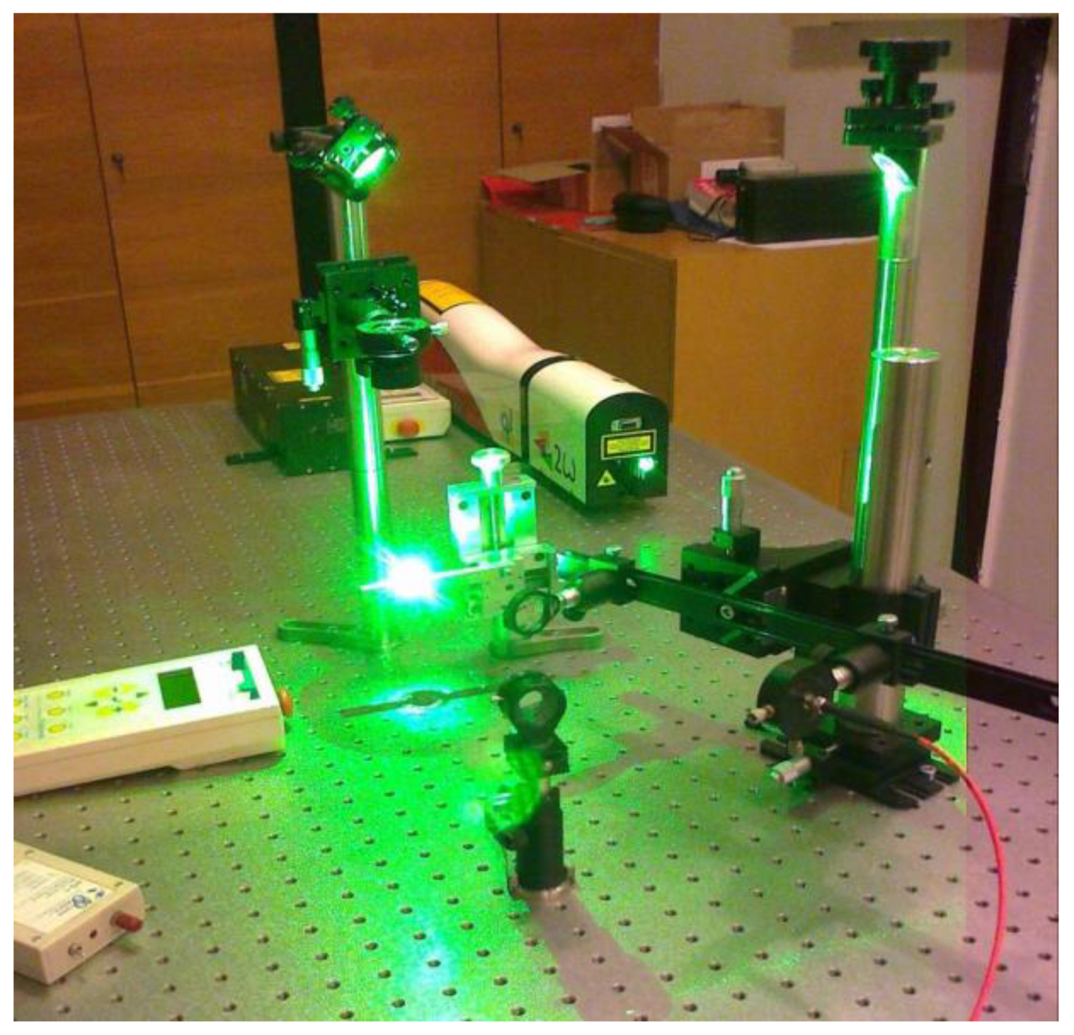
LIBS measurements were carried out using the apparatus from our recent studies [9,10]. Main parts of the used setup are a Q-switched pulsed Nd:YAG laser operated at the second harmonic frequency (532 nm, max. energy of 165 mJ per pulse, pulse duration of 4 ns, and repetition rate of 10 Hz), an emission spectrometer with an echelle grating (Mechelle ME 5000, Andor Technology) having the resolution λ/Δλ = 5000, an intensified CCD camera (iStar DH 734, Andor Technology), optical elements (Thorlabs), translation stage, and computer. Samples in the form of pressed pellets were placed on the translation stage. Spectra were taken as an accumulation of fifty laser shots from five different places on the sample surface, so five spectra were taken for each sample. Used delay time and exposition time were of 1 μs. All measurements were carried out in air atmosphere at the atmospheric pressure (as indicates in Figure 1). Before the data processing, all measured spectra were corrected according to the spectral response of our echelle spectrometer [23] and background noise measured at the same conditions as the LIBS spectra was also subtracted.

2.2. Zeolite Samples Preparation

Sodium form of zeolite Y was obtained from Research Institute of Petroleum and Hydrocarbon Gases, Bratislava. Ammonium form zeolite Y with chemical composition (70.4 wt. % of SiO₂, 25.0 wt. % of Al₂O₃, 4.2 wt. % of Na₂O, 0,4 wt. % of CaO, and trace amount of MgO) was prepared by the repeated ion exchange with 2M ammonium nitrate. The weight loss of the zeolite Y was 28.03%. The specific parameters of the used zeolite are summed up in

Table 1. Specific parameters of the used zeolite.

Surface Area (m2/g)	Volume of Micropores (cm3/g)	Pore Diameter (nm)	Acidity (mmol/g)
748	0.32	1.9–2.2	1.75

. CuSO₄.5H₂O (purity of 99.0%), Co(CH₃COO)₂.4H₂O (98.0%), K₂Cr₂O₇ (99.8%), PbNO₃ (99.0%), and CdCl₂ (99.0%) were used as a source of relevant metals (copper, cobalt, chromium, lead, and cadmium). Metals were loaded in amounts of 0.050 wt. %, 0.075 wt. %, 0.100 wt. %, 0.150 wt. %, and 0.500 wt. %. Solutions of a metal compound were prepared using the distilled water and desired amount of a chemical compound. Volume of the impregnation was made by wet way. Solution of a metal compound was blended with the powder zeolite and this suspension was mixed. Subsequently, the suspension was dried in an oven at a temperature of 90 °C for 3 h. Dried zeolite with a metal component was blended with inert paraffin on the amount of 30% in a vibration mill for 10 min. This material was transferred to the die to form a pellet. The die was placed in a press at a pressure of 10 MPa for 10 min. Obtained pellets were of dimensions of 20 mm in diameter and of 2 mm in thickness.

3. Results

3.1. Qualitative Analysis

The best signal to noise ratio was observed at the delay time (GD) and the exposure time (GW) of 1 μs. Except of these experimental conditions, other settings were also tested varying from 250–2500 ns, while the delay and exposure times were always equal (GD = GW). Several experimental conditions were tested to obtain the best experimental conditions, signal to noise ratio, possibility to observe both neutral and ionic lines of the elements of the interest in the LIBS spectra. Spectra were recorded in the wide spectral range of 200–975 nm. Due to the fact that plasma emission was collected using optical fiber linked to the entrance slit of spectrometer, spectral range between 200 nm and 220 nm was not used for analysis because the transmittance of the used fiber decreases rapidly in this range.

Apart from emission spectral lines of silicon, aluminum, and oxygen, which are the main components of zeolites, emission spectral lines of sodium, calcium, manganese, titanium, iron, nitrogen, and hydrogen were also observed in the LIBS spectra. Hydrogen and oxygen came both from the samples and from the ambient air atmosphere. Spectral lines of nitrogen originating from ambient air were observed, too. Presence of iron and titanium could come from the impurities of chemicals used in the process of zeolite synthesis.

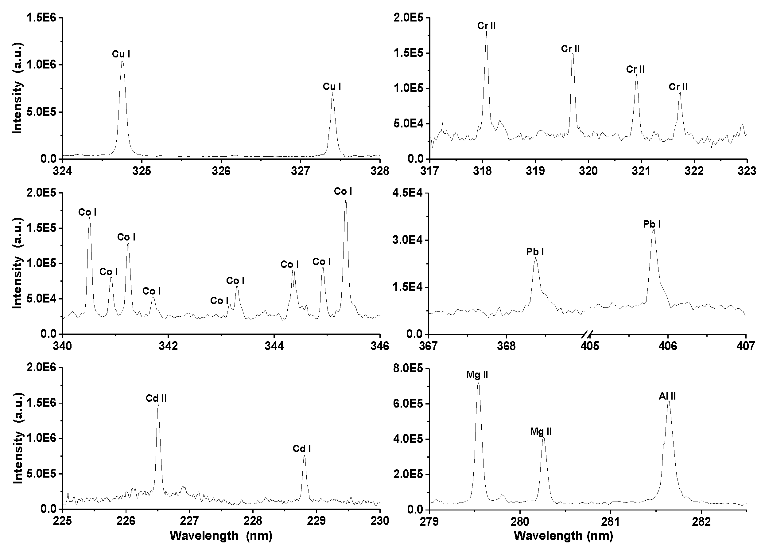
But the object of this research is the analysis of five heavy metals (Co, Cu, Cr, Cd, and Pb) contained in the prepared zeolite pellets. In the LIBS spectra of prepared pellets neutral spectral lines of lead and copper, neutral, and ionic spectral lines of cadmium, cobalt, and chromium were detected. Typical spectral lines of individual elements (some of them were used for construction of the calibration curves) are depicted in Figure 2. A blank sample was measured at the same experimental conditions for the purpose of verification of the presence of heavy metals. None of the elements of interest were detected in the blank sample.

3.2. Diagnostics of Laser-Induced Plasma

Two main plasma parameters were monitored during the data processing, i.e., the electron density N_e and the electron temperature T_e. The electron density was calculated from the Stark broadening of hydrogen H_α line (656.28 nm), resulting from the presence of chemically bounded water in the zeolite samples. There is also a contribution of air humidity as the experiments were carried out in air at atmospheric pressure. The equation with the full width at half area (FWHA) parameter was used because of its less sensitivity to ion dynamics [24].

$$\mathrm{FWHA}=0.549\mathrm{nm}\times {\left(\frac{N_e}{{10}^{23}{\mathrm{m}}^{-3}}\right)}^{0.67965},$$

(2)

where N_e is electron density.

The electron temperature was determined using multi-element Saha–Boltzmann plot method, well described in the research of Aguilera and Aragón [25], assuming that the plasma is in the local thermodynamic equilibrium (LTE). The well-known and frequently used McWhirter criterion

$$N_e\left(c{m}^{-3}\right)>1.6\times {10}^{12}\sqrt{T_e}{\left(\Delta E_{nm}\right)}^3$$

(3)

was applied for the determination if the plasma is in the state of LTE. In Equation (3), the symbol ΔE_nm indicates the highest energy level difference for which this criterion is still valid. This criterion represents only a necessary but not sufficient condition of LTE and is valid in the case of stationary and homogeneous plasma [26]. Despite this fact, a lot of authors used to apply this criterion for the verification if the analyzed plasma is in the state of LTE [27,28,29].

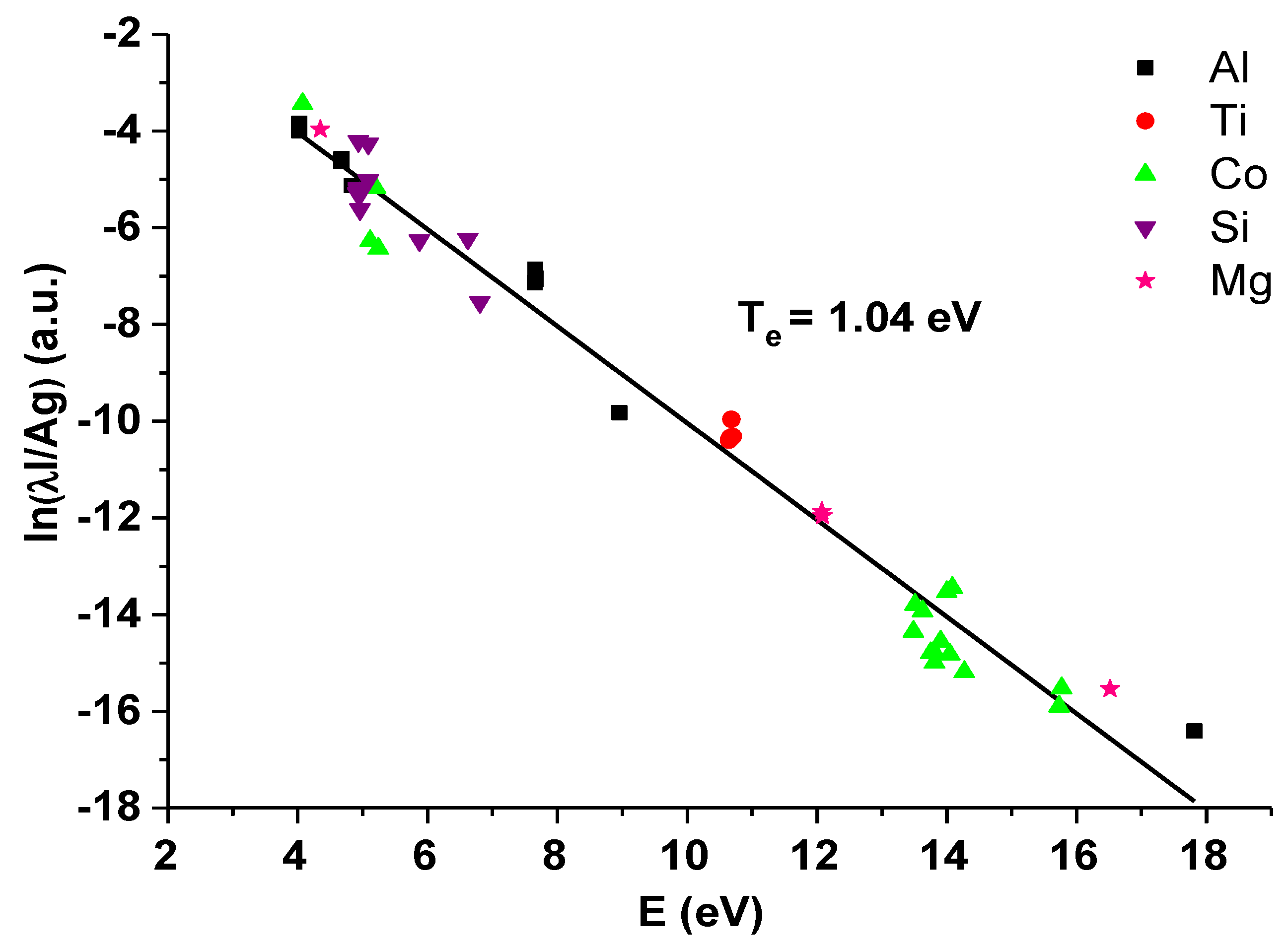
The example of multi-element Saha–Boltzmann plot is presented in Figure 3. For the electron temperature determination, the spectral lines of silicon, aluminum, cobalt, titanium, and magnesium were used, and the electron temperature of 1.04 eV (±0.02 eV) was calculated from the slope of the linear fit.

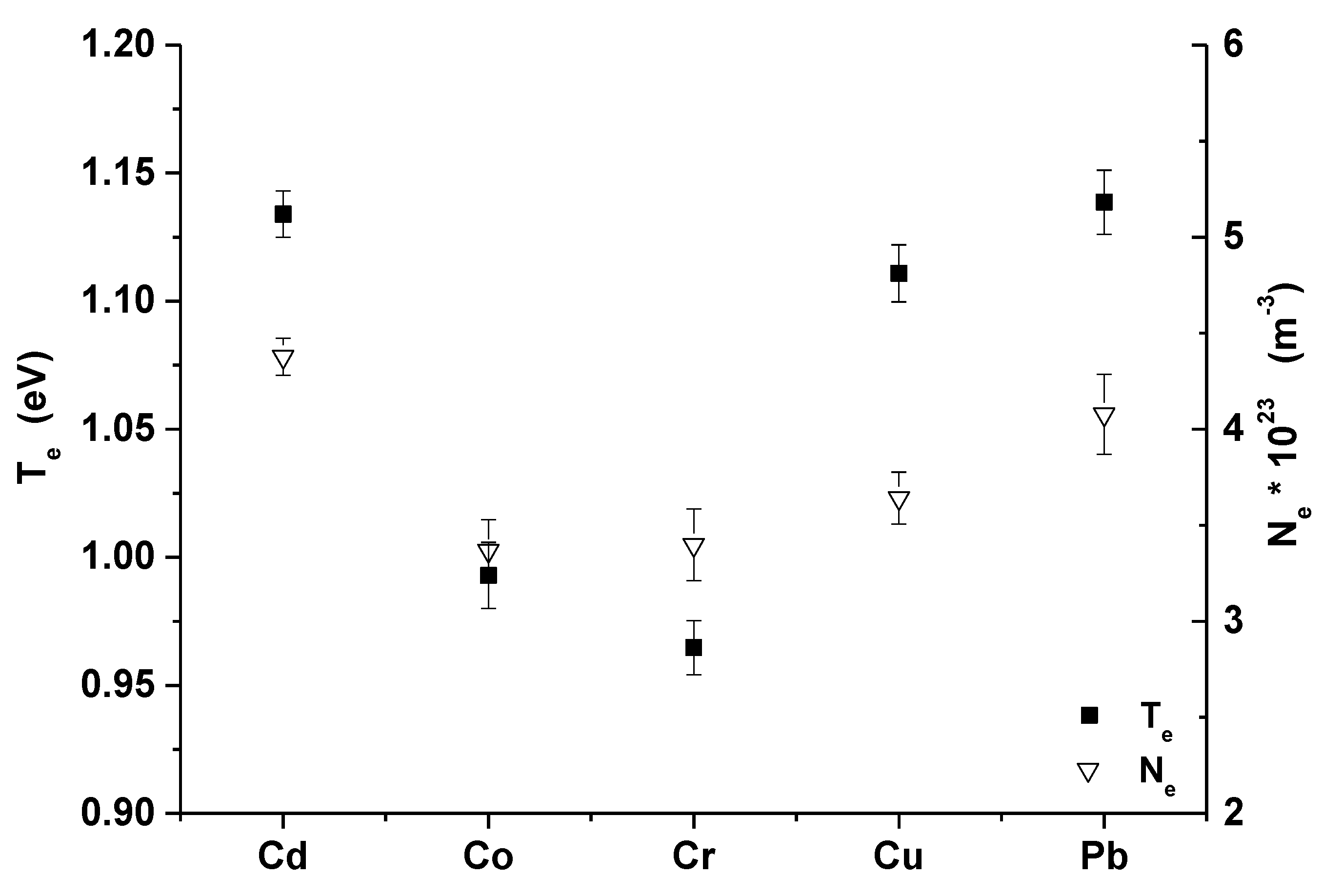
Figure 4 is showing the mean value and fluctuations of the electron density and temperature over all densities of heavy metals in the examined zeolite samples for Cd, Co, Cr, Cu, and Pb. Obtained electron densities were in the range of 3.25 × 10²³–4.55 × 10²³ m⁻³ and the electron temperatures were in the range of 0.95–1.18 eV.

3.3. Influence of the Ne and Te Fluctuation on the Plasma Composition

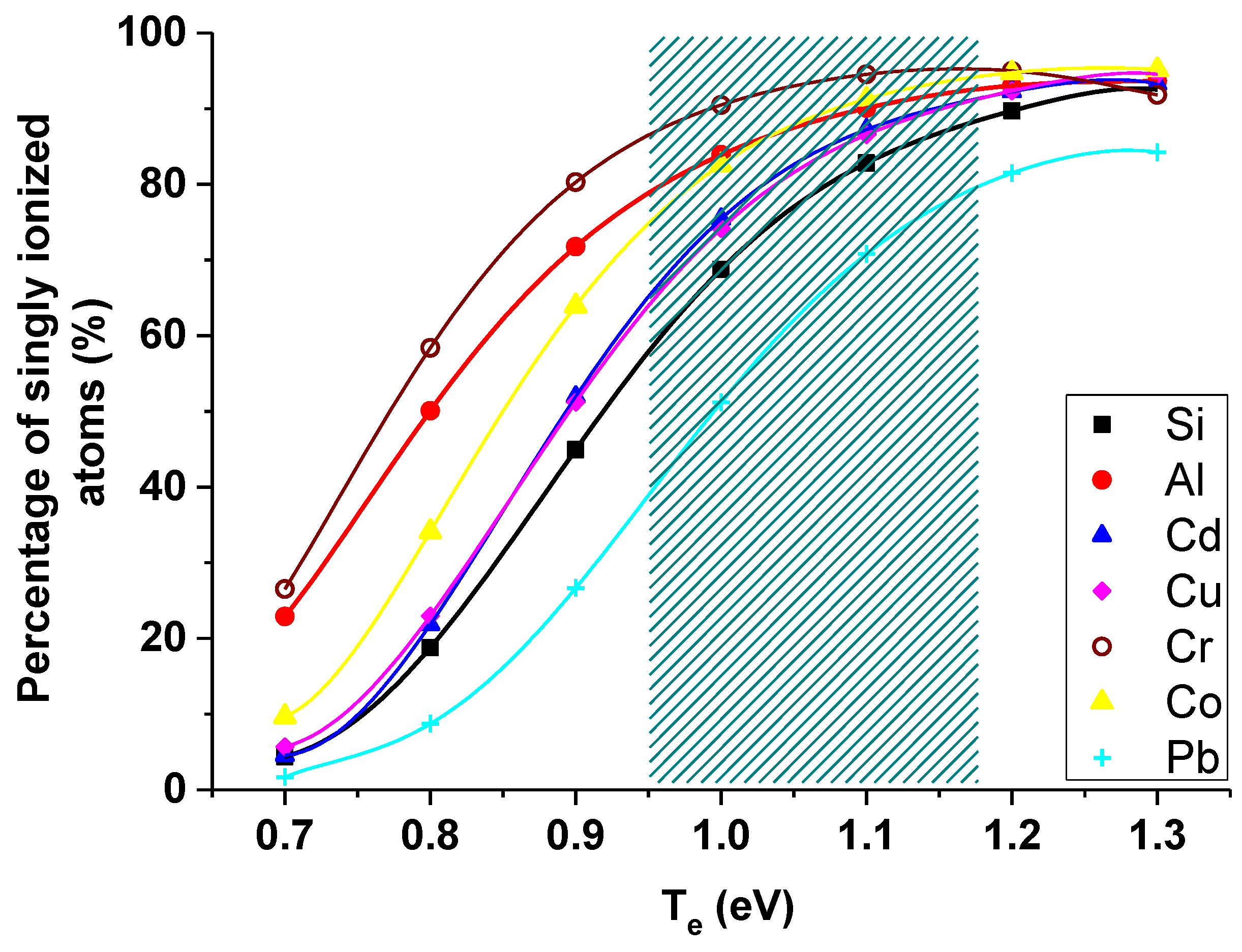
Influence of the electron temperature and electron density on the plasma composition was also monitored during the data processing by calculation of the ratio of singly ionized $N_S^{II}$ to neutral atom $N_S^I$ number densities of element s using charge-state distribution equation:

$$\frac{N_s^{II}}{N_s^I}=\frac{2Q_s^{II}\left(T_e\right)}{N_e{Q}_s^I\left(T_e\right)}\left(\frac{m_e{k}_B{T}_e}{2\pi {\hslash }^2}\right)exp\left(-\frac{E_s^{ion}}{k_B{T}_e}\right),$$

(4)

where Q_s is the partition function at the given electron temperature T_e, m_e is the electron mass, k_B is Boltzmann constant, $E_S^{ion}$ is the ionization energy of the elements.

The main part of plasma generated in our laboratory at the mentioned experimental conditions is formed by singly ionized atoms, usually 70–80% (for some elements, like Na or K, even more), the rest is formed by the neutral atoms. The number of doubly ionized atoms is negligible compared to the singly ionized and neutral atoms.

Figure 5 presents the percentage of singly ionized atoms in the temperature range of 0.7–1.3 eV and for the electron density of 3.8 × 10²³ m⁻³. Patterned part in the graph represents the electron temperature range obtained during our experiments. As it is clearly seen from Figure 5, the biggest variations of singly ionized atoms percentage over the obtained temperature range is for lead (from 40% to 80%).

3.4. Calibration Curves

Calibration curves represent the dependency between the integral intensity of a selected spectral line and the concentration of a given element. In some cases, a spectral line designated as an internal standard is used and then intensity ratio (intensity of selected spectral line/intensity of internal standard line) is plotted against an elemental concentration [30].

In our study, calibration curves were obtained using twenty-five zeolite samples containing heavy metals in known concentrations of copper, cobalt, chromium, cadmium, and lead. Each point in the calibration curve represents the average of five spectra taken from five different places on the sample surface.

The most commonly used method to compensate the dependence between the calibration curves and the plasma parameters, is to normalize the spectral line intensity (or integral intensity) of the element of interest to the intensity of the matrix spectral line or the buffer gas line intensity [30,31]. In our study, the heavy metals spectral lines (Cd, Co, Cr, Cu, Pb) were normalized to the spectral lines of the matrix (Si, Al, Mg, Ca). Moreover, reducing of the electron density fluctuations was achieved by the selection of the spectral lines of heavy metals and internal standard lines in the same degree of ionization. The influence of the electron temperature on the calibration curves was reduced by selecting of the spectral lines and the internal standard lines with a similar value of the upper energy levels and both elements should have also similar ionization energies (

Table 2. Specific parameters of used zeolite.

Element	Ionization Energy (eV)
Si	8.1517
Al	5.9858
Cu	7.7264
Cd	8.9938
Pb	7.4167
Co	7.881
Cr	6.7765
Mg	7.6462
Ca	6.1132

). Using the spectrometer with a narrow spectral range, the selected analyte and matrix lines should be close in the measured LIBS spectrum [31], which is not our case, because we were using a broadband echelle type spectrometer.

A group of neutral and ionic spectral lines of aluminum and silicon were selected as the internal standards. In the case of chromium, spectral lines of aluminum were selected as an internal standard, and in the case of cobalt, copper, cadmium, and lead, a group of silicon spectral lines were selected. Spectral lines were selected according to the mentioned parameters and are listed in

Table 3. Parameters of spectral lines used in the calibration curves (λ—wavelength of spectral line, A_ki—Einstein coefficient, E_i—energy of lower level, E_k—energy of upper level) [32,33].

Element	λ (nm)	Aki (s−1)	Ei (eV)	Ek (eV)
Si I	243.52	4.43 × 107	0.781	5.871
Si I	252.85	9.04 × 107	0.028	4.929
Si I	390.55	1.33 × 107	1.908	5.082
Cu I	515.32	6.00 × 107	3.786	6.192
Cu I	521.82	7.50 × 107	3.817	6.192
Cu I	324.75	1.39 × 108	0	3.817
Cd I	508.58	5.06 × 107	3.946	6.384
Pb I	283.31	5.92 × 107	0	4.375
Pb I	368.34	1.70 × 108	0.969	4.335
Pb I	405.78	9.10 × 107	1.321	4.375
Cr I	301.52	1.63 × 108	0.961	5.072
Cr I	301.37	8.30 × 107	0.968	5.081
Cr II	297.19	2.00 × 108	3.768	7.939
Cr II	312.50	8.19 × 107	2.455	6.421
Cr II	320.92	6.81 × 107	2.544	6.407
Co I	350.23	8.00 × 107	0.432	3.971
Co I	350.63	8.20 × 107	0.514	4.049
Co I	351.26	1.00 × 108	0.582	4.11
Co II	258.72	1.19 × 108	1.328	6.118
Co II	258.22	1.40 × 108	1.404	6.204
Co II	236.38	2.10 × 108	0.499	5.743
Co II	239.74	2.40 × 108	1.217	6.387
Al I	305.71	7.50 × 107	3.613	7.668
Al II	281.62	3.83 × 108	7.421	11.822
Mg II	280.27	2.57 × 108	0	4.422
Ca II	393.37	1.47 × 108	0	3.151

.

To achieve a higher precision (regression coefficient and slope of the linear fit) of calibration curves, in some cases more than one spectral line were selected for the calibration curve construction.

3.4.1. Copper

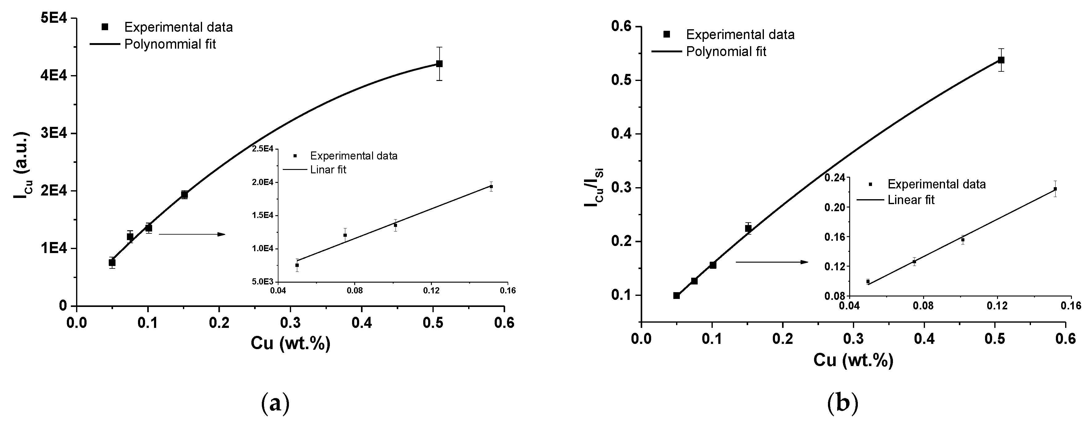
For the calibration curves construction, usually resonant Cu I lines at 324.75 nm are used [34,35]. In Figure 6, calibration curves obtained by fitting of Cu I 324.75 nm are depicted. Both cases were studied, i.e., with the use of an internal standard-zeolite matrix silicon Si I line at 243.52 nm and without the use of this line. Silicon line Si I 243.52 nm was used according to its parameters, i.e., the energy of upper level and the ionization energy of both elements; similar to the Cu I 324.75 nm line (see Table 2 and Table 3). However, as it is clearly seen from Figure 6a,b, the use of this line often leads to a nonlinear behavior of the calibration curves already at very low concentrations of Cu in the analyzed sample. This can be an indication of the presence of self-absorption of the Cu line.

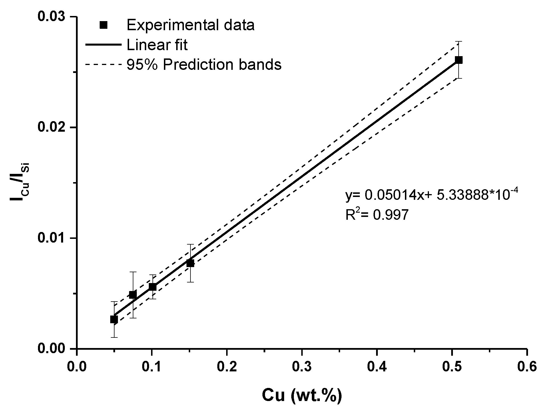
Therefore, non-resonant Cu I spectral lines at 515.32 nm and 521.82 nm were selected for the calibration curves construction. A calibration curve obtained using these two lines, is depicted in Figure 7. As an internal standard, Si I 243.52 nm line was used. Ionic spectral lines Cu II were not observed in the measured LIBS spectra.

3.4.2. Cadmium

In the LIBS spectra, both neutral Cd I (228.80 nm, 346.62 nm, 361.05 nm, and 508.58 nm) and ionic Cd II (226.50 nm) spectral lines were observed. For the calibration curve construction, a non-resonant spectral line at 508.58 nm was selected. As an internal standard, silicon Si I spectral line at 243.52 nm was selected, similarly as in the case of copper.

3.4.3. Lead

In the case of lead, several neutral spectral lines (Pb I; 261.42 nm, 283.31 nm, 368.34 nm, and 405.78 nm) were observed in the measured LIBS spectra, ionic spectral lines were not detected. For the calibration curve construction, three Pb I spectral lines (283.31 nm, 368.34 nm, and 405.78 nm) were used. As an internal standard, Si I spectral line at 390.55 nm was used. Spectral lines were selected according to the very similar energies of upper level and ionization energies of both elements. Use of several spectral lines instead of only one line has led to the significant improvement in the regression coefficient and intercept of the calibration curve with the y axis.

3.4.4. Cobalt

In the case of cobalt, calibration curves were obtained both from neutral and ionic spectral lines. Three neutral spectral lines of cobalt (Co I; 350.23 nm, 350.63 nm, and 351.26 nm) were used for the calibration curve construction. As an internal standard, neutral line of silicon Si I at 252.85 nm was selected. Used spectral lines have close values of energies of upper levels.

Calibration curve obtained using ionic spectral lines of cobalt was constructed using four spectral lines (Co II; 236.38 nm, 239.74 nm, 258.22 nm, and 258.72 nm). As an internal standard, ionic spectral lines of calcium (Ca II; 393.37 nm) and magnesium (Mg II; 280.27 nm) were used.

3.4.5. Chromium

The LIBS spectra of zeolite pellets containing chromium are characterized by a high number of both chromium neutral and ionic spectral lines, as in the case of cobalt. Chromium has similar ionization energy to aluminum. Therefore, spectral lines of this element were selected as internal standards. Calibration curves were constructed both for neutral atoms and ions. For the calibration curves, two neutral chromium (Cr I; 301.37 nm and 301.52 nm) lines were used. As the internal standard line, aluminum spectral line (Al I; 305.71 nm) was used. In the case of ionic chromium, three spectral lines (Cr II; 297.19 nm, 312.5 nm, and 320.92 nm) were used and as the internal standard, aluminum line (Al II; 281.62 nm) was used. Fitting parameters of the obtained calibration curves of all elements are summed up in

Table 4. Fitting parameters of the linear calibration curves.

Calibration Curve	Line Type	Line Wavelength (nm)	Sensitivity (wt.% −1)	R2	LOD (ppm)
Cu I/Si I	neutral	324.75	1.262	0.995
Cu I/Si I	2 neutral lines	515.32; 521.82	0.05	0.997
Cu I	neutral	324.75	111327	0.956	14.4
Cd I/Si I	neutral	508.58	1.745	0.995
Cd II	ionic	226.5	20.821	0.986	190.7
Pb I/Si I	3 neutral lines	283.31; 368.34; 405.78	0.174	0.999
Pb I	neutral	405.78	150.86	0.937	62.6
Co I/Si I	3 neutral lines	350.23; 350.63; 351.26	1.66	0.993
Co II/Mg II + Ca II	4 ionic lines	236.38; 239.74; 258.22; 258.72	1.638	0.998
Co I	neutral	348.94	154.49	0.974	18.5
Cr I/Al I	2 neutral lines	301.37; 301.52	1.634	0.997
Cr II/Al II	3 ionic lines	297.19; 312.5; 320.92	1.776	0.999
Cr I	neutral	425.43	2462253	0.994	16.4

.

3.5. Limits of Detection

Limit of detection (LOD) represents the lowest elemental concentration which can be detected by the given apparatus and at the given experimental conditions. For the detection limit calculation following formula,

$$LOD=\frac{3\sigma }{S}$$

(5)

was used, where σ designates the standard deviation of the background and S is slope of the calibration curve linear fit. Obtained detection limits for all analysed heavy metals compared to the LOD found in the literature are summed up in

Table 5. Limits of detection of five heavy metals.

Element	Line (nm)	Matrix	LOD	Ref.
Cd I	228.80	soil	6 μg/g	[36]
Cd II	214.44	ice	1.4 mg/L	[16]
Cd II	214.44	water	7.1 mg/L	[16]
Cd II	226.50	zeolite	190.7 ppm	this research
Cr I	425.22	steel	24 ppm	[37]
Cr I	425.43	soil	2.5 μg/g	[38]
Cr I	425.43	water	10 μg/mL	[39]
Cr I	425.43	soil	2 mg/kg	[40]
Cr I	425.43	oil	20 μg/mL	[39]
Cr I	425.43	soil	8 ppm	[37]
Cr II	267.72	steel	6 ppm	[37]
Cr II	283.56	water	30 ppm	[36]
Cr II	283.56	oil	0.4 μg/mL	[39]
Cr II	283.56	water	100 ppb	[37]
Cr II	284.33	water	42 ppm	[36]
Cr II	267.72	ice	1.4 mg/L	[16]
Cr II	267.72	water	10.5 mg/L	[16]
Cr I	360.53	oil	10.59 μg/g	[41]
Cr I	425.43	zeolite	16.4 ppm	this research
Cu I	324.75	Al alloy	10 ppm	[37]
Cu I	324.75	Al alloy	17.49 ppm	[42]
Cu I	324.75	ice	2.3 mg/L	[16]
Cu I	324.75	oil	5 μg/mL	[39]
Cu I	324.75	steel alloy	6.31 ppm	[43]
Cu I	324.75	water	7 ppm	[37]
Cu I	324.75	water	7 μg/mL	[39]
Cu I	324.75	water	9.6 mg/L	[16]
Cu I	324.75	soil	3.3 μg/g	[38]
Cu I	324.75	oil	2.87 μg/g	[41]
Cu I	324.75	zeolite	14.4 ppm	this research
Pb I	363.96	bronze	0.30%	[31]
Pb I	405.78	concrete	10 ppm	[37]
Pb I	405.78	soil	5 ppm	[37]
Pb I	405.78	soil	17 μg/g	[38]
Pb I	405.78	ice	1.3 mg/L	[16]
Pb I	405.78	water	100 μg/mL	[39]
Pb I	405.78	water	12.5 mg/L	[16]
Pb I	405.78	soil	20 ppm	[44]
Pb I	405.78	oil	90 μg/mL	[39]
Pb I	405.78	oil	>100 μg/g	[41]
Pb I	405.78	sediments	190 μg/g	[45]
Pb I	261.42	CaCO3	95 ppm	[46]
Pb I	405.78	zeolite	62.6 ppm	this research
Co I	350.23	W-carbide	4% m/m	[47]
Co I	345.35	Cu concentrate	884 ppm	[48]
Co I	348.94	zeolite	18.5 ppm	this research

.

4. Conclusion

Twenty-five zeolite samples containing heavy metals, i.e., copper, cadmium, cobalt, chromium, and lead, in the concentration range of 0.05–0.5 wt.% were analyzed using the laser induced breakdown spectroscopy in order to obtain the calibration curves and the detection limits of mentioned heavy metals.

Important plasma parameters, i.e., electron density and temperature, were monitored during all data processing. For the electron density calculation, Stark broadening of hydrogen line was used, and for the determination of the electron temperature, a method of multi-element Saha–Boltzmann plots was applied. Furthermore, a representation of neutral and singly ionized atoms in the LIBS plasma was monitored using charge-state distribution equation.

For the calibration curves, construction spectral lines of silicon (in the case of cobalt Co I, copper, cadmium, and lead), aluminum (in the case of chromium), and calcium Ca II together with the magnesium Mg II (in the case of Co II) were selected as the internal standards. Using the internal standards to suppress the fluctuation of intensity between spectra, the regression coefficients and the intercepts of a linear fit of the data points in the calibration graphs were significantly improved. Moreover, summary of the selected lines of the studied elements increases the precision with which we can calculate the concentration of the element in an unknown sample. Summing only the non- resonant spectral lines, resonant lines were removed from the list to decrease the influence of an even small self-absorption effect.

On the other hand, LOD, as it is defined, gives us information whether the element is present in the sample or not. Therefore summarizing spectral lines is not a possibility in this case. Hence, in the case of LOD determination, resonant spectral lines were selected in the most cases. The obtained LODs for each heavy metal are present in Table 5. Obtained values of LOD could be better, but we wanted to use spectra (the spectra with reliable number of accumulations) that were used for calculation of calibration curves for the evaluation of LOD. Increasing the amount of laser shots accumulated into one spectrum would increase the ratio amplitude of a resonant line to standard deviation of the noise and would eventually decrease LOD. Therefore, the LODs presented in this paper are the ones that can be obtained with standard LIBS spectra with a reasonable number of accumulations.

Obtained detection limits are comparable with those found in the literature, except of cadmium. In this case, a relatively high detection limit can be caused due to the use of an optical fiber for the guidance of plasma emission to the entrance slit of the spectrometer. The optical fiber decreases sensitivity and increases noise level. Therefore, in our experimental configuration, Cd I 228.80 nm and Cd II 226.50 nm lines are not suitable for the determination of the detection limits.

Furthermore, the use of an echelle type of spectrometer limits the possibility to obtain better detection limits due to the shape of the calibration curve. In the case a spectral line is located at the interface of two adjacent orders, where the sensitivity of the spectrometer can decrease to 20% or less of the original value, the intensity of such a line will be influenced by this fact. Therefore, spectral lines must be selected carefully in order to be not located at the interface of two adjacent orders.

References

- Meier, W.M. Zeolites and zeolite-like materials. Pure Appl. Chem. 1986, 58, 1323–1328. [Google Scholar] [CrossRef]
- Weitkamp, J. Zeolites and catalysis. Solid State Ionics 2000, 131, 175–188. [Google Scholar] [CrossRef]
- Jehlička, J.; Vandenabeele, P.; Edwards, H.G.M. Discrimination of zeolites and beryllium containing silicates using portable Raman spectroscometric equipment with near-infrared excitation. Spectrochim. Acta Part A 2012, 86, 341–346. [Google Scholar] [CrossRef] [PubMed]
- Querol, X.; Moreno, N.; Uman, J.C.; Juan, R.; Hernandez, S.; Fernandez-Pereira, C.; Ayora, C.; Janssen, M.; García-Martínez, J.; Linares-Solano, A.; et al. Application of zeolitic material synthesised from fly ash to the decontamination of waste water and flue gas. J. Chem. Technol. Biotechnol. 2002, 77, 292–298. [Google Scholar] [CrossRef]
- Motsi, T.; Rowson, N.A.; Simmons, M.J.H. Adsorption of heavy metals from acid mine drainage by natural zeolite. Int. J. Miner. Process. 2009, 92, 42–48. [Google Scholar] [CrossRef]
- Ferreira, L.; Fonseca, A.M.; Botelho, G.; Almeida-Aguiar, C.; Neves, I.C. Antimicrobial activity of faujasite zeolites doped with silver. Microporous Microporous Mat. 2012, 160, 126–132. [Google Scholar] [CrossRef]
- Pitcher, S.K.; Slade, R.C.T.; Ward, N.I. Heavy metal removal from motorway storm water using zeolites. Sci. Total. Environ. 2004, 334–335, 161–166. [Google Scholar] [CrossRef]
- Shi, W.; Shao, H.; Li, H.; Shao, M.; Du, S. Progress in the remediation of hazardous heavy metal-polluted soils by natural zeolite. J. Hazard. Mater. 2009, 170, 1–6. [Google Scholar] [CrossRef]
- Horňáčková, M.; Grolmusová, Z.; Horňáček, M.; Rakovský, J.; Hudec, P.; Veis, P. Calibration analysis of zeolites by laser induced breakdown spectroscopy. Spectrochim. Acta B 2012, 74, 119–123. [Google Scholar] [CrossRef]
- Horňáčková, M.; Horňáček, M.; Rakovský, J.; Hudec, P.; Veis, P. Determination of Si/Al molar ratios in microporous zeolites using calibration-free laser induced breakdown spectroscopy. Spectrochim. Acta B 2013, 88, 69–74. [Google Scholar] [CrossRef]
- Kaiser, J.; Galiová, M.; Novotný, K.; Červenka, R.; Reale, L.; Novotný, J.; Liška, M.; Samek, O.; Kanický, V.; Hrdlička, A.; et al. Mapping of lead, magnesium and copper accumulation in plant tissues by laser-induced breakdown spectroscopy and laser-ablation inductively coupled plasma mass spectrometry. Spectrochim. Acta B 2009, 64, 67–73. [Google Scholar] [CrossRef]
- Manzoor, S.; Moncayo, S.; Navarro-Villoslada, F.; Ayala, J.A.; Izquierdo-Hornillos, R.; Manuel de Villena, F.J.; Caceres, J.O. Rapid identification and discrimination of bacterial strains by laser induced breakdown spectroscopy and neural networks. Talanta 2014, 121, 65–70. [Google Scholar] [CrossRef] [PubMed]
- Dell’Aglio, M.; De Giacomo, A.; Gaudiuso, R.; De Pascale, O.; Senesi, G.S.; Longo, S. Laser Induced Breakdown Spectroscopy applications to meteorites: Chemical analysis and composition profiles. Geochim. Cosmochim. Acta 2010, 74, 7329–7339. [Google Scholar] [CrossRef]
- Kiros, A.; Lazic, V.; Gigante, G.E.; Gholap, A.V. Analysis of rock samples collected from rock hewn churches of Lalibela, Ethiopia using laser-induced breakdown spectroscopy. J. Archaeol. Sci. 2013, 40, 2570–2578. [Google Scholar] [CrossRef]
- Haider, A.F.M.Y.; Ullah, M.H.; Khan, Z.H.; Kabir, F.; Abedin, K.M. Detection of trace amount of arsenic in groundwater by laser-induced breakdown spectroscopy and adsorption. Opt. Laser Technol. 2014, 56, 299–303. [Google Scholar] [CrossRef]
- Sobral, H.; Sanginés, R.; Trujillo-Vázquez, A. Detection of trace elements in ice and water by laser-induced breakdown spectroscopy. Spectrochim. Acta B 2012, 78, 62–66. [Google Scholar] [CrossRef]
- Järvinen, S.T.; Saarela, J.; Toivonen, J. Detection of zinc and lead in water using evaporative preconcentration and single-particle laser-induced breakdown spectroscopy. Spectrochim. Acta B 2013, 86, 55–59. [Google Scholar] [CrossRef]
- Gondal, M.A.; Hussain, T. Determination of poisonous metals in wastewater collected from paint manufacturing plant using laser-induced breakdown spectroscopy. Talanta 2007, 71, 73–80. [Google Scholar] [CrossRef]
- Senesi, G.S.; Dell’Aglio, M.; Gaudiuso, R.; De Giacomo, A.; Zaccone, C.; De Pascale, O.; Miano, T.M.; Capitelli, M. Heavy metal concentrations in soils as determined by laser-induced breakdown spectroscopy (LIBS), with special emphasis on chromium. Environ. Res. 2009, 109, 413–420. [Google Scholar] [CrossRef]
- Camacho, J.J.; Vrabel, J.; Manzoor, S.; Pérez-Arribas, L.V.; Díaz, D.; Caceres, J.O. Spatiotemporal diagnostics of laser induced plasma of potassium gallosilicate zeolite. J. Anal. At. Spectrom 2019, 34, 1247–1255. [Google Scholar] [CrossRef]
- Bocková, J.; Tian, Y.; Yin, H.; Delepine-Gilon, N.; Chen, Y.; Veis, P.; Yu, J. Determination of Metal Elements in Wine Using Laser-Induced Breakdown Spectroscopy (LIBS). Appl. Spectrosc. 2017, 71, 1–10. [Google Scholar] [CrossRef] [PubMed]
- Bocková, J.; Marín-Roldán, A.; Yu, J.; Veis, P. Potential use of surface-assisted LIBS for determination of strontium in wines. Appl. Optics 2018, 57, 8272–8278. [Google Scholar] [CrossRef] [PubMed]
- Rakovský, J.; Krištof, J.; Čermák, P.; Kociánová, M.; Veis, P. Measurement of echelle spectrometer spectral response in UV. In Proceedings of Contributed Papers Part II: Physics of Plasma and Ionized Media, 20th Annual Student Conference WDS’ 11, Prague, Czech Republic, 31 May–3 June 2011; Šafránková, J., Pavlu, J., Eds.; Matfyzpress: Prague, Czech Republic, 2011; pp. 257–262. [Google Scholar]
- Gigosos, M.A.; González, M.A.; Cardenoso, V. Computer simulated Balmer-alpha, -beta and -gamma Stark line profiles for non-equilibrium plasmas diagnostics. Spectrochim. Acta B 2003, 58, 1489–1504. [Google Scholar] [CrossRef]
- Aguilera, J.A.; Aragón, C. Multi-element Saha–Boltzmann and Boltzmann plots in laser-induced plasmas. Spectrochim. Acta B 2007, 62, 378–385. [Google Scholar] [CrossRef]
- Cristoforetti, G.; De Giacomo, A.; Dell’Aglio, M.; Legnaioli, S.; Tognoni, E.; Palleschi, V.; Omenetto, N. Local Thermodynamic Equilibrium in Laser-Induced Breakdown Spectroscopy: Beyond the McWhirter criterion. Spectrochim. Acta B 2010, 65, 86–95. [Google Scholar] [CrossRef]
- Praher, B.; Palleschi, V.; Viskup, R.; Heitz, J.; Pedarnig, J.D. Calibration free laser-induced breakdown spectroscopy of oxide materials. Spectrochim. Acta B 2010, 65, 671–679. [Google Scholar] [CrossRef]
- Rauschenbach, I.; Lazic, V.; Pavlov, S.G.; Hübers, H.W.; Jessberger, E.K. Laser induced breakdown spectroscopy on soils and rocks: Influence of the sample temperature, moisture and roughness. Spectrochim. Acta B 2008, 63, 1205–1215. [Google Scholar] [CrossRef]
- Ma, Q.L.; Motto-Ros, V.; Lei, W.Q.; Boueri, M.; Zheng, L.J.; Zeng, H.P.; Bar-Matthews, M.; Ayalon, A.; Panczer, G.; Yu, J. Multi-elemental mapping of a speleothem using laser-induced breakdown spectroscopy. Spectrochim. Acta B 2010, 65, 707–714. [Google Scholar] [CrossRef]
- Lasheras, R.J.; Bello-Gálvez, C.; Anzano, J.M. Quantitative analysis of oxide materials by laser-induced breakdown spectroscopy with argon as an internal standard. Spectrochim. Acta B 2013, 82, 65–70. [Google Scholar] [CrossRef]
- Elhassan, A.; Cristoforetti, G.; Legnaioli, S.; Palleschi, V.; Salvetti, A.; Tognoni, E.; Ingo, G.; Harith, M.A. LIBS Calibration Curves and Determination of Limits of Detection (LOD) in Single and Double Pulse Configuration for Quantitative LIBS Analysis of Bronzes. In Strategies for Saving Our Cultural Heritage, Cairo, Egypt, 25 February–1 March 2007; Argyropoulos, V., Hein, A., Harith, M.A., Eds.; TEI of Athens: Athens, Greece, 2007; pp. 72–77. [Google Scholar]
- Kramida, A.; Ralchenko, Y.; Reader, J.; NIST ASD Team. NIST Atomic Spectra Database (version 5.1). National Institute of Standards and Technology, Gaithersburg, MD; 2013. Available online: http://physics.nist.gov/asd (accessed on 21 March 2019).
- Kurucz, R.L.; Bell, B. Kurucz CD-ROM No. 23. Atomic Line Data; Smithsonian Astrophysical Observatory: Cambridge, MA, USA, 1995. [Google Scholar]
- Garcimunon, M.; Díaz Pace, D.M.; Bertuccelli, G. Laser-induced breakdown spectroscopy for quantitative analysis of copper in algae. Opt. Laser Technol. 2013, 47, 26–30. [Google Scholar] [CrossRef]
- Liu, Y.; Bousquet, B.; Baudelet, M.; Richardson, M. Improvement of the sensitivity for the measurement of copper concentrations in soil by microwave-assisted laser-induced breakdown spectroscopy. Spectrochim. Acta B 2012, 73, 89–92. [Google Scholar] [CrossRef] [Green Version]
- Rai, N.K.; Rai, A.K. LIBS—An efficient approach for the determination of Cr in industrial wastewater. J. Hazard. Mater. 2008, 150, 835–838. [Google Scholar] [CrossRef] [PubMed]
- Miziolek, A.W.; Palleschi, V.; Schechter, I. Laser Induced Breakdown Spectroscopy: Fundamental and Application; Cambridge University Press: New York, NY, USA, 2006; ISBN 978-0-511-24529-9. [Google Scholar]
- Hilbk-Kortenbruck, F.; Noll, R.; Wintjens, P.; Falk, H.; Becker, C. Analysis of heavy metals in soils using laser-induced breakdown spectrometry combined with laser-induced fluorescence. Spectrochim. Acta B 2001, 56, 933–945. [Google Scholar] [CrossRef]
- Fichet, P.; Mauchien, P.; Wagner, J.F.; Moulin, C. Quantitative elemental determination in water and oil by laser induced breakdown spectroscopy. Anal. Chim Acta 2001, 429, 269–278. [Google Scholar] [CrossRef]
- Gondal, M.A.; Hussain, T.; Yamani, Z.H.; Baig, M.A. On-line monitoring of remediation process of chromium polluted soil using LIBS. J. Hazard. Mater. 2009, 163, 1265–1271. [Google Scholar] [CrossRef] [PubMed]
- Xiu, J.; Motto-Ros, V.; Panczer, G.; Zheng, R.; Yu, J. Feasibility of wear metal analysis in oils with parts per million and sub-parts per million sensitivities using laser-induced breakdown spectroscopy of thin oil layer on metallic target. Spectrochim. Acta B 2014, 91, 24–30. [Google Scholar] [CrossRef]
- Mohamed, W.T.Y. Improved LIBS limit of detection of Be, Mg, Si, Mn, Fe and Cu in aluminum alloy samples using a portable Echelle spectrometer with ICCD camera. Opt Laser Technol. 2008, 40, 30–38. [Google Scholar] [CrossRef]
- Ismail, M.A.; Imam, H.; Elhassan, A.; Youniss, W.T.; Harith, M.A. LIBS limit of detection and plasma parameters of some elements in two different metallic matrices. J. Anal. At. Spectrom. 2004, 19, 489–494. [Google Scholar] [CrossRef]
- Burakov, V.S.; Tarasenko, N.V.; Nedelko, M.I.; Kononov, V.A.; Vasilev, N.N.; Isakov, S.N. Analysis of lead and sulfur in environmental samples by double pulse laser induced breakdown spectroscopy. Spectrochim. Acta B 2009, 64, 141–146. [Google Scholar] [CrossRef]
- Cunat, J.; Fortes, F.J.; Laserna, J.J. Real time and in situ determination of lead in road sediments using a man-portable laser-induced breakdown spectroscopy analyser. Anal. Chim. Acta 2009, 633, 38–42. [Google Scholar] [CrossRef]
- Samek, O.; Beddows, D.C.S.; Telle, H.H.; Kaiser, J.; Liska, M.; Caceres, J.O.; Gonzales Urena, A. Quantitative laser-induced breakdown spectroscopy analysis of calcified tissue samples. Spectrochim. Acta B 2001, 56, 865–875. [Google Scholar] [CrossRef]
- Novotný, K.; Staňková, A.; Häkkänen, H.; Korppi-Tommola, J.; Otruba, V.; Kanický, V. Analysis of powdered tungsten carbide hard-metal precursors and cemented compact tungsten carbides using laser-induced breakdown spectroscopy. Spectrochim. Acta B 2007, 62, 1567–1574. [Google Scholar] [CrossRef]
- Lazarek, L.; Antonczak, A.J.; Wójcik, M.R.; Drzymala, J.; Abramski, K.M. Evaluation of the laser-induced breakdown spectroscopy technique for determination of the chemical composition of copper concentrates. Spectrochim. Acta B 2014, 97, 74–78. [Google Scholar] [CrossRef]
Figure 1.
Laser spark created above the sample surface.
Figure 2.
Spectral lines of elements (copper, chromium, cobalt, magnesium, aluminum, cadmium, and lead) identified in the laser-induced breakdown spectroscopy (LIBS) spectra of zeolite.
Figure 3.
Multi-element Saha–Boltzmann plot for the zeolite containing 0.5 wt.% of Co (where on the vertical axis I is the line intensity, λ is the wavelength of the used spectral line, A is the Einstein coefficient, and g is degeneracy of the energy level).
Figure 4.
Mean value and fluctuations of the plasma parameters over all samples (error bars represent average standard deviation of evaluated Te and Ne).
Figure 5.
Number of singly ionized atoms in the temperature range of 0.7–1.3 eV and for the average electron density of 3.8 × 10²³ m−3 (patterned part corresponds with the obtained range of Te).
Figure 6.
(a) Calibration curves of copper obtained using of Cu I 324.75 nm line and linear fit of first four data points; (b) calibration curve of Cu I 324.75 nm line with using of Si I line as an internal standard and linear fit of first four data points (error bars represent relative standard deviation (RSD) of used data).
Figure 7.
Calibration curve of copper obtained using Cu I: 515.32 and 521.82 nm lines (error bars represent relative standard deviation (RSD) of used data).