MEMS-Based Cantilever Sensor for Simultaneous Measurement of Mass and Magnetic Moment of Magnetic Particles

Abstract

This study presents a measurement approach suitable for the simultaneous determination of both the mass m_p and magnetic moment µ_p of magnetic particles deposited on a micro electro mechanical system (MEMS) resonant cantilever balance, which is operated in parallel to an external magnetic field-induced force gradient F′(z). Magnetic induction B(z) and its second spatial derivative δ²B/δz² is realized, beforehand, through the finite element method magnetics (FEMM) simulation with a pair of neodymium permanent magnets configured in a face-to-face arrangement. Typically, the magnets are mounted in a magnet holder assembly designed and fabricated in-house. The resulting F′ lowers the calibrated intrinsic stiffness k₀ of the cantilever to k₀-F′, which can, thus, be obtained from a measured resonance frequency shift of the cantilever. The magnetic moment µ_p per deposited particle is determined by dividing F′ by δ²B/δz² and the number of the attached monodisperse particles given by the mass-induced frequency shift of the cantilever. For the plain iron oxide particles (250 nm) and the magnetic polystyrene particles (2 µm), we yield µ_p of 0.8 to 1.5 fA m² and 11 to 19 fA m² compared to 2 fA m² and 33 fA m² nominal values, respectively.

1. Introduction

The merit of magnetic particles (MPs) and their diverse and widespread applications is an ever-present reality that continues to trigger endless possibilities. These particle types have, for instance, greatly revolutionized many fields of science and technology, including biomedicine and environmental monitoring. MPs often serve as magnetic separation tools in effluent processing for contaminants removal, remediation and water treatment [1,2]. They also primarily serve as diagnostic tools [3,4], e.g., as contrast enhancement gents and as tracers for magnetic resonance imaging (MRI) and magnetic particle imaging (MPI) processes, respectively. Their appreciable use is quite evident in the targeted delivery of therapeutic drugs, gene and radionuclides, magnetic hyperthermia (for the treatment of tumors), treatment of iron deficiency, magnetic separation of biomolecules such as proteins, cells, antibodies and bacteria and as magnetic markers (for biosensing) [1,2,5,6,7,8,9,10]. For a successful and versatile application, knowledge of the magnetic properties of these particles (e.g., particle size, the chemical nature of magnetic material, magnetic content, saturation magnetization) is essential and influential. Magnetic particles are easily manipulated by applying a sufficiently high external magnetic field, which tends to align the particle’s magnetic moment(s) with the magnetizing field. In addition, if the latter is turned off, the magnetic dipole moments begin to randomize, thereby reducing the bulk magnetization [7].

The detection and characterization of magnetic particles deploy several techniques. Notwithstanding, various methods are utilized for the colloidal and physicochemical characterization of MPs. This consists of electrical conductivity measurements, a thermogravimetric analysis (TGA), scanning electron microscopy (SEM), transmission electron microscopy (TEM), X-ray diffraction (XRD) technique, Fourier transform infrared spectroscopy (FTIR) and atomic absorption spectroscopy (AAS). Thermogravimetric analysis has, for instance, been described as an effective chemical composition measurement method for quantitative determination of the mass content and magnetic content percentages of MPs [11,12,13]. Other magnetic particle characterization approaches include optical methods (e.g., dynamic light scattering), the AC susceptibility method, nuclear magnetic resonance (NMR) spectroscopy, magnetic resonance imaging (MRI) and magnetic particle force microscopy (MPFM) [14,15], magnetic particle spectroscopy (MPS) and magnetorelaxometry (MRX) [16,17,18,19].

Some of the utilized magnetic sensing devices also include induction coils; solid-state magnetic sensors such as fluxgate magnetometers, magnetoresistive magnetometers, Hall effect magnetometers, magnetodiodes, magnetotransitors, magneto-optical magnetometers and optically pumped magnetometers, and superconducting quantum interference device (SQUID) magnetometers [12,20,21,22]. Whilst induction coils usually suffer from low sensitivity, SQUIDs offer an exceptional sensitivity but are rather bulky and consume high power. Solid-state magnetic sensors are usually designed to detect the stray field of magnetized MPs, either in parallel or perpendicular to the plane [12]. Moreover, the determination of the magnetic moment of magnetic particles using Hall-effect sensors necessitates a prior knowledge of particle geometry.

On the other hand, micro-/nanoelectromechanical systems (M/NEMS)-based cantilever sensors have also been utilized to detect and characterize MPs, and have remained afloat over the years due to their miniaturizability and versatility. In this particular study, the effect of externally induced magnetic fields on the resonant frequency f₀ of a cantilever mass sensor (with and without adsorbed magnetic particles) is investigated. We optimized the magnetic field gradient by tuning the separation between a pair of identical permanent neodymium magnets. Furthermore, the magnetic moment of the MPs is also determined as a function of the resonant frequency of a vibrating cantilever. For comparison, the magnetic moment of each type of MPs was also experimentally characterized using a SQUID magnetometer. Ultimately, our method provides an inexpensive mass-magnetometry method for characterizing the MPs.

2. Experimental

2.1. Materials Description and Characterization

2.1.1. Magnetic Particles Samples

In this study, two types of commercial monodisperse magnetic particle samples were used: 250 nm iron oxide nanoparticles (Fe₃O₄ NPs, product code: 45-00-252) and 2 µm magnetic polystyrene particles (micromer^®-M, product code: 08-03-203), both from micromod Partikeltechnologie GmbH, Rostock, Germany. Particle concentration C_p,v of the stock solution was 50 mg/mL (with 5.5 × 10⁹ MPs per mL, micromer^®-M) and 25 mg/mL (with 5.7 × 10¹¹ MPs per mL, Fe₃O₄ NPs). The iron oxide particles and magnetic polystyrene beads were designed with plain surface and hydrophilic alkyl-OH coating, respectively [23,24]. The magnetic polystyrene particles and iron oxide NPs consist of a large number of crystallites with an average size of about 6.62 ± 0.23 nm (embedded in a polymer matrix) and 10 nm (cluster-type), respectively. Prior to sampling, the particles in the test solution were homogeneously dispersed by ultrasonic dispersion.

The properties of the used MPs are listed in

Table 1. Properties of magnetic particle samples [23,24].

Property/Parameter	Magnetic Polystyrene Particles	Iron Oxide NPs
Particle size (nominal diameter), dp	2 µm	250 nm
Particle volume, Vp (π/6 × dp3)	4.19 × 10−18 m3	8.18 × 10−21 m3
Density of polystyrene, ρPS	1070 kg/m3 [26]	-
Density of magnetic material (magnetite), ρFe3O4	5350 kg/m3	5350 kg/m3
Effective particle density, ρeff, Equation (3)	1100 kg/m3	5350 g/m3
Volume of magnetite per particle, Vp,Fe3O4	1.43 × 10−19 m3	8.18 × 10−21 m3
Mass per particle, mp, Equation (2)	5.1 × 10−15 kg	4.4 × 10−17 kg
Mass of magnetite per particle, mp,Fe3O4	7.6 × 10−16 kg	4.4 × 10−17 kg
Particles mass concentration, Cp,m	2.2 × 1014 MPs per kg	2.3 × 1016 MPs per kg
Saturation mass magnetization, Mm,s (at H = 800 kA/m)	6.5 A m2/kg	51 A m2/kg †
Magnetic moment per particle, µp (Equation (1), Mm = Mm,s)	33 fA m2	2 fA m2

^† $M_{\mathrm{m}}=\frac{M_{{\mathrm{m},\mathrm{s}}^{*}}}{C_{\mathrm{f}}}$ where M_m,s^* = 71 A m²/kg iron [24], and C_f is the conversion factor from iron to magnetite: $C_{\mathrm{f}}=\frac{\mathrm{Molar} \mathrm{mass} \mathrm{of} \mathrm{magnetite}}{3 \times \mathrm{Molar} \mathrm{mass} \mathrm{of} \mathrm{iron}}=\frac{231.533 \mathrm{g}/\mathrm{mol}}{3 \times 55.845 \mathrm{g}/\mathrm{mol}}=1.39.$

. Here, the particle volume V_p was calculated from the nominal particle diameter d_p, whereas particle mass m_p was computed from the product of the particle volume and effective particle density. Consequently, the magnetic moment per particle is determined from:

$${\mu }_{\mathrm{p}}=m_{\mathrm{p}}{M}_{\mathrm{m}},$$

(1)

where M_m is the mass magnetization (in A m²/kg particles). The particle mass is calculated using:

$$m_{\mathrm{p}}=V_{\mathrm{p}}{\rho }_{\mathrm{eff}}$$

(2)

$${\rho }_{\mathrm{eff}}=\left(1-{\phi }_{\mathrm{Fe}3\mathrm{O}4}\right){\rho }_{\mathrm{PS}}+{\phi }_{\mathrm{Fe}3\mathrm{O}4}{\rho }_{\mathrm{Fe}3\mathrm{O}4}$$

(3)

where ρ_eff is the effective particle mass density; ρ_PS and ρ_Fe3O4 are the mass densities of polystyrene (PS) and magnetite (Fe₃O₄), respectively, and φ_Fe3O4 denotes the volume fraction magnetite in each particle. Magnetic polystyrene particles have a low magnetic content, ~15% (w/w) [25]. Consequently, the volume ratio of magnetite V_Fe3O4 to the total particle volume V_p is φ_Fe3O4 ≈ 3.41%.

2.1.2. MEMS Cantilevers Sensors

Here, three main types of silicon-based micro electro mechanical system (MEMS) cantilever sensors were used: CAN50-2-5, CAN30-1-2 and CAN15-3-2, all of which were commercially obtained from CiS Forschungsinstitut für Mikrosensorik GmbH, Erfurt, Germany. The sensing mechanism of these sensors was piezoresistive, while their excitation was externally induced using an extensional piezoelectric stack actuator (PL055.30, from PI Ceramic GmbH, Lederhose, Germany). The main attributes of the deployed cantilever sensors are listed in

Table 2. Resonant MEMS cantilever sensor characteristics.

Parameter	Cantilever Type
	CAN50-2-5	CAN30-1-2	CAN15-3-2
m0 (µg)	116.5 ± 2.3	17.48 ± 0.07	2.62 ± 0.17
f0 (Hz)	2400.0 ± 0.3	4377.0 ± 0.2	22,462.4 ± 0.1
k0 (N/m), Equation (4)	8.5 ± 0.3	2.4 ± 0.2	10.1 ± 0.8
k0 (N/m), Equation (5)	6.4 ± 0.1	3.2 ± 0.1	12.5 ± 0.8
Q	379 ± 3	432 ± 12	768 ± 50
σ (ppm)	20.8	1.5	4.1
∆fmin (mHz)	50 ± 10	6.7 ± 1.0	93 ± 1
∆mmin (pg), Equation (8)	1164 ± 24	12.8 ± 0.5	5.2 ± 0.4
μmin (pA m2), Equation (9)	169 ± 34	6 ± 1	66 ± 4

. These include: cantilever’s mass m₀, resonant frequency f₀ (the fundamental mode), stiffness k₀, mechanical quality factor Q and frequency stability σ (Allan deviation). From these, we could calculate the minimum detectable frequency Δf_min, mass Δm_min and magnetic moment μ_min.

For a cantilever with length L, width w, thickness h and material density ρ (silicon: 2.33 g/cm³), its mass m₀ = ρLwh. Given knowledge of material’s Young’s modulus E (for a (100) silicon, along the [011] direction of cantilever axis, E = 169 GPa [27]), one can calculate the cantilever’s geometric spring constant k₀ (based on Euler–Bernoulli beam theory) using:

$$k_0=\frac{3EI}{L^3},$$

(4)

where the parameter I = wh³/12 denotes the geometric moment of inertia for an out-of-plane excited rectangular cantilever. It should be noted that k₀ can also be determined using Equation (5) from the measured resonant frequency f₀ and the calculated cantilever mass m₀. The k₀ values given in Table 2 were determined based on Equations (4) and (5).

$$k_0\approx {\mathsf{\pi }}^2{f}_0^2{m}_0$$

(5)

A magnetic dipole in a magnetic field $\overrightarrow{B}$ is subjected to a magnetic force according to [22]:

$$\overrightarrow{F}=\overrightarrow{\nabla }\left(\overrightarrow{\mu }·\overrightarrow{B}\right).$$

(6)

We considered the particles as sufficiently small that the magnetic field was spatially uniform, and both µ and B were aligned in the z direction. For the magnetic force gradient along z we, thus, obtained:

$$F^{\prime }=\frac{\mathsf{\delta }F}{\mathsf{\delta }z}=\mu \frac{{\mathsf{\delta }}^{2}B}{\mathsf{\delta }{z}^2}$$

(7)

With the experimentally measured frequency noise of the sensor in the time domain (σ, Allan deviation), the minimum detectable values of mass (Δm_min) and magnetic moment μ_min were estimated using Equations (8) and (9), respectively [28,29]:

$$\Delta m_{\min }=2m_0\sigma$$

(8)

$${\mu }_{\min }=\frac{2k_0}{\raisebox{1ex}{${\mathsf{\delta }}^{2}B$}\!\left/ \!\raisebox{-1ex}{$\mathsf{\delta }{z}^2$}\right.}\sigma$$

(9)

where δ²Β/δz² is the second derivative of a magnetic flux density (in T/m²) along the direction z, in which the magnetized cantilever is oscillating (magnetization and cantilever deflection are parallel). Here, µ is the total magnetic moment (in A m²) of the magnetized cantilever:

$$\mu =N_{\mathrm{p}}{\mu }_{\mathrm{p}},$$

(10)

where, N_p is the number of particles (given by their volume V_p and the total mass of the attached particles) and µ_p is the magnetic moment per magnetic particle. We found minimum detectable values of the magnetic moment (corresponding to resolution) for the considered piezoresistive cantilevers of μ_min = 6 pA m² to 169 pA m², which was slightly larger than 0.65 pA m² of a recently reported micro-ring force sensor-based magnetometer [30].

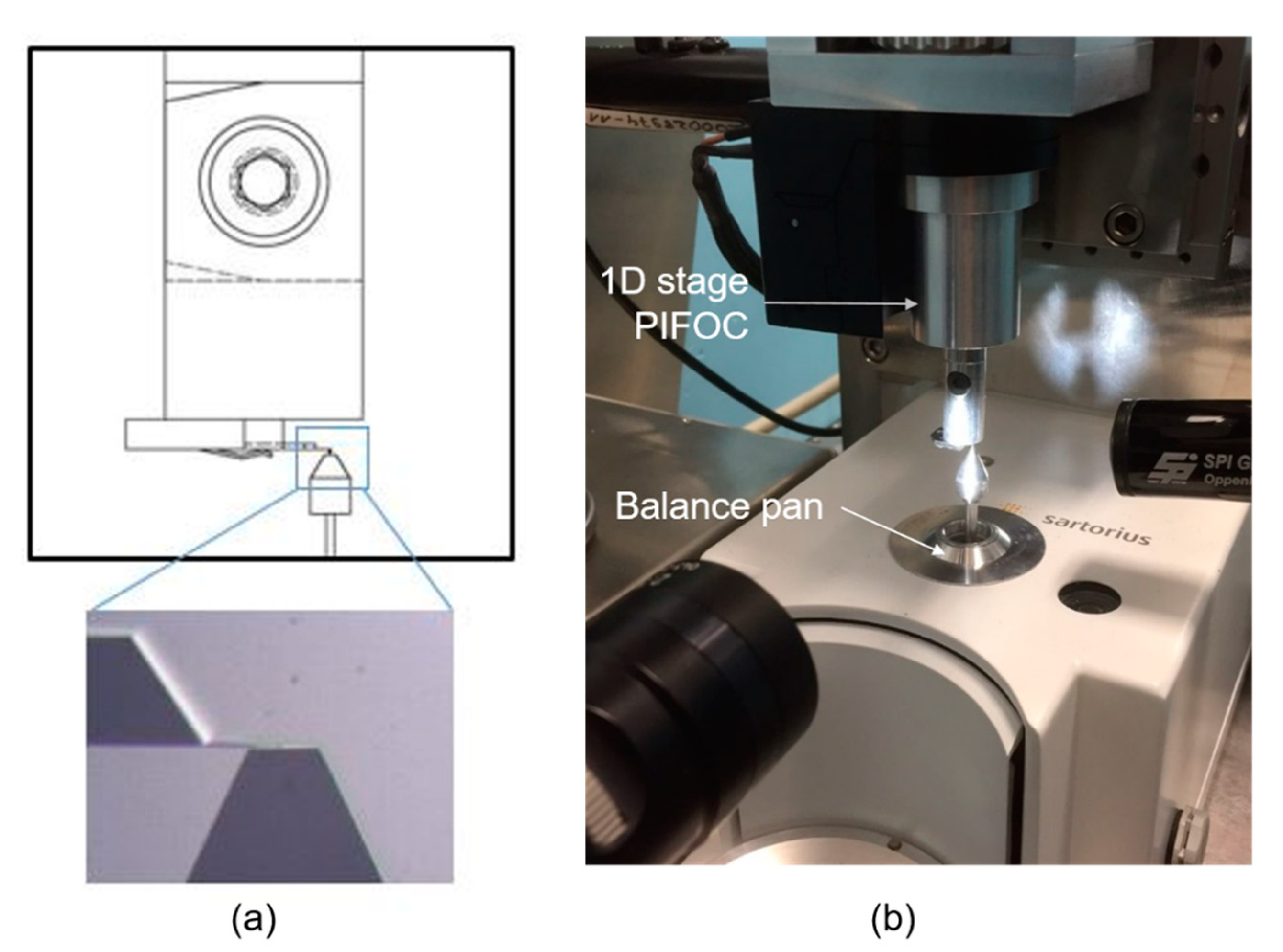
Since a clear knowledge of k₀ is necessary for precise determination of F′ (using Equation (16)), stiffness calibration was exemplarily performed with some selected cantilevers. This was conducted using the force/balance method [31]. Here, a nano-force measuring setup comprising of a one dimensional (1D) translational positioning stage (P-726 PIFOC, from Physik Instrumente (PI) GmbH & Co. KG, Karlsruhe, Germany: resolution 1 nm, uncertainty 10 nm) was used to precisely move the cantilever, as well as a commercially available compensation balance (Sartorius SE-2 micro-balance: resolution 1 nN, reproducibility 2.5 nN, linearity deviation 9 nN, uncertainty 0.1 µN) (see Figure 1). The cantilever chip comprising a conical tip at its free end was mounted on the 1D stage, with the tip oriented downwards. A 2-micron-sized sphere (composed of polished ruby) was mounted on the balance pan and then utilized as a probing area.

During stiffness calibration measurement, the cantilever was equidistantly and incrementally moved down in defined steps (~0.1 µm) until it touched the ruby sphere and some micrometers further in order to measure the probing curve. Force deflection curves were then measured up to a maximum force of 10.2 µN. The position of the cantilever and the mass of the compensation balance were then simultaneously recorded. In this case, five measurement cycles were performed, each cycle comprising of 20 measurements. The averages and standard deviations from each measurement cycle were then pooled together to determine the mean value and the repeatability (standard uncertainty). If we take into consideration other uncertainty contributions such as temperature drift, humidity, balance/mass comparator and the tip (orientation), an overall (maximum expanded) uncertainty in spring constant calibration of ± 4% (corresponding to about 95% confidence level) was estimated.

Another important pre-calibration process that was performed was to clean up the cantilevers in acetone to remove dust and any other contaminants that would otherwise be on the surface. Moreover, to guarantee and render the sensors re-usable after adsorbing magnetic particles thereon, each cantilever was cleaned by sonicating in acetone for about 3–5 min. Before sonication, a cantilever was mounted on a specially designed metallic holder to mitigate the risk of breakage [32]. Thus, repetitive use of the cantilever sensor was possible.

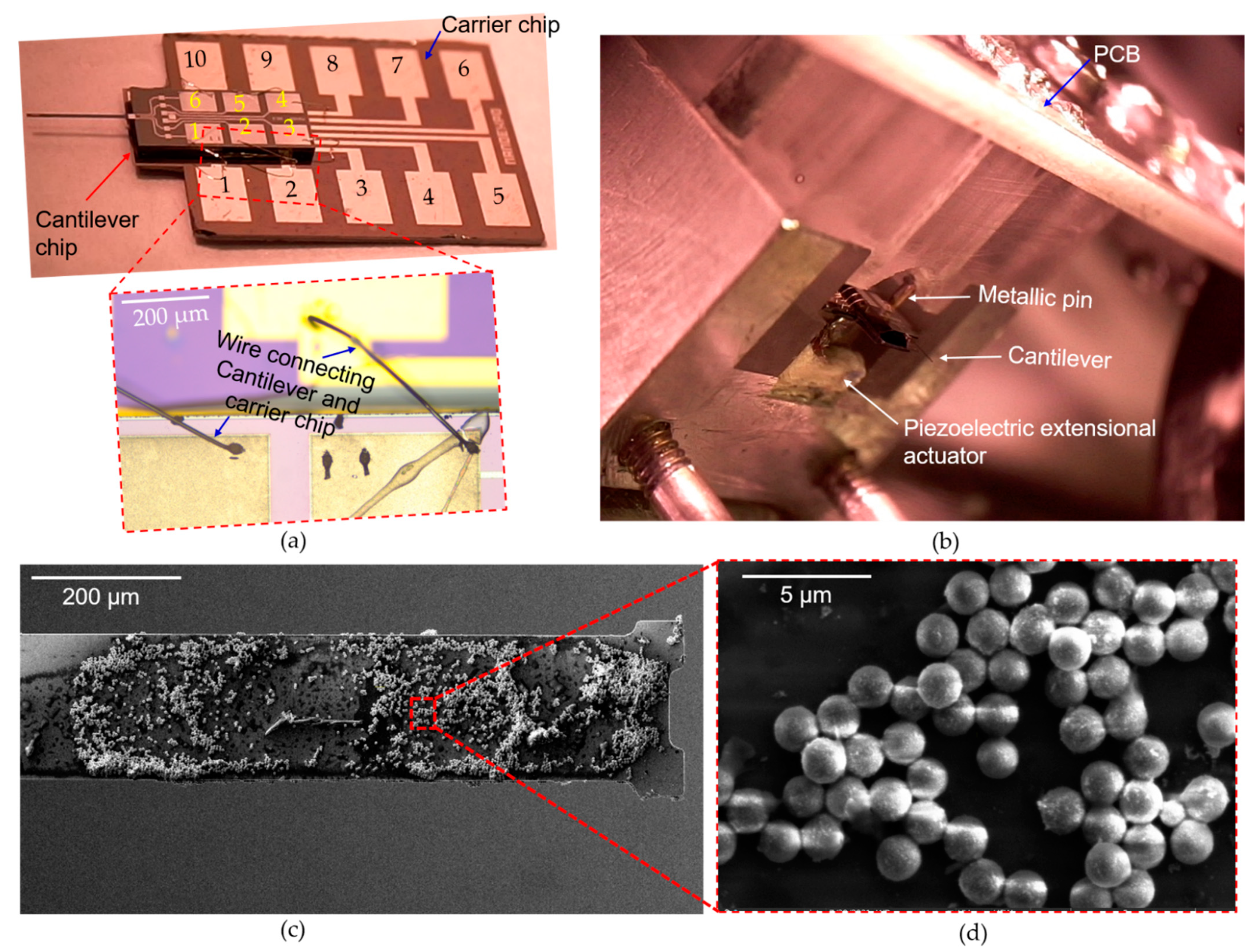
Individual sensor chips were glued onto in-house carrier chips, and their contact pads were electrically connected via wire-bonding (Figure 2a). The prepared chip was then mounted onto a cantilever sensor PCB (fixed on a workbench). Consequently, the contact pads of the carrier chip were contacted through metallic shafts (fixed onto the PCB, see Figure 2b) and then fastened/screwed.

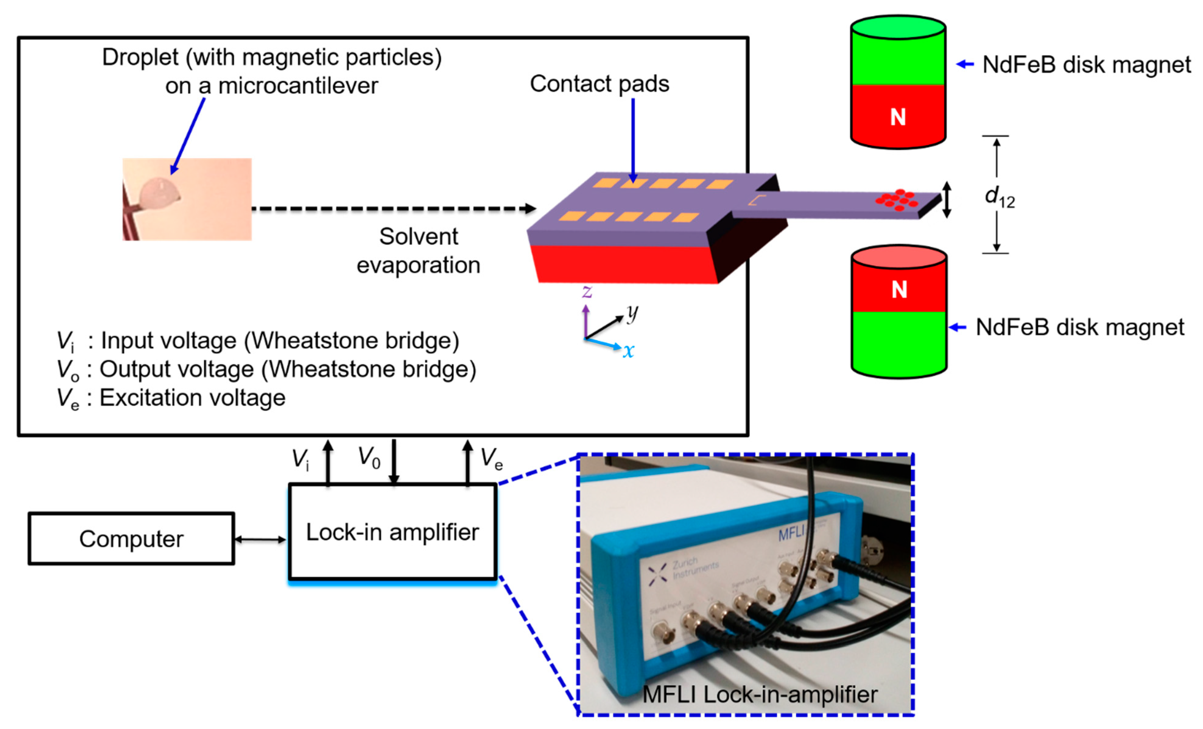
To supply (or obtain) voltage to (or from) the cantilever sensor (Wheatstone bridge), SMA coaxial cables were connected to dedicated SMA connectors (ports) on the cantilever sensor holder PCB. Here, a lock-in amplifier (MFLI, from Zurich Instruments AG, Zurich, Switzerland) was used to supply voltage to both the cantilever sensor (up-to 5 Vdc) and piezo actuator (up-to 10 Vpk). Each cantilever was placed on the piezo actuator (within the cantilever sensor holder PCB), as depicted in Figure 2b.

Subsequently, magnetic particles solution was deposited onto the cantilever sensors. Deposition of MPs solution on the sensor’s surface was performed based on droplet dispensing approach, as discussed in a previous work [33]. In general, a small liquid volume was deposited and solvent vaporized under ambient conditions, leaving behind (on the beam) an adsorbate of MPs. Localized deposition of the MPs was conducted at a point towards the free-end of the sensing beam, aided by a digital camera. The added particle mass Δm proportionately changed the unloaded resonant frequency of the cantilever by Δf as follows [32]:

$$\Delta m=-\frac{2m_0}{f_0}\frac{1}{U^{ 2}{(x}_{\Delta m})}\Delta f$$

(11)

where U(x_Δm) is the dimensionless parameter denoting the mode shape function of the cantilever. The number of particles added on the cantilever sensor was then determined from the ratio of total measured Δm to the mass per particle, m_p.

To realize magnetization of the particles into the direction perpendicular to the cantilever surface prior to their immobilization after solvent evaporation, we dispensed the droplet on the cantilever after positioning it in the field of a permanent magnet as described below. It should be noted that whenever the particles were immobilized after solvent evaporation, Brownian relaxation was suppressed and a constant/remanent magnetization prevailed.

2.1.3. Magnets and Magnet Assembly

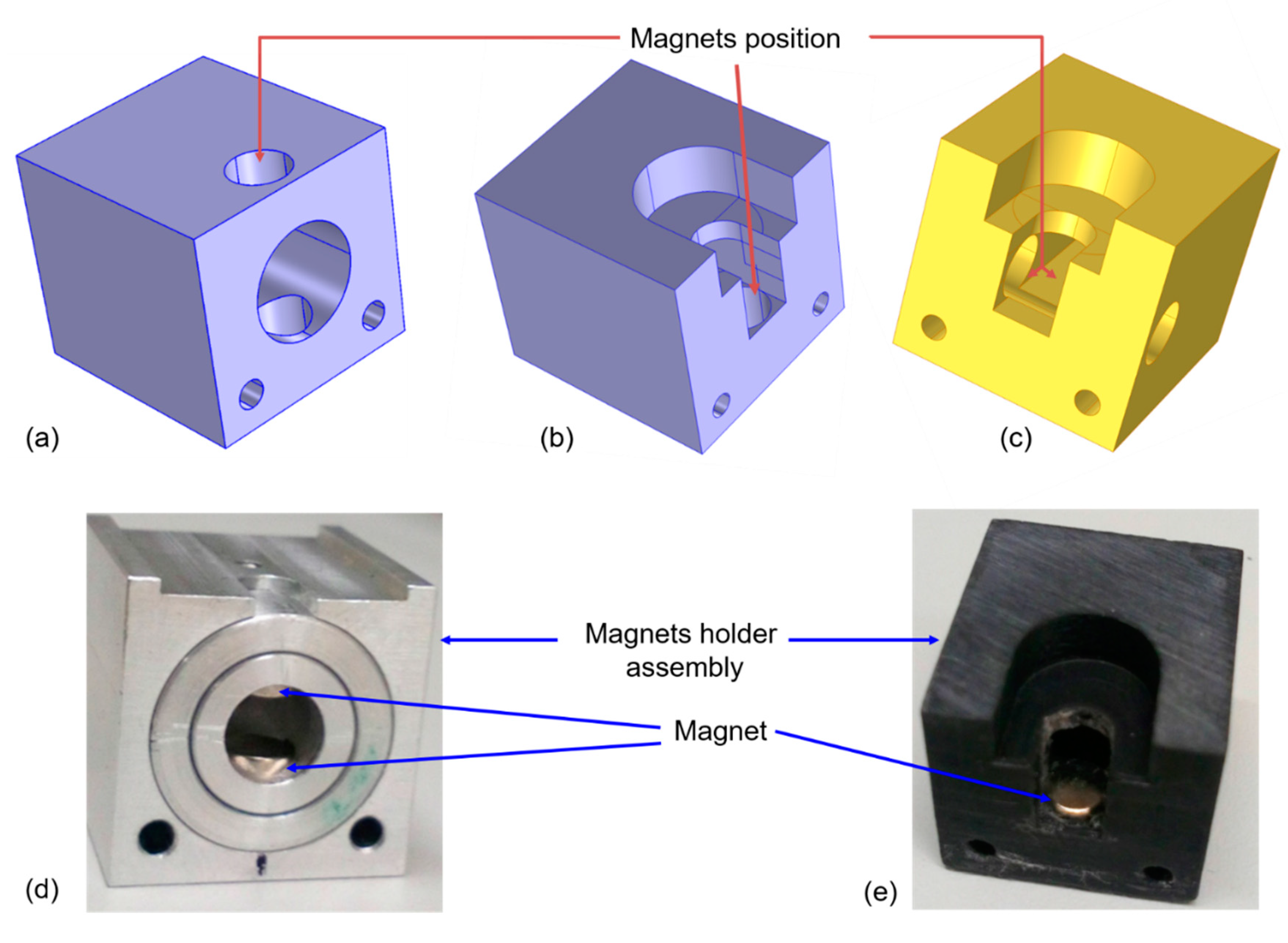
A magnetic field, created by a pair of Neodymium (NdFeB) permanent disk magnets (from Webcraft GmbH, Gottmadingen, Germany) was used to align the magnetic moment of the magnetic particles and to induce a magnetic force gradient in the same direction. The radius r_m and length l_m of these axially magnetized identical NdFeB magnets (type N42) were 5 mm and 3 mm, respectively. Their average residual magnetism and coercive field strength was ~1.31 T and 908 kA/m [34], respectively. These magnets were mounted in the magnets holder assemblies, whose designs and fabricated samples are shown in Figure 3.

2.2. Finite Element Modeling of Second-Derivative Magnetic Field

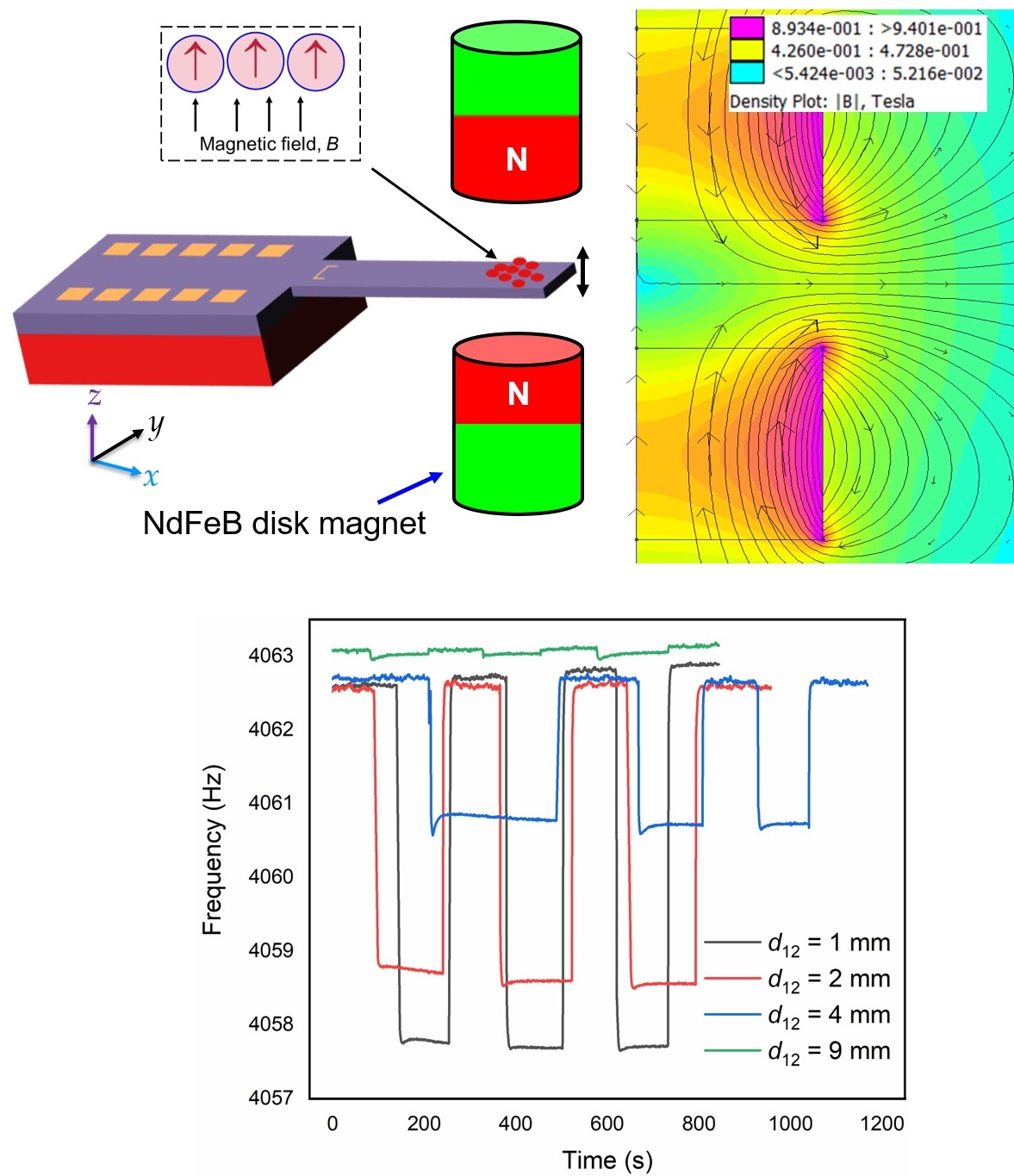
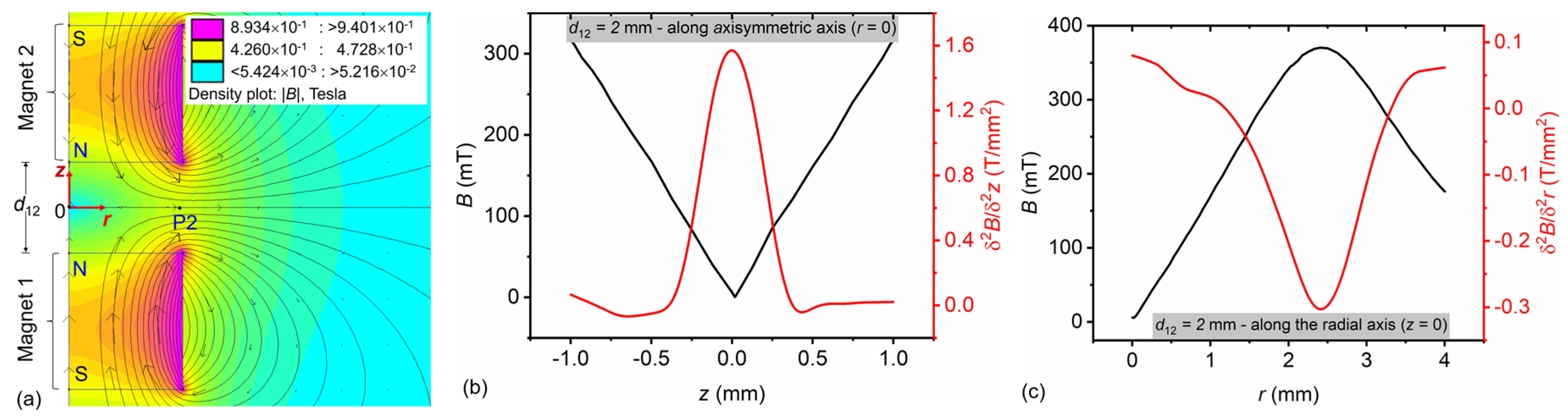
The magnetic force gradient was determined by finite element modeling using the Finite Element Method Magnetics, FEMM v. 4.2 software [35]. To tune the magnetic field B and its second spatial derivative along z (δ²B/δz²), two parameters were considered: the distance between a pair of magnets d₁₂ and the arrangement of the permanent magnets. Here, as depicted in Figure 4a, the two NdFeB permanent magnets were configured with a face-to-face arrangement. These magnets possess axisymmetric magnetization (i.e., with the magnetization direction through the axis of the magnet). The spatial magnetic field distribution generated by the two repelling (opposing) faces of magnets (i.e., north-to-north pole, N–N, or south-to-south pole, S–S) along the z-axis and r-axis is for instance depicted in Figure 4b,c, in which magnets had a spacing of d₁₂ ≈ 2 mm.

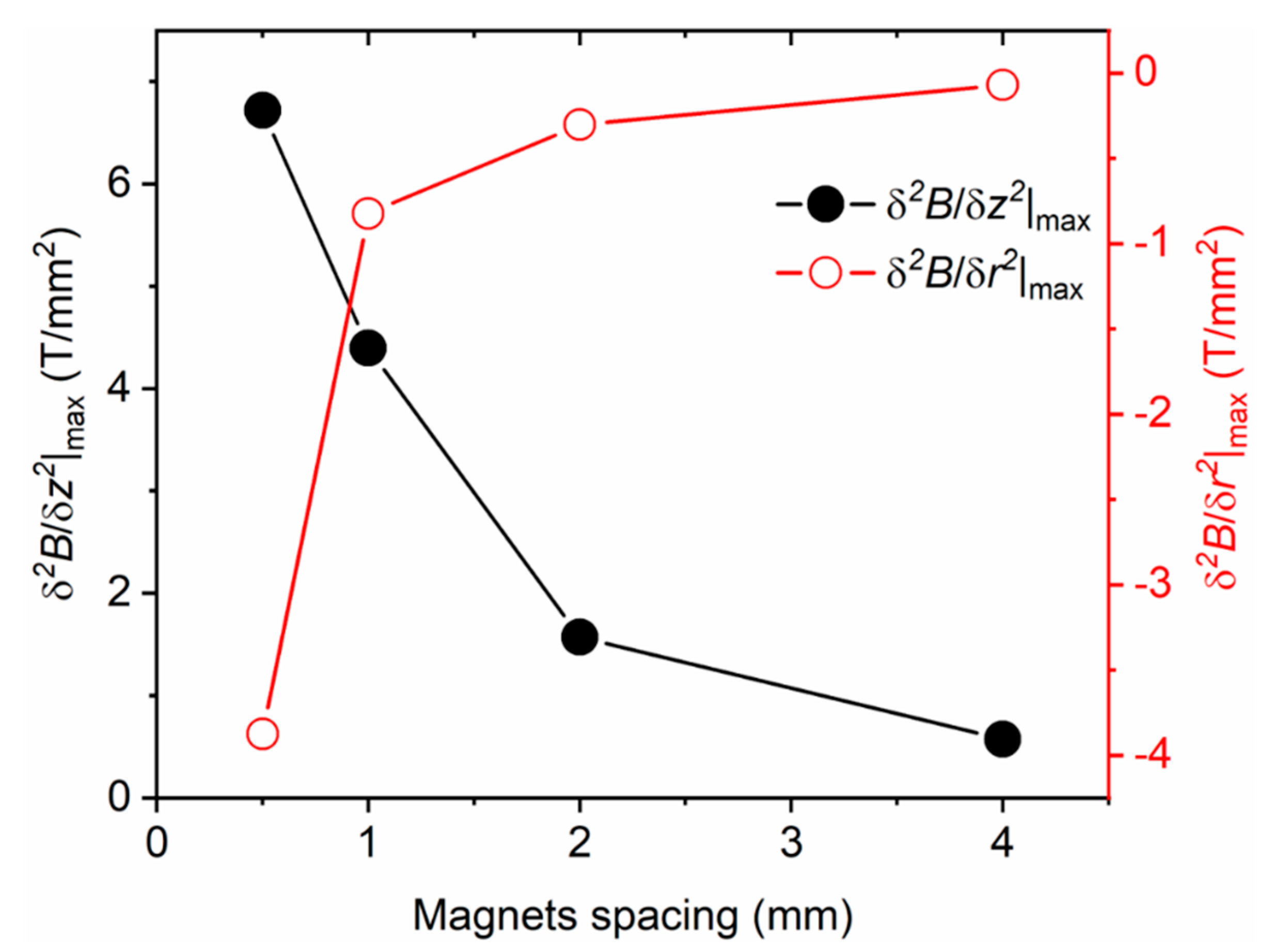
In Figure 5, we show the maximum magnetic induction field (for two identical NdFeB disk magnets in repelling arrangement) vs. magnets–pole spacing, along the axisymmetric (z) and radial (r) axes. With the latter, the indicated maximum induction field was observed nearly at the edge of the magnet (i.e., at r ≈ 2.5 mm). With the former (i.e., Figure 4b) as expected, the zero B-field was observed at the mid-point between the two permanent magnets with opposing faces (N-N or S-S). Usually, B-values would be negative to one side (field lines point in opposite directions) and then the graph was almost a straight line over the entire field of view. However, as depicted in Figure 4a, an absolute value of B (i.e., |B|) was used, leading to a sharp change of slope at z = 0. This was in contrast to Figure 5, where with increasing r the B-field approached a maximum at r ≈ 2.5 mm under a steadily decreasing slope.

For a 2 mm magnets spacing, we found a maximum second derivative of magnetic flux density δ²B/δz²|_max ≈ 1.57 T/mm² along z-axis (cf. red solid line, Figure 4b), whereas along the radial axis the maximum gradient δ²B/δr²|_max ≈ 0.30 T/mm² was much lower (i.e., at point P2, cf. Figure 4a; red solid line, Figure 4c). Therefore, the former condition was adopted for the experiments as subsequently described. Here, the second derivative fields were determined by finite difference approximation of the spatial field distribution along the z and r axis, respectively.

3. Results and Discussion

3.1. Magnetic Force Gradient Sensing

To generate an interaction of the magnetic force gradient induced by the second derivative of the B field with the magnetic particles on the cantilever, pre-magnetization was performed. Hence, the particle-laden droplet (on the cantilever) was deposited and immediately subjected to the magnetizing field prior to complete solvent evaporation. We assumed that through the Brownian relaxation mechanism the particles easy axes rotated in the z-direction (i.e., along the applied field) [36]. To realize this, we used the magnet holder in Figure 3e. This holder assembly gave the possibility to deposit the particles on the cantilever in the form of a water suspension (as a droplet) and then simultaneously align them into the direction perpendicular to the cantilever surface. In essence, this happened prior to the particle immobilization after the solvent evaporation. Under the influence of an external magnetic field (induced by a permanent magnet), it suffices to mention that the dispersion of magnetic particles within the droplet could be biased towards the droplet base (contact line). In this work though, this was inconsequentially assumed since the liquid was evaporated before conducting the measurement. Upon complete evaporation, the particles were adsorbed on the sensing surface (cf. Figure 2c,d).

To detect the cantilever-stiffness-changing effect of the magnetic force gradient, the setup depicted in Figure 6 was employed. This mainly comprised the sensor (cantilever plus attaching particles magnetized in z direction) and a magnetic force gradient (induced also in z direction by two permanent magnets spaced d₁₂ apart). From Figure 5, δ²B/δz²|_max and δ²B/δr²|_max varied with respect to the distance d₁₂ between the poles of the two magnets. Thus, as deducible from Equation (5), to generate a sufficiently large magnetic force gradient F′, d₁₂ had to be set as small as possible. Moreover, by subjecting the immobilized particles to a magnetizing field (in z direction) during the cantilever frequency response measurement, a further alignment (through the Néel relaxation mechanism, i.e., the rotation/alignment of the particle’s magnetic moment inside the magnetic core with the applied field against an energy barrier without interacting with the particle’s surrounding [16]) could be assumed. This was favorably due to the fact that both magnetic particles were composed of small crystallites (less than 10 nm in size).

In detecting the magnetic force gradient F′(z₀) = ∂F/∂z|_z0, a cantilever should be sinusoidally driven around its equilibrium position by a force F(z₀) along the z axis (Figure 6) in accordance to the equation of motion for a lumped element oscillator [37]:

$$m_0\frac{{\partial }^{2}z}{\partial t^2}+\gamma \frac{\partial z}{\partial t}+(k_0-F^{\prime }\left(z_0\right))z=F\left(z_0\right)$$

(12)

where γ denote the damping coefficient, and the term k₀ − F′(z₀) is equivalent to the effective spring constant of the cantilever. Based on Equation (12), it is evidently clear that the magnetic force gradient F’ acted to soften (reduce) or harden (increase) the spring constant. Consequently, this served to modulate and shift the cantilever resonance frequency Δf’. Utilizing Equations (5) and (12) yielded Equation (13). If we assume F′/k₀ to be << 1, then using the first order Taylor series expansion, Equation (13) reduces to Equation (14). By substituting the angular frequency ω with the ordinary frequency f, we obtained the resonant frequency shift Δf’ due to the influence of the magnetic force gradient F′ as delineated in Equation (15).

$$\omega =\sqrt{\frac{k_0-F^{\prime }}{m}}={\omega }_0\sqrt{1-\frac{F^{\prime }}{k_0}}$$

(13)

$$\omega \approx {\omega }_0\left(1-\frac{F^{\prime }}{2k_0}\right)$$

(14)

$$\mathsf{\Delta }{f}^{\prime }\approx -\frac{f_0}{2k_0}{F}^{\prime }$$

(15)

Thus, by rearranging Equation (15) we obtained:

$$F^{\prime }\approx -\frac{2k_0}{f_0}\mathsf{\Delta }{f}^{\prime }$$

(16)

Under ideal measurement conditions (e.g., free of dust and contaminants), the total mass of the cantilever (i.e., m₀ + ∆m) does not change upon exposure to the external magnetic force field gradient. Thus, the attached magnetic particles mass ∆m was assumed to be invariant.

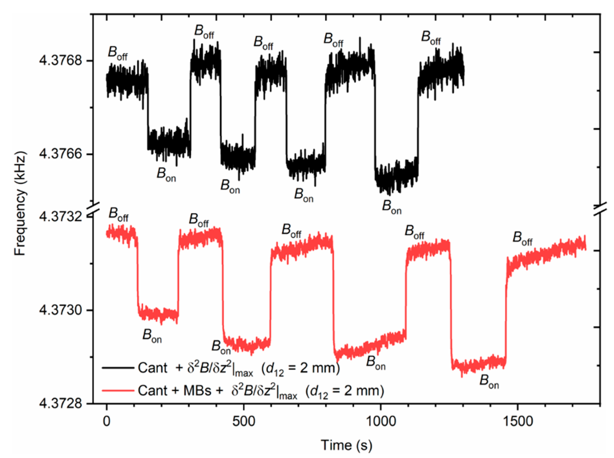
In Equations (15) and (16), Δf’ is the effective typical resonant frequency difference between a cantilever (containing magnetic particles), within and without external magnetic fields exposure. To determine it, blank measurements were performed beforehand, as depicted with the black line graph in Figure 7. Here, a change in the resonant frequency of an unloaded clean cantilever was unexpectedly observed upon exposure to an external magnetic force field. It should be noted that the silicon-based cantilever contains electrical/metallic connection lines which were not shielded from the external magnetic field. Thus, if a current was induced in the electrical conductors it would produce thermal energy (Joule heating). Upon a rise in temperature, the Young’s modulus of silicon and stiffness k₀ will decrease. Furthermore, we suppose that the cantilever may experience stress, e.g., by a bimorph effect due the stack of materials of different thermal expansion coefficients built in the cantilever, that consequently alter the fundamental resonant frequency of the vibrating system.

In Figure 7, B_on and B_off represent the manual switch on and off of the magnetic force field, respectively. It should be noted that the average frequency difference between the B_off states corresponded to the resonant frequency shift Δf due to the added mass Δm = 8.22 ± 0.54 ng (N_p = 2050 ± 135). Furthermore, it is worth noting that there was no systematic phase shift between the unloaded and loaded cantilever excitation conditions. Thus, to determine the change in resonant frequency (Δf’) due to the externally induced magnetic field on the magnetic moment of particles, the average resonant frequency due to B_on state was subtracted from that of B_off.

To determine F′ using Equation (16), a known (calibrated) value of k₀ and the frequency shift Δf’ were required. For instance, in Figure 7, Δf’ ≈ −22 ± 12 mHz (i.e., the effective frequency difference obtained from a cantilever (CAN30-1-2) with and without magnetic polystyrene particles under a magnetic force field condition comprising of two permanent magnets placed 2 mm apart). This cantilever’s calibrated stiffness k₀ was 4.46 ± 0.09 N/m. By substituting k₀ and Δf’ into Equation (16), we obtained a magnetic force gradient F′ ≈ 44 ± 24 µN/m, which was considered significant since it was much larger than F′_min = 10 ± 2 µN/m.

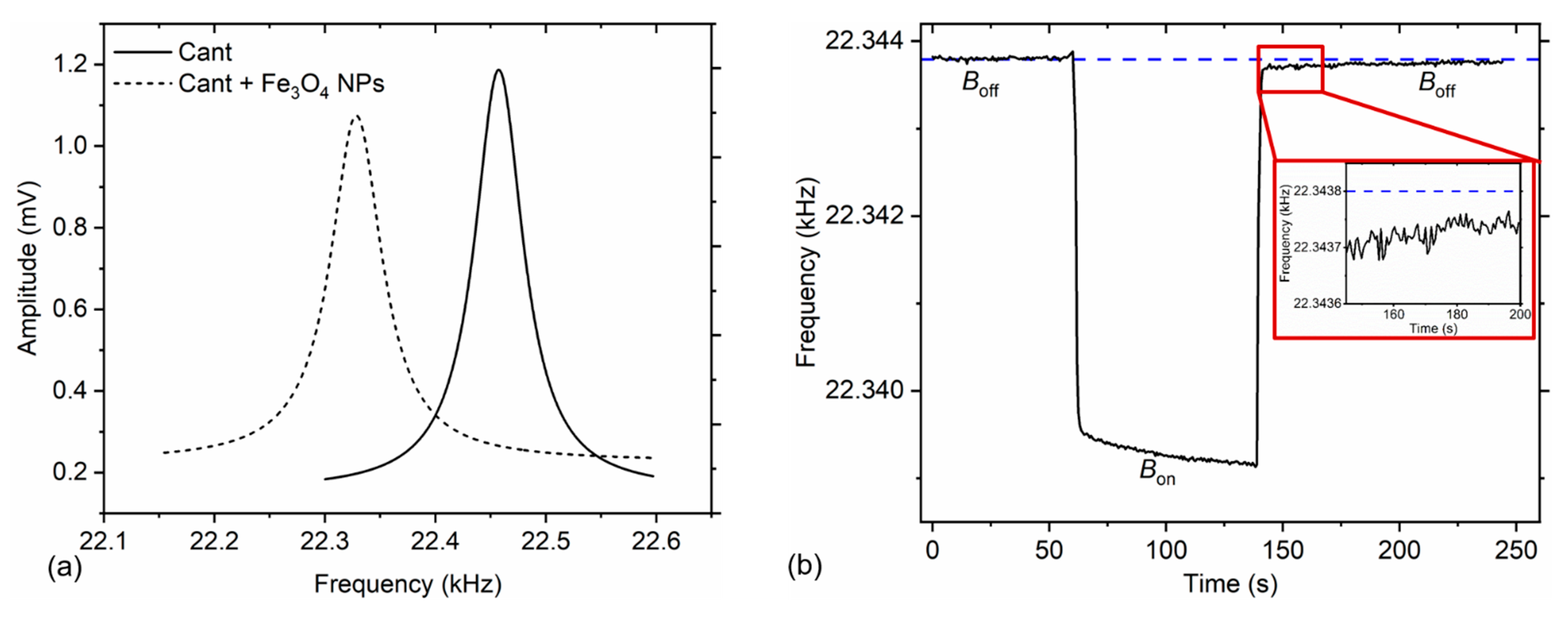
A much clearer trend was observed upon the attaching iron oxide NPs on the cantilever (→ frequency shift by added particles mass, Figure 8a) and subjecting it to the magnetic force gradient under the same conditions as above (Figure 8b). With these particles, Δf’ and F′ were about −4.1 ± 0.2 Hz and 4.53 ± 0.94 mN/m, respectively. Since the stiffness of this type of cantilever (k₀ ≈ 12.5 ± 0.8 N/m, CAN15-3-2, Equation (5)) was larger than that of CAN30-1-2 (cf. Figure 7), its sensitivity to the external magnetic force field was lower. However, as depicted in Figure 8b, the induced frequency shift was much larger compared to Figure 7. This was mainly attributed to the much larger number of attached particles (N_p = (254 ± 21) × 10³ vs. 2050 ± 135 in case of the magnetic polystyrene beads). Consequently, this yielded an almost one-order of magnitude higher total magnetic moment of the plain iron oxide particles compared to magnetic polystyrene beads (even though their magnetic moment per particle was more than one order of magnitude lower, cf. Table 1). Nonetheless, a slight continuous change in frequency was visible in the B_on state on Figure 8b which is supposedly due to temperature change effect on the magnetic particle magnetization or the cantilever (whose increase led to a decrease in cantilever stiffness).

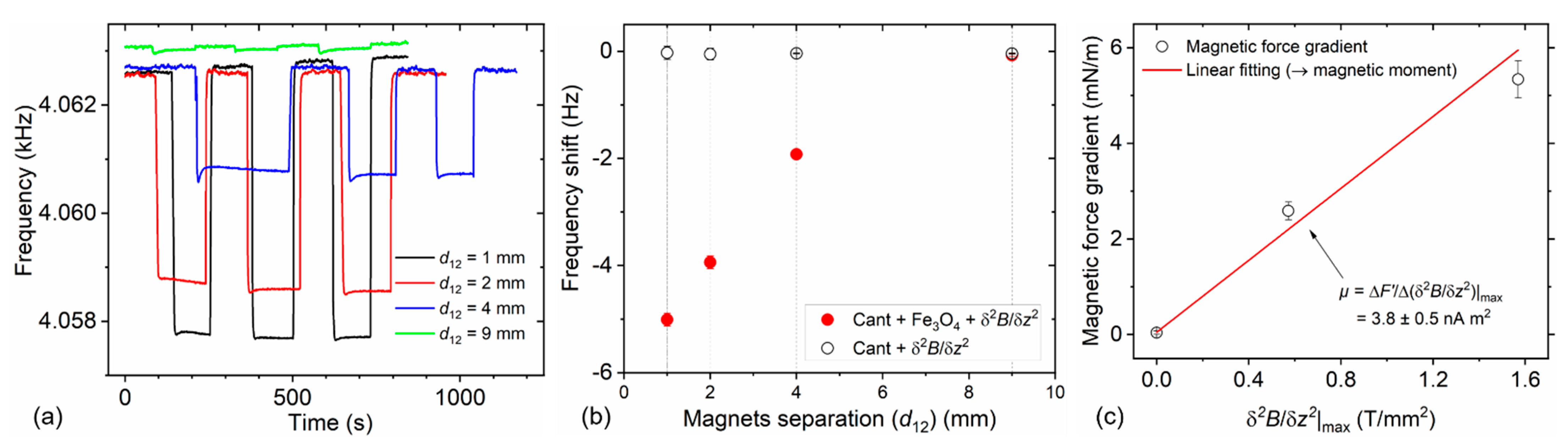
To determine the frequency response of a cantilever sensor (with 230 ± 20 ng of 250 nm-sized iron oxide particles, S84/CAN30-1-2) under different magnetic force gradients, the distance between a pair of magnets was sequentially reduced in steps (see Figure 9a). In this condition, the position of the cantilever was fixed at a point nearly at the midpoint of the magnets, while the magnets’ spacing (d₁₂) was varied from about 9 mm (green line) to 4 mm (blue line), 2 mm (red line) and 1 mm. As expected, in the magnetic force gradient environment, the resonant frequency changes on the bare cantilever tend to zero (nearly negligible, open red circles in Figure 9b), while for the cantilever loaded with magnetic particles it increased with decrease in the distance between the two identical magnets (see full red circles in Figure 9b). Consequently, in Figure 9c we show the magnetic force gradient (derived from the effective frequency shifts in Figure 9b using Equation (10)) against the corresponding second-derivative magnetic-induction gradient. According to Equation (7), the resultant slope of the linear fitting in Figure 9c was equivalent to the total magnetic moment (μ = 3.8 ± 0.5 nA m²) in the test sample.

In

Table 3. Magnetic force gradient under 2 mm magnets spacing (with δ²B/δz²|_max ≈ 1.57 T/mm²) from assorted cantilever sensors with different resonance attributes and attached particle masses.

Cantilever ID/Type (MPs)	f0 (Hz)	Δf0 (Hz)	Δm × 10−9 (g)	k0 (N/m)	Δf0′ (Hz)	F’(z) (mN/m)
S97/CAN30-1-2 (Micromer)	4667.75 ± 0.02	−1.87 ± 0.04	3.79 ± 0.26	3.61 ± 0.24	−0.01 ± 0.01	0.02 ± 0.01
S80/CAN30-1-2 (Micromer)	4377.08 ± 0.01	−3.72 ± 0.02	8.22 ± 0.54	4.46 ± 0.09 †	−0.02 ± 0.01	0.04 ± 0.02
				3.17 ± 0.13		0.03 ± 0.02
				2.45 ± 0.20 ‡		0.02 ± 0.01
S95/CAN30-1-2 (Micromer)	4611.90 ± 0.05	−10.51 ± 0.05	23.2 ± 1.5	3.52 ± 0.23	−0.11 ± 0.02	0.17 ± 0.04
S89/CAN15-3-2 (Fe3O4)	21,448.63 ± 0.06	−18.50 ± 0.06	1.63 ± 0.11	11.43 ± 0.75	−0.08 ± 0.03	0.09 ± 0.03
S88/CAN15-3-2 (Fe3O4)	22,465.52 ± 0.12	−131.67 ± 0.13	11.06 ± 0.73	12.53 ± 0.82	−4.06 ± 0.20	4.53 ± 0.94
S84/CAN30-1-2 (Fe3O4)	4148.50 ± 0.01	−84.90 ± 0.01	230 ± 20	2.85 ± 0.19	−3.89 ± 0.12	5.34 ± 0.39

^† from load-deflection calibration curves. ^‡ from Equation (4).

, the derived magnetic force gradient observed with a varying attached particles mass (numbers) on various assorted piezoresistive cantilevers is presented. For sensors with nearly the same k₀ and comparable f₀, an increase in the particle mass resulted in a corresponding increment in the magnetic force gradient. It is also evidently clear that the force gradient varied with the particles type on the beam. In which case, for cantilevers with comparable masses (such as on sensors S97 and S89), the frequency response due to Fe₃O₄ NPs was found to be much greater compared to the microbeads (magnetic polystyrene particles), which was attributed to the much larger particle numbers. Moreover, taking the S80/CAN30-1-2 cantilever (Table 3) into consideration, the calibrated cantilever stiffness was found to differ with the calculated values by about 45% (Equation (4)) and 28% (Equation (5)), which is generally expected mainly due to an uncertainty of the cantilever thickness related to the fabrication tolerances. Replication of these variances was obviously expected on their respective calculated magnetic force gradients. Consequently, the calibrated stiffness has a lower uncertainty compared to calculated values. With calibration, it should be noted that the measurements were performed under stable ambient conditions, and the repeatability (the major source of uncertainty) was small, ~6 mN/m.

3.2. Magnetic Moment Determination

The nominal magnetic moment calculated for each magnetic particle sample (Table 1) assumed that all the particles were 100% polarized along the easy axis. For a known particle mass, the total nominal magnetic moment μ on the cantilever could be determined based on Equation (10). Considering a mass-induced frequency change Δf = −3.72 ± 0.02 Hz due to the added magnetic polystyrene particles (Δm = 8.22 ± 0.54 ng; cf. Table 3) yielded a total nominal magnetic moment of 28 ± 15 pA m². For iron oxide NPs on a CAN15-3-2 cantilever with Δf = −131.67 ± 0.13 Hz (→N_p = (254 ± 21) × 10³), μ = 2.9 ± 0.6 nA m² (Equation (7)).

Using the magnet arrangement with d₁₂ ≈ 2 mm (→ δ²B/δz²|_max ≈ 1.57 T/mm²), the corresponding magnetic moment per particle was determined from our measurements using Equation (7) as indicated in

Table 4. Magnetic force gradient (under 2 mm magnets spacing) and derived magnetic moment per magnetic particle.

Cantilever ID/Type (MPs)	F’(z0) (mN/m)	Σµ (pA m2)	Np	µ per MP (fA m2)
				by Cantilever♀	Nominal	by SQUID
S97/CAN30-1-2 (Micromer)	0.02 ± 0.01	10 ± 6	945 ± 65	11 ± 7	33	116.6 ± 0.5 † 120.8 ± 0.4 ‡
S80/CAN30-1-2 (Micromer)	0.04 ± 0.02	28 ± 15	2050 ± 135	14 ± 8
S95/CAN30-1-2 (Micromer)	0.17 ± 0.04	110 ± 21	5792 ± 382	19 ± 4
S88/CAN15-3-2 (Fe3O4)	4.53 ± 0.94	2887 ± 602	(254 ± 21) × 103	11 ± 3	2	2.379 ± 0.001 † 2.571 ± 0.013 ‡
S89/CAN15-3-2 (Fe3O4)	0.09 ± 0.03	55 ± 21	(37 ± 3) × 103	1.5 ± 0.8
S84/CAN30-1-2 (Fe3O4)	5.34 ± 0.39	3402 ± 247	(4506 ± 372) × 103	0.75 ± 0.08
		3761 ± 526 *		0.83 ± 0.1

* From the slope of F’ vs. δ²B/δz² in Figure 9c, based on Equation (7); ^♀ In determining stiffness k₀, the full cantilever length L was used here. However, since particles were not concentrated at the free end of the cantilever a smaller length (corresponding to the average position of the particles along L) would yield a larger stiffness k_eff. Consequently, a larger magnetic moment which ultimately depicts a better agreement with the nominal value would be expected; ^† at 800 kA/m (= 1 T); ^‡ at 1592 kA/m (= 2 T).

. In case of the micromer beads, the average resultant magnetic moment per particle was about 15 ± 10 fA m² (Table 4) compared to the 33 fA m² nominal value (see Table 1). For Fe₃O₄ particles, an average magnetic moment per particle of about 1.2 ± 0.8 fA m² was achieved (from S89 and S84), which was also slightly lower than the nominal magnetic moment (2 fA m²). Unlike the other sensors, S88 yielded a much larger magnetic moment, which we consider as an outlier. Of all the used cantilevers, S88/CAN15-3-2 was evidently the stiffest. Nevertheless, the observed large deviation from nominal magnetic moment could probably arise from sensor positioning error within the second derivative B field, and variance in particle size distribution.

Furthermore, it was also assumed that the magnetic moments in the MP were 100% aligned perpendicular to the cantilever surface (along the cantilever deflection) along the easy axis. This was essentially important for the quantitative determination of magnetic moment per particle µ_p. At the center position between the magnets, the magnetizing field was usually zero; thus, we could not expect a supporting (dynamic) alignment and only the pre-aligned moments contributed to the responses.

To compare and validate the above results, static magnetic moments of the magnetic particles were exemplarily measured using a SQUID-based magnetometer (MPMS-3, from Quantum Design GmbH, Darmstadt, Germany [38,39]), as depicted in Figure 10. To perform these measurements, a 15 µL stock solution of each magnetic particles sample was placed on an in-house designed liquid sample holder. It should be noted that the concentration of the stock solutions was 5.5 × 10⁹ MPs per mL (micromer) and 5.7 × 10¹¹ MPs per mL (iron oxide particles) [23,24]. Thus, a test solution of 0.015 mL corresponds to ~8.25 × 10⁷ MPs (micromer) and 8.55 × 10⁹ MPs (Fe₃O₄). The volume of magnetite for each magnetite polystyrene and iron oxide particles was determined to be 0.15 µm³ and 0.008 µm³, respectively (Table 1). Therefore, the corresponding magnetite total volume (and mass) in the 15 µL test sample for micromer beads and Fe₃O₄ NPs was 0.01 µL (65 µg) and 0.07 µL (373 µg), respectively.

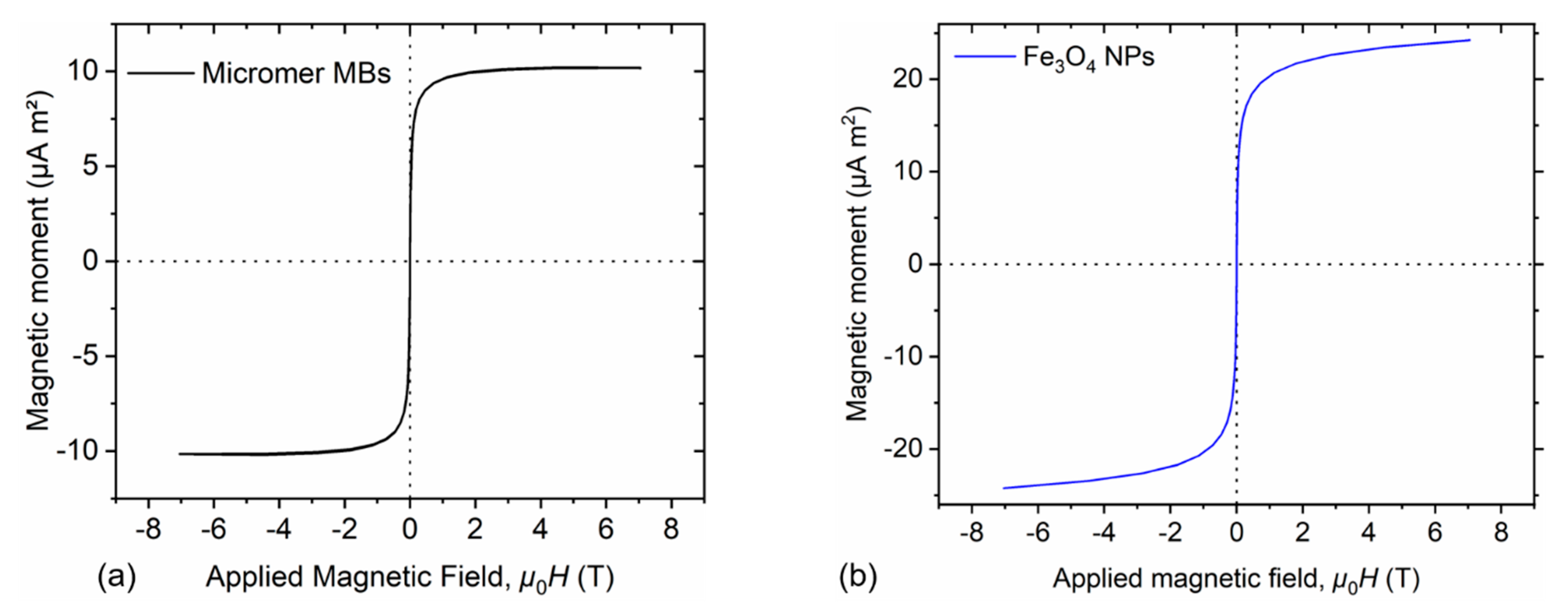
At zero field, the magnetic moment of a particle was nearly zero, or tends thereto (see Figure 10). Moreover, as expected, by increasing the magnitude of the magnetizing field, the magnetic moment concomitantly increased and eventually saturated. It should be noted that in our SQUID measurements, particle suspensions were used and the observed phenomenon (Figure 10) would connotate the superparamagnetic behavior of these particular type of particles. Thus, at the saturating magnetizing field, we could use a corresponding magnetic moment and the total volume of magnetite to determine saturation magnetization M_s (i.e., $M_{\mathrm{s}}=\frac{{\mu }_{\mathrm{p}}}{V_{\mathrm{Fe}3\mathrm{O}4}}$). Consequently, it is possible to determine the mass magnetization M_m,s from the ratio of M_s to the density of magnetite ρ_Fe3O4. For the microbeads (micromer MPs), the magnetic moment saturated at ~9.97 ± 0.03 µA m² (at a magnetizing field H = 1592 kA/m). With Fe₃O₄ NPs, a total magnetic moment of ~21.98 ± 0.11 µA m² was obtained (at H = 1592 kA/m). From Figure 10, the corresponding total magnetic moment at H = 800 kA/m was 20.34 ± 0.01 μA m² (iron oxide plain NPs) and 9.62 ± 0.04 μA m² (magnetic polystyrene particles).

To obtain magnetic moment per particle from SQUID measurements, it’s necessary to divide the total magnetic moment with the total number of magnetic particles in the test sample. Microbead (micromer) and nanobead (Fe₃O₄) yielded 116.6 ± 0.5 fA m² and 2.379 ± 0.001 fA m², respectively, per particle. Obviously, the obtained moment for the microbeads was much greater than both the nominal value (by factor of ~3.5) and the cantilever-based determined moment (Table 4). It should be noted that with SQUID-based measurements, the number of particles in the test samples was estimated from the volume fraction. The observed discrepancies would probably arise from insufficient knowledge of the particle number in the test sample, e.g., homogeneity in particle concentration as well as pipetting errors (volume sampling). In a previous work [39], the possibility of interaction was also observed to affect the effective magnetic moment of the multi-core particle. We also further suppose that a change in polarization over time might affect the measured values. Unlike cantilever-based samples where diluted particle solutions were employed, SQUID-based samples were taken from stock solutions, which is highly concentrated; hence, particles agglomeration was much more probable here.

Unlike SQUID, the determination of the particle number (from the added mass) in the cantilever-based resonance balance approach was much more precise. Moreover, a much smaller liquid sample (pico-sized droplet) could be deposited on the cantilever sensor. In principle, magnetic nanoparticles dynamically reacted to a change in external magnetic field. In order to show their superparamagnetic behavior, here, magnetization measurements could also be performed as the solvent evaporates. Since the evaporation process was rather fast for a small droplet, faster measurements were highly desirable. To effectively facilitate this, a replacement of the manual switching on and off of the field with a much more precise control mechanism involving an electromagnets setup was intended. Moreover, since this measurement system/approach is quite promising, it can also be flexibly adapted for localized particle detection in mapping (magnetic particle mapping [40]).

4. Conclusions

Here, we have presented a resonant-based measurement approach for determining both magnetic particles’ mass m and the magnetic moment µ. With mass determination, an external magnetic force field was negated. Thus, MEMS cantilever-based cantilever sensors containing particles of interest were excited and the induced proportionate changes in resonant frequency (in fundamental mode) were determined. Given the knowledge of the added mass, the particle number concentration of the test samples on the cantilever was evaluated. To obtain µ, a clear knowledge of magnetic force gradient F’ and second derivative magnetic field δ²B/δz² was necessary. The latter was determined from the linear field gradient produced from a magnetic arrangement between two opposing faces of permanent magnets (N–N, or S–S) through FEMM simulation, whereas the former was established from the measured resonant frequency shift Δf’ under an externally induced magnetic gradient field. Using plain iron oxide nanoparticles (250 nm) and magnetic polystyrene beads (2 µm), we obtained a magnetic moment per particle of ~ 1.2 ± 0.8 fA m² and 15 ± 10 fA m² compared to 2 fA m² and 33 fA m² nominal values, respectively. The range of SNR (µ/µ_min) obtainable from the present sensing system was nearly 0.8 to 57. To enhance sensitivity, an ultrathin cantilever design (L × w × h = 2000 × 50 × 5 µm³) based on silicon-on-insulator (SOI)-based MEMS technology was envisaged. This sensor had a much smaller stiffness k₀ ≈ 0.025 N/m and could yield µ_min = 36 fA m² and m_min = 0.62 pg. An array of cantilevers with different spring constants k₀ (or functionalization) could also be considered to further improve the effective sensing response of the cantilever sensor to the magnetic moment. To mitigate the influence of ambient temperature on the results, measurements could also be conducted under controlled environmental conditions.

References

- Mohammed, L.; Gomaa, H.G.; Ragab, D.; Zhu, J. Magnetic nanoparticles for environmental and biomedical applications: A review. Particuology 2017, 30, 1–14. [Google Scholar] [CrossRef]
- Horák, D.; Babic, M.; Macková, H.; Benes, M.J. Preparation and properties of magnetic nano- and microsized particles for biological and environmental separations. J. Sep. Sci. 2007, 30, 1751–1772. [Google Scholar] [CrossRef]
- Schaller, V.; Kräling, U.; Rusu, C.; Petersson, K.; Wipenmyr, J.; Krozer, A.; Wahnström, G.; Sanz-Velasco, A.; Enoksson, P.; Johansson, C. Motion of nanometer sized magnetic particles in a magnetic field gradient. J. Appl. Phys. 2008, 104, 93918. [Google Scholar] [CrossRef]
- Ruffert, C. Magnetic Bead-Magic Bullet. Micromachines 2016, 7, 21. [Google Scholar] [CrossRef] [Green Version]
- Wang, Z.; Wang, L.; Brown, S.I.; Frank, T.G.; Cuschieri, A. Ferromagnetization of target tissues by interstitial injection of ferrofluid: Formulation and evidence of efficacy for magnetic retraction. IEEE Trans. Biomed. Eng. 2009, 56, 2244–2252. [Google Scholar] [CrossRef]
- Pankhurst, Q.A.; Connolly, J.; Jones, S.K.; Dobson, J. Applications of magnetic nanoparticles in biomedicine. J. Phys. D Appl. Phys. 2003, 36, R167–R181. [Google Scholar] [CrossRef] [Green Version]
- Philippova, O.; Barabanova, A.; Molchanov, V.; Khokhlov, A. Magnetic polymer beads: Recent trends and developments in synthetic design and applications. Eur. Polym. J. 2011, 47, 542–559. [Google Scholar] [CrossRef] [Green Version]
- Yoon, T.-J.; Kim, J.S.; Kim, B.G.; Yu, K.N.; Cho, M.-H.; Lee, J.-K. Multifunctional nanoparticles possessing a “magnetic motor effect” for drug or gene delivery. Angew. Chem. Int. Engl. 2005, 44, 1068–1071. [Google Scholar] [CrossRef] [PubMed]
- Williams, H.M. The application of magnetic nanoparticles in the treatment and monitoring of cancer and infectious diseases. Biosci. Horiz. Int. J. Stud. Res. 2017, 10, 257. [Google Scholar] [CrossRef] [Green Version]
- Alexiou, C.; Diehl, D.; Henninger, P.; Iro, H.; Rockelein, R.; Schmidt, W.; Weber, H. A High Field Gradient Magnet for Magnetic Drug Targeting. IEEE Trans. Appl. Supercond. 2006, 16, 1527–1530. [Google Scholar] [CrossRef]
- Tenório-Neto, E.T.; Jamshaid, T.; Eissa, M.; Kunita, M.H.; Zine, N.; Agusti, G.; Fessi, H.; El-Salhi, A.E.; Elaissari, A. TGA and magnetization measurements for determination of composition and polymer conversion of magnetic hybrid particles. Polym. Adv. Technol. 2015, 26, 1199–1208. [Google Scholar] [CrossRef]
- Liu, C.; Stakenborg, T.; Peeters, S.; Lagae, L. Cell manipulation with magnetic particles toward microfluidic cytometry. J. Appl. Phys. 2009, 105, 102014. [Google Scholar] [CrossRef]
- Aziz, T.; Masum, S.; Qadir, M.; Gafur, A.; Huq, D. Physicochemical Characterization of Iron Oxide Nanoparticle Coated with Chitosan for Biomedical Application. IRJPAC 2016, 11, 1–9. [Google Scholar] [CrossRef]
- Moreland, J.; Nakashima, Y.; Alldredge, J.W.; Zabow, G. Novel methods for in situ characterization of individual micro- and nanoscale magnetic particles. MRS Bull. 2013, 38, 933–937. [Google Scholar] [CrossRef] [Green Version]
- Alldredge, J.W.; Moreland, J. Magnetic particle imaging with a cantilever detector. J. Appl. Phys. 2012, 112, 23905. [Google Scholar] [CrossRef]
- Draack, S.; Viereck, T.; Nording, F.; Janssen, K.-J.; Schilling, M.; Ludwig, F. Determination of dominating relaxation mechanisms from temperature-dependent Magnetic Particle Spectroscopy measurements. J. Magn. Magn. Mater. 2019, 474, 570–573. [Google Scholar] [CrossRef]
- Draack, S.; Lucht, N.; Remmer, H.; Martens, M.; Fischer, B.; Schilling, M.; Ludwig, F.; Viereck, T. Multiparametric Magnetic Particle Spectroscopy of CoFe 2 O 4 Nanoparticles in Viscous Media. J. Phys. Chem. C 2019, 123, 6787–6801. [Google Scholar] [CrossRef]
- van de Loosdrecht, M.M.; Draack, S.; Waanders, S.; Schlief, J.G.L.; Krooshoop, H.J.G.; Viereck, T.; Ludwig, F.; Ten Haken, B. A novel characterization technique for superparamagnetic iron oxide nanoparticles: The superparamagnetic quantifier, compared with magnetic particle spectroscopy. Rev. Sci. Instrum. 2019, 90, 24101. [Google Scholar] [CrossRef] [Green Version]
- Viereck, T.; Draack, S.; Schilling, M.; Ludwig, F. Multi-spectral Magnetic Particle Spectroscopy for the investigation of particle mixtures. J. Magn. Magn. Mater. 2019, 475, 647–651. [Google Scholar] [CrossRef]
- Llandro, J.; Palfreyman, J.J.; Ionescu, A.; Barnes, C.H.W. Magnetic biosensor technologies for medical applications: A review. Med. Biol. Eng. Comput. 2010, 48, 977–998. [Google Scholar] [CrossRef]
- Ejsing, L.; Hansen, M.F.; Menon, A.K.; Ferreira, H.A.; Graham, D.L.; Freitas, P.P. Magnetic microbead detection using the planar Hall effect. J. Magn. Magn. Mater. 2005, 293, 677–684. [Google Scholar] [CrossRef]
- Moreland, J. Micromechanical instruments for ferromagnetic measurements. J. Phys. D: Appl. Phys. 2003, 36, R39. [Google Scholar] [CrossRef]
- Micromod GmbH. Magnetic Polystyrene Particles. Available online: https://www.micromod.de/en/produkte-11-magnetic_psm.html (accessed on 29 June 2021).
- Micromod GmbH. Iron Oxide Particles. Available online: https://www.micromod.de/pdf/generate_pdf.php?article_number=45-00-252&tds_en=true (accessed on 29 June 2021).
- Graham, D.L.; Ferreira, H.; Bernardo, J.; Freitas, P.P.; Cabral, J.M.S. Single magnetic microsphere placement and detection on-chip using current line designs with integrated spin valve sensors: Biotechnological applications. J. Appl. Phys. 2002, 91, 7786. [Google Scholar] [CrossRef]
- Cardarelli, F. Materials Handbook; Springer: Cham, Germany, 2018; ISBN 978-3-319-38923-3. [Google Scholar]
- Hopcroft, M.A.; Nix, W.D.; Kenny, T.W. What is the Young′s Modulus of Silicon? J. Microelectromech. Syst. 2010, 19, 229–238. [Google Scholar] [CrossRef] [Green Version]
- Stipe, B.C.; Mamin, H.J.; Stowe, T.D.; Kenny, T.W.; Rugar, D. Magnetic dissipation and fluctuations in individual nanomagnets measured by ultrasensitive cantilever magnetometry. Phys. Rev. Lett. 2001, 86, 2874–2877. [Google Scholar] [CrossRef]
- Ono, T.; Esashi, M. Magnetic force and optical force sensing with ultrathin silicon resonator. Appl. Phys. Lett. 2003, 74, 5141–5146. [Google Scholar] [CrossRef]
- Punyabrahma, P.; Jayanth, G.R. A magnetometer for estimating the magnetic moment of magnetic micro-particles. Rev. Sci. Instrum. 2017, 88, 15008. [Google Scholar] [CrossRef]
- Behrens, I.; Doering, L.; Peiner, E. Piezoresistive cantilever as portable micro force calibration standard. J. Micromech. Microeng. 2003, 13, S171–S177. [Google Scholar] [CrossRef]
- Nyang’au, W.O.; Setiono, A.; Schmidt, A.; Bosse, H.; Peiner, E. Sampling and Mass Detection of a Countable Number of Microparticles Using on-Cantilever Imprinting. Sensors 2020, 20, 2508. [Google Scholar] [CrossRef]
- Nyang’au, W.O.; Setiono, A.; Bertke, M.; Bosse, H.; Peiner, E. Cantilever-Droplet-Based Sensing of Magnetic Particle Concentrations in Liquids. Sensors 2019, 19, 4758. [Google Scholar] [CrossRef] [Green Version]
- Webcraft GmbH. Data Sheet Article S-05-03-N. Available online: https://www.supermagnete.de/eng/disc-magnets-neodymium/disc-magnet-5mm-3mm_S-05-03-N (accessed on 30 June 2021).
- Meeker, D. Finite Element Method Magnetics, Version 4.2 (21 April 2019 Build); 2015. Available online: https://www.femm.info/wiki/Files/files.xml?action=download&file=femm42bin_x64_21Apr2019.exe (accessed on 30 June 2021).
- Elrefai, A.L.; Enpuku, K.; Yoshida, T. Effect of easy axis alignment on dynamic magnetization of immobilized and suspended magnetic nanoparticles. J. Appl. Phys. 2021, 129, 93905. [Google Scholar] [CrossRef]
- Schmid, S.; Villanueva, L.G.; Roukes, M.L. Fundamentals of Nanomechanical Resonators; Springer International Publishing: Cham, Switzerland, 2016; ISBN 978-3-319-28691-4. [Google Scholar]
- Quantum Design GmbH. MPMS3 SQUID Magnetometer. Available online: https://qd-europe.com/de/en/product/mpms3-squid-magnetometer/ (accessed on 14 December 2020).
- Kahmann, T.; Ludwig, F. Magnetic field dependence of the effective magnetic moment of multi-core nanoparticles. J. Appl. Phys. 2020, 127, 233901. [Google Scholar] [CrossRef]
- Friedrich, R.-M.; Zabel, S.; Galka, A.; Lukat, N.; Wagner, J.-M.; Kirchhof, C.; Quandt, E.; McCord, J.; Selhuber-Unkel, C.; Siniatchkin, M.; et al. Magnetic particle mapping using magnetoelectric sensors as an imaging modality. Sci. Rep. 2019, 9, 2086. [Google Scholar] [CrossRef] [PubMed]
Figure 1.
Experimental setup for cantilever stiffness calibration: (a) schematics and (b) photograph.
Figure 2.
(a) Commercial cantilever chip (CAN30-1-2, from CiS Forschungsinstitut für Mikrosensorik GmbH, Erfurt, Germany) glued onto an in-house fabricated carrier chip (with contact pads labelling 1–10) and then wire bonded. (b) The prepared cantilever sensor was mounted onto the cantilever holder PCB and contacted using metallic pins (fixed into the PCB). (c,d) are the SEM images of the adsorbate (deposited magnetic polystyrene particles).
Figure 3.
Magnet holder assembly. Typical designs(a–c) and fabricated samples (d,e).
Figure 4.
(a) FEMM simulation contour plot of the magnetic field distribution of two identical repelling permanent disk magnets (with radius rm ≈ 2.5 mm and length lm ≈ 3 mm). The axisymmetric (central) axis of each magnet was along its length lm—through the z-axis of the FEMM coordinate system. The magnetic fields also distributed radially outwards (along the radial axis r). The origin of the coordinate system was at point zero “0”, and it corresponded to the position of near-zero field. (b,c) are the magnetic induction B (black line) and its second derivatives δ2Β/δz2 and δ2B/δr2 (red line) as a function of the distance from the magnets’ pole face along the symmetric axis and the radial axis, respectively. The identical magnets used here were 2 mm apart.
Figure 5.
A plot of maximum second derivative magnetic induction field obtained from FEMM simulation with respect to magnet poles spacing (d12). Here, two identical disk NdFeB magnets were repulsively arranged face-to-face (2 mm apart) and the δ2Β/δz2|max and δ2Β/δr2|max were determined along symmetric (z) and the radial (r) axes, respectively.
Figure 6.
Magnetic force gradient detection setup, mainly comprising of a cantilever sensor (plus aligned magnetic particles), lock-in amplifier and pair of neodymium permanent magnets.
Figure 7.
Frequency response of a bare (black line) and magnetic particle-laden (red line) cantilever (S80/CAN30-1-2) under an external magnetic force field gradient induced by a pair of NdFeB permanent magnets (2 mm apart). The observed frequencies were monitored over time under phase-locked loop (PLL) condition when the field was switched on (Bon) and off (Boff). The test sample consisted of 2 μm-sized magnetic polystyrene particles. The cantilever sensor was excited in an out-of-plane mode (along the z-axis) and the magnetizing field was induced parallel with the excitation direction.
Figure 8.
(a) Frequency shift response of a cantilever sensor (S88/CAN15-3-2, f0 = 22.46 kHz) containing 11.1 ± 0.7 ng of 250 nm-sized iron oxide particles. Here, the baseline differences between a blank and particle-laden cantilever was supposedly due to variance in ambient temperature. (b) Observed frequency time response under PLL condition after exposure to external magnetic field gradient, in an on-state (Bon) and off-state (Boff). In this case, a pair of two permanent magnets was placed 2 mm apart in a face-to-face arrangement as shown in Figure 6. The visible further decrease in f0 in the Bon state was assigned to a temperature rise by induced currents in the cantilever metallization. After switching-off the field, temperature and; consequently, f0 tended to level out to the initial condition at Boff (marked by the horizontal blue dashed line, see inset).
Figure 9.
(a) Observed frequency responses under various magnetic force gradient conditions (magnets spacing) for a cantilever (S84/CAN30-1-2) attached with magnetic particles (Fe3O4 NPs). The used cantilever had k0 ≈ 2.85 ± 0.19 N/m and f0 ≈ 4.148 kHz, and it was excited in an out-of-plane mode (same direction as the induced external magnetic field and second its derivative). (b) Average shift in resonant frequency with magnets spacing (d12) for a blank cantilever (open red circles) and effective resonant frequency shifts (filled red circles). (c) Magnetic force gradient (Equation (16)) versus the maximum second derivative magnetic field gradient (determined by FEMM). The linear fitting in (c) was performed for d12 = 2 mm to 9 mm; its slope was equivalent to the particles’ magnetic moment (→ Equation (7)). The values of the polarizing field and its second derivative depended strongly on the positioning accuracy of the cantilever, which had to be performed against the risk of breaking the cantilever. Consequently, since positioning at δ2B/δz2|max was much more difficult at decreased spacing, a deviation from linearity was observed.
Figure 10.
Total magnetic moment versus applied magnetic induction field (B = µ0H, spanning from –7 T to 7 T) for: (a) Magnetic polystyrene beads (2 µm in size), and (b) iron oxide NPs (250 nm in size). The sinusoidal magnetic induction field was applied under a stable temperature environment (300 K).