
Investigating Deep Learning Approaches on the Security Analysis of Cryptographic Algorithms


School of Electrical and Computer Engineering, Xiamen University Malaysia, Sepang 43900, Malaysia
*
Author to whom correspondence should be addressed.
Cryptography 2021, 5(4), 30; https://doi.org/10.3390/cryptography5040030
Submission received: 23 September 2021
/
Revised: 13 October 2021
/
Accepted: 23 October 2021
/
Published: 24 October 2021
(This article belongs to the Special Issue Cryptography: A Cybersecurity Toolkit)
Abstract
:This paper studies the use of deep learning (DL) models under a known-plaintext scenario. The goal of the models is to predict the secret key of a cipher using DL techniques. We investigate the DL techniques against different ciphers, namely, Simplified Data Encryption Standard (S-DES), Speck, Simeck and Katan. For S-DES, we examine the classification of the full key set, and the results are better than a random guess. However, we found that it is difficult to apply the same classification model beyond 2-round Speck. We also demonstrate that DL models trained under a known-plaintext scenario can successfully recover the random key of S-DES. However, the same method has been less successful when applied to modern ciphers Speck, Simeck, and Katan. The ciphers Simeck and Katan are further investigated using the DL models but with a text-based key. This application found the linear approximations between the plaintext–ciphertext pairs and the text-based key.
1. Introduction
Cryptanalysis and machine learning, developed during World War 2, are closely linked [1]. Over the past 30 years, there has been a rapid advancement of algorithms and hardware, leading to further exploration of machine learning in cryptanalysis [1,2,3,4,5,6,7,8,9,10]. As a subset of machine learning, neural networks were first applied to analyzing Data Encryption Standard (DES) [2]. Unfortunately, when it comes to modern ciphers with high-security margins, breaking the full version of a cipher becomes much harder. Modern ciphers are designed to be very random-looking and complex so that the output data does not contain any recognizable structures. Therefore, it is challenging for a neural network to find the correlation between the inputs and outputs of such ciphers. Hence, the majority of the current neural cryptanalyses have focused on analyzing the round reduced ciphers, intending to reduce the attack complexity. For example, a neural distinguisher built by Gohr has been shown to break the security of 11-round Speck32/64 with a computational complexity of [3], which produces better results than past work that achieved the complexity of for 11 rounds [11].
Recently, So [4] claimed to apply deep learning (DL) techniques to the full round lightweight block ciphers Simon and Speck with restricted keyspace. Their work only considered the use of the Multilayer Perceptron (MLP) model. This work has the potential for further exploration by considering different DL models and ciphers. This is one of the aspects that we have investigated in this paper. We have applied So’s method to Simeck and Katan. We have also tested the method against S-DES with Long Short-Term Memory (LSTM) models in addition to the MLP models.
Apart from the above, our analysis covers different models and goals, such as recovering the secret key or classifying the secret key from a given key set. To achieve these goals, we have analyzed the differential characteristics of selected ciphers using DL models. Differential cryptanalysis is a standard technique for analyzing cryptographic algorithms. It exploits the differences in pairs of plaintext and corresponding ciphertext to learn about the secret key. With sufficient meaningful data, DL techniques could be a promising technique for analyzing such differential characteristics [12]. This research provides some insight into the feasibility of the DL models to analyze the differential characteristics of selected ciphers. By differential characteristics, we mean that the neural network is trained with a set of plaintext–ciphertext pairs. We hope that the outcome of this research helps with understanding the strengths and weaknesses of the Deep Neural Network (DNN) models against cryptanalysis.
2. Machine Learning and Its Application to Cryptanalysis
Neural networks are a subset of machine learning. A neural network is comprised of node layers: an input layer, one or more hidden layers, and an output layer [13]. If a neural network has multiple hidden layers, then it is called a deep neural network. Each node, or artificial neuron, is linked to another and has its own weight and threshold. A node is activated and begins delivering data to the subsequent layer if the output of the node exceeds the set threshold value. Otherwise, no data are transmitted. Neural networks use the training data to learn and enhance their accuracy over time.
2.1. Neural Network Components
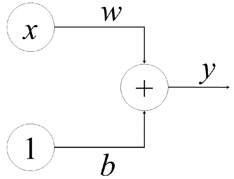
To understand how a neural network works, let us start with its basic component—a neuron. Figure 1 shows a neuron with one input. The variable x represents an input value. Each neuron will be assigned a weight of w. When a value goes from left to right across a connection, it is multiplied by the weight of the connection. In this case, the input x will be multiplied by the corresponding w, and when it reaches the next neuron, the value becomes . The weight will require modification for the neural network to learn.
The value b is a specific type of weight known as a bias. Notice that, for a bias, there are no input data connected; instead, a value of one is placed. The bias allows the neuron to change its output independently. Here y is the value that the neuron eventually outputs. To obtain the output, the neuron adds all of the values received through its connections. In this example, the relation between the input and the output can be indicated as . The neural networks also support multiple inputs. Consider each node to be its own linear regression model, with input data, weights, a bias (or threshold), and an output. The generic relationship is shown in (1).
Recall that weights are assigned once an input layer has been identified [13]. These weights aid in determining the significance of any given variable, with bigger ones contributing more substantially to the output when compared to other inputs. All inputs are then multiplied by their weights and added together. After that, the output is processed by an activation function, which decides the output. If that output reaches a certain threshold, the node is activated, sending data to the next layer of the network. As a result, the output of one node becomes the input of the next.
2.1.1. Activation Function
An activation function is required to be applied to each output of a layer. This is because neural networks can only learn from linear relationships. Hence, we need to use the activation function to bend the line into a curve. It can be represented as:
The most commonly used activation function is called Rectified Linear Unit (ReLU). ReLU function maps the negative input to zero but keeps the positive input as usual.
2.1.2. Loss Function
After building the basic structure of a neural network, the loss function is used in solving the underlying problem [13]. The loss function measures the distance between the targeted value and the predicted value. The targeted value is provided together with the training data but is not visible to the neural network during training. The predicted value is the output of the neural network. There are many different kinds of loss functions; each serves a different purpose. To illustrate the problem, let us assume that we are solving a regression problem, where the output should be a numerical value. We use one of the common loss functions for regression problems, which is the mean absolute error (MAE). It will calculate the absolute difference between the target value and the predicted value. The loss function is critical because it helps to adjust the weight values for achieving better accuracy.
2.1.3. Optimizer
The optimizer is a method or an algorithm used to modify the weights to minimize the loss. Almost all optimization algorithms are categorized as stochastic gradient descent. These algorithms are iterative, and train a network in stages [13]. The following are the basic steps during training:
- Take a sample of training data and make predictions using the network;
- Measure the losses between the target values and the predicted values. Modify the weights in such a way that could reduce the losses;
- Repeat the steps until the loss is minimized. By doing that, we will eventually have a network that fits perfectly with the training data.
2.1.4. Epochs
Epoch implies how many times the entire training dataset is passed to the model to train [13]. In other words, with one epoch set, every datapoint in the dataset has gone through the model once. Obviously, high epochs may well increase the training accuracy since the model has had more chances to train with the same dataset and vice versa. However, simply setting high epochs may cause the model to overfit the training data. It means that the model memorizes the data rather than learning it. Similarly, low epochs may result in under-fitting, whereby the model has not learned enough yet.
2.2. Types of Neural Networks
Neural networks, sometimes referred as Artificial Neural Networks (ANNs), can be classified into different types. Each of them adopts a distinctive structure to determine their own rules. There are several forms of ANN, each with its own set of capabilities. Neural networks with three or more layers are known as deep neural networks. Table 1 summarizes the different types of neural networks.
2.3. Machine Learning Based Cryptanalysis
The relationship between the fields of cryptanalysis and machine learning was first discussed in 1991 [1]. The author investigated how each field can benefit from the use of techniques from the other. Some of the early operational computers were committed to cryptanalytic activities. The fact that those early computers could learn to execute tasks that humans find difficult, such as playing checkers, indicates the first application of machine learning. Eventually, the fast improvement of algorithms and technology has led to increased research into machine learning in the domain of cryptanalysis.
Neural networks were first applied to cryptanalyze the Data Encryption Standard (DES) in 1995 [2]. Both linear and differential cryptanalysis were studied in that attempt. Aside from that, machine learning techniques were also applied to carry out side-channel attacks. The experiment utilized the Least Squares Support Vector Machine (LS-SVM) algorithm to study the security of software implemented with the Advanced Encryption Standard (AES) [5]. As a side channel, power consumption was investigated. The findings suggest that the selection of machine learning parameters greatly affects the performance of the classification. In 2012, a known-plaintext attack was designed in such a way that a neural network was trained to decrypt the ciphertext without knowing the encryption key [6]. The attack was successfully implemented against the Data Encryption Standard (DES) and Triple-DES.
Furthermore, Greydanus demonstrated that, with a 3000-unit Long Short-Term Memory (LSTM), an RNN can learn the decryption function of the Enigma machine [7]. The model can also be used to launch known-plaintext attacks on the Vigenère cipher and Autokey ciphers. Furthermore, a supervised machine learning assisted automated framework, which uses a random forest of decision trees, was implemented to identify exploitable fault instances [8]. The experiments were conducted against block ciphers PRESENT and LED, and the average accuracy of the model was around 85%. Recently, a neural network model was implemented to find the location of faults in GRAIN-128a (with and without authentication). The results showed that neural networks could be used instead of correlation with greater efficiency [9]. The accuracy for locating the correct fault in GRAIN-128a (without/with authentication) was 0.9988 and 0.9799, respectively. Additionally, a deep neural network-based differential distinguisher for round reduced PRESENT cipher was developed [10]. It was implemented together with an MLP network to identify the differential characteristics in the block cipher PRESENT. Experimental results showed that the model could distinguish up to five rounds of PRESENT.
As observed from the discussion in this section, an increase in the use of machine learning approaches for cryptanalysis is observed in recent years and there are areas that can be further investigated. Hence, this paper aims to conduct this investigation against selected cryptographic schemes.
2.4. Our Contribution
We use deep learning models for the analysis of cryptographic schemes under a few different settings. These include:
- Classification of the correct key from a set of keys;
- Recovering the secret key for a random keyspace. This has been applied against S-DES and Speck under MLP and LSTM models. MLP models have shown comparatively better performance against S-DES;
- Recovering the secret key for a restricted keyspace. MLP based method is adapted from the work of So [4] and applied to Simeck and Katan. LSTM and CNN were not considered as they have shown poor performance when applied to S-DES.
A summary of our work is provided in Table 2. A conclusion from the work is that the method presented in the work of So [4] can be extended to other ciphers; however, this method seems to be relying solely on the bit occurrence probability of the text-based key. The application of this method to different ciphers produces very similar results, which leads to the conclusion that the method does not consider any features other than the bit occurrence probability of the text-based key.
3. Description of Methods Adapted for Neural Cryptanalysis
This section introduces several methods for designing the neural cryptanalyses models used in this paper. We use three different methods against different ciphers.
3.1. Attack Modeling with a Random Key
With this approach, we investigate the capability of the neural network against modern ciphers under a known-plaintext scenario. We then examine the trained neural network by measuring the model’s accuracy to predict the key used for the encryption. With this method, we want to explore the potential of neural networks solely trained with the plaintext–ciphertext pairs. The cipher is considered a black box as the model does not consider anything about the specific structure of the algorithm.
The plaintext is generated as a random binary bit combination, such that , where denotes the plaintext length. The key is generated as a random binary bit combination, such that , where . For any i, the probability that the ith key bit is one is 0.5. Similarly, the probability of the ith bit being zero is also 0.5. We use two different methods under this model.
3.1.1. Method 1: Identify the Correct Key from a Set of Keys
Under this method, the randomly generated plaintext is encrypted with a key chosen among a fixed possible set of keys. These keys are selected arbitrarily. For example, let us assume we choose the number of keys in the set to be five, then all of the plaintexts can only be encrypted using one of these five keys. Both the plaintext and ciphertext are then inserted into the neural network together with a label identifying the key used for the corresponding encryption during the training phase. For this example, the label here will be between values zero and four. During the validation phase, the job of the neural network is to predict which key (the label) is used to encrypt by looking at the plaintext and ciphertext pairs. For further illustration, let us assume a cipher with the architecture shown in Table 3.
Table 3 illustrates a hypothetical cipher with a block size of four and a key size of four. For this example, the number of possible keys will be , but now we choose the number of keys in the set to be four: 0000, 0100, 0101 and 1011. These are the available keys that can be used throughout the experiment. That means the randomly generated 4-bit plaintext will be encrypted with only either one of these four keys. Each of the four keys will be given a label ranging from 0 to 3. During the training phase, we concatenate the 4-bit plaintext with the 4-bit ciphertext as the input for the neural network to learn. The expected output is the label of the key.
However, method 1 has its limitations when the key size becomes larger because a larger key size increases the complexity of the cipher. Therefore, S-DES with a key size of 10-bit is reasonable to investigate against this approach. S-DES has experimented with this method by setting the as 1024. On the other hand, the application of this method on Speck32/64 produced a result equivalent to a random guess, so we decided to reduce the round of Speck. This method was applied on round-reduced Speck with the as two, four, and ten. We started the experiments by testing a one round Speck. We then gradually increased the round count if it resulted in an accuracy better than the random guess.
3.1.2. Method 2: Identify All Key Bits
While the previous method (method 1) focuses on finding the exact key from a set of keys, we use a slightly different method that emphasizes on dentifying each key bit individually. With this method, the neural network will be trained with plaintext–ciphertext pairs. In the validation phase, it is required to predict the key used for the encryption. The way to measure the accuracy of this approach is by looking at the number of correct predictions among all the key bits.
For instance, we take the cipher assumption in Table 4 as an example. Consider the scenario where a randomly generated 4-bit plaintext is encrypted using a randomly generated 4-bit key. The plaintext bits and the ciphertext bits are then concatenated together and fed to the neural network. However, this time, the task of the network is to predict the 4-bit encryption key by outputting the value of the four key bits.
Referring to Table 4, let us consider that the plaintext is 0001 and the key is 1111. After encryption, the ciphertext is 0110. During the validation phase, the neural network receives the input as 00010110 and, after training, it should predict 1111 as the output to get 100% accuracy. Otherwise, if 1010 is predicted, then the prediction accuracy will be 50% since only two out of four bits are predicted correctly. This method has been investigated against S-DES.
3.2. Attack Modeling with Restricted Keyspace
The method described in this section is adapted from the work of So [4]. Instead of attacking the round reduced ciphers, they demonstrated a successful attack on the full-round lightweight block ciphers Simon and Speck, where the keyspace was restricted to a set of 64 ASCII characters. The model architecture is almost the same as method 2 but with a little revision on the use of the key. In this method, a restricted keyspace, also known as the text key, will be used rather than a random key. The key is generated as any combination of 64 ASCII characters.
Meanwhile, in text key generation, for a 16-bit key that consists of two characters, we will need to randomly select two ASCII characters, each representing an 8-bit to form the 16-bit key. The neural network will be fed plaintext and ciphertext pairs as input during the training phase. During the validation, the model accuracy will be calculated by evaluating the predicted key with the actual key. We test this method against two lightweight block ciphers: Simeck32/64 and Katan32.
There is a bias when using the text-based key. The bias is caused by the occurrence probability of each key bit in the 64 ASCII characters. For example, the first bit of the text key is always zero, and the second bit is one with a probability of 0.828. Hence, we need to eliminate the bias using Equation (3) during the experiment’s calculation to obtain the correct information about the performance of bit accuracy. The relevant formula for calculating the deviation, is given as:
where represents the bit accuracy probability (BAP), and represents the occurrence probability of the ith key bit. By applying Equation (3), if a positive deviation is obtained, then the neural network is said to break the cipher successfully and vice versa. Finally, the majority decision concept illustrated in So’s work is used to calculate the expected required plaintext to perform the attack.
The M known plaintexts required to find the encryption key can be calculated using the majority decision concept. Suppose we have the same key that is used to encrypt M plaintext-ciphertext pairs. If we are likely to discover the ith key bit with a probability of , then the likelihood of the attack success to discover the ith key bit, which is the likelihood of a valid majority decision, , is given as below [4]:
For large M this can be approximated to the Binomial distribution, :
The number of known plaintexts necessary to discover the ith key bit with a success probability greater than or equal to is:
4. Neural Cryptanalysis of Selected Ciphers
We conducted experiments on selected ciphers based on the methods described in Section 3. We first verified the implementation of the chosen ciphers with their test vectors. Next, we used the cipher implementation to generate plaintext–ciphertext pairs as training data for the next stage. The amount of training data was selected in the same way as with the original method [4]. For the building, training, and validation of the Deep Neural Network (DNN) model, at first, a baseline model, which holds the fundamental parameters setting of the neural network, was developed and tested with selected ciphers. The number of neurons in the input and output layers depends on the specific cipher. An exhaustive search through a manually specified subset of the hyperparameter space, and , is conducted to determine the number of hidden layers, H, and the number of neurons per hidden layer, N. After that, a decision was made to identify whether the experimental results can be improved. Different neural network models were tested, and their parameters were modified to improve the experimental results. Otherwise, another suitable cipher was examined by repeating the steps given.
The training loss and validation loss were observed to find out the suitable amount of epoch numbers for the experiments. The loss measures how well the model fits the respective data by calculating the difference between the predicted output with the actual output. We want the model to have a lower loss as much as possible since it represents that the model’s predictions are very close to the actual output. In general, it is best to stop training the model whenever the validation loss is minimum. As long as the validation loss keeps dropping, the epoch numbers should continue to be increased. However, if the validation loss starts to rise, then it might be a sign of overfitting. At this point, the training is terminated, and the best epoch number is selected. In short, the experiments with S-DES were done by manually starting with large enough epoch numbers and stopping the training whenever the optimum loss is found. However, it takes longer to train when a large dataset is used, especially for Simeck and Katan. Hence, an early stopping approach is used with these ciphers. The idea is similar, except that we utilize the callback function provided by Keras to stop the training automatically once the validation loss has stopped improving for at least a given epoch. The early stopping function will then revert the epoch numbers to the optimum.
We used Python programming language as a platform to perform all the tasks. Regarding the experimental environment setup, the Keras library with TensorFlow backend was used. All experiments were carried out on an Acer Aspire 5 equipped with a 2.7 GHz Intel Core i7 processor and 8 GB of RAM.
Different attack methods from Section 3 are applied to selected ciphers; namely, Simplified Data Encryption Standard (S-DES), Speck, Simeck and Katan. We discuss the implementation of the respective attacks and their results in the following sections. Note that the underlying cipher structure is considered a black box for all the experiments. Hence, we do not provide a detailed description of the ciphers in this paper.
4.1. Neural Cryptanalysis of S-DES
S-DES [14] is a simplified version of the Data Encryption Standard (DES) designed for education purposes. It consists of a block size of 8-bit and a key size of 10-bit. We apply two different attack models on S-DES. The proposed attacks on S-DES examine how the plaintext–ciphertext pairs can be used in training the neural network and searching the key. In the below sections, we first discuss existing machine learning-based analyses of S-DES, followed by our implementation models and the corresponding results.
4.1.1. Existing machine learning analysis of S-DES
Danziger and Amaral Henriques [15] applied MLP to attack the S-DES and analyzed it to find the relationship between differential and neural cryptanalysis. This work showed that the neural network was partially successful in recovering some of the key bits of S-DES. In a more recent work [4], the S-DES was claimed to be broken with a probability given known-plaintext bits.
4.1.2. Experiment 1: Choose from 1024 Key Sets
This experiment is conducted against S-DES using method 1 discussed in Section 3.1.1. The following describes the setups of the neural network as well as the input generation. Then, the remaining section discusses the results of the experiment. The hyperparameters of the model in this experiment are listed below:
- Input Layer: 16 neurons;
- Hidden Layers: details are presented in Table 5;
- Output Layer: 1024 neurons;
- Epochs: 50 rounds.
Note that the input layer of 16 neurons represents the combination of eight plaintext and eight ciphertext bits. The output layer of 1024 neurons indicate all the 1024 possible keys of S-DES. The number of epochs is set to 50 since 50 epochs are determined as optimal after testing several times.
A total of 200,000 datapoints (plaintext–ciphertext pairs with the label) are divided into training data and validation data with a ratio of 4:1. These data are generated by encrypting random plaintext with a random key. The generation of plaintext and ciphertext is pretty straightforward. We take eight random bits of plaintext and encrypt it with ten random key bits to form the 8-bit ciphertext. Since there are 1024 possible keys in S-DES, each is labeled as a number ranging from 0 to 1023. These values will be passed together with the plaintext–ciphertext pairs as labels for the model to train.
The model’s output is the predicted label (key used to encrypt the plaintext among 1024 possible sets). As long as the neural network outputs the label correctly, then it is counted as a success. This experiment is to validate the performance of a neural network to identify the correct key used during encryption from a set of keys of size 1024.
Table 5 shows the performance of different neural networks when method 1 is applied against S-DES.
Let us first look at the Multilayer Perceptrons (MLP) with only the hidden layers being manipulated. It shows how the number of hidden layers and the neuron numbers affect the accuracy of the model with the same input. Although based on a random guess, the accuracy should fall around 0.00098 (one divide by 1024), MLP 1 and MLP 4 failed to capture the training data pattern by having just 0.0011 accuracy. This is very close to the random guess. A possible explanation for this is that MLP 1, which has fewer parameters, faced difficulty in identifying the pattern while MLP 4, with five hidden layers, made it too complex for this situation. In terms of MLP 2, by doubling the neuron numbers in each layer, which increases the parameters to about 2.5 times, the model hit an accuracy of 0.2124. It was followed by further increasing the neuron number to a fairly large value for MLP 3, which also performed better than a random guess, but its accuracy did not take over the one that MLP 2 achieved. Lastly, experiments are also conducted using MLP 5 with two hidden layers of 1024 neurons. MLP 5 resulted in a similar accuracy as MLP 2. Although the number of hidden layers is reduced in MLP 5, the total parameters are four times larger than MLP 2.
By considering the training time, it may seem that MLP 2 is more suitable overall. Even though we ran the experiment on 50 epochs, we observe that some overfitting occurred since the validation accuracy does not match with the training accuracy. Note that most of the validation accuracy reported in Table 5 are floating around epoch 25, that is, the model does not improve anymore even though the training data is improving.
On the other hand, from the data in Table 5, it can be seen that the Convolutional Neural Network (CNN) performs poorly in this kind of problem with an accuracy of 0.0011. This is anticipated because CNN is designed to identify meaningful input data patterns that aid in detecting images or in the field of natural language processing but do not function well for cipher inputs as the data are purposely diffused.
4.1.3. Experiment 2: Predict the 10 Key Bits
This experiment is conducted against S-DES using method 2 discussed in Section 3.1.2. We first describe the setups of the neural network and the input generation. Then, we discuss the results of the experiment. The hyperparameters of the model in this experiment (method 2 against S-DES) are listed below:
- Input Layer: 16 neurons;
- Hidden Layers: details are presented in Table 6;
- Output Layer: 10 neurons;
- Epochs: 50 rounds.
Note that the input layer of 16 neurons represent the combination of eight plaintext bits and eight ciphertext bits. The output layer consists of ten neurons because the neural network just needs to predict the ten key bits of S-DES. The number of epochs is set to 50 since 50 epochs are determined as optimal after several testing.
A total of 200,000 datapoints (plaintext-ciphertext pairs with the label) are split into training data and validation data with a ratio of 4:1. These data are basically generated by encrypting random plaintext with a random key. We take eight random bits of plaintext, encrypt it with ten random bits of the key to form the 8-bit ciphertext. The ten key bits are then used as the label for the neural network to train. The output of the model is the ten predicted key bits.
Table 6 shows the performance of different neural networks when method 2 is applied against S-DES.
From Table 6, it can be seen that three different MLPs have been used, and they differ only in the number of hidden layers, which are five, four and three, respectively. It is apparent that the validation accuracies of the three neural networks are more or less the same. That means the accuracy does not affect the complexity of the neural network in this case. MLP 1 and MLP 2 both with roughly 1,000,000 parameters had a similar accuracy. Surprisingly, MLP 3, with about four times fewer parameters, still managed to achieve a similar accuracy or an even better accuracy than the more complex model. Supposedly, it is clear that the occurrence probability of the ten key bits should be 0.5 since they are generated randomly. As a result, these models that achieved a validation accuracy of about 0.72 are proven to perform better than the case of a random guess. In a nutshell, the results indicate that these models capture some information during the training phase; hence, have a better accuracy than the case of a random guess.
On top of that, a recurrent neural network using Long Short Term Memory (LSTM) was also included in the experiment. Unfortunately, by looking at the validation accuracy, we notice that LSTM does not help in solving the problem. A possible reason is that LSTM will have to make use of the recurrent property where the output will be fed back together with the input. In our case, the output prediction does not affect how the input behaves; thus, LSTM becomes ineffective for this problem.
4.2. Neural Cryptanalysis of Speck
The National Security Agency (NSA) officially published Speck in June 2013. Speck has been tuned for speed in software implementations. It was created for resource-constrained devices and gadgets that engage in the Internet of Things [16]. It supports several variants with a different number of blocks and key sizes. A block always consists of two words, although the words might be 16, 24, 32, 48, or 64 bits long. The matching key consists of two, three, or four words. The number of rounds is determined by the parameters used.
4.2.1. Existing Analysis of Speck
Dinur [11] developed an enumeration methodology for differential cryptanalysis, which may be used for all ten variants of Speck. Dinur claims that the framework is more efficient, particularly when the cipher employs a secret key that is greater than the block size. Another study reported that a differential attack can be applied on Speck with reduced rounds [17]. The authors achieved a differential attack on 10-round Speck32/64 with a time and data complexity of and , respectively. Furthermore, a recent research demonstrated that a ML-based differential distinguisher may be utilized to identify excellent input differences while attacking 11-round of Speck32/64 by lowering its security to 38 bits [3]. To the best of our knowledge, there is only one research that claimed to have successfully broken the full rounds of Speck32/64. So [4] claimed to attack the full round Speck with constrained key space. This is equivalent to method 3 of this paper.
4.2.2. Proposed Attack on Speck
In this section, we further investigate the application of method 1 by testing it against Speck. Since the full round Speck is quite strong, we started from a round-reduced Speck. The basic Speck32/64, which consists of a block size of 32-bit and key size of 64-bit, was used throughout the experiments. The number of key sets, , was chosen to be two, four and ten, respectively, for separate experiments to study the relationship betwen and corresponding accuracy. Note that method 3 is not applied to Speck in this paper since it has already been investigated in existing work [4]. The hyperparameters of the model in this experiment are listed below:
The input layer of 64 neurons represent the concatenated 32 plaintext and 32 ciphertext bits. The number of neurons in the output layer is dependent on the size of , that is, two, four or ten. The number of epochs is set to 20 as it was found optimal after several testing.
A total of 200,000 datapoints (plaintext–ciphertext pairs with the label) are split into training data and validation data with a ratio of 4:1. These data are generated by encrypting random plaintext with a random key. According to the key sets, , a number of keys are available for encryption. In this case, . Each was labeled with a value ranging from 0 to . We then take 32 random bits of plaintext, encrypt it with a 64-bit random key to form the 32-bit ciphertext. The plaintext–ciphertext pairs will be the input data for the model to train, while the label will be the expected output for the model to predict. The predicted label, that is, the key that is used to encrypt the plaintext, is the output of the model. In this case, the label will be the value ranging from 0 to , indicating the corresponding key used during encryption. As long as the neural network outputs the label correctly, then it was counted as a success.
Table 7 records the outcome of the experiments conducted against round-reduced Speck with a key set, . The tests were started with 1-round Speck. Next, we gradually incremented the number of rounds until the accuracy does not give better results than a random guess. We have selected some MLP based neural networks for these experiments because the previous findings in Section 4.1.2 and Section 4.1.3 have shown that multilayer perceptron (MLP) is better at solving classification problems than long short term memory (LSTM) and convolutional neural networks (CNN).
Based on Table 7, we noticed that the neural networks could break the 1-round Speck with very high accuracy. This can be clearly explained by looking at the key scheduler of Speck, where the first round key is not processed. Furthermore, all the neural networks had successfully broken the 2-round Speck when the is two. However, when it comes to the 3-round Speck, the best accuracy achieved among the three neural networks was 0.5024, which is not much better than the random guess of two items. It was the same case when we increased the value of ; the accuracy remained close to the probability of a random guess, that is, the neural networks fail to identify any information from the patterns. Hence, for Speck, the neural networks faced difficulties deriving useful clues with the plaintext–ciphertext pairs as input. They eventually failed to predict the correct encryption key beyond 2-round Speck.
4.3. Neural Cryptanalysis of Simeck
Simeck is a block cipher and first appeared in the proceeding of CHES 2015 [18]. It was strongly influenced by Simon and Speck; and integrated the good design components of these two ciphers to create a new block cipher family called Simeck. It utilizes a slightly modified version of Simon’s round function, where the rotation indices are changed from zero, five and one bit(s) to one, eight and two bit(s). The round function is reused in the key schedule as it is in Speck. Furthermore, Simeck makes use of the advantages of utilizing Linear Feedback Shift Register (LFSR)-based constants in the key scheduling to decrease the hardware footprints.
The variants of Simeck can be denoted as Simeck, where n represents the word size of 16, 24, or 32; while is the block size and is the key size. Simeck32/64, Simeck48/96, and Simeck64/128 are members of the Simeck family. Simeck32/64, for example, refers to the use of a 64-bit key to encrypt or decrypt the 32-bit message blocks.
Simeck is intended to have extremely small hardware footprints as well as compact software implementations. The structure is adopted by the round function and the key schedule algorithm. A plaintext is initially split into two words, and . The left word, , holds the most significant n bits and the right word, , holds the least significant n bits. Then, for a given number of rounds, Simeck round function is used to process these two words, and the two output words and are joined to produce a complete ciphertext, where T represents the total number of rounds. The interested reader may refer to the original description of Simeck for further details.
4.3.1. Existing Analysis of Simeck
In a recent work, Simeck was tested against linear cryptanalysis and it was claimed that the security of Simeck is inferior to that of its predecessors, Simon [19]. The author used Matsui’s algorithm to cover 14, 19 and 22 rounds of Simeck32/64, Simeck48/96 and Simeck64/128, respectively, while the best known linear attacks in corresponding Simon are 13, 16 and 19 rounds. Furthermore, a differential attack using dynamic key-guessing approach was demonstrated against Simeck [20]. The study claimed successful attacks on 22-round Simeck32, 28-round Simeck48 and 35-round Simeck64. Another research reports the first zero correlation linear cryptanalysis on 20/24/27 rounds of Simeck32/48/64, respectively [21]. Besides that, a work presented an improved integral cryptanalysis on reduced-round Simeck [22]. They demonstrate integral distinguishers against 22, 26 and 30 rounds Simeck32/64, Simeck48/96 and Simeck64/128, respectively. To the best of our knowledge, there are no publicly available machine-learning based analyses of Simeck.
4.3.2. Proposed Attack on Simeck
As discussed in Section 3.2, the text-based key approach (method 3) was shown to be effective in breaking the full rounds of Simon32/64 and Speck32/64. Hence, we further investigated the feasibility of method 3 on other similar ciphers. Consequently, Simeck was chosen because of its similarity of design structure to Simon and Speck. The hyperparameters of the model in this experiment are listed below:
- Input Layer: 64 neurons;
- Hidden Layers: described in Table 8;
- Output Layer: 64 neurons;
- Epochs: 100 rounds;
- Callback function: 5 patience, 0.0001 min delta.
The input layer of 64 neurons represents the concatenated 32 plaintext bits and 32 ciphertext bits. Because the neural network only needs to predict the 64 key bits in Simeck, the output layer is made up of 64 neurons. Additionally, after experimenting it with a few number of epochs, the symptoms of overfitting is observed. As a result, an early stop call back function is implemented to prevent from overfitting. That is, the training phase of the model is stopped and the best weights are reverted if the validation loss does not improve for at least the value of “min delta” for a duration of “patience” round. The “min delta” represents the minimum amount of change to count as an improvement.
A total of 500,000 data are generated for applying method 3 to Simeck. One-fifth of it is used as the validation data, while the rest of the data are used as the training data. In order to generate a 64-bit text-based key in Simeck, eight characters are required to be selected from the ASCII characters, where each character represents a specific 8-bit pattern. The generation of ciphertext is done by encrypting a random 32-bit plaintext with the 64-bit key. Lastly, the plaintext–ciphertext bit is fed into the neural network, and the 64-bit text key will be treated as the labels for the neural network to train. The output of the model is the 64 key bits that are predicted to be used for encrypting the plaintext.
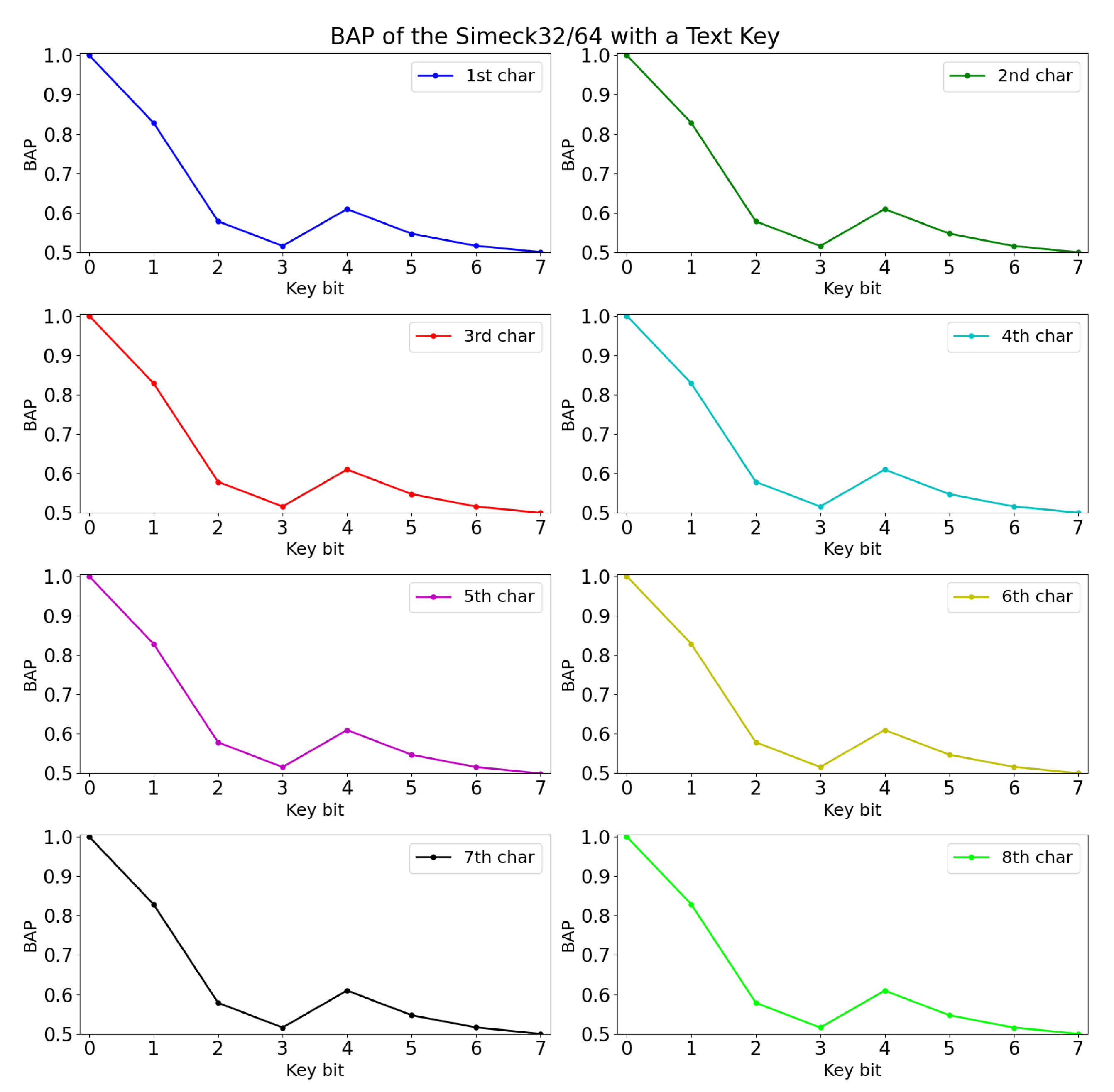
The experimental results are shown in Table 8. Among the three selected architectures, we found that MLP 1 performed slightly better in terms of validation accuracy. Hence, the experiments were conducted with MLP 1, and the findings were recorded for BAP calculation. The BAP of Simeck32/64 with the text key is shown in Figure 2 in the unit of character.
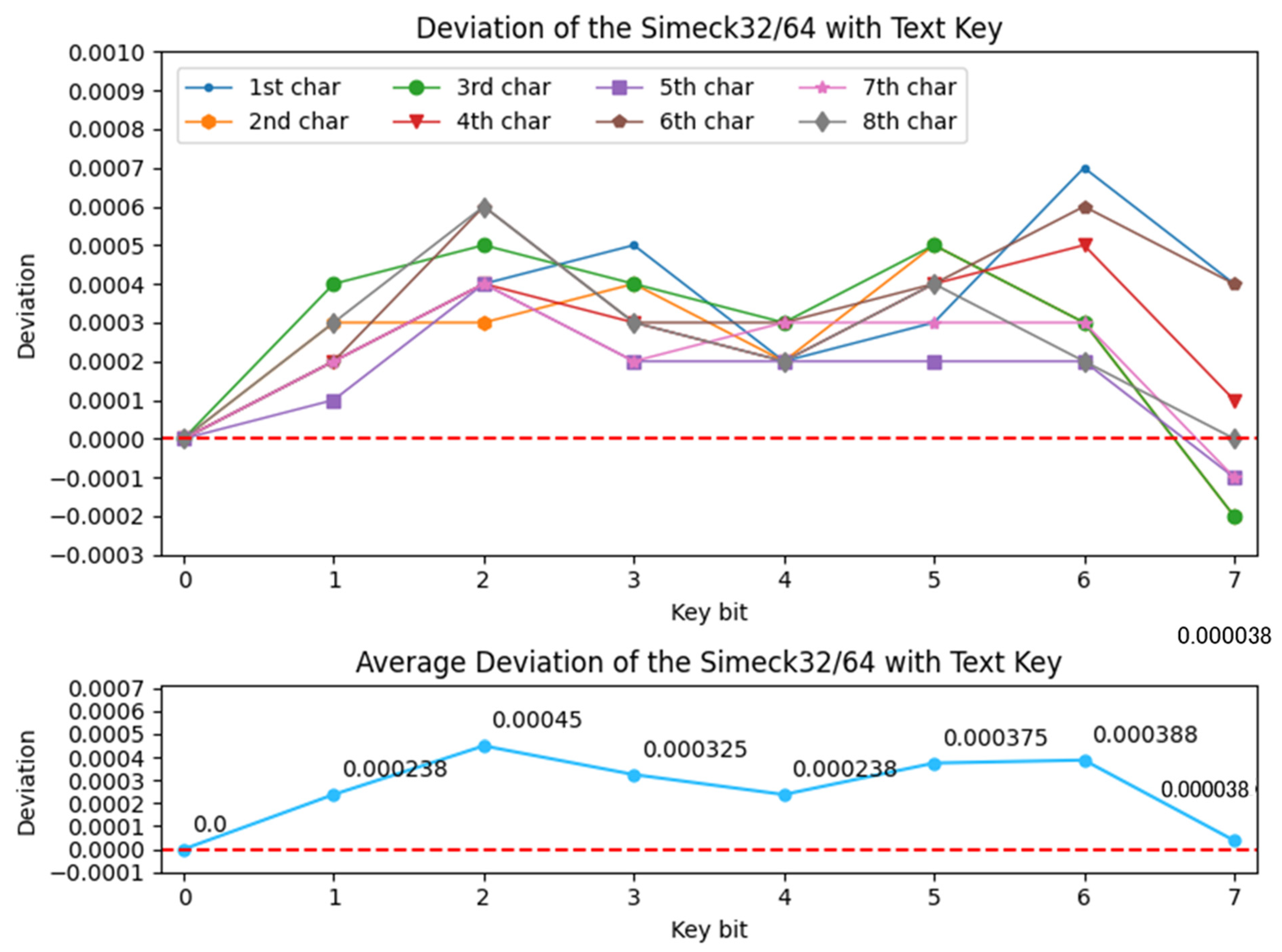
Based on the figure, it is noticed that the BAP for all the key bits of each character overlaps at nearly the same points. Furthermore, the slope of the graph is similar to the text key occurrence probability. This is because the neural network learns the training data features from the text-based key application. We notice that there is a small gap (deviation) between the BAP and occurrence probability of the text-based key. Therefore, the Equation (3) is used to calculate the deviation of BAP with the occurrence probability of the text-based key. The reason for calculating the deviation is to check whether the neural network model learns extra information when a text-based key is used. If a positive deviation is calculated then we expect that the model learns something new. The deviation of Simeck is calculated, and the results are shown in Figure 3.
Notice that the BAP is 1 for the 0th bit of the key. This is because the first bit of each byte is always zero in a text based key. In Figure 3, the neural network shows positive deviations when the bias of the text key is eliminated using Equation (3). For instance, using Binomial distribution, just known plaintext is required such that the key bit can be found with a probability of . Almost all key bits were laid above the positive deviation, indicating that the model could take advantage of the text key approach. Note that the last bit in each byte of the text-based key, that is, , laid below the negative deviation. Therefore, there is no significance in analyzing these because the given occurrence probability of the chosen text key is 0.5 at these respective bits. As a result, it was predicted that the neural network model did not gain extra information from the text-key based method for bit locations: .
4.4. Neural Cryptanalysis of Katan
Katan is a block cipher that was first proposed in CHES 2009 [23]. There are three variants of the cipher: Katan32, Katan48 and Katan64. The key schedule, which accepts an 80-bit key and 254 rounds, is shared by all ciphers in the Katan family, and so is the use of the same nonlinear functions. Katan ciphers have a relatively basic structure. The plaintext is input into two registers, , and . The plaintext length is determined by the block size. Each round, several bits are extracted from the registers and fed into two nonlinear Boolean functions. The two nonlinear Boolean function’s output is placed in the least significant bits of the registers. To ensure sufficient mixing of the inputs, the cipher is iterated for 254 rounds of updates.
4.4.1. Existing Analysis of Katan
Knellwolf used the linear key expansion strategy to adapt the meet-in-the-middle approach against Katan. In this way, for the full round Katan32, an attack with a complexity of was claimed [24]. Furthermore, automatic tools have been used to improve conditional differential cryptanalysis so that the meet-int-the-middle key recovery attack could be applied to Katan. By using the related-key scenario, the author has demonstrated successful key recovery attacks for 120, 103 and 90 of 254 rounds of Katan32, Katan48 and Katan64, respectively [25]. Besides that, recent research has presented the first linear cryptanalysis of Katan. This work analyzed the security of Katan against linear attack without neglecting the dependency of input S-box bits (the AND operation) [26]. This work claimed a single key known-plaintext attack against 131, 120 and 94 rounds of Katan32, Katan48 and Katan64, respectively. To the best of our knowledge, there are no publicly available machine learning-based security analyses of Katan.
4.4.2. Proposed Attack on Katan
Other than examining the approach with the text-based key (method 3) on Simeck, which has a similar design structure as the Simon and Speck, it would be better to validate the method on a lightweight block cipher that is not closely related to Simon and Speck. As a result, Katan was chosen for this purpose as it has a completely different architecture. The hyperparameters of the model in this experiment are listed below:
- Input Layer: 64 neurons;
- Hidden Layers: described in Table 9;
- Output Layer: 80 neurons;
- Epochs: 100 rounds;
- Callback function: 5 patience, 0.0001 min delta.
Note that the input layer of 64 neurons represent the concatenated 32 plaintext bits and 32 ciphertext bits. Because the neural network only needs to predict the 80 key bits in Katan32, the output layer comprises 80 neurons. A similar call back function as mentioned in Section 4.3.2 is used to prevent overfitting.
A total of 500,000 datasets are generated for applying method 3 against Katan. One-fifth of it is used as the validation data, while the rest is used as the training data. In order to generate an 80-bit text-based key, ten characters are required to be selected from the ASCII characters. The generation of ciphertext is done by encrypting a random 32-bit plaintext with the 80-bit key. Lastly, the plaintext–ciphertext pairs are fed into the neural network to train. The 80-bit text keys are treated as the labels. The output of the model is the 80 key bits that are predicted to be used for the encryption of the plaintext.
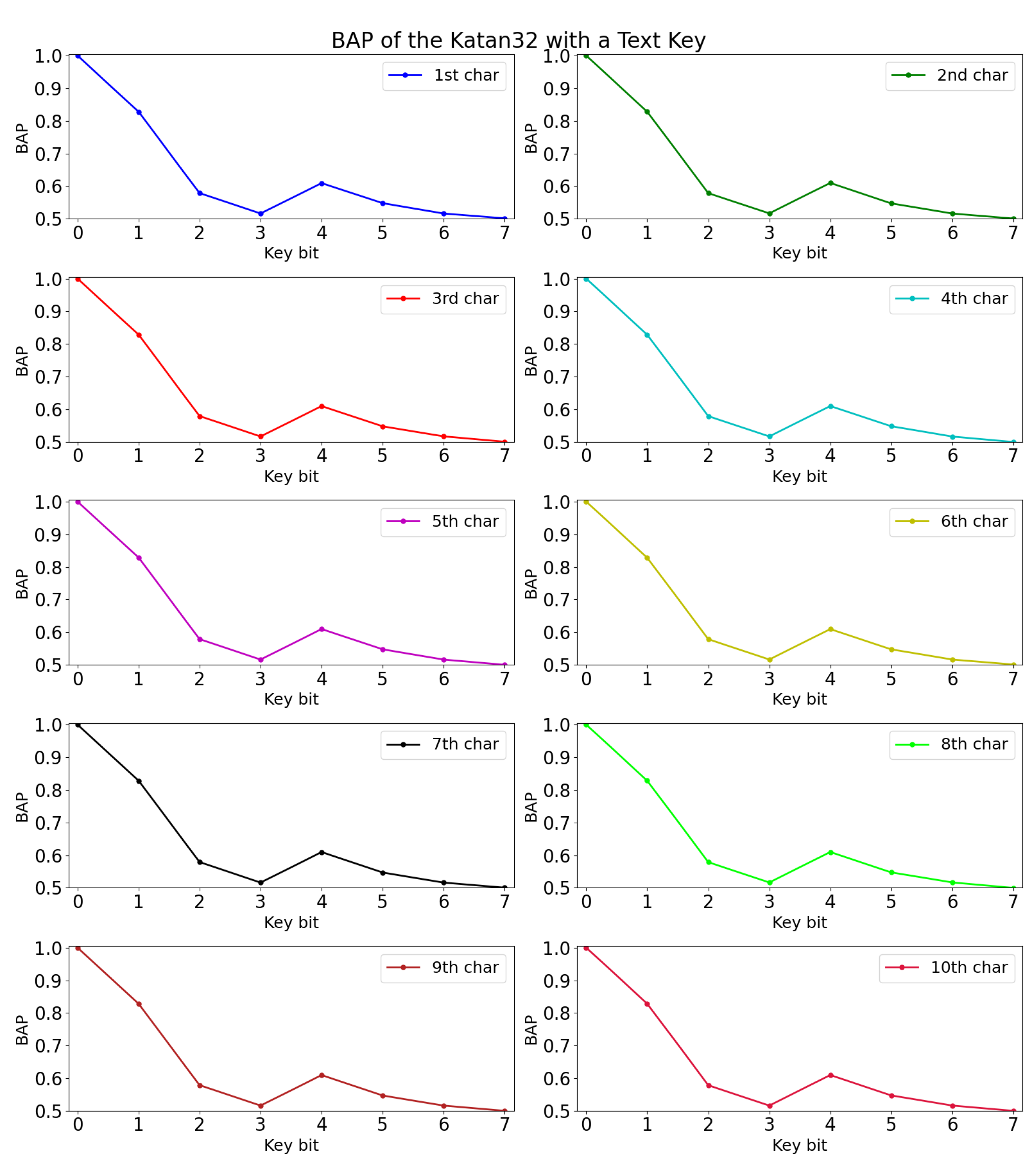
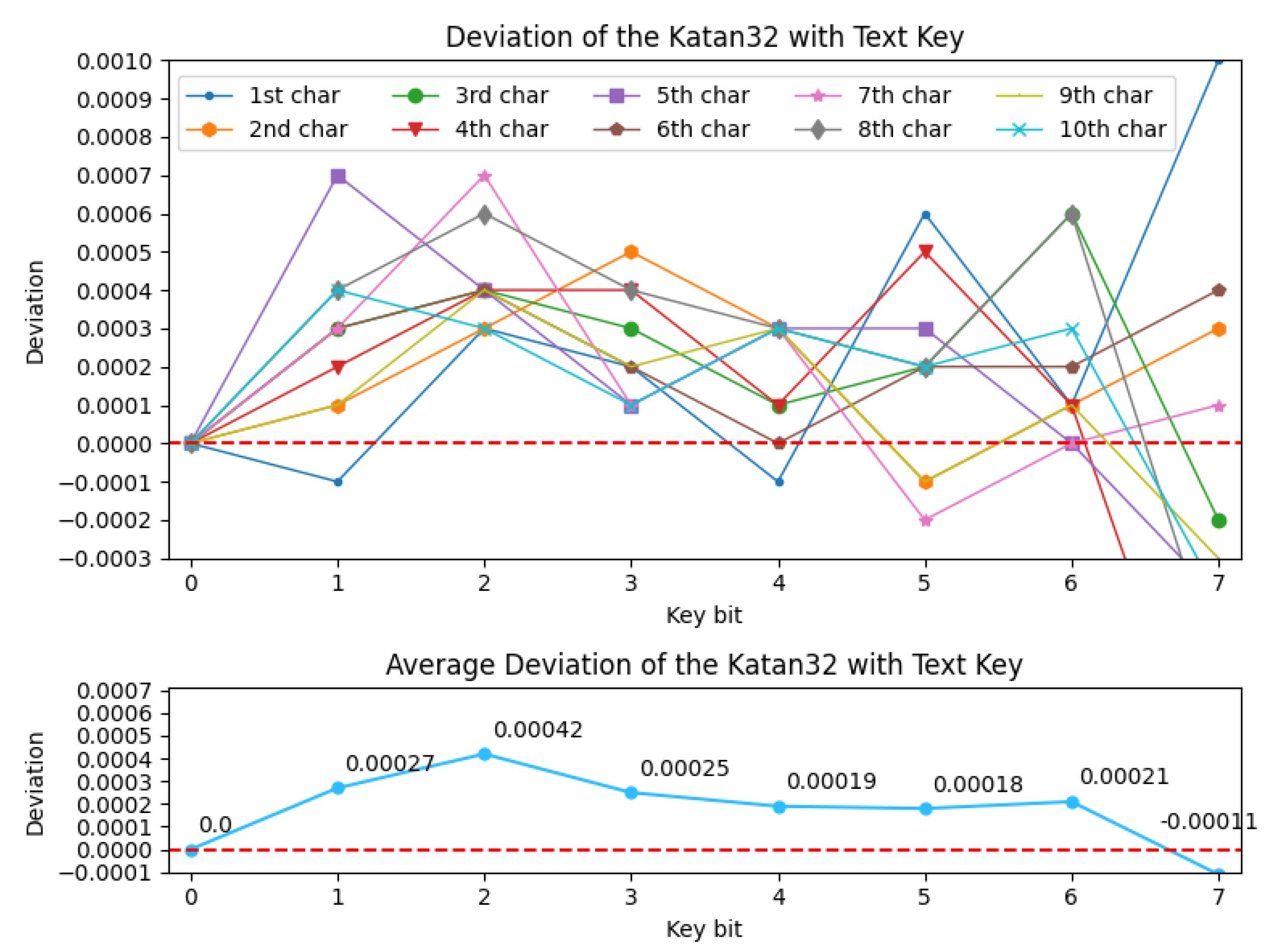
The experimental results are shown in Table 9. Among the three selected architectures, we found that MLP 1 performed slightly better in the validation accuracy. The BAP of Katan32 with the text key is shown in Figure 4 in units of character. We are able to obtain a positive deviation in Figure 5 after eliminating the bias (occurrence probability) of text key in Katan32 using Equation (3).
Since positive deviation is calculated and plotted in Figure 5, it can be inferred that the corresponding key bits of Katan32 can be recovered. Again, assuming Binomial distribution, we are able to find the key that are used for encryption by looking at the minimum BAP key bit. Similar to the case in Simeck, the last bit in each byte of the text-based key for Katan, i.e., , have a negative deviation. The negative deviation is because the occurrence probability of the chosen text key is 0.5 at these bits. Therefore, using method 3, the neural network does not gain any new information for these bits in Katan.
5. Conclusions
This paper investigated the applicability of deep learning models for the security analysis of cryptographic algorithms. A few neural network models have been implemented to conduct the experiments using method 1 against S-DES and round reduced Speck32/64. For S-DES, the full keyspace is used and tested with MLP and CNN models. Based on the results, CNN performed poorly for this task, while some of the MLP models showed better results than the random guess. The best model could achieve an accuracy of 0.2157. It is much better than a random guess, which has an accuracy of 0.0009. This implies that a neural network model can partially classify the correct key that is used for S-DES encryption. For Speck, method 1 performed well in 1-round Speck. However, experimental results indicate that it is challenging to apply method 1 beyond 2-round Speck when the key set is set to 2, 4 and 10. We also applied method 2 against S-DES using MLP and LSTM models. MLP models have shown relatively better performance and can recover the random key of S-DES with a probability better than the random guess. On the other hand, LSTM models failed to recover the random key of S-DES. However, both MLP and LSTM models in method 2 performed poorly against modern ciphers with larger block sizes.
We also adapted the text-key based approach and applied it to the block ciphers Simeck32/64 and Katan32. The results showed that the DL-based cryptanalysis model could find the text-based encryption key of the ciphers. Note that this method was previously applied to block ciphers Simon and Speck. This work confirms and validates that the text-based key approach is not only applicable to Simon and Speck but can also be applied to any other similar block ciphers. However, from the results of this paper and the earlier work [4], it seems that the neural network only learns the pattern of the bit occurrence probability of the ASCII characters. Notice that the training and validation accuracy results of Simeck and Katan are similar. We think that the similarity in the results is related to the bit occurrence probability of the text-based key. From the occurrence probability of the ASCII characters, we noticed that the bit accuracy probability (for both Simeck and Katan) closely follows the bit occurrence probability. We interpret that the neural networks learn the patterns of the bit occurrence probability and predict based on these patterns. For example, the first bit of the text key is always zero with a probability of one. Due to this, the neural network always predicts the first bit of each key byte to be zero. This is evident from the deviation when comparing the bit accuracy probability and the bit occurrence probability. Similarly, the last bit of the text key has an occurrence probability close to 0.5, resulting in a negative deviation while comparing the bit accuracy probability and bit occurrence probability. Therefore, for both Simeck and Katan, the neural network cannot obtain new information about the last bits in each byte of the text-based key. A limitation of method 3 is that the keyspace of this proposed DL-based cryptanalysis is confined to text-based keys.
Future research may be conducted to carefully investigate the possible representation of classical cryptanalysis weaknesses and convert them into inputs to train the neural network. The weaknesses could be based on existing attacks such as linear or differential cryptanalysis or any other form of known cryptanalyses. As long as the weaknesses are carefully represented and converted into inputs for the neural network to train, positive results may be derived. Another possible direction for future work may incorporate the cipher structure (instead of considering it a black box) with the different models from this paper.
Author Contributions
Conceptualization, B.Y.C.; methodology, B.Y.C.; validation, B.Y.C.; formal analysis, B.Y.C.; investigation, B.Y.C.; resources, I.S.; writing—original draft preparation, B.Y.C.; writing—review and editing, I.S.; supervision, I.S.; project administration, I.S.; funding acquisition, I.S. All authors have read and agreed to the published version of the manuscript.
Funding
This work is supported by the Ministry of Higher Education Malaysia through the Fundamental Research Grant Scheme (FRGS), project no. FRGS/1/2021/ICT07/XMU/02/1, as well as the Xiamen University Malaysia Research Fund under Grant XMUMRF/2019-C3/IECE/0005.
Institutional Review Board Statement
Not applicable.
Informed Consent Statement
Not applicable.
Data Availability Statement
All of the reported results are included in the manuscript. The datasets used for the experiments in this study are available on request from the corresponding author.
Conflicts of Interest
The authors declare no conflict of interest.
References
- Rivest, R.L. Cryptography and machine learning. In Advances in Cryptology—ASIACRYPT 1991; Lecture Notes in Computer Science; Imai, H., Rivest, R.L., Matsumoto, T., Eds.; Springer: Berlin/Heidelberg, Germany, 1991; Volume 739, pp. 427–439. [Google Scholar] [CrossRef]
- Dourlens, S.; Neuro-Cryptography, M.S. Department of Microcomputers and Microelectronics. Master’s Thesis, University of Paris, Paris, France, 1995. [Google Scholar]
- Gohr, A. Improving Attacks on Round-Reduced Speck32/64 Using Deep Learning. In Advances in Cryptology—CRYPTO 2019; Lecture Notes in Computer Science; Boldyreva, A., Micciancio, D., Eds.; Springer: Cham, Germany, 2019; Volume 11693, pp. 150–179. [Google Scholar] [CrossRef]
- So, J. Deep learning-based cryptanalysis of lightweight block ciphers. Secur. Commun. Netw. 2020, 2020, 3701067. [Google Scholar] [CrossRef]
- Hospodar, G.; Gierlichs, B.; De Mulder, E.; Verbauwhede, I.; Vandewalle, J. Machine learning in side-channel analysis: A first study. J. Cryptogr. Eng. 2011, 1, 293. [Google Scholar] [CrossRef]
- Alani, M.M. Neuro-cryptanalysis of DES and Triple-DES. In Neural Information Processing—ICONIP 2012; Lecture Notes in Computer Science; Huang, T., Zeng, Z., Li, C., Leung, C.S., Eds.; Springer: Berlin/Heidelberg, Germany, 2012; Volume 7667, pp. 637–646. [Google Scholar] [CrossRef]
- Greydanus, S. Learning the Enigma with recurrent neural networks. arXiv 2012, arXiv:1708.07576. [Google Scholar]
- Saha, S.; Jap, D.; Patranabis, S.; Mukhopadhyay, D.; Bhasin, S.; Dasgupta, P. Automatic characterization of exploitable faults: A machine learning approach. IEEE Trans. Inf. Forensics Secur. 2019, 14, 954–968. [Google Scholar] [CrossRef]
- Baksi, A.; Sarkar, S.; Siddhanti, A.; An, R.; Chattopadhyay, A. Differential fault location identification by machine learning. CAAI Trans. Intell. Technol. 2021, 6, 17–24. [Google Scholar] [CrossRef]
- Jain, A.; Kohli, V.; Mishra, G. Deep learning based differential distinguisher for lightweight cipher PRESENT. IACR Cryptol. ePrint Arch. 2020, 2020, 846. [Google Scholar]
- Dinur, I. Improved differential cryptanalysis of round-reduced Speck. In Selected Areas in Cryptography—SAC 2014; Lecture Notes in Computer Science; Joux, A., Youssef, A., Eds.; Springer: Cham, Switzerland, 2014; Volume 8781, pp. 147–164. [Google Scholar] [CrossRef] [Green Version]
- Baksi, A.; Breier, J.; Chen, Y.; Dong, X. Machine learning assisted differential distinguishers for lightweight ciphers. In Proceedings of the 2021 Design, Automation & Test in Europe Conference & Exhibition—DATE 2021, Grenoble, France, 1–5 February 2021; pp. 176–181. [Google Scholar] [CrossRef]
- Goodfellow, I.; Bengio, Y.; Courville, A. Deep Learning; MIT Press: Cambridge, MA, USA, 2016. [Google Scholar]
- Schaefer, E.F. A simplified data encryption standard algorithm. Cryptologia 1996, 20, 77–84. [Google Scholar] [CrossRef]
- Danziger, M.; Henriques, M.A.A. Improved cryptanalysis combining differential and artificial neural network schemes. In Proceedings of the International Telecommunications Symposium—ITS 2014, Sao Paulo, Brazil, 17–20 August 2014; pp. 1–5. [Google Scholar] [CrossRef]
- Beaulieu, R.; Shors, D.; Smith, J.; Treatman-Clark, S.; Weeks, B.; Wingers, L. The SIMON and SPECK lightweight block ciphers. In Proceedings of the 52nd ACM/EDAC/IEEE Design Automation Conference—DAC 2015, San Francisco, CA, USA, 7–11 June 2015; pp. 1–6. [Google Scholar] [CrossRef]
- Abed, F.; List, E.; Lucks, S.; Wenzel, J. Differential cryptanalysis of round-reduced Simon and Speck. In Fast Software Encryption—FSE 2014; Lecture Notes in Computer Science; Cid, C., Rechberger, C., Eds.; Springer: Berlin/Heidelberg, Germany, 2015; Volume 8540, pp. 525–545. [Google Scholar] [CrossRef]
- Yang, G.; Zhu, B.; Suder, V.; Aagaard, M.D.; Gong, G. The Simeck family of lightweight block ciphers. In Cryptographic Hardware and Embedded Systems—CHES 2015; Lecture Notes in Computer Science; Güneysu, T., Handschuh, H., Eds.; Springer: Berlin/Heidelberg, Germany, 2015; Volume 9293, pp. 307–329. [Google Scholar] [CrossRef] [Green Version]
- Bagheri, N. Linear cryptanalysis of reduced-round SIMECK variants. In Progress in Cryptology—INDOCRYPT 2015; Lecture Notes in Computer Science; Biryukov, A., Goyal, V., Eds.; Springer: Cham, Germany, 2015; Volume 9462, pp. 140–152. [Google Scholar] [CrossRef]
- Qiao, K.; Hu, L.; Sun, S. Differential security evaluation of Simeck with dynamic key-guessing techniques. In Proceedings of the 2nd International Conference on Information Systems Security and Privacy—ICISSP 2016, Rome, Italy, 19–21 February 2016; pp. 74–84. [Google Scholar] [CrossRef] [Green Version]
- Zhang, K.; Guan, J.; Hu, B.; Lin, D. Security evaluation on Simeck against zero-correlation linear cryptanalysis. IET Inf. Secur. 2018, 12, 87–93. [Google Scholar] [CrossRef] [Green Version]
- Li, H.; Ren, J.; Chen, S. Improved integral attack on reduced-round Simeck. IEEE Access 2019, 7, 118806–118814. [Google Scholar] [CrossRef]
- De Cannière, C.; Dunkelman, O.; Knežević, M. KATAN and KTANTAN—A family of small and efficient hardware-oriented block ciphers. In Cryptographic Hardware and Embedded Systems—CHES 2009; Lecture Notes in Computer Science; Clavier, C., Gaj, K., Eds.; Springer: Berlin/Heidelberg, Germany, 2009; Volume 5747, pp. 272–288. [Google Scholar] [CrossRef]
- Knellwolf, S. Accelerated key search for the KATAN family of block ciphers. In Proceedings of the ECRYPT Workshop on Lightweight Cryptography, Louvain-la-Neuve, Belgium, 28–29 November 2011. [Google Scholar]
- Knellwolf, S.; Meier, W.; Naya-Plasencia, M. Conditional differential cryptanalysis of Trivium and KATAN. In Selected Areas in Cryptography—SAC 2011; Lecture Notes in Computer Science; Miri, A., Vaudenay, S., Eds.; Springer: Berlin/Heidelberg, Germany, 2012; Volume 7118, pp. 200–212. [Google Scholar] [CrossRef]
- Shi, D.; Hu, L.; Sun, S.; Song, L. Linear(hull) cryptanalysis of round-reduced versions of KATAN. In Proceedings of the 2nd International Conference on Information Systems Security and Privacy—ICISSP 2016, Rome, Italy, 19–21 February 2016; pp. 364–371. [Google Scholar] [CrossRef]
Figure 1.
A linear unit with one input.

Figure 2.
BAP of Simeck with text key.

Figure 3.
Deviation of Simeck with text key.

Figure 4.
BAP of Katan with text key.

Figure 5.
Deviation of Katan with text key.


Table 1.
Types of neural networks [13].
Table 1.
Types of neural networks [13].
| Model | Description |
|---|---|
| Feed Forward Neural Network |
|
| Multilayer Perceptron (MLP) |
|
| Convolutional Neural Network (CNN) |
|
| Recurrent Neural Network (RNN) |
|
| Long Short-Term Memory (LSTM) |
|
Table 2.
Summary of our results and comparison with existing works.
| Cipher | Outcome |
|---|---|
| S-DES |
|
| Speck |
|
| Simeck and Katan |
|
Table 3.
A hypothetical cipher architecture for illustration purposes.
| Block size | 4 |
| Key size | 4 |
| Number of keys, | |
| All possible keys, K | K = 0000, 0001, 0010, 0011, 0100, 0101, 0110, 0111, 1000, 1001, 1010, 1011, 1100, 1101, 1110, 1111 |
| Key sets, | 4 |
| Selected keys, k | |
| Labeling | “0000”: 0, “0100”: 1, “0101”: 2, “1011”: 3 |
Table 4.
Generation of input and prediction of output.
| Plaintext | 0001 |
| Key | 1111 |
| Ciphertext | 0110 |
| Neural network receives | 00010110 |
| Correct prediction | 1111 |
| Prediction 1: 1111 | 100% accuracy |
| Prediction 2: 1010 | 50% accuracy |
Table 5.
Results of experiment 1 on S-DES (16 input layers and 1024 output layers).
| Network | Hidden Layers | Total Parameters | Train Time (s) | Train Accuracy | Validation Accuracy |
|---|---|---|---|---|---|
| MLP 1 | 128, 256, 128 | 200,192 | 730.62 | 0.0013 | 0.0011 |
| MLP 2 | 256, 512, 256 | 530,432 | 1420.81 | 0.3968 | 0.2124 |
| MLP 3 | 1024, 1024, 1024 | 3,166,208 | 6877.16 | 0.3785 | 0.1540 |
| MLP 4 | 512, 512, 512, 512, 512 | 1,584,640 | 4205.37 | 0.0013 | 0.0011 |
| MLP 5 | 1024, 1024 | 2,116,608 | 5151.20 | 0.4680 | 0.2157 |
| CNN 1 | 128, 64 | 104,272 | 692.95 | 0.0013 | 0.0011 |
| CNN 2 | 512, 256, 256 | 576,144 | 1587.95 | 0.0013 | 0.0011 |
Table 6.
Results of experiment 2 on S-DES (16 input layers and 10 output layers).
| Network | Hidden Layers | Total Parameters | Train Time (s) | Train Accuracy | Validation Accuracy |
|---|---|---|---|---|---|
| MLP 1 | 512, 512, 512, 512, 512 | 1,064,458 | 1615.96 | 0.8072 | 0.7269 |
| MLP 2 | 256, 512, 1024, 512 | 1,191,178 | 1705.5 | 0.817 | 0.7261 |
| MLP 3 | 256, 512, 256 | 269,834 | 375.17 | 0.7952 | 0.7291 |
| LSTM 1 | 32, 50, 50 | 41,622 | 3248.35 | 0.5000 | 0.4998 |
| LSTM 2 | 50, 100, 50 | 101,510 | 4970.78 | 0.5003 | 0.4989 |
| LSTM 3 | 100, 200, 64 | 350,090 | 9016.15 | 0.5005 | 0.5002 |
Table 7.
Results of method 1 on Speck (64 input layers and output layers).
| Network | Hidden Layers | Round | Accuracy | ||
|---|---|---|---|---|---|
| MLP 1 | 128, 256, 128 | 1 | 1.0000 | 1.0000 | 0.8985 |
| 2 | 0.9728 | 0.2507 | 0.1001 | ||
| 3 | 0.5009 | - | - | ||
| MLP 2 | 256, 512, 256 | 1 | 1.0000 | 1.0000 | 0.8967 |
| 2 | 0.9831 | 0.2559 | 0.1006 | ||
| 3 | 0.5017 | - | - | ||
| MLP 3 | 1024, 1024, 1024 | 1 | 1.0000 | 1.0000 | 0.9539 |
| 2 | 0.9949 | 0.2498 | 0.1175 | ||
| 2 | 0.5024 | - | - | ||
Table 8.
Results of method 3 against Simeck (64 input and output layers).
| Network | Hidden Layers | Total Param. | Train Time (s) | Train Accur. | Validation Accuracy |
|---|---|---|---|---|---|
| MLP 1 | 512, 512, 512, 512, 512 | 1,116,736 | 897.96 | 0.6368 | 0.6369 |
| MLP 2 | 1024, 1024, 1024, 1024, 1024 | 4,330,560 | 2802.39 | 0.6367 | 0.6367 |
| MLP 3 | 256, 256, 256, 256, 256 | 296,256 | 171.48 | 0.6367 | 0.6368 |
Table 9.
Results of method 3 against Katan (64 input layers and 80 output layers).
| Network | Hidden Layers | Total Param. | Train Time (s) | Train Accur. | Validation Accuracy |
|---|---|---|---|---|---|
| MLP 1 | 512, 512, 512, 512, 512 | 1,124,944 | 902.18 | 0.6369 | 0.6370 |
| MLP 2 | 1024, 1024, 1024, 1024, 1024 | 4,346,960 | 3102.95 | 0.6368 | 0.6367 |
| MLP 3 | 256, 256, 256, 256, 256 | 300,368 | 179.84 | 0.6367 | 0.6368 |
Publisher’s Note: MDPI stays neutral with regard to jurisdictional claims in published maps and institutional affiliations. |
© 2021 by the authors. Licensee MDPI, Basel, Switzerland. This article is an open access article distributed under the terms and conditions of the Creative Commons Attribution (CC BY) license (https://creativecommons.org/licenses/by/4.0/).
Share and Cite
MDPI and ACS Style
Chong, B.Y.; Salam, I. Investigating Deep Learning Approaches on the Security Analysis of Cryptographic Algorithms. Cryptography 2021, 5, 30. https://doi.org/10.3390/cryptography5040030
AMA Style
Chong BY, Salam I. Investigating Deep Learning Approaches on the Security Analysis of Cryptographic Algorithms. Cryptography. 2021; 5(4):30. https://doi.org/10.3390/cryptography5040030
Chicago/Turabian StyleChong, Bang Yuan, and Iftekhar Salam. 2021. "Investigating Deep Learning Approaches on the Security Analysis of Cryptographic Algorithms" Cryptography 5, no. 4: 30. https://doi.org/10.3390/cryptography5040030