
Ab Initio Phase Diagram of Copper


1
Los Alamos National Laboratory, Los Alamos, NM 87545, USA
2
MALTA Consolider Team, Departamento de Física Aplicada-ICMUV, Universidad de Valencia, Edificio de Investigación, C/Dr. Moliner 50, 46100 Valencia, Spain
*
Author to whom correspondence should be addressed.
†
These authors contributed equally to this work.
Crystals 2021, 11(5), 537; https://doi.org/10.3390/cryst11050537
Submission received: 13 April 2021
/
Revised: 4 May 2021
/
Accepted: 5 May 2021
/
Published: 12 May 2021
(This article belongs to the Special Issue Properties of Transition Metals and Their Compounds at Extreme Conditions)
Abstract
:Copper has been considered as a common pressure calibrant and equation of state (EOS) and shock wave (SW) standard, because of the abundance of its highly accurate EOS and SW data, and the assumption that Cu is a simple one-phase material that does not exhibit high pressure (P) or high temperature (T) polymorphism. However, in 2014, Bolesta and Fomin detected another solid phase in molecular dynamics simulations of the shock compression of Cu, and in 2017 published the phase diagram of Cu having two solid phases, the ambient face-centered cubic (fcc) and the high- body-centered cubic (bcc) ones. Very recently, bcc-Cu has been detected in SW experiments, and a more sophisticated phase diagram of Cu with the two solid phases was published by Smirnov. In this work, using a suite of ab initio quantum molecular dynamics (QMD) simulations based on the Z methodology, which combines both direct Z method for the simulation of melting curves and inverse Z method for the calculation of solid–solid phase boundaries, we refine the phase diagram of Smirnov. We calculate the melting curves of both fcc-Cu and bcc-Cu and obtain an equation for the fcc-bcc solid–solid phase transition boundary. We also obtain the thermal EOS of Cu, which is in agreement with experimental data and QMD simulations. We argue that, despite being a polymorphic rather than a simple one-phase material, copper remains a reliable pressure calibrant and EOS and SW standard.
1. Introduction
Copper is one of the most studied d-block transition metals. It is a common pressure calibrant because of the availability of its accurate shock compression data [1,2,3]. Copper has also been used to calibrate two of the important standards for static X-ray diffraction experiments, ruby and gold [4]. Copper is useful because it provides more accurate pressure (P) determination than other standards, including Pt, Mo, and W, due to its larger compressibility and the presumed lack of phase changes. Indeed, previous shock studies suggest that Cu remains in face-centered cubic (fcc) structure from ambient conditions until melting [5]. These studies reached peak conditions by utilizing a single shock. Using ramp compression, in which peak conditions are reached through a series of shocks, the ambient fcc phase is observed to be stable to TPa pressures [6]. However, a metastable body-centered cubic (bcc) structure is observed in the pseudomorphic Cu films grown on the surfaces of Pd, Pt, Ag, and Fe, or as small precipitates in a bcc-Fe matrix [7], and is suggested to possibly be stable at higher temperatures [8]. A recent computational study by Neogi and Mitra [9] based on density functional theory (DFT) suggests the possible existence of a bcc or body-centered tetragonal (bct) structure at a temperature (T) of 1520 K and GPa. In 2019, Sims et al. [10] completed a series of laser shock experiments with in situ X-ray diffraction using the Dynamic Compression Sector at Argonne National Laboratory in order to study the phase diagram and melting curve of Cu. At GPa they observed the appearance of bcc-Cu with a density of 14.02 g/cc. The bcc phase consistently coexists with melt, suggesting a high thermodynamic, or possibly kinetic barrier to transformation. The experimental Ts were higher than those in the ramp compression studies, which implies that bcc-Cu is thermodynamically stable at high T only. In a more recent X-ray diffraction study of shock-compressed copper by Sharma et al. [11] the fcc-bcc transformation is observed at ∼180 GPa; specifically, the line profile of Cu at 181.5 GPa shows the appearance of a new peak indexed as the bcc peak that partially overlaps with the fcc peak indicating a mixed fcc-bcc phase. At 211.5 GPa the fcc peaks completely disappear and two additional and bcc peaks appear instead, which implies a wide P interval of ∼30 GPa of fcc-bcc coexistence in the shock-wave experiment.
The physical properties of bcc-Cu have been studied theoretically using both classical and ab initio approaches. At ambient P and , bcc-Cu is mechanically unstable it becomes mechanically stable at GPa at [12], or above ∼600 K at [13]. The equations of state of both fcc-Cu and bcc-Cu are predicted to be very close to each other [12], in terms of the very similar values of the corresponding atomic volumes, bulk moduli, and their pressure derivatives. At ambient P, bcc-Cu is higher in energy than fcc-Cu by ∼2.9 mRy/atom, or ∼40 meV/atom [14], and their energy difference increases with increasing P [14] and/or volumetric strain [13]. As shown in [14], fcc-Cu remains the most thermodynamically stable solid structure of copper up to at least 10 TPa, which is confirmed by the very recent ramp compression experiments to 2.3 TPa [6]. However, as the example of niobium clearly demonstrates [15], an energy excess as high as ∼450 meV/atom can be overcome with the proper entropy gain by another solid structure at high T (in the case of Nb, it is the high-T orthorhombic Pnma vs. the ambient bcc), so that bcc-Cu can in principle be expected to become thermodynamically competitive with fcc-Cu at high In fact, as recent shock compression experiments demonstrate, bcc-Cu may be the physical solid phase of Cu at high-.
To the best of our knowledge, bcc-Cu was consistently studied for the first time by Bolesta and Fomin using classical molecular dynamics (CMD) code LAMMPS [16]. They simulated the shock-wave loading of fcc-Cu and observed a transition to bcc at P above ∼80 GPa and the corresponding T above ∼2000 K. Then, they calculated the phase diagram of Cu by considering both structures, and found out that bcc-Cu becomes thermodynamically stable at high- conditions; specifically, the fcc-bcc-liquid triple point is at = (80 GPa, 3490 K), and the entropy difference between the two solid structures at the triple point is [16]. Furthermore, Bolesta and Fomin were the first to detect the appearance of bcc-Cu above 100 GPa and 2000 K in molecular dynamic simulations of the shock compression of copper [17].
In a very recent paper, Smirnov [18] presents the phase diagrams of copper, silver and platinum calculated using a first principles based approach. He claims that all three substances are complex materials with at least two different solid phases on their phase diagrams. Specifically, all three phase diagrams contain both fcc (which is the ambient phase of each of the three substances) and bcc phases. The purpose of this work is to calculate the phase diagram of copper and to confirm that bcc does become the physical phase of copper at high- conditions.
To clarify the issues related to the phase diagram of copper, in the present work we carried out a systematic DFT-based study. Specifically, we calculated equations of state of both fcc and bcc, their melting curves using ab initio quantum molecular dynamics (QMD) simulations implemented with VASP (Vienna Ab initio Simulation Package), and estimated the P-T location of the fcc-bcc solid–solid phase transition boundary. Our theoretical results appear to be in excellent agreement with all the available relevant experimental data as well as the theoretical calculations of Bolesta and Fomin [16] and Smirnov [18].
2. Equations of State
For our theoretical study of the phase diagram of Cu, we used the following electron core-valence representation: [Mg] , i.e., we assigned the 17 outermost electrons of Cu to the valence. The valence electrons were represented with a plane-wave basis set with a cutoff energy of 460 eV, while the core electrons were represented by projector augmented-wave (PAW) pseudopotentials. We used the generalized gradient approximation (GGA) with the Perdew–Burke–Ernzerhof (PBE) exchange-correlation functional.
We first calculated the equations of state (EOS) of both fcc-Cu and bcc-Cu. We used unit cells with volumes that correspond to a P range of ∼−10–1000 GPa, and very dense k-point meshes of for fcc-Cu and for bcc-Cu. With such a dense k-point mesh, full energy convergence to 0.1 meV/atom is achieved in the whole P range for both fcc-Cu and bcc-Cu. The third-order Birch–Murnaghan forms of the two EOSs are (in the following stands for density, in g cmB and for bulk modulus, in GPa, and its pressure derivative, and the subscript 0 means
where and
In each of the two cases, this analytic form is expected to be reliable to ∼1000 GPa. So, indeed, the two EOSs are very similar to each other. Our value of coincides with the experimental one [19], and those of and for fcc-Cu are in excellent agreement with and from experiment [20].
We also note that the finite-T counterparts of the above two EOSs can be written approximately as
These values were chosen to match the two ambient melting points in the -T coordinates which are, respectively, from experiment [19,21], and from extrapolating our QMD data on the melting curve of bcc-Cu discussed below to
The reliability of these two “thermal EOSs” is demonstrated by comparing the values of the melting P () that they give when the corresponding s and melting Ts () are used to those that come directly from QMD melting simulations, see Table 1 and Table 2. Let us now show another example. The “thermal EOS” (1), (2) for bcc-Cu on the Hugoniot with P = 240 GPa and the corresponding T of 6721.1 K, which comes from along the Hugoniot discussed below, gives g cm in exact agreement with [10].
The similarity of the two sets of the EOS parameters and the corresponding two values of implies that, if the fcc-bcc phase transition does occur in Cu, at the transition the two volumes are expected to be close to each other, so that the corresponding volume change is small, and therefore the fcc-bcc phase transition boundary is rather flat, in view of the Clausius–Clapeyron formula. Our ab initio phase diagram of copper discussed below demonstrates exactly that.
3. Melting Curves
Our QMD melting simulations were carried out using the Z method implemented with VASP, which is described in detail in Refs. [22,23,24]. We used supercells of ∼500 atoms; specifically, a 500-atom ( one for fcc-Cu and a 512-atom one ( 109.5-rhombohedral) for bcc-Cu. The simulations were carried out with a single -point (with such a large supercell, full energy convergence, to 1 meV/atom, was achieved in every case considered) having 17 outermost electrons of Cu in the valence, so that our system had ∼8500 valence electrons; to the best of our knowledge, QMD simulations of a similar magnitude (∼9000 valence electrons) have been previously undertaken only once [22]. We simulated six melting points each of fcc-Cu and bcc-Cu. To this end, an average of five computer runs per point were performed (for a total of ∼60 computer runs for both structures), with a time step of 1 fs, of a total length of 15,000–25,000 time steps per run.
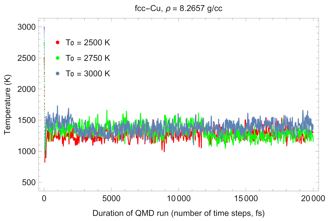
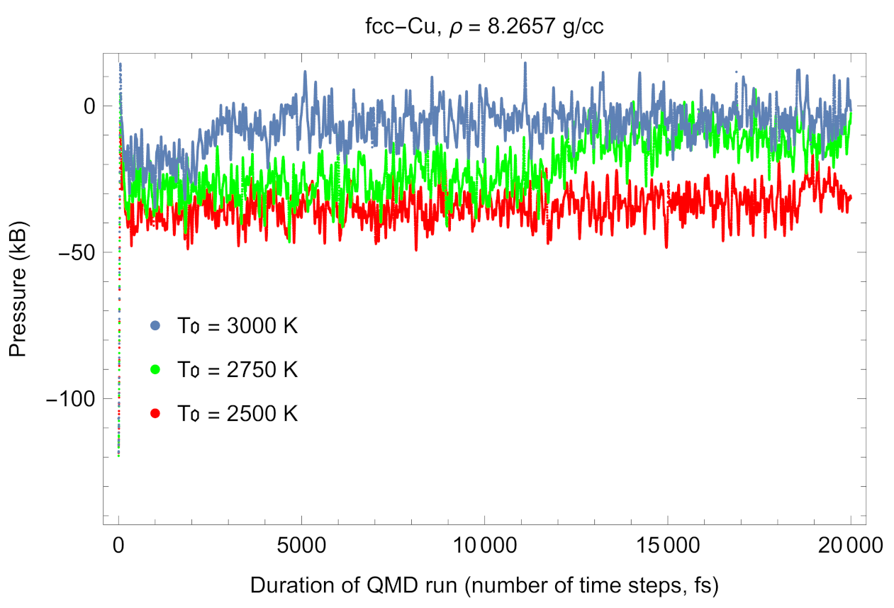
Figure 1, Figure 2, Figure 3 and Figure 4 offer two examples of our Z method melting simulations. They correspond to the first of the six s in each of the two cases, and show the time evolution of T and respectively, during the corresponding computer runs. Consider, for example, Figure 1 and Figure 2. During the K run, the system remains a superheated solid: both the average T and P stay virtually the same during the 20 ps of running time. The K run is the melting run [23], during which a melting occurs: it starts after ∼11 ps of running time, and the melting process takes about 2 ps. It results in the decrease of average T from ∼1400 to 1280 K, and the corresponding increase of average P from ∼−2 to −1.2 GPa. This is so because the total energy, is conserved, and V is fixed. For the same reason, Figure 1 and Figure 2, and Figure 3 and Figure 4 are “mirror images” of each other; see [23] for more detail. In the run with higher K, the melting starts after only 2 ps of running time, and the melting process takes only 1 ps. For a sufficiently high initial T, the system melts virtually immediately.
The results of our melting simulations are summarized in Table 1 and Table 2. The errors in melting T () are half of the increment of the initial T for a series of computer runs at the corresponding density [23]. We chose these increments to be 250 K for the 1st and 2nd, 500 K for the 3rd and 4th, 625 K for the 5th, and 750 K for the 6th in each of the two cases. The corresponding errors are listed in the tables as . The errors in melting P () are negligibly small, of the order 1–2 GPa in each case. Table 1 and Table 2 also include the values of that come from each of the thermal EOSs (1), (2) at the corresponding s.
The best fits to the corresponding six datapoints are the corresponding melting curves:
and
These fits are very accurate: the corresponding values of per d.o.f. are ≈1 for bcc-Cu, and ≈1.5 for fcc-Cu if is fixed at 1358 K, in agreement with the experiment, or otherwise ≈1, if it is considered as a free parameter; in the latter case, its value is ≈1357.9 K.
The first three terms of the power-series expansion of (3) are This is in good agreement with from the low-P experimental study of ref. [25]. Our value of at 40 K/GPa, is in the middle of the range of lower-P experiments: 44.5 [25], [26], 42 [27], 42 [28], 41.8 [29], 41 [30], [31], 36.4 [32]. The vast majority of the theoretical melting curves of fcc-Cu have similar values for the initial slope; e.g., 50 [33], 39 [34,35], 38 [36], 37.75 [37], 36.7 [38,39]. Ref. [39] does not offer an explicit value of at however, the Cu melting curve of [39] is virtually identical to that of [38].
At higher the melting curve of bcc-Cu is higher than that of fcc-Cu, therefore, bcc-Cu is thermodynamically more stable and represents the physical solid phase of copper. The melting curves cross each other at (P in GPa, T in K) , which is the fcc-bcc-liquid triple point. We note that our triple-point P-T coordinates are in excellent agreement with those from Ref. [16]: (80, 3490).
4. fcc-bcc Solid-Solid Phase Transition Boundary
Here we discuss the fcc-bcc solid–solid phase transition boundary in copper. We start our discussion with the derivation of a formula for the initial slope of a solid–solid phase transition boundary in general case.
4.1. Theoretical Estimate of the Initial Slope
Here, we derive a formula for the initial slope of a solid–solid phase transition boundary at the solid-solid-liquid triple point.
Let and be the volumes of, respectively, solid, solid and liquid at the solid-solid-liquid triple point, and and the corresponding entropies. According to the Clausius–Clapeyron formula, the slopes of the two melting curves at the triple point (where they cross each other) are
Then, the slope of the solid–solid phase transition boundary, also from the Clausius–Clapeyron formula and the above relations, is
where stands for volume change at melt of solid: The values of and come from the corresponding thermal EOSs, and those of and from the corresponding melting curve equations, at of the fcc-bcc-liquid triple point. Specifically, cm/mol, cm/mol (i.e., thus the phase boundary has a positive slope), and K/GPa and K/GPa. As the results of [40] show, by a pressure of 80–100 GPa, volume change at melt for fcc-Cu decreases by a factor of ∼2. The literature data on at span an interval of values from 0.045 [41] to 0.053 [42], or Hence, at the fcc-bcc-liquid triple point For our estimate of we assume that at the triple point Then, Equation (6) gives K/GPa. Thus, the initial slope of the fcc-bcc solid–solid phase boundary is ∼20 K/GPa. Now we can estimate the bcc-fcc entropy difference at the triple point: with the above values of and it follows from (6) that in good agreement with of Ref. [16].
4.2. Inverse-Z Simulations
Based on the above material of this work, we conclude that the the initial slope of the fcc-bcc solid–solid phase transition boundary is ∼20 K/GPa and that it is relatively flat. To further constrain the location of this boundary in the P-T plane, we carried out two sets of independent inverse Z runs (the inverse Z method is described in detail in [22]) to solidify liquid Cu and to check whether there is any solid–solid phase boundary so that liquid Cu solidifies into fcc on one side of this boundary and into bcc (or another solid structure) on the other side. We used a computational cell of 512 atoms prepared by melting a solid simple cubic (sc) supercell, which would eliminate any bias towards solidification into fcc or bcc, or any other solid structure. We used sc unit cells of 1.9446 and 1.8652 Å; the dimensions of bcc unit cells with the same volume as the sc ones are 2.45 and 2.35 Å, respectively, which corresponds to ∼200 and 360 GPa.
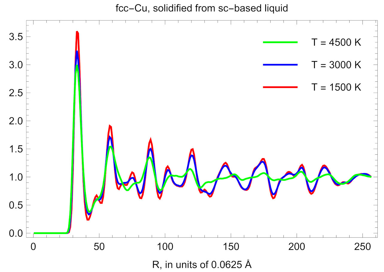
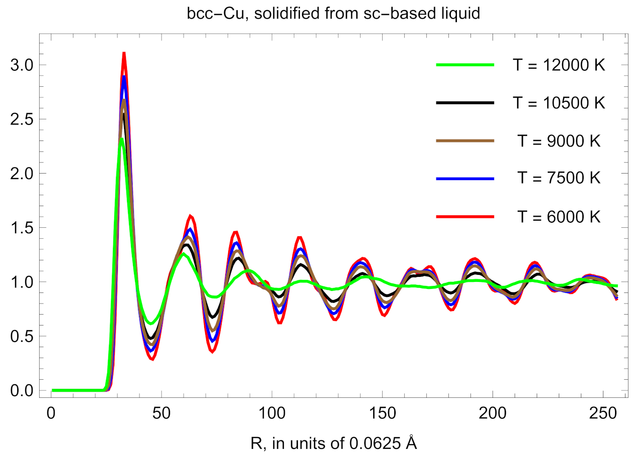
We carried out simulations using the Nosé–Hoover thermostat with a timestep of 1 fs. Complete solidification typically required from 15 to 25 ps, or 15,000–25,000 timesteps. The inverse Z runs indicate that in each case, liquid Cu solidifies into fcc below ∼5000 K and into bcc above ∼5000 K, so that the fcc-bcc transition boundary at high-P is relatively flat at ∼5000 K. The final states of the solidification were identified as fcc and bcc from analyzing the corresponding radial distribution functions (RDFs). RDFs of the final solid states are noisy; upon fast quenching of the two structures to low where RDFs are more discriminating, we could compare them to the RDFs of fcc and bcc and properly identify.
The RDFs of the solidified states at ∼400 GPa below the transition boundary are shown in Figure 5, and of those solidified above the transition boundary in Figure 6. The 4500 K state lies very close to the transition boundary. We assign it to fcc, because its short-range order (smaller-R) peaks are definitely fcc-like, while long-range order (larger-R) peaks are smeared and may somewhat resemble those of bcc in Figure 6. Most likely, this 4500 K state is some mixture of bcc and fcc, so it must be very close to the transition boundary or even lie on the boundary itself.
A few more comments are in order. The 12,000 K state at ∼500 GPa did not solidify, most likely for the reason of not being supercooled enough to initiate the solidification process [22]. Indeed, 12,000 K constitutes ∼0.92 of the corresponding of ∼13,050 K (i.e., 8% of supercooling), while for the solidification process to occur, a supercooling of at least 15% is needed [22]. For the other set of points at ∼250 GPa, the highest solidification T of 7000 K constitutes ∼0.83 of the corresponding of ∼8460 K (i.e., 17% of supercooling), which apparently allows for the solidification process to go through in this case.
5. Ab Initio Phase Diagram of Copper
Now we combine all the results of the previous sections of this work to construct the ab initio phase diagram of copper.
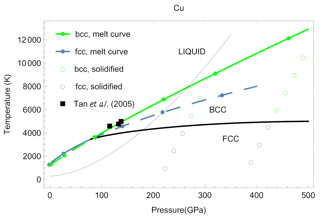
We take the P-T coordinates of the fcc-bcc-liquid triple point to be (79, 3460). A simple analytic form of the fcc-bcc solid–solid transition boundary which (i) crosses this triple point, (ii) has an initial slope of 19.9 K/GPa and (iii) takes into account the results of the inverse Z solidification simulations (i.e., to be between the 4500 K fcc and 6000 K bcc points at ∼260 GPa and to be close or even cross the 5000 K point at ∼430 GPa is
This phase boundary and the two melting curves (3) and (4) define the topology of our ab initio phase diagram of Cu shown in Figure 7. This phase diagram is topologically similar to the ab initio phase diagram of Smirnov [18], except that their melting curve of bcc-Cu seems to be the continuation of the melting curve of fcc-Cu to higher that is, the melting curve of Cu does not change its slope at the fcc-bcc-liquid triple point. The results of the previous section demonstrate that at the triple point the slope of the Cu melting curve increases by ∼20%, from 20.3 K/GPa on the fcc side to 25.9 K/GPa on the bcc side. The experimental conditions of Ref. [43] correspond to melting from bcc phase, and indeed, the three data points of [43] appear to lie on our bcc-Cu melting curve, see Figure 7.
Shown also in Figure 7 is the Cu principal Hugoniot obtained from fitting the numerical data of Ref. [44] with a simple analytic form:
This principal Hugoniot crosses the fcc-bcc phase transition boundary at = , in agreement with Ref. [11], which claims the bcc-fcc transition on the Hugoniot at 180 GPa. Furthermore, in Ref. [5], a distinct kink was detected in the Poisson ratio as a function of P at ∼185 GPa such that the Poisson ratio data were fitted with two different straight segments below and above the kink. In view of our findings, this kink is naturally explained as that corresponding to the fcc-bcc transition in Cu on its principal Hugoniot.
The Hugoniot melting point corresponds to the intersection of the bcc-Cu melting curve (4) and the above Hugoniot: in agreement with Ref. [5], which claims the melting on the Hugoniot at GPa.
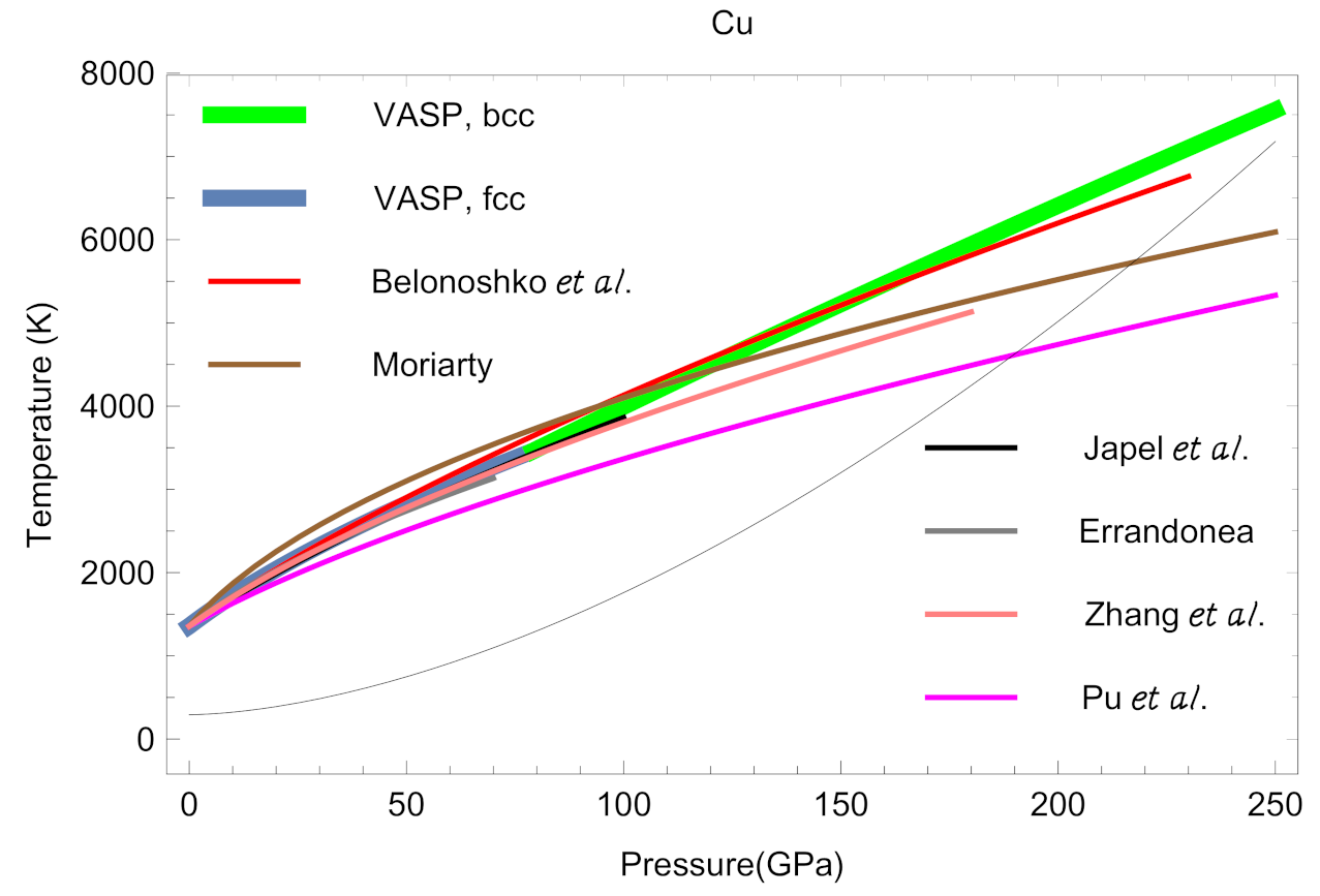
Figure 8 compares our ab initio melting curve of Cu to several melting curves among a few tens of those available in the literature, as it is not feasible to collect them all in one figure. Shown are the experimental melting curves of references [30,45] as well as the theoretical melting curves of refs. [38,40,46,47]. It is clearly seen that the best overall agreement of our melting curve of Cu, as a combination of both fcc and bcc segments, is with the theoretical melting curves of Belonoshko et al. [38] and Ghosh [39] which are virtually identical to each other. The reason for such a good agreement must be that in both [38,39] molecular dynamics simulations were done using embedded-atom model (EAM) for interatomic potentials, and the EAM parameters were obtained from fitting the model to ab initio data. It is interesting to note that in Ref. [43], their three experimental melting points are compared to the theoretical melting curve of [38], and excellent agreement is found. This fact provides mutual support to the validity of the experimental results of ref. [43] and to the computational methodologies of both Refs. [38,39] and the present study.
We note that the vast majority of the melting curves of fcc-Cu available in the literature converge to a unique analytic form similar to Equation (3). For example, in Figure 8, all the fcc-Cu melting curves except that of Ref. [40] can be effectively represented by that of ref. [47]. If only fcc-Cu were considered, the principal Hugoniot would have crossed it at ∼220 GPa, which would have been the P of the Hugoniot melting of Cu (). In fact, this is in agreement with several papers which all predicted GPa: –230 [17], –220 [48], and [49], to name just a few. In the latter work, the Hugoniot is 5560 K, in good agreement with 5843.0 from Equation (8).
6. Concluding Remarks
Let us now summarize the results of our theoretical study.
We have constructed the theoretical phase diagram of copper, using a suite of ab initio QMD simulations based on the Z methodology which combines both direct Z method for the simulation of melting curves and inverse Z method for the calculation of solid–solid phase boundaries. We determined that bcc-Cu becomes the thermodynamically stable solid structure of copper at high- and finds itself on the phase diagram of copper, along with fcc-Cu, its solid structure at ambient conditions. We have calculated the melting curves of both fcc-Cu and bcc-Cu, determined the location of the fcc-bcc-liquid triple point, and obtained an equation for the fcc-bcc solid–solid phase transition boundary. Last but not least, we have proposed thermal equations of state for both fcc-Cu and bcc-Cu, which appear to be in agreement with both experimental data and QMD simulations. Our theoretical phase diagram of copper represents the refinement of that of Smirnov for which the fcc-Cu and bcc-Cu melting curves as well as the fcc-bcc solid–solid phase boundary were estimated rather than being calculated using the DFT-based methodology as in the present work.
For a long time, copper has been considered both as a pressure and a shock-wave standard. It is worth dwelling on this point in light of our findings, which reaffirm the idea that copper is a multi-phase material that was put forward by Bolesta and Fomin [16,17] and confirmed in the subsequent experimental [11,12] and theoretical [18] studies.
As emphasized in [14], first-principles-based theoretical calculations do not find any other solid structure energetically competitive with fcc, at least to 10 TPa, and therefore Cu is not expected to undergo any P-induced structural phase transformations, which makes Cu an ideal choice as a pressure standard for all hydrostatic experiments expected in the near future, both isothermal and isentropic (ramp compression), in which T does not rise high enough to cross into the bcc-Cu phase stability region. In this respect, our thermal EOS of Cu, Equations (1) and (2), can be considered as an EOS standard.
The issue of Cu being a shock-wave standard deserves a somewhat more detailed discussion. Copper has been considered to be a reliable shock-wave standard because (i) it is a plastic material, so that the characteristics of its shock compression and static compression agree well with each other, (ii) when compressed, Cu has been supposed not to undergo any polymorphic transitions, and (iii) when melted, it undergoes a minor volume change, so that its shock compression characteristics change very little across the Hugoniot melting transition. Now, as it is firmly established, both experimentally and theoretically, that Cu is a polymorphic material, it is interesting to revisit the concept of Cu being a reliable shock-wave standard. First of all, the main shock-wave characteristics of a material depend on the values of a and b in the following (quasi)-linear relation between particle ( and shock () velocities along the Hugoniot: These values, in turn, depend on the parameters of the EOS [50]: As mentioned above, both fcc-Cu and bcc-Cu have very similar EOS parameters listed under Equation (1); in particular, the two values of a differ from each other by less than 0.5%. The two values of b are exactly the same. Hence, the shock-wave characteristics of both fcc-Cu and bcc-Cu are expected to be virtually identical to each other; in particular, T as a function of P along the Hugoniot should not change across the fcc-bcc transition, this is why Equation (8) was used as a common for both fcc and bcc. For this reason, experimental data on for both fcc-Cu and bcc-Cu should be described by a common straight segment instead of two different ones, which is very clearly seen in, e.g., Figure 3 of Ref. [14]; a deviation of from a single straight segment occurs at km/s which corresponds to GPa, above the Hugoniot melting point of 265 GPa; in other words, this deviation occurs in the P-T region of liquid Cu.
Thus, despite being a polymorphic material, both the thermal and shock-wave characteristics of two of its solid phases, fcc and bcc, are indeed virtually identical. This observation allow us to conclude that copper remains to be a reliable shock-wave standard, in addition to being reliable pressure calibrant and EOS standard.
Author Contributions
The authors contributed equally to this work. All authors have read and agreed to the published version of the manuscript.
Funding
This work was done under the auspices of the US DOE/NNSA. D.E. acknowledges financial support from Spanish Ministerio de Ciencia, Innovación y Universidades (Grants Nos. PID2019-106383GB-C41 and RED2018-102612-T), and Generalitat Valenciana (Prometeo/2018/123 EFIMAT).
Data Availability Statement
All relevant data that support the findings of this study are available from the corresponding author upon request.
Acknowledgments
The QMD simulations were performed on the LANL cluster Badger as part of the Institutional Computing project w20phadiagurox.
Conflicts of Interest
The authors declare no conflict of interest.
References
- Meyers, M.A.; Gregori, F.; Kad, B.K.; Schneider, M.S.; Kalantar, D.H.; Remington, B.A.; Ravichandran, G.; Boehly, T.; Wark, J.S. Laser-induced shock compression of monocrystalline copper: Characterization and analysis. Acta Mater. 2003, 51, 1211–1228. [Google Scholar] [CrossRef]
- Murphy, W.J.; Higginbotham, A.; Kimminau, G.; Barbrel, B.; Bringa, E.M.; Hawreliak, J.; Kodama, R.; Koenig, M.; McBarron, W.; Meyers, M.A.; et al. The strength of single crystal copper under uniaxial shock compression at 100 GPa. J. Phys. Cond. Mat. 2010, 22, 065404. [Google Scholar] [CrossRef] [PubMed]
- Kraus, R.G.; Davis, J.P.; Seagle, C.T.; Fratuono, D.E.; Swift, D.C.; Brown, J.L.; Eggert, J.H. Dynamic compression of copper to over 450 GPa: A high-pressure standard. Phys. Rev. B 2016, 93, 134105. [Google Scholar] [CrossRef] [Green Version]
- Bell, P.M.; Xu, J.A.; Mao, H.K. Static compression of gold and copper and calibration of the ruby pressure scale to pressures to 1.8 megabars (static. RNO). In Shock Waves in Condensed Matter; Springer: Boston, MA, USA, 1986; pp. 125–130. [Google Scholar]
- Hayes, D.; Hixson, R.S.; McQueen, R.G. High pressure elastic properties, solid–liquid phase boundary and liquid equation of state from release wave measurements in shock-loaded copper. AIP Conf. Proc. 2000, 505, 483. [Google Scholar]
- Fratanduono, D.E.; Smith, R.F.; Ali, S.J.; Braun, D.G.; Fernandez-Pañella, A.; Zhang, S.; Kraus, R.G.; Coppari, F.; McNaney, J.M.; Marshall, M.C.; et al. Probing the solid phase of noble metal copper at terapascal conditions. Phys. Rev. Lett. 2020, 124, 015701. [Google Scholar] [CrossRef] [PubMed]
- Wang, L.G.; Šob, M. Structural stability of higher-energy phases and its relation to the atomic configurations of extended defects: The example of Cu. Phys. Rev. B 1999, 60, 844. [Google Scholar] [CrossRef]
- Friedel, J. On the stability of the body centred cubic phase in metals at high temperatures. J. Physique Lett. 1974, 35, 59–63. [Google Scholar] [CrossRef]
- Anupam, N.; Mitra, N. A metastable phase of shocked bulk single crystal copper: An atomistic simulation study. Sci. Rep. 2017, 7, 7337. [Google Scholar]
- Sims, M.; Briggs, R.; Coppari, F.; Coleman, A.L.; Gorman, M.G.; Panella-Fernandez, A.; Smith, R.F.; Eggert, J.H.; Wicks, J.K. Copper phase determination to 290 GPa using laser-shock compression. In Proceedings of the 2019 COMPRES Annual Meeting, Big Sky Resort, Big Sky, MT, USA, 2–5 August 2019. [Google Scholar]
- Sharma, S.M.; Turneaure, S.J.; Winey, J.M.; Gupta, Y.M. Transformation of shock-compressed copper to the body-centered-cubic structure at 180 GPa. Phys. Rev. B 2020, 102, 020103. [Google Scholar] [CrossRef]
- Mei, W.; Wen, Y.; Xing, H.; Ou, P.; Sun, J. Ab initio calculations of mechanical stability of bcc Cu under pressure. Solid State Commun. 2014, 184, 25. [Google Scholar] [CrossRef]
- Xiong, Q.; Kitamura, T.; Li, Z. Transient phase transitions in single-crystal coppers under ultrafast lasers induced shock compression: A molecular dynamics study. J. Appl. Phys. 2019, 125, 194302. [Google Scholar] [CrossRef]
- Greeff, C.W.; Boettger, J.C.; Graf, M.J.; Johnson, J.D. Theoretical investigation of the Cu EOS standard. J. Phys. Chem. Solids 2006, 67, 2033. [Google Scholar] [CrossRef]
- Errandonea, D.; Burakovsky, L.; Preston, D.L.; MacLeod, S.G.; Santamaría-Perez, D.; Chen, S.; Cynn, H.; Simak, S.I.; McMahon, M.I.; Proctor, J.E.; et al. Experimental and theoretical confirmation of an orthorhombic phase transition in niobium at high pressure and temperature. Commun. Mater. 2020, 1, 60. [Google Scholar] [CrossRef]
- Bolesta, A.V.; Fomin, V.M. Molecular dynamics simulation of shock-wave loading of copper and titanium. AIP Conf. Proc. 2017, 1893, 020008. [Google Scholar]
- Bolesta, A.V.; Fomin, V.M. Molecular dynamics simulations of polycrystalline copper. J. Appl. Mech. Tech. Phys. 2014, 55, 800. [Google Scholar] [CrossRef]
- Smirnov, N.A. Relative stability of Cu, Ag, and Pt at high pressures and temperatures from ab initio calculations. Phys. Rev. B 2021, 103, 064107. [Google Scholar] [CrossRef]
- Wallace, D.C. Statistical Physics of Crystals and Liquids; World Scientific: Singapore, 2002; p. 191. [Google Scholar]
- Dewaele, A.; Loubeyre, P.; Mezouar, M. Equations of state of six metals above 94 GPa. Phys. Rev. B 2004, 70, 094112. [Google Scholar] [CrossRef] [Green Version]
- Zinov’ev, V.E. Handbook of Thermophysical Properties of Metals at High Temperatures; Nova Science Publishers: New York, NY, USA, 1996; p. 95. [Google Scholar]
- Burakovsky, L.; Chen, S.P.; Preston, D.L.; Sheppard, D.G. Z methodology for phase diagram studies: Platinum and tantalum as examples. J. Phys. Conf. Ser. 2014, 500, 162001. [Google Scholar] [CrossRef] [Green Version]
- Burakovsky, L.; Burakovsky, N.; Preston, D.L. Ab initio melting curve of osmium. Phys. Rev. B 2015, 92, 174105. [Google Scholar] [CrossRef] [Green Version]
- Belonoshko, A.B.; Skorodumova, N.V.; Rosengren, A.; Johansson, B. Melting and critical superheating. Phys. Rev. B 2006, 73, 012201. [Google Scholar] [CrossRef]
- Brand, H.; Dobson, D.P.; Vočadlo, L.; Wood, I.G. Melting curve of copper measured to 16 GPa using a multi-anvil press. High Pres. Res. 2006, 26, 185. [Google Scholar] [CrossRef]
- Errandonea, D. The melting curve of ten metals up to 12 GPa and 1600 K. J. Appl. Phys. 2010, 108, 033517. [Google Scholar] [CrossRef]
- Butuzov, V.P. The investigation of phase transformations as superhigh pressures. Kristallografiya 1957, 2, 536. [Google Scholar]
- Mitra, N.R.; Decker, D.L.; Vanfleet, H.B. Melting Curves of Copper, Silver, Gold, and Platinum to 70 kbar. Phys. Rev. 1967, 161, 613. [Google Scholar] [CrossRef]
- Mirwald, P.; Kennedy, G.C. The melting curve of gold, silver, and copper to 60-kbar pressure: A reinvestigation. J. Geophys. Res. 1979, 84, 6750. [Google Scholar] [CrossRef]
- Errandonea, D. High-pressure melting curves of the transition metals Cu, Ni, Pd, and Pt. Phys. Rev. B 2013, 87, 054108. [Google Scholar] [CrossRef]
- Cohen, L.M.; Klement, W.; Kennedy, G.C. Melting of Copper, Silver, and Gold at High Pressures. Phys. Rev. 1966, 145, 519. [Google Scholar] [CrossRef]
- Akella, J.; Kennedy, G.C. Melting of Gold, Silver, and Copper - Proposal for a New High-Pressure Calibration Scale. J. Geophys. Res. 1971, 76, 4969. [Google Scholar] [CrossRef]
- Górecki, T. Vacancies and a generalised melting curve of metals. High Temp. High Press. 1979, 11, 683. [Google Scholar]
- Tam, P.D.; Tan, P.D.; Hoc, N.Q.; Phong, P.D. Melting of matals copper, silver and gold under pressure. Proc. Nat. Conf. Theor. Phys. 2010, 35, 148. [Google Scholar]
- Tam, P.D.; Hoc, N.Q.; Tinh, B.D.; Tan, P.D. Melting curve of metals Cu, Ag and Au under pressure. Mod. Phys. Lett. B 2016, 30, 1550273. [Google Scholar] [CrossRef]
- Vočadlo, L.; Alfè, D.; Price, G.D.; Gillan, M.J. Ab initio melting curve of copper by the phase coexistence approach. J. Chem. Phys. 2004, 120, 2872. [Google Scholar] [CrossRef] [PubMed]
- Mazhukin, V.I.; Demin, M.M.; Aleksashkina, A.A. Atomistic modeling of thermophysical properties of copper in the region of the melting point. Math. Montisnigri 2018, 41, 99. [Google Scholar]
- Belonoshko, A.B.; Ahuja, R.; Eriksson, O.; Johansson, B. Quasi ab initio molecular dynamic study of Cu melting. Phys. Rev. B 2000, 61, 3838. [Google Scholar] [CrossRef]
- Ghosh, K. Melting curve of metals using classical molecular dynamics simulations. J. Phys. Conf. Ser. 2012, 377, 012085. [Google Scholar] [CrossRef] [Green Version]
- Pu, C.; Yang, X.; Xiao, D.; Cheng, J. Molecular dynamics simulations of shock melting in single crystal Al and Cu along the principle Hugoniot. Mater. Today Commun. 2021, 26, 101990. [Google Scholar] [CrossRef]
- Cahill, J.A.; Kirshenbaum, A.D. The density of liquid copper from its melting point (1356 ∘K) to 2500 ∘K. Furthermore, an estimate of its critical constants. J. Phys. Chem. 1962, 66, 1080. [Google Scholar] [CrossRef]
- Blumm, J.; Henderson, J.B. Measurement of the volumetric expansion and bulk density of metals in the solid and molten regions. High Temp. High Press. 2000, 32, 109. [Google Scholar] [CrossRef]
- Tan, H.; Dai, C.D.; Zhang, L.Y.; Xu, C.H. Method to determine the melting temperatures of metals under megabar shock pressures. Appl. Phys. Lett. 2005, 87, 221905. [Google Scholar] [CrossRef]
- Kinslow, R. (Ed.) High-Velocity Impact Phenomena; Academic Press: New York, NY, USA, 1970; p. 532. [Google Scholar]
- Japel, S.; Schwager, B.; Boehler, R.; Ross, M. Melting of copper and nickel at high rressure: The role of d electrons. Phys. Rev. Lett. 2005, 95, 167801. [Google Scholar] [CrossRef]
- Moriarty, J.A. High-pressure ion-thermal properties of metals from ab initio interatomic potentials. In Shock Waves in Condensed Matter, Gupta, Y.M., Ed.; Plenum Press: New York, NY, USA, 1986. [Google Scholar]
- Zhang, B.; Wang, B.; Liu, Q. Melting curves of Cu, Pt, Pd and Au under high pressures. Int. J. Mod. Phys. B 2016, 30, 1650013. [Google Scholar] [CrossRef]
- Bringa, E.M.; Cazamias, J.U.; Erhart, P.; Stölken, J.; Tanushev, N.; Wirth, B.D.; Rudd, R.E.; Caturla, M.J. Atomistic shock Hugoniot simulation of single-crystal copper. J. Appl. Phys. 2004, 96, 3793. [Google Scholar] [CrossRef] [Green Version]
- Gubin, S.A.; Maklashova, I.V.; Mel’nikov, I.N. The Hugoniot adiabat of crystalline copper based on molecular dynamics simulation and semiempirical equation of state. J. Phys. Conf. Ser. 2018, 946, 012098. [Google Scholar] [CrossRef]
- Johnson, J.D. The features of the principal Hugoniot. AIP Conf. Proc. 1998, 429, 27. [Google Scholar]
Figure 1.
The melting point of fcc-Cu at a density of 8.2627 g/cc: melting T from ab initio Z method implemented with VASP.
Figure 1.
The melting point of fcc-Cu at a density of 8.2627 g/cc: melting T from ab initio Z method implemented with VASP.

Figure 2.
The same as in Figure 1 for melting
Figure 2.
The same as in Figure 1 for melting

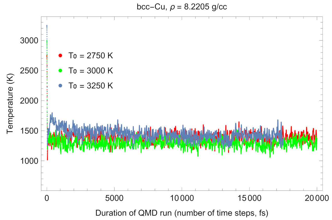
Figure 3.
The same as in Figure 1 for bcc-Cu at a density of 8.2205 g/cc.
Figure 3.
The same as in Figure 1 for bcc-Cu at a density of 8.2205 g/cc.

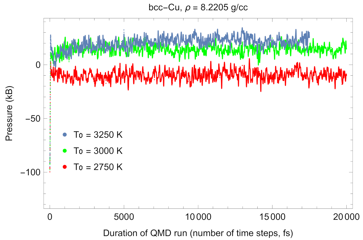
Figure 4.
The same as in Figure 3 for melting
Figure 4.
The same as in Figure 3 for melting

Figure 5.
Radial distribution functions (RDFs) of the final states of the solidification of liquid Cu at ∼400 GPa at lower temperatures.
Figure 5.
Radial distribution functions (RDFs) of the final states of the solidification of liquid Cu at ∼400 GPa at lower temperatures.

Figure 6.
Radial distribution functions (RDFs) of the final states of the solidification of liquid Cu at ∼400 GPa at higher temperatures.
Figure 6.
Radial distribution functions (RDFs) of the final states of the solidification of liquid Cu at ∼400 GPa at higher temperatures.

Figure 7.
The ab initio phase diagram of Cu. Three experimental points (filled circles) are from ref. [43]. The fcc-bcc solid–solid phase transition boundary (black curve) is estimated based on the results of the inverse Z method simulations of the solidification of liquid Cu into fcc and bcc solid structures on other sides of the boundary. The principal Hugoniot of Cu is also shown as a thin black curve.

Figure 8.
Comparison of the ab initio melting curve of Cu calculated in this work (which combines both lower-P fcc and higher-P bcc segments) to several melting curves of Cu available in the literature: Errandonea [30], Belonoshko [38], Pu et al. [40], Japel et al. [45], Moriarty [46], and Zhang et al. [47]. The Cu principal Hugoniot is also shown as a thin black line.


Table 1.
The six ab initio melting points of fcc-Cu, obtained from the Z method implemented with VASP.
Table 1.
The six ab initio melting points of fcc-Cu, obtained from the Z method implemented with VASP.
| Lattice Constant (Å) | Density (g/cm) | (GPa) | from (1), (2) | (K) | (K) |
|---|---|---|---|---|---|
| 3.71 | 8.2657 | −1.20 | −1.453 | 1280 | 125.0 |
| 3.51 | 9.7607 | 26.5 | 26.45 | 2220 | 125.0 |
| 3.31 | 11.639 | 87.4 | 87.35 | 3620 | 250.0 |
| 3.21 | 12.761 | 140 | 140.5 | 4570 | 250.0 |
| 3.11 | 14.032 | 218 | 218.5 | 5780 | 312.5 |
| 3.01 | 15.478 | 333 | 332.9 | 7230 | 375.0 |
Table 2.
The six ab initio melting points of bcc-Cu, obtained from the Z method implemented with VASP.
Table 2.
The six ab initio melting points of bcc-Cu, obtained from the Z method implemented with VASP.
| Lattice Constant (Å) | Density (g/cm) | (GPa) | from (1), (2) | (K) | (K) |
|---|---|---|---|---|---|
| 2.95 | 8.2205 | 1.42 | 1.363 | 1290 | 125.0 |
| 2.80 | 9.6138 | 27.8 | 27.78 | 2070 | 125.0 |
| 2.65 | 11.341 | 85.9 | 85.97 | 3640 | 250.0 |
| 2.49 | 13.670 | 220 | 219.8 | 6880 | 250.0 |
| 2.42 | 14.891 | 320 | 320.2 | 9110 | 312.5 |
| 2.35 | 16.262 | 462 | 461.8 | 12,130 | 375.0 |
Publisher’s Note: MDPI stays neutral with regard to jurisdictional claims in published maps and institutional affiliations. |
© 2021 by the authors. Licensee MDPI, Basel, Switzerland. This article is an open access article distributed under the terms and conditions of the Creative Commons Attribution (CC BY) license (https://creativecommons.org/licenses/by/4.0/).
Share and Cite
MDPI and ACS Style
Baty, S.R.; Burakovsky, L.; Errandonea, D. Ab Initio Phase Diagram of Copper. Crystals 2021, 11, 537. https://doi.org/10.3390/cryst11050537
AMA Style
Baty SR, Burakovsky L, Errandonea D. Ab Initio Phase Diagram of Copper. Crystals. 2021; 11(5):537. https://doi.org/10.3390/cryst11050537
Chicago/Turabian StyleBaty, Samuel R., Leonid Burakovsky, and Daniel Errandonea. 2021. "Ab Initio Phase Diagram of Copper" Crystals 11, no. 5: 537. https://doi.org/10.3390/cryst11050537
Note that from the first issue of 2016, this journal uses article numbers instead of page numbers. See further details here.