Diagonalization Method to Hyperbolic Two-Temperature Generalized Thermoelastic Solid Sphere under Mechanical Damage Effect

Abstract

This study is the first to use the diagonalization method for the new modelling of a homogeneous, thermoelastic, and isotropic solid sphere that has been subjected to mechanical damage. The fundamental equations were derived using the hyperbolic two-temperature generalized thermoelasticity theory with mechanical damage taken into account. The outer surface of the sphere has been assumed to have been shocked thermally without cubical dilatation. The numerical results for the dynamical and conductive temperatures increment, strain, displacement, and average of the principal stresses components have been represented graphically with different values of the hyperbolic two-temperature parameter and mechanical damage parameters. The two-temperature model parameter and the mechanical damage parameter have significant effects. The propagations of the thermomechanical waves take place at finite speeds in the context of the hyperbolic two-temperature theory as well as in the usual context of the Lord–Shulman theory with one-temperature.

1. Introduction

Several mathematical models for heat transport and thermal waves in solids and thermoelastic materials have been created by researchers. However, not all of these models are accurate because obtaining a finite progress rate of mechanical and thermal waves for the experimental effects is one of the best model parameters. We will look at experimental models that are close to laboratory findings and that are consistent with the physical behavior of thermoelastic material as well as try to include new information.

Chen and Gurtin proposed the thermoelasticity theory based on two different temperatures: conductive and dynamic temperatures. Differences are according to the amount of heat supply between these two types of temperatures [1]. Warren and Chen looked at how waves propagate under the notion of a two-temperature framework [2]. However, this hypothesis did not change until Youssef modified this hypothesis and presented the two-temperature model of general thermoelasticity [3]. Youssef co-operated with other authors and used this model in many applications [4,5,6]. Youssef and El-Bary reported that the classical generalized two-temperature thermoelectricity model does not provide a given speed of thermal wave propagation [7]. This model was then modified by Youssef and El-Bary and was developed into a new two-temperature model based on the various laws of heat conduction, which are known as generalized hyperbolic two-temperature thermoelasticity [7,8,9]. Youssef suggested the difference between the conductive temperature acceleration and the dynamic temperature acceleration during the material transition is proportional to the heat supply. Within this model, the speed of thermal wave propagation is reduced [7]. Hobiny [10] applied the hyperbolic two-temperature model without dissipating the energy on the photothermal interaction in a semiconducting medium. Alshehri and Lotfy studied a theoretical novel model of generalized photo-thermoelasticity and a hyperbolic two-temperature theory [11]. Abbas et al. investigated photo–thermal–elastic interactions in an unbounded semiconductor media containing a cylindrical hole under a hyperbolic two-temperature model [12]. Youssef solved some applications of an infinite thermoelastic spherical medium subjected to a moving heat source, fractional strain, rotation, and mechanical damage [13,14,15].

For the isotropic damage, the total effective stresses takes the form [16]:

$${\sigma }_{ij}=\left(1-D\right){\tilde{\sigma }}_{ij}$$

(1)

where in the undamaged material, ${\tilde{\sigma }}_{ij}$ are the stress tensor components. The variable of mechanical damage may be represented in many ways. We consider an area element $dA$ with unit normal vector n in a cross-section of the damaged body. Hence, the area of the defects in this element is given by $d{A}_D$, and the total amount of the damage $D$ can be obtained by the area fraction as follows [16]:

$$D=\frac{d{A}_D}{dA}, 0\le D\le 1$$

(2)

Hence, $D=0$ represents the undamaged material, and $D=1$ formally represents the complete full damage of the material. In real materials, processes take place at values $D\approx 0.2\dots 0.5$.

The description of the damage mechanics in Equation (2) has been published in many applications and models [17,18,19,20,21].

This work aims to study and discuss the effects of the mechanical damage parameters on the induced conductive temperature, dynamic temperature, deformation, and stress fields in a thermoelastic solid sphere by using the diagonalization method for the first time. The governing equations of the mathematical model have been prepared by using the hyperbolic two-temperature heat conduction theory when the mechanical damage variable is included.

2. The Governing Equations

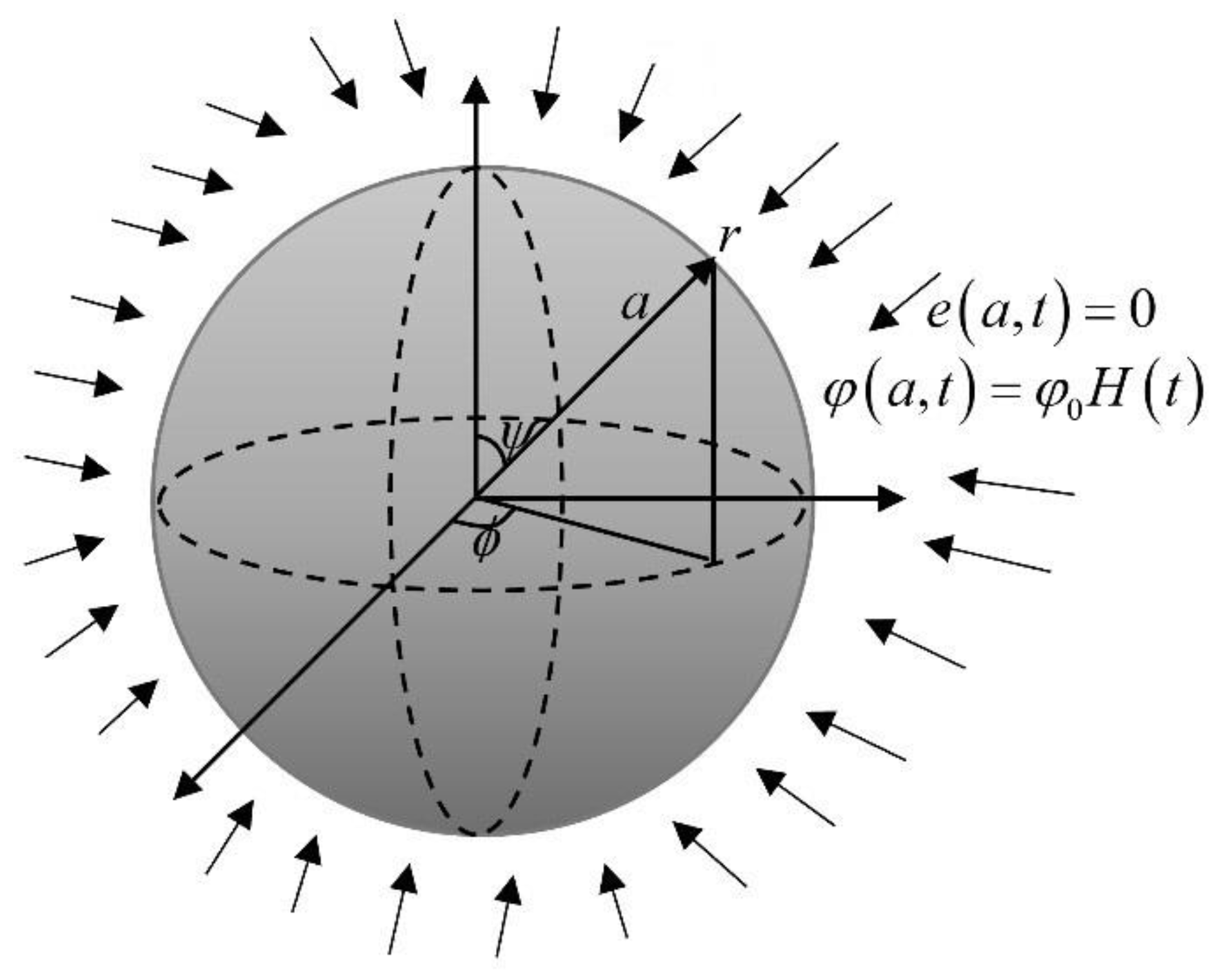
Consider a perfect conducting, isotropic, and thermoelastic spherical body that fills the region $\mathsf{\Lambda }=\left\{\left(r,\psi ,\varphi \right): 0\le r\le a, 0\le \psi \le 2\pi , 0\le \varphi <2\pi \right\}$. We use the spherical coordinates system $\left(r,\psi ,\varphi \right)$, where $r$ denotes the radial co-ordinate, $\psi$ denotes the co-latitude, and $\varphi$ indicates the longitude of a spherical coordinate system, respectively, as seen in Figure 1. We assume the sum of the external forces is zero and that it is initially quiescent. Only when there are no latitudinal and longitudinal differences in the symmetry is the requirement fulfilled. All state functions will therefore be dependent on the radial distance r and time t.

Because of the spherical symmetry, the components of displacement take the form:

$$U\left(r,t\right)=\left(u\left(r,t\right),0,0 \right)$$

(3)

The essential equation of motion is

$$\left(\lambda +2\mu \right)\left(1-D\right)\frac{\partial e}{\partial r}-\gamma \left(1-D\right)\frac{\partial T_D}{\partial r}=\rho \ddot{u}$$

(4)

The constitutive equations with the damage mechanics variable are

$${\sigma }_{rr}=2\left(1-D\right)\mu e_{rr}+\lambda \left(1-D\right)e-\gamma \left(1-D\right)\left(T_D-T_0\right)$$

(5)

$${\sigma }_{\psi \psi }=2\mu \left(1-D\right)e_{\psi \psi }+\lambda \left(1-D\right)e-\gamma \left(1-D\right)\left(T_D-T_0\right)$$

(6)

$${\sigma }_{\varphi \varphi }=2\mu \left(1-D\right)e_{\varphi \varphi }+\lambda \left(1-D\right)e-\gamma \left(1-D\right)\left(T_D-T_0\right)$$

(7)

$${\sigma }_{r\varphi }= {\sigma }_{\varphi \psi }={\sigma }_{r\psi }=0$$

(8)

The strain components are

$$e_{rr}=\frac{\partial u}{\partial r}, e_{\psi \psi }=e_{\varphi \varphi }=\frac{u}{r}$$

(9)

and

$$e_{r\varphi }=e_{\varphi \psi }= e_{r\psi }=0$$

(10)

$e$ defines the cubical dilatation and satisfies the relation

$$e=e_{rr}+e_{\psi \psi }+e_{\varphi \varphi }=\frac{\partial u}{\partial r}+\frac{2u}{r}=\frac{1}{r^2}\frac{\partial \left(r^{2}u\right)}{\partial r}$$

(11)

The heat conduction equation under the hyperbolic two-temperature theory takes the forms

$$K{\nabla }^2{T}_C=\left(\frac{\partial }{\partial t}+{\tau }_0\frac{\partial { }^2}{\partial t^2}\right)\left[ \rho C_E{T}_D+ \gamma T_{0}e\right]$$

(12)

and

$${\ddot{T}}_C-{\ddot{T}}_D=c^2{\nabla }^2{T}_C$$

(13)

$c\left(m s^{-1}\right)$ is called the parameter of the hyperbolic two-temperature theory, and ${\nabla }^2=\frac{1}{r^2}\frac{\partial }{\partial r}\left(r^2\frac{\partial }{\partial r}\right)$.

We assume that $\phi =\left(T_C-T_0\right)$ and $\theta =\left(T_D-T_0\right)$, where $\phi$ is the conductive temperature increment while $\theta$ is the dynamic temperature increment. Hence, Equations (4)–(7), (12), and (13) take the forms

$$\left(1-D\right)\left[\left(\lambda +2\mu \right)\frac{\partial e}{\partial r}-\gamma \frac{\partial \theta }{\partial r}\right]=\rho \ddot{u}$$

(14)

$${\sigma }_{rr}=\left(1-D\right)\left[2\mu e_{rr}+\lambda e-\gamma \theta \right]$$

(15)

$${\sigma }_{\psi \psi }=\left(1-D\right)\left[2\mu e_{\psi \psi }+\lambda e-\gamma \theta \right]$$

(16)

$${\sigma }_{\varphi \varphi }=\left(1-D\right)\left[2\mu e_{\varphi \varphi }+\lambda e-\gamma \theta \right]$$

(17)

Equation (14) can be modified to be in the form

$$\left(1-D\right)\left[\left(\lambda +2\mu \right){\nabla }^{2}e-\gamma {\nabla }^2\theta \right]=\rho \ddot{e}$$

(18)

To simplify the equations, we will use the following dimensionless variables [5,22]:

$$\left\{t^{\prime },{\tau }^{\prime },{{\tau }^{\prime }}_o\right\}=c_o^2\eta \left\{t,\tau ,{\tau }_o\right\}, \left\{r^{\prime },u^{\prime },a^{\prime }\right\}=c_o\eta \left\{r,u,a\right\}, \left\{{\theta }^{\prime },{\phi }^{\prime }\right\}=\frac{1}{T_0}\left\{\theta ,\phi \right\}, {\sigma }^{\prime }=\frac{\sigma }{\mu }$$

(19)

We then obtain

$$\left(1-D\right) \left[{\nabla }^{2}e-b{\nabla }^2\theta \right] =\ddot{e}$$

(20)

$${\nabla }^2\phi =\left(\frac{\partial }{\partial t}+{\tau }_o\frac{\partial { }^2}{\partial t^2}\right) \left[\theta + \epsilon e\right]$$

(21)

$$\ddot{\phi }-\ddot{\theta }={\tilde{c}}^2{\nabla }^2\phi$$

(22)

$${\sigma }_{rr}= \left(1-D\right)\left[{\beta }^{2}e-2\frac{u}{r}-{\epsilon }_1 \theta \right]$$

(23)

$${\sigma }_{\psi \psi }=\left(1-D\right)\left[{\beta }^{2}e-2\frac{\partial u}{\partial r}-{\epsilon }_1 \theta \right]$$

(24)

$${\sigma }_{\varphi \varphi }=\left(1-D\right)\left[{\beta }^{2}e-2\frac{\partial u}{\partial r}-{\epsilon }_1 \theta \right]$$

(25)

where $\gamma =\left(3\lambda +2\mu \right) {\alpha }_T$, $c_o^2=\frac{\lambda +2\mu }{\rho }$, $\eta =\frac{\rho C_E}{K}$, $\epsilon =\frac{\gamma }{\rho C_E}$, ${\epsilon }_1=\frac{\gamma T_o}{\mu }$, $\beta ={\left(\frac{\lambda +2\mu }{\mu }\right)}^{\raisebox{1ex}{$1$}\!\left/ \!\raisebox{-1ex}{$2$}\right.}$, $b=\frac{{\epsilon }_1}{{\beta }^2}$, ${\tilde{c}}^2=\frac{c^2}{c_o^2}$.

The primes have been deleted for simplicity.

The differential operator ${\nabla }^2=\frac{1}{r^2}\frac{\partial }{\partial r}\left(r^2\frac{\partial }{\partial r}\right)$ is a singular operator when $r=0$, and this singularity could be removed by applying L’Hopital’s rule as follows [23]:

$${\nabla }^2\left\{e,\theta ,\phi \right\}=\underset{r\to 0}{\lim }\left[\frac{1}{r^2}\frac{\partial }{\partial r}\left(r^2\frac{\partial \left\{e,\theta ,\phi \right\}}{\partial r}\right)\right]=\underset{r\to 0}{\lim }\left[\frac{{\partial }^2\left\{e,\theta ,\phi \right\}}{\partial r^2}+\frac{2}{r}\frac{\partial \left\{e,\theta ,\phi \right\}}{\partial r}\right]=\frac{{\partial }^2\left\{e,\theta ,\phi \right\}}{\partial r^2}+2\frac{{\partial }^2\left\{e,\theta ,\phi \right\}}{\partial r^2}$$

We then acquire

$${\nabla }^2\left\{e,\theta ,\phi \right\}=3\frac{{\partial }^2}{\partial r^2} \left\{e,\theta ,\phi \right\}$$

(26)

and satisfy the boundary conditions

$${\frac{\partial }{\partial r}\left\{e,\theta ,\phi \right\}|}_{r=0}=0$$

(27)

We then obtain

$${\nabla }^{2}e\left(r,t\right)=3\frac{{\partial }^{2}e\left(r,t\right)}{\partial r^2}, {\nabla }^2\theta \left(r,t\right)=3\frac{{\partial }^2\theta \left(r,t\right)}{\partial r^2}, {\nabla }^2\phi \left(r,t\right)=3\frac{{\partial }^2\phi \left(r,t\right)}{\partial r^2}$$

(28)

By using the forms in Equation (26) in Equations (20)–(22), we obtain the following equations:

$$3\left(1-D\right) \frac{{\partial }^{2}e}{\partial r^2}-3b\left(1-D\right)\frac{{\partial }^2\theta }{\partial r^2} =\ddot{e}$$

(29)

$$3\frac{{\partial }^2\phi }{\partial r^2}=\left(\frac{\partial }{\partial t}+{\tau }_o\frac{\partial { }^2}{\partial t^2}\right) \left[\theta + \epsilon e\right]$$

(30)

$$\ddot{\phi }-\ddot{\theta }=3{\tilde{c}}^2\frac{{\partial }^2\phi }{\partial r^2}$$

(31)

The Laplace transform is applied as follows:

$$\ell \left\{f\left(r,t\right)\right\}=\overline{f}\left(r,s\right)={\displaystyle {\int }_0^{\infty }{e}^{-st}f\left(r,t\right) dt}$$

(32)

when the following zero initial conditions have been used:

$$e\left(r,0\right)=\phi \left(r,0\right)=\theta \left(r,0\right)={\frac{\partial e\left(r,t\right)}{\partial t}|}_{t=0}={\frac{\partial \theta \left(r,t\right)}{\partial t}|}_{t=0}={\frac{\partial \phi \left(r,t\right)}{\partial t}|}_{t=0}=0$$

(33)

Equations (20)–(25) then take the following forms:

$$\left(1-D\right)\left[3 \frac{d^2\overline{e}}{d{r}^2}-3b\frac{d^2\overline{\theta }}{d{r}^2} \right]=s^2\overline{e}$$

(34)

$$3\frac{d^2\overline{\phi }}{d{r}^2}=\left(s+{\tau }_0{s}^2\right) \left[\overline{\theta }+ \epsilon \overline{e}\right]$$

(35)

$$\overline{\theta }=\overline{\phi }-{\delta }^2\frac{d^2\overline{\phi }}{d{r}^2}$$

(36)

$${\overline{\sigma }}_{rr}= \left(1-D\right)\left[{\beta }^2\overline{e}-2\frac{\overline{u}}{r}-{\epsilon }_1 \overline{\theta }\right]$$

(37)

$${\overline{\sigma }}_{\psi \psi }=\left(1-D\right)\left[{\beta }^2\overline{e}-2\frac{d \overline{u}}{d r}-{\epsilon }_1\overline{\theta }\right]$$

(38)

$${\overline{\sigma }}_{\varphi \varphi }=\left(1-D\right)\left[{\beta }^2\overline{e}-2\frac{d \overline{u}}{d r}-{\epsilon }_1\overline{\theta }\right]$$

(39)

$$\overline{e}=\frac{1}{r^2}\frac{d\left(r^2\overline{u}\right)}{dr}$$

(40)

where ${\delta }^2=\frac{3{\tilde{c}}^2}{s^2}$.

Using Equation (36) and Equations (34) and (35), we obtain

$$\left(\frac{d^2}{d{r}^2}-{\alpha }_1\right)\overline{e}=b\frac{d^2\overline{\phi }}{d{r}^2} -b{\delta }^2\frac{d^4\overline{\phi }}{d{r}^4}$$

(41)

$$\frac{d^2\overline{\phi }}{d{r}^2}= {\alpha }_2\overline{\phi }+{\alpha }_3 \overline{e}$$

(42)

where ${\alpha }_1=\frac{s^2}{3\left(1-D\right)}$, ${\alpha }_2=\frac{\left(s+{\tau }_0{s}^2\right)}{\left(3+{\delta }^2\left(s+{\tau }_0{s}^2\right)\right)}$, ${\alpha }_3=\frac{\epsilon \left(s+{\tau }_0{s}^2\right) }{\left(3+{\delta }^2\left(s+{\tau }_0{s}^2\right)\right)}$.

Using Equation (42) and Equation (41), we obtain

$$\frac{d^2\overline{e}}{d{r}^2}={\alpha }_4\overline{\phi }+{\alpha }_5\overline{e}$$

(43)

where ${\alpha }_4=\frac{\left({\alpha }_{2}b -{\alpha }_2{\alpha }_{3}b{\delta }^2\right)}{\left(1+{\alpha }_{3}b{\delta }^2 \right)}, {\alpha }_5=\frac{\left({\alpha }_1+{\alpha }_3 b-{\alpha }_3{\alpha }_2 b{\delta }^2\right)}{\left(1+{\alpha }_{3}b{\delta }^2 \right)}$.

3. The Method of Diagonalization

We can put Equations (42) and (43) into a matrix form as follows:

$$\frac{d}{dr}\left[\begin{array}{c}\overline{\phi }\\ \overline{e}\\ {\overline{\phi }}^{\prime }\\ {\overline{e}}^{\prime }\end{array}\right]=\left[\begin{array}{cccc}0& 0& 1& 0\\ 0& 0& 0& 1\\ {\alpha }_2& {\alpha }_3& 0& 0\\ {\alpha }_4& {\alpha }_5& 0& 0\end{array}\right]\left[\begin{array}{c}\overline{\phi }\\ e\\ {\overline{\phi }}^{\prime }\\ {\overline{e}}^{\prime }\end{array}\right]$$

(44)

The system in (44) has been written as a homogenous system of first-order linear differential equations as follows [24]:

$$\frac{dR\left(r\right)}{dr}=AR\left(r\right)$$

(45)

where $R\left(r\right)=\left[\begin{array}{c}\overline{\phi }\left(r\right)\\ \overline{e}\left(r\right)\\ {\overline{\phi }}^{\prime }\left(r\right)\\ {\overline{e}}^{\prime }\left(r\right)\end{array}\right]$, and $A=\left[\begin{array}{cccc}0& 0& 1& 0\\ 0& 0& 0& 1\\ {\alpha }_2& {\alpha }_3& 0& 0\\ {\alpha }_4& {\alpha }_5& 0& 0\end{array}\right]$.

Matrix A gives four independent linear eigenvectors; hence, we can obtain a matrix V from the eigenvectors of the matrix A such that $W=V^{-1}AV$ where $W$ gives a diagonal matrix [24].

If we use the matrix $R=V Y$ in the system (45), then

$$V Y^{\prime }=AV Y,\mathrm{which}\mathrm{provides}{Y}^{\prime }=V^{-1}AV Y=W Y$$

(46)

We then obtain

$$\left[\begin{array}{c}{y^{\prime }}_1\\ {y^{\prime }}_2\\ {y^{\prime }}_3\\ {y^{\prime }}_4\end{array}\right]=\left[\begin{array}{cccc}{k}_1& 0& 0& 0\\ 0& k_2& 0& 0\\ 0& 0& k_3& 0\\ 0& 0& 0& k_4\end{array}\right]\left[\begin{array}{c}{y}_1\\ y_2\\ y_3\\ y_4\end{array}\right]$$

(47)

where $\pm k_1\mathrm{and} \pm k_2$ provide the eigenvalues of Matrix A (the roots of the characteristic equation)

$$k^4-L k^2+M=0$$

(48)

where $L=k_1^2+k_2^2={\alpha }_2+{\alpha }_5$, $M=k_1^2{k}_2^2={\alpha }_2{\alpha }_5-{\alpha }_3{\alpha }_4$, $k_2=-k_1$, and $k_4=-k_3$.

Because W is a diagonal matrix, the system (47) will be uncoupled, making each differential equation have the form $y_i{}^{\prime }=k_i{y}_i, i=1,2,3,4$. The solution of each of these linear equations is $y_i=c_i{e}^{k_{i}x}, i=1,2,3,4$. The solution of the system (47), in general, is then given by the following column vector [24]:

$$Y=\left[\begin{array}{c}{c}_1{e}^{k_{1}r}\\ c_2{e}^{-k_{1}r}\\ c_3{e}^{k_{2}r}\\ c_4{e}^{-k_{2}r}\end{array}\right]$$

(49)

Ultimately, the solution of the system (45) in a final form is

$$R\left(r\right)=V Y\left(r\right)$$

(50)

The matrix V of Matrix A takes the form

$$V=\left[\begin{array}{cccc}\frac{{\alpha }_3}{k_1\left(k_1^2-{\alpha }_2\right)}& \frac{-{\alpha }_3}{k_1\left(k_1^2-{\alpha }_2\right)}& \frac{{\alpha }_3}{k_2\left(k_2-{\alpha }_2\right)}& \frac{-{\alpha }_3}{k_2\left(k_2-{\alpha }_2\right)}\\ \frac{1}{k_1}& -\frac{1}{k_1}& \frac{1}{k_2}& -\frac{1}{k_2}\\ \frac{{\alpha }_3}{\left(k_1^2-{\alpha }_2\right)}& \frac{{\alpha }_3}{\left(k_1^2-{\alpha }_2\right)}& \frac{{\alpha }_3}{\left(k_2-{\alpha }_2\right)}& \frac{{\alpha }_3}{\left(k_2-{\alpha }_2\right)}\\ 1& 1& 1& 1\end{array}\right]$$

(51)

Substituting from Equations (49) and (51) into Equation (50), we obtain

$$\left[\begin{array}{c}\overline{\phi }\left(r\right)\\ \overline{e}\left(r\right)\\ {\overline{\phi }}^{\prime }\left(r\right)\\ {\overline{e}}^{\prime }\left(r\right)\end{array}\right]=\left[\begin{array}{cccc}\frac{{\alpha }_3}{k_1\left(k_1^2-{\alpha }_2\right)}& \frac{-{\alpha }_3}{k_1\left(k_1^2-{\alpha }_2\right)}& \frac{{\alpha }_3}{k_2\left(k_2-{\alpha }_2\right)}& \frac{-{\alpha }_3}{k_2\left(k_2-{\alpha }_2\right)}\\ \frac{1}{k_1}& -\frac{1}{k_1}& \frac{1}{k_2}& -\frac{1}{k_2}\\ \frac{{\alpha }_3}{\left(k_1^2-{\alpha }_2\right)}& \frac{{\alpha }_3}{\left(k_1^2-{\alpha }_2\right)}& \frac{{\alpha }_3}{\left(k_2-{\alpha }_2\right)}& \frac{{\alpha }_3}{\left(k_2-{\alpha }_2\right)}\\ 1& 1& 1& 1\end{array}\right]\left[\begin{array}{c}{c}_1{e}^{k_{1}r}\\ c_2{e}^{-k_{1}r}\\ c_3{e}^{k_{2}r}\\ c_4{e}^{-k_{2}r}\end{array}\right]$$

(52)

By using the boundary conditions (27) and Equation (52), we obtain

$$c_2=-c_1 \mathrm{and} c_4=-c_3$$

(53)

Hence, we have

$$\overline{\phi } \left(r,s\right)= {\alpha }_3{\displaystyle \sum _{i=1}^2\frac{A_i}{k_i\left(k_i^2-{\alpha }_2\right)}\cosh \left(k_{i}r\right)}$$

(54)

and

$$\overline{e} \left(r,s\right)={\alpha }_3{\displaystyle \sum _{i=1}^2\frac{A_i}{k_i}\cosh \left(k_{i}r\right)}$$

(55)

To acquire the constants $A_1 \mathrm{and} A_2$, we can use the boundary conditions when $r=a$ and consider that the surface of the sphere is loaded thermally as follows:

$${\phi \left(r,t\right)|}_{r=a}={\phi }_{o}H\left(t\right)$$

(56)

$H\left(t\right)$ is the unit step function (Heaviside function), and ${\phi }_o$ is constant.

We assume the surface of the sphere to be connected to a rigid foundation which can prevent any displacement $u\left(a,t\right)=0$. Thus, from Equation (40), the surface of the sphere has no volumetric deformation, which gives the following boundary condition:

$${e\left(r,t\right)|}_{r=a}=0$$

(57)

Apply the Laplace transform on Equations (56) and (57), we have

$${\overline{\phi }\left(r,s\right)|}_{r=a}=\frac{{\phi }_o}{s}$$

(58)

and

$${\overline{e}\left(r,s\right)|}_{r=a}=0$$

(59)

Applying the boundary conditions (58) and (59) into Equations (54) and (55), we obtain the following linear algebraic system:

$${\displaystyle \sum _{i=1}^2\frac{{\alpha }_3{A}_i}{k_i\left(k_i^2-{\alpha }_2\right)}\cosh \left(k_{i}a\right)}=\frac{{\phi }_0}{s }$$

(60)

and

$${\displaystyle \sum _{i=1}^2\frac{{\alpha }_3{A}_i}{k_i}\cosh \left(k_{i}a\right)}=0$$

(61)

By solving the system in (60) and (61), we obtain

$A_1=\frac{{\phi }_0{\alpha }_4{k}_1}{s\left(k_2^2-k_1^2\right)\cosh \left(k_{1}a\right)}$ and $A_2=-\frac{{\phi }_0{\alpha }_4{k}_2}{s\left(k_2^2-k_1^2\right)\cosh \left(k_{2}a\right)}$.

Hence, we have

$$\overline{\phi } \left(r,s\right)= \frac{{\phi }_0{\alpha }_4{\alpha }_3}{s\left(k_2^2-k_1^2\right)}\left[\frac{\cosh \left(k_{1}r\right)}{\left(k_1^2-{\alpha }_2\right)\cosh \left(k_{1}a\right)}-\frac{\cosh \left(k_{2}r\right)}{\left(k_2^2-{\alpha }_2\right)\cosh \left(k_{2}a\right)}\right]$$

(62)

and

$$\overline{e} \left(r,s\right)=\frac{{\phi }_0{\alpha }_3{\alpha }_4}{s\left(k_2^2-k_1^2\right)}\left[\frac{\cosh \left(k_{1}r\right)}{\cosh \left(k_{1}a\right)}-\frac{\cosh \left(k_{2}r\right)}{\cosh \left(k_{2}a\right)}\right]$$

(63)

Equations (40) and (63) will be used to obtain the displacement function as follows [23]:

$$\overline{u}\left(r,s\right)=\frac{{\displaystyle \int \left(r^2\overline{e}\left(r,s\right)\right) }\partial r}{r^2}$$

(64)

The singularity (64) can be resolved by using L’Hopital’s rule as follows:

$$\overline{u}\left(r,s\right)=\underset{r\to 0}{\lim }\frac{{\displaystyle \int \left(r^2\overline{e}\left(r,s\right)\right) }\partial r}{r^2}=\underset{r\to 0}{\lim }\frac{r^2\overline{e}\left(r,s\right)}{2r}=\frac{r\overline{e}\left(r,s\right)}{2}$$

(65)

Hence, we have

$$\overline{u}\left(r,s\right)=\frac{{\phi }_0{\alpha }_3{\alpha }_4}{2s\left(k_2^2-k_1^2\right)}\left[\frac{r\cosh \left(k_{1}r\right)}{\cosh \left(k_{1}a\right)}-\frac{r\cosh \left(k_{2}r\right)}{\cosh \left(k_{2}a\right)}\right]$$

(66)

We will obtain the average of the three principal stresses components by using Equations (37)–(39) as follows:

$${\overline{\sigma }}_{avg}\left(r,s\right)=\frac{{\overline{\sigma }}_{rr}+{\overline{\sigma }}_{\psi \psi }+{\overline{\sigma }}_{\varphi \varphi }}{3}=\left({\beta }^2-4/3\right)\left(1-D\right)\overline{e}\left(r,s\right)-{\epsilon }_1\left(1-D\right)\overline{\theta }\left(r,s\right)$$

(67)

4. Numerical Results

To compute the functions of the conductive temperature increment, and dynamic temperature increment, strain, and average stress components in the time domain, the Riemann sum method of approximation will be used. Using this method, the inversions of the Laplace transforms can be calculated numerically by applying the following formula [25]:

$$f(r,t)=\frac{e^{\kappa t}}{2t}\overline{f}\left(r,\kappa \right)+\frac{e^{\kappa t}}{t}Re{\displaystyle \sum _{n=1}^N{\left(-1\right)}^n\overline{f}\left(r,\kappa +\frac{i n\pi }{t}\right)}$$

(68)

“$i$” is the well-known imaginary number unit, while “Re” is known as the real part.

Several digital experiments have demonstrated that the value $\kappa$ corresponds to the relationship between the faster phase and convergence $\kappa t\approx 4.7$ [25].

For the computational results, copper has been chosen as the thermoelastic material, so, the following values of the different physical constants will be used [13]:

$K=386 kg m k^{-1}{s}^{-3}$, ${\alpha }_T=1.78 {\left(10\right)}^{-5} k^{-1}$, $\rho =8954 kg m^{-3}$, $T_o=293 k$, $C_E=383.1 m^2 k^{-1} s^{-2}$, $\mu =3.86 {\left(10\right)}^{10} kg m^{-1} s^{-2}$, $\lambda =7.76 {\left(10\right)}^{10}kg m^{-1} s^{-2}$.

Thus, the dimensionless values of the parameters of the problem will be:

$b=0.01047$, ${\epsilon }_1=0.0419, \epsilon =1.6086$, ${\beta }^2=4$, ${\phi }_0=1.0$, ${\tau }_o=0.02$.

5. Discussion

The final numerical results of the conductive temperature increment, dynamic temperature increment, strain, displacement, and average stress functions have been illustrated in different two- and three-dimensional figures with a wide range of the dimensionless radial distance when $\left(0.0\le r\le 3.0\right)$ and the value of the dimensionless value of time when $t=1.0$.

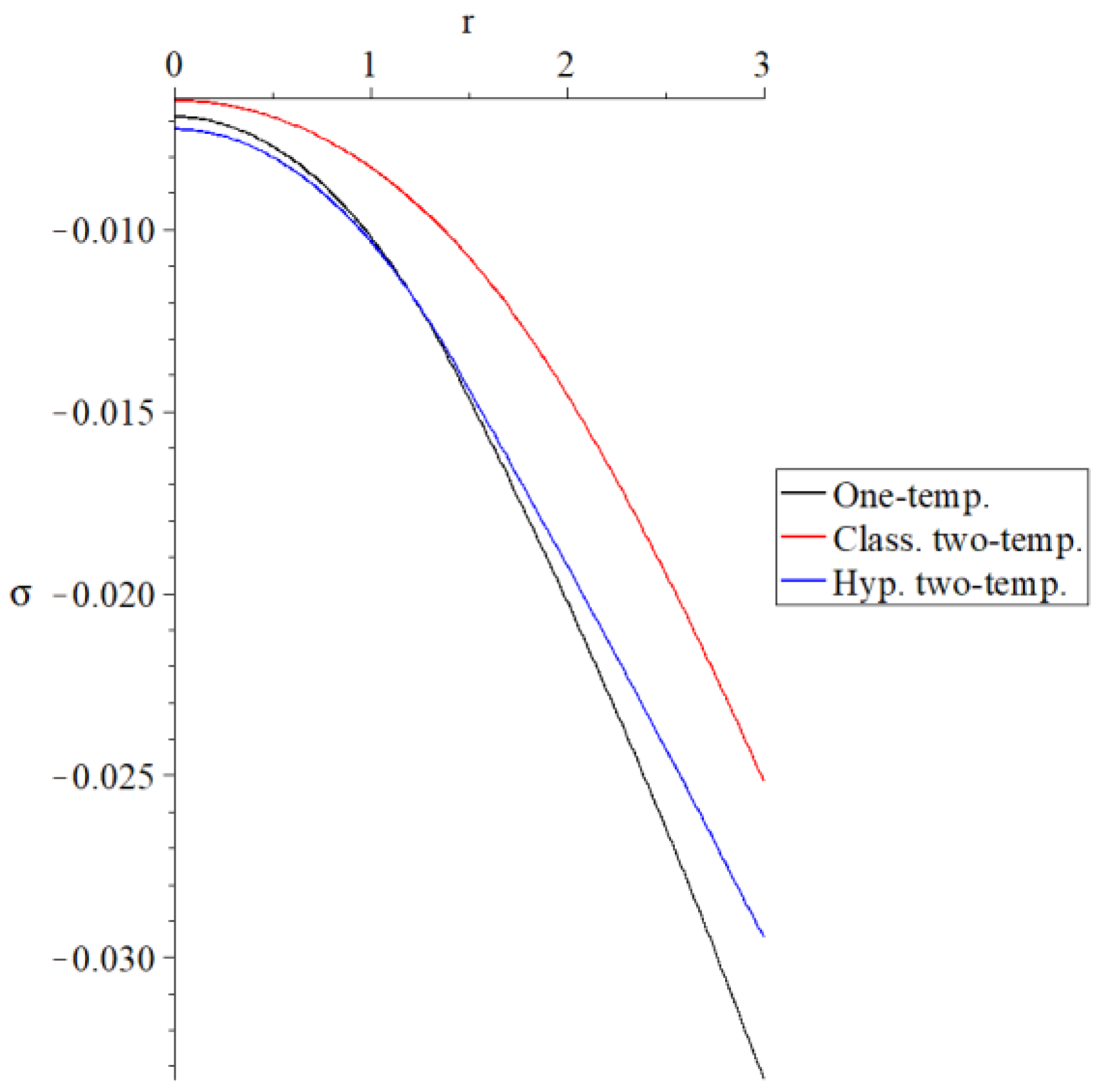
Figure 2, Figure 3, Figure 4, Figure 5 and Figure 6 have been created for various values of the two-temperature parameter ${\delta }^2=\left(0.0,3{\tilde{c}}^2,\frac{3{\tilde{c}}^2}{s^2}\right)$ and the mechanical damage parameter $D=0.2$. The value ${\delta }^2=0.0$ is devoted to the usual L-S model of thermoelasticity with one-temperature; the value ${\delta }^2=3{\tilde{c}}^2$ represents the classical two-temperature model, while ${\delta }^2=\frac{3{\tilde{c}}^2}{s^2}$ represents the hyperbolic two-temperature thermoelasticity model.

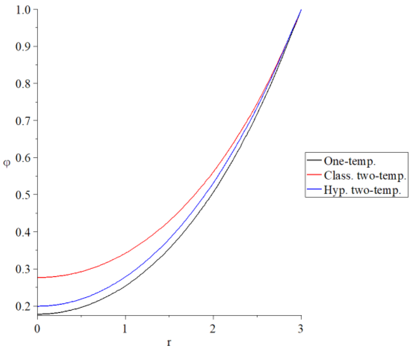
Figure 2 shows the conductive temperature increment distribution in which all of the curves start from the position $r=3.0$ when $\phi =1.0$, which agrees with the thermal shock value as in the thermal boundary condition. The three curves have identical behavior with different values, where the conductive temperature increment distributions have the following order:

$$\phi \left(\mathrm{One}-\mathrm{temp}.\right)<\phi \left(\mathrm{Hyp}. \mathrm{two}-\mathrm{temp}.\right)<\phi \left(\mathrm{Class}. \mathrm{two}-\mathrm{temp}.\right)$$

(69)

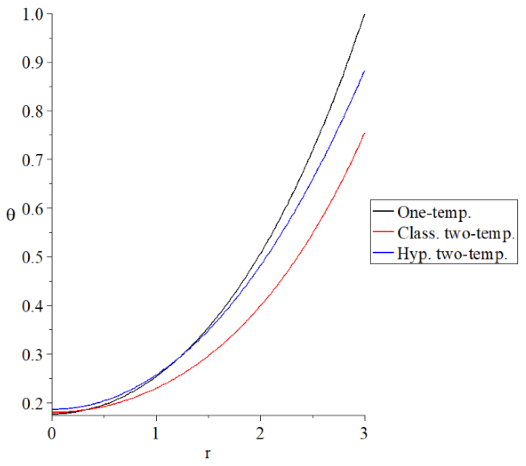
Figure 3 represents the dynamic temperature increment distributions, where the first curve ${\delta }^2=0.0$ represents the one-temperature model, which starts from the position $r=3.0$ with the value $\theta =1.0$. This value agrees with the thermal boundary condition, and the dynamic temperature increment has the following order:

$$\theta \left(\mathrm{Class}.\mathrm{two}-\mathrm{temp}.\right)<\theta \left(\mathrm{Hyp}. \mathrm{two}-\mathrm{temp}.\right)<\theta \left(\mathrm{One}-\mathrm{temp}.\right)$$

(70)

Figure 4 represents the volumetric strain distributions in which all of the curves start from the position $r=3.0$ with zero values, which agrees with the mechanical boundary condition. The three curves have identical behavior with different values. Each curve has a different peak point and takes the following order:

$$\left|e_{\max }\left(\mathrm{Class}. \mathrm{two}-\mathrm{temp}.\right)\right|<\left|e_{\max }\left(\mathrm{Hyp}. \mathrm{two}-\mathrm{temp}.\right)\right|<\left|e_{\max }\left(\mathrm{One}-\mathrm{temp}.\right)\right|$$

(71)

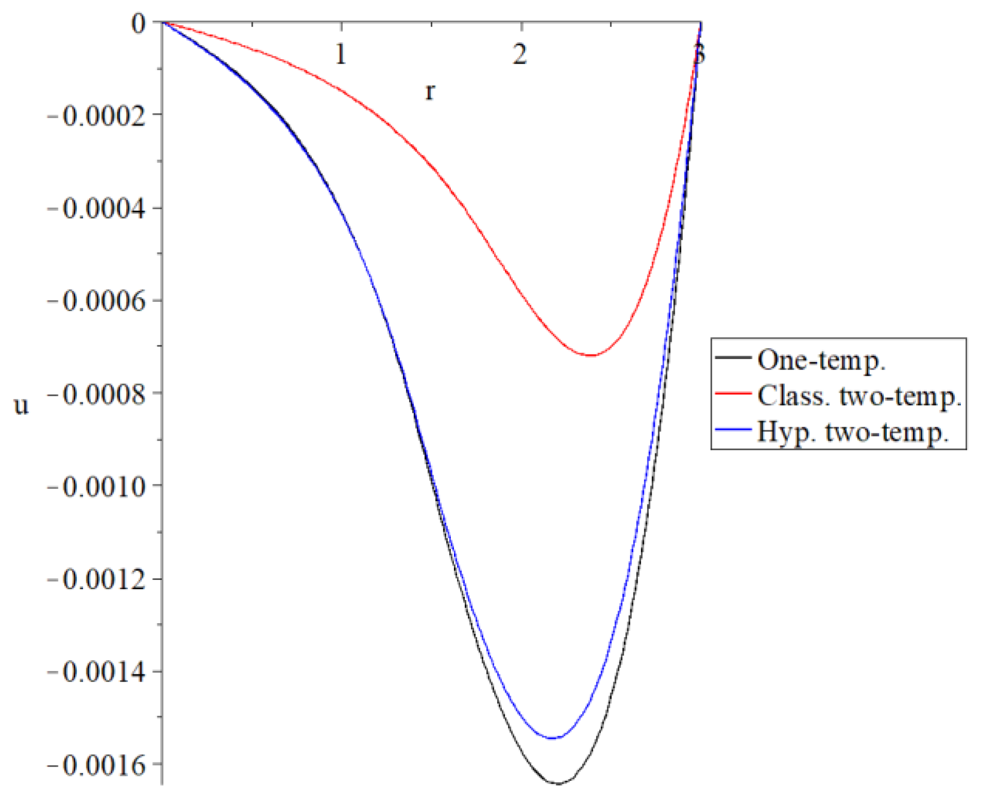
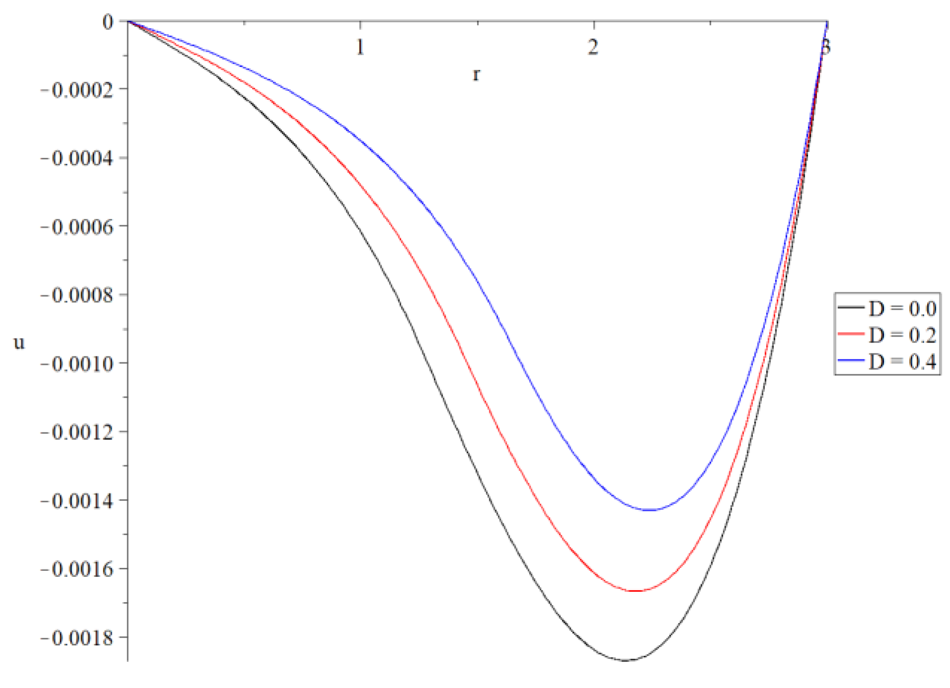
Figure 5 represents the displacement component distributions in which all of the curves begin from the position $r=3.0$ from the zero value. All of the curves have identical behavior with different values, and each curve has a peak point that takes the following order:

$$\left|u_{\max }\left(\mathrm{Class}. \mathrm{two}-\mathrm{temp}.\right)\right|<\left|u_{\max }\left(\mathrm{Hyp}. \mathrm{two}-\mathrm{temp}.\right)\right|<\left|u_{\max }\left(\mathrm{One}-\mathrm{temp}.\right)\right|$$

(72)

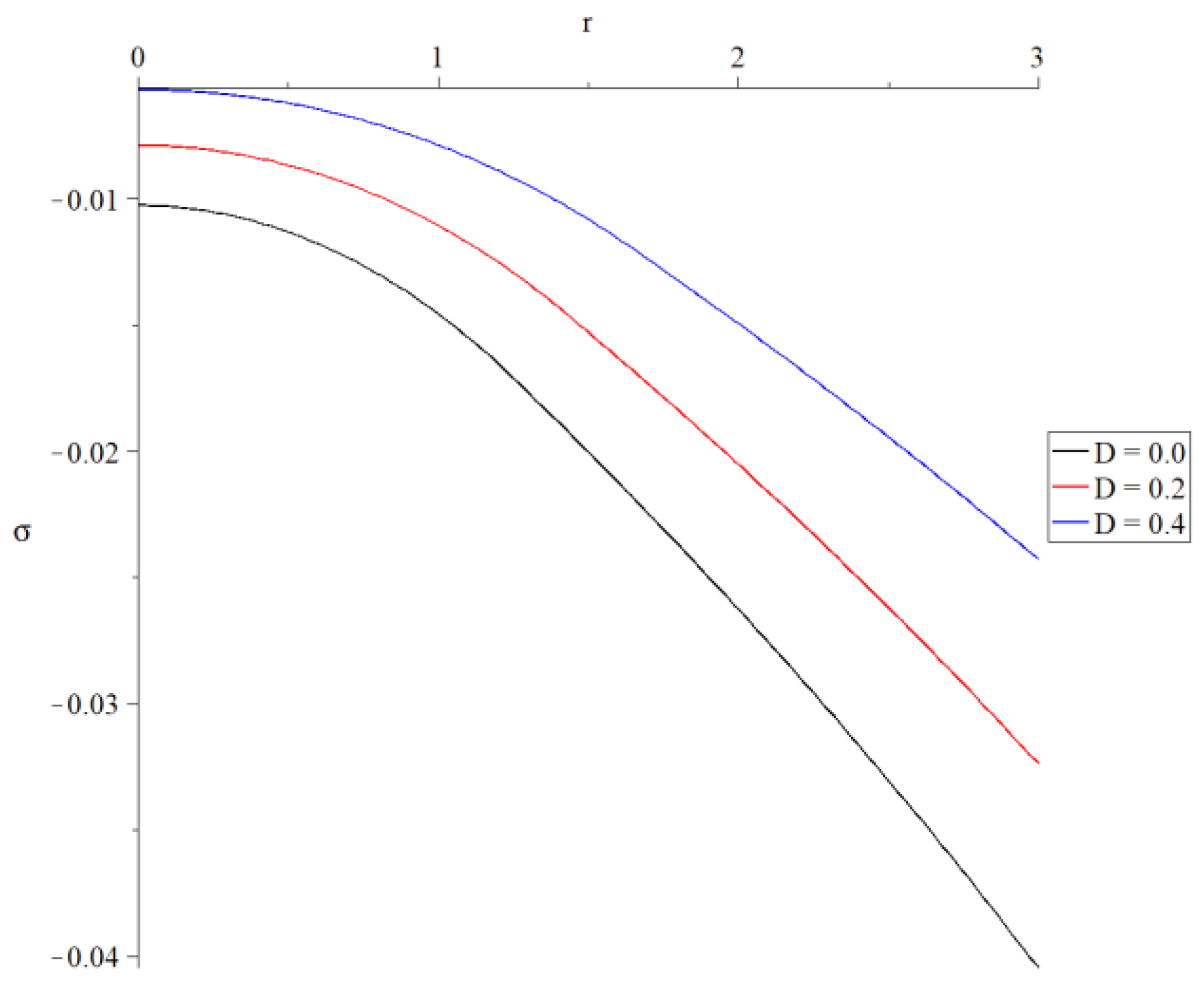
Figure 6 shows the distributions of the average stress, where all the curves begin from the position $r=3.0$ with different values. The three curves have identical behavior with different values. The values of the start points have the following order:

$$\left|{\sigma }_{r=3.0}\left(\mathrm{Class}. \mathrm{two}-\mathrm{temp}.\right)\right|<\left|{\sigma }_{r=3.0}\left(\mathrm{Hyp}. \mathrm{two}-\mathrm{temp}.\right)\right|<\left|{\sigma }_{r=3.0}\left(\mathrm{One}-\mathrm{temp}.\right)\right|$$

(73)

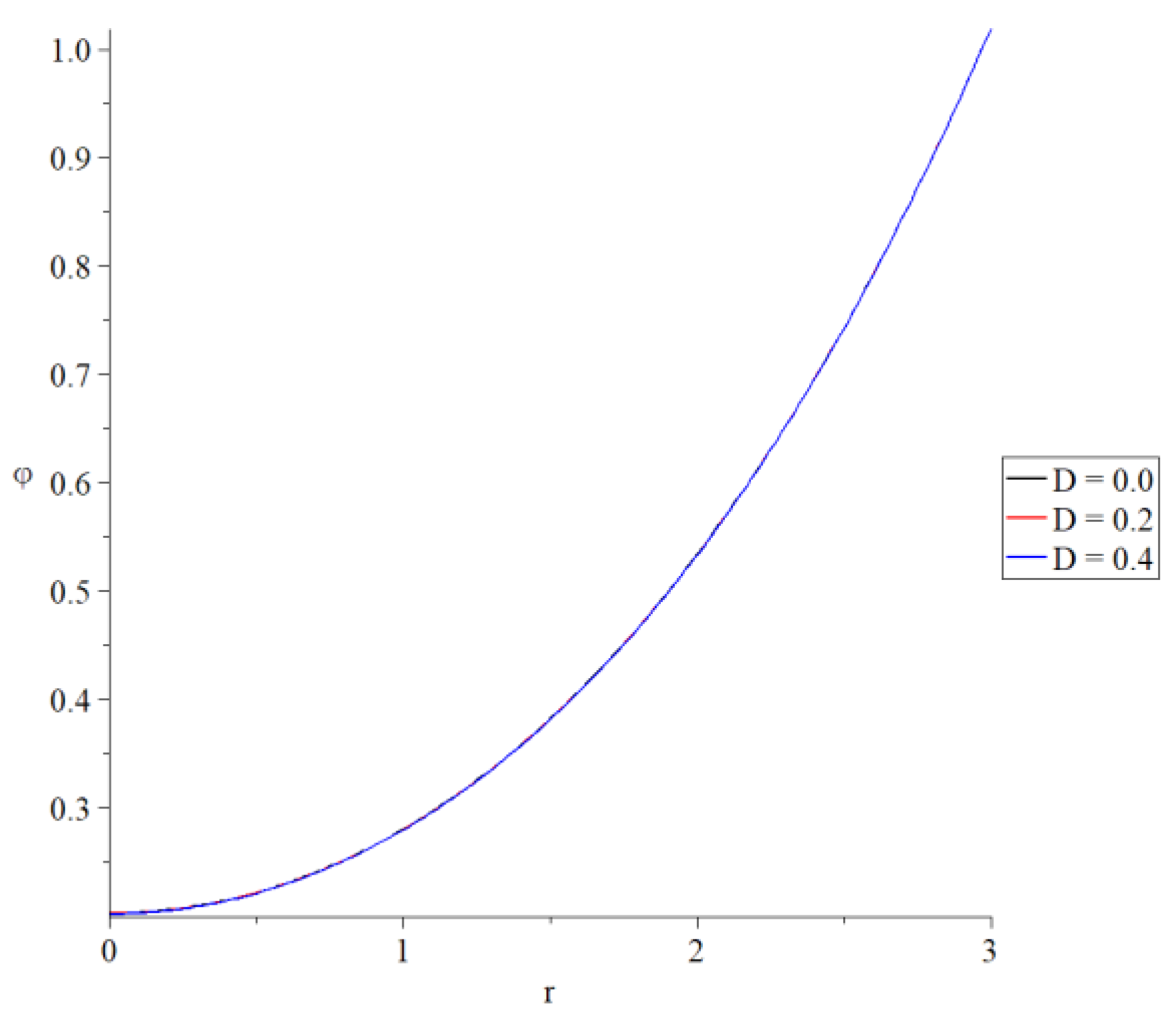
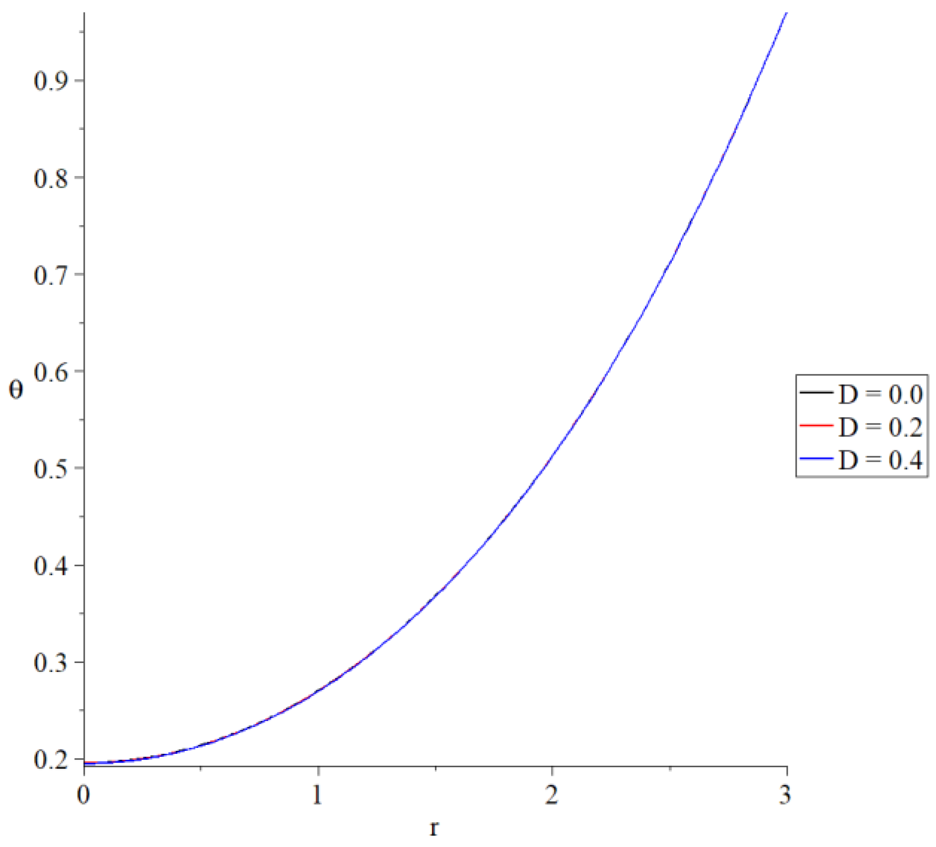
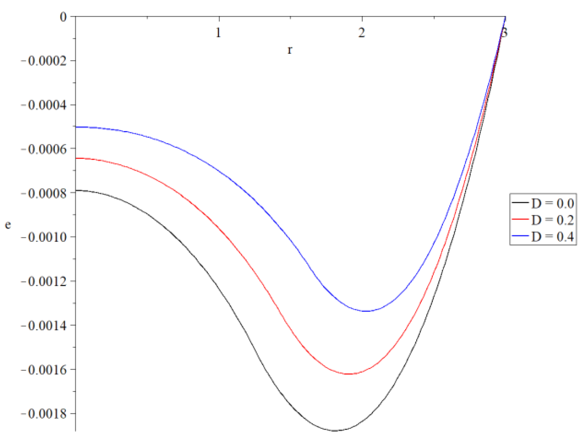
Figure 7, Figure 8, Figure 9, Figure 10 and Figure 11 have been prepared for different values of the damage mechanics parameter when $D=\left(0.0,0.2,0.4\right)$ under the hyperbolic two-temperature thermoelasticity model. The value $D=0.0$ represents the undamaged case, while the values $D=0.2 \mathrm{and} 0.4$ represent two different damage cases.

Figure 7 and Figure 8 represent how the mechanical damage parameter has no effect on the conductive and dynamic temperature increment.

Figure 9 shows that the volumetric strain distribution has a substantial impact on the mechanical damage variable. A rise in the mechanical damage value allows the absolute value of the volumetric strain to decrease. Figure 10 indicates a significant influence on the displacement distribution of the mechanical damage component—a rise in the mechanical damage variable results in a reduction in the absolute displacement value.

Figure 11 indicates a significant influence on the average stress distribution of the mechanical damage variable. A rise in the value of the mechanical damage parameter leads to a decrease in average stress absolute value.

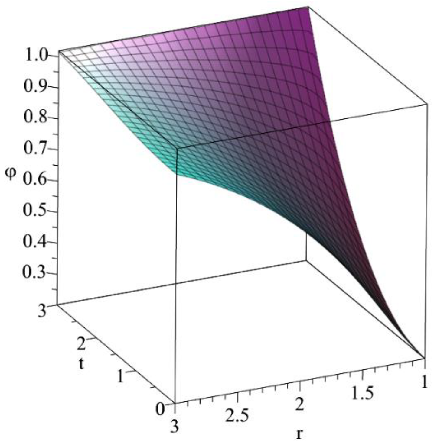
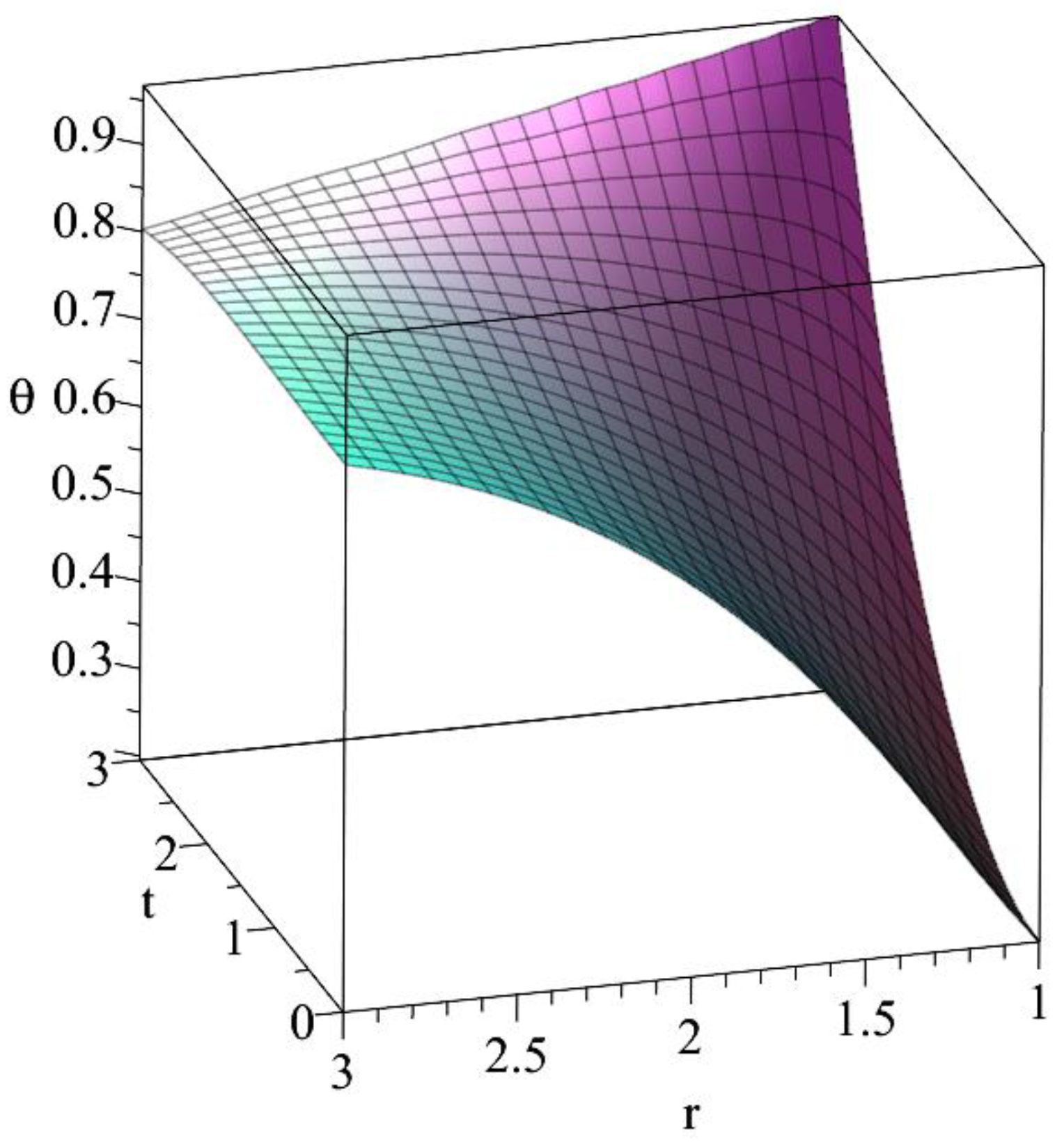
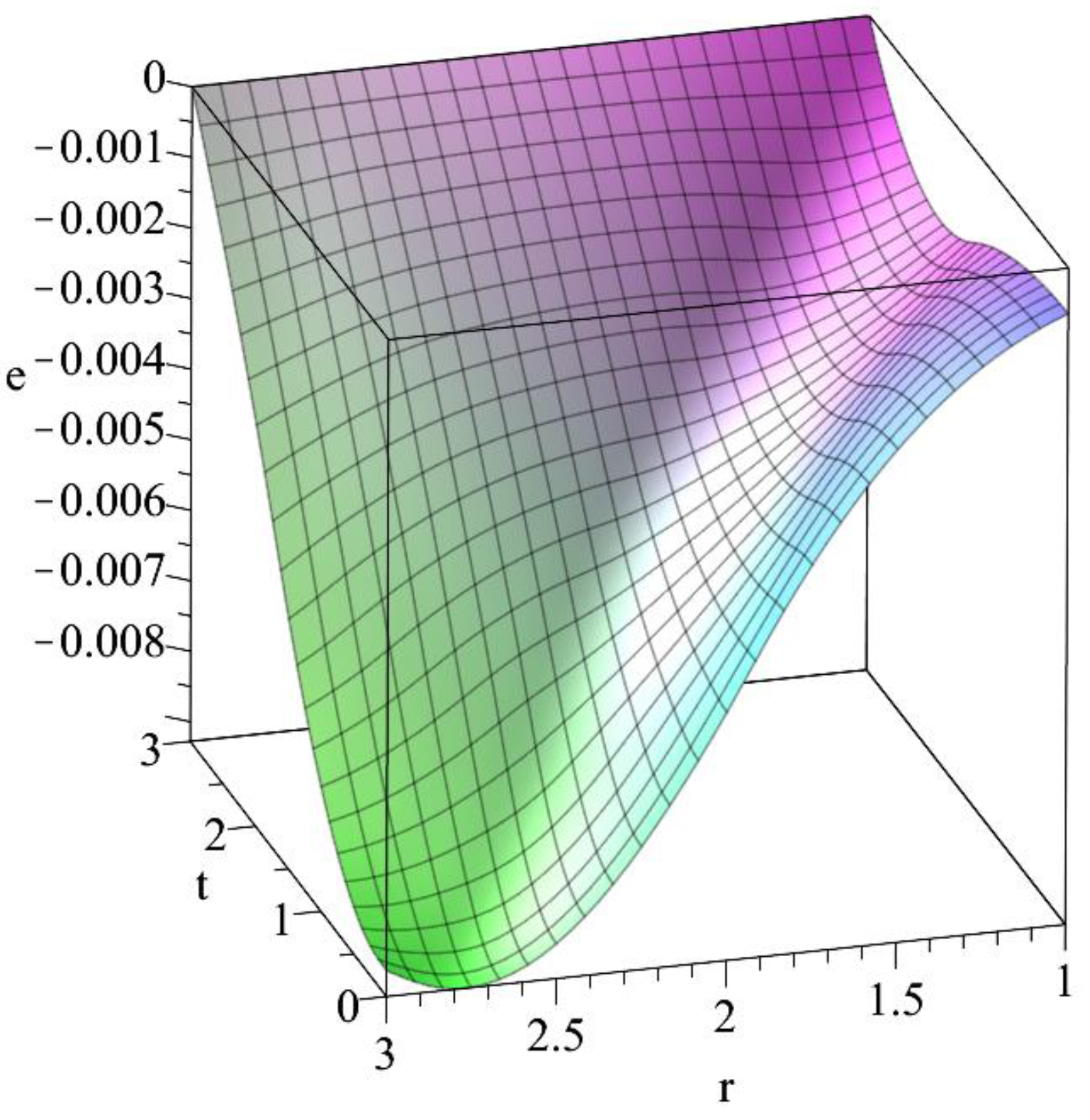
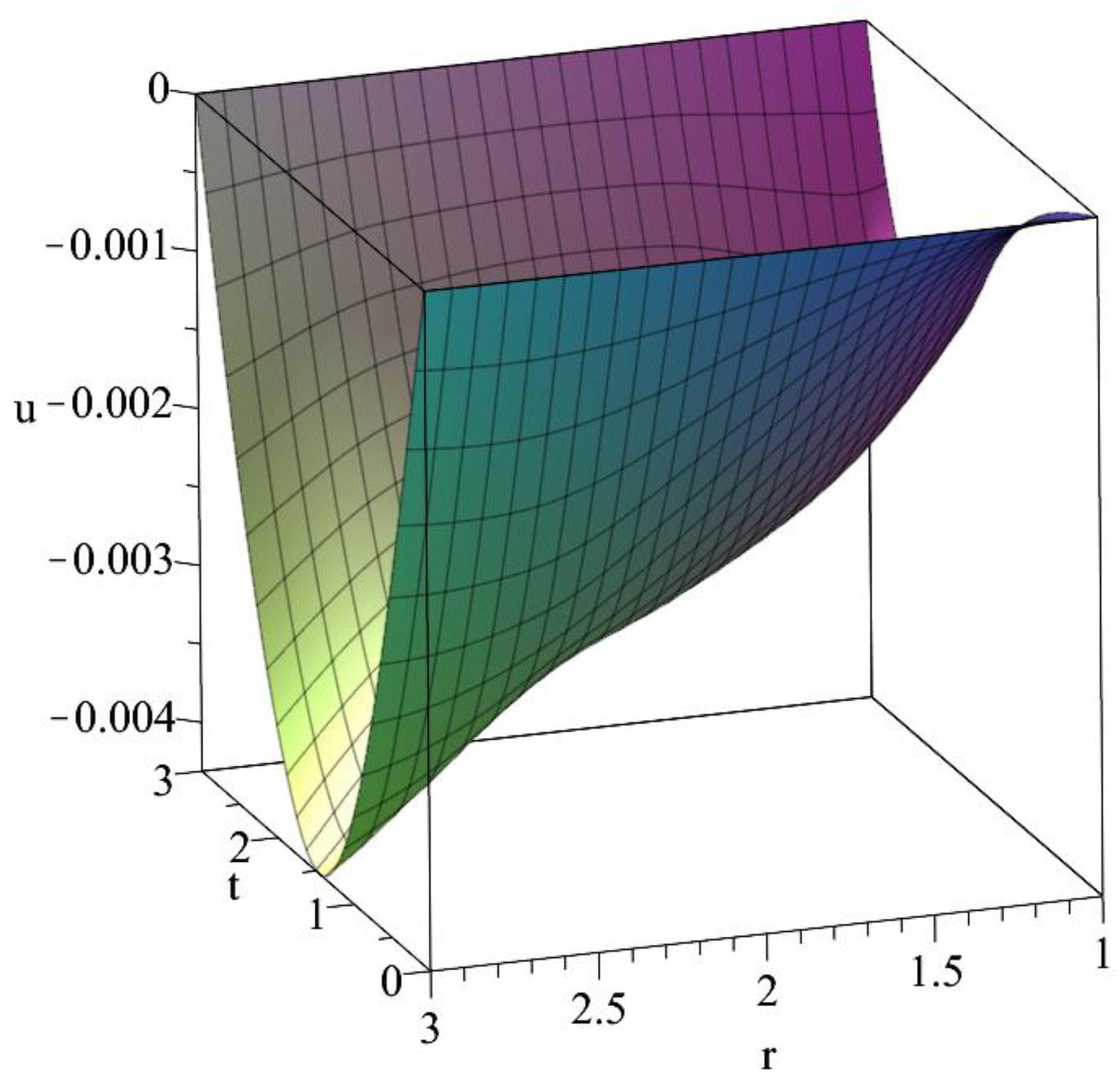
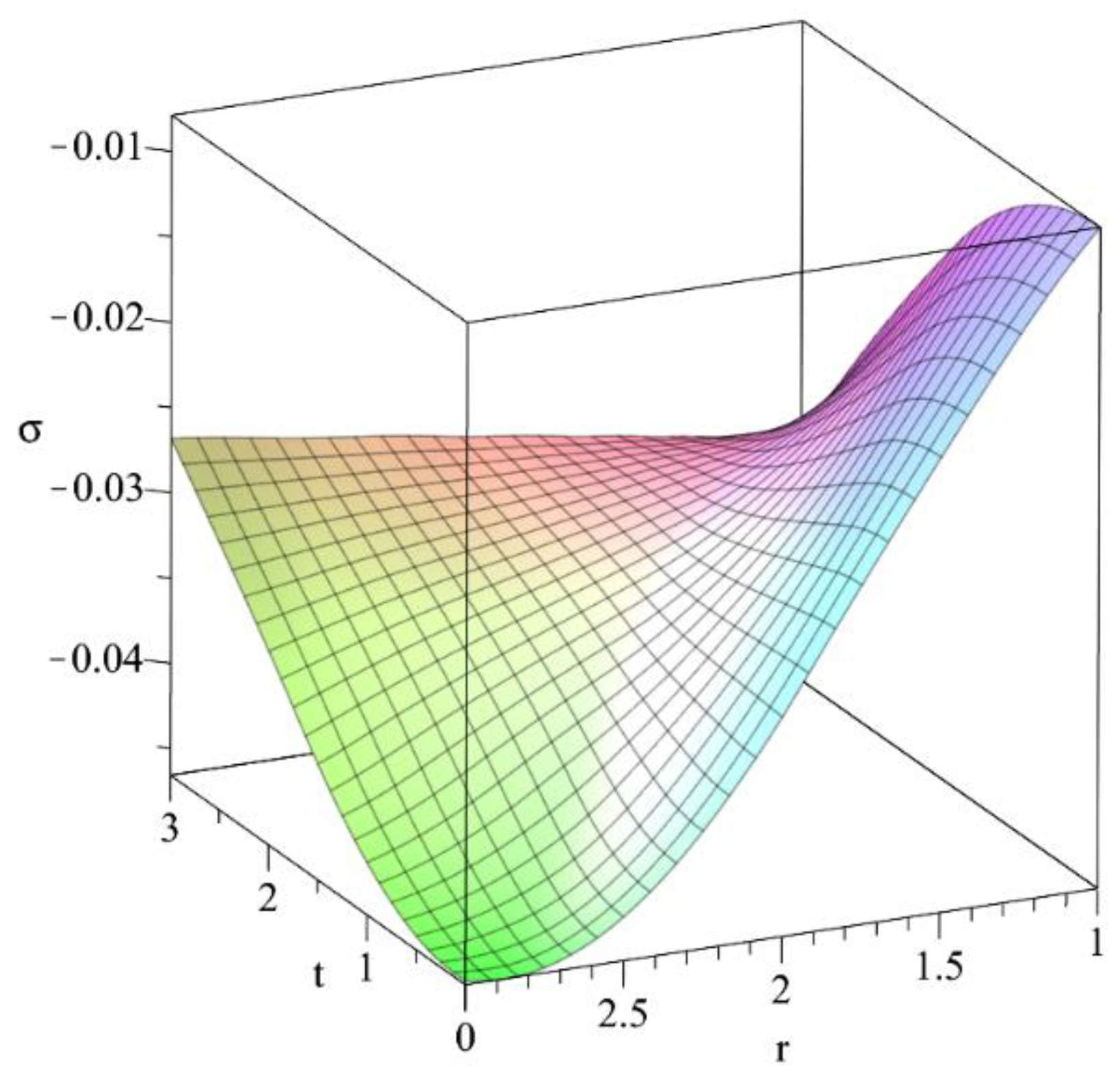
Figure 12, Figure 13, Figure 14, Figure 15 and Figure 16 represent the distributions of conductive temperature increment, dynamic temperature increment, volumetric strain, displacement, and average stress under the hyperbolic two-temperature thermoelasticity model in three dimensions. The figures have been created for a wide range of dimensionless radi $0.0\le r\le 3.0$ and dimensionless time intervals $1.0\le t\le 3.0$. We can see that the value of time has significant effects on all the studied functions. The mechanical and thermal waves propagate with finite or limited speeds under the hyperbolic two-temperature thermoelasticity model, and increasing the time value helps the thermomechanical waves disappear faster.

6. Conclusions

The diagonalization method is used for the first time in this study to create a new model of a homogeneous, thermoelastic, and isotropic solid sphere subjected to mechanical damage. The fundamental equations were derived using the hyperbolic two-temperature generalized thermoelasticity theory while considering mechanical damage.

The one-temperature and hyperbolic two-temperature thermoelasticity models generate thermomechanical waves with finite or limited propagation velocity, according to the computational results.

As a result, the hyperbolic two-temperature thermoelasticity model works well in the characterization of the thermodynamic behaviors of thermoelastic materials.

Furthermore, the two-temperature parameter and time have substantial effects on all of the functions tested, whereas the mechanical damage variable only has a substantial impact on the strain, displacement, and stress distributions.

The conductive and dynamical temperature distributions are unaffected by the mechanical damage variable.

The value of the conductive temperature increment based on the one-temperature model is greater than its value based on hyperbolic two-temperature model and its value based on the classical two-temperature model. The value of the dynamical temperature increment based on the classical two-temperature model is greater than its value based on the hyperbolic two-temperature model and its value based on the one-temperature model.

The absolute values of the peak points of the strain and displacement distributions based on the classical two-temperature model is greater than its values based on the hyperbolic two-temperature model and its value based on the one-temperature model.

References

- Chen, P.J.; Gurtin, M.E. On a theory of heat conduction involving two temperatures. Z. Angew. Math. Und Phys. ZAMP 1968, 19, 614–627. [Google Scholar] [CrossRef]
- Warren, W.; Chen, P. Wave propagation in the two temperature theory of thermoelasticity. Acta Mech. 1973, 16, 21–33. [Google Scholar] [CrossRef]
- Youssef, H. Theory of two-temperature-generalized thermoelasticity. IMA J. Appl. Math. 2006, 71, 383–390. [Google Scholar] [CrossRef]
- Abbas, I.A.; Youssef, H.M. Two-temperature generalized thermoelasticity under ramp-type heating by finite element method. Meccanica 2013, 48, 331–339. [Google Scholar] [CrossRef]
- Youssef, H. Two-temperature generalized thermoelastic infinite medium with cylindrical cavity subjected to different types of thermal loading. WSEAS Trans. Heat Mass Transf. 2006, 1, 769. [Google Scholar]
- Youssef, H. A two-temperature generalized thermoelastic medium subjected to a moving heat source and ramp-type heating: A state-space approach. J. Mech. Mater. Struct. 2010, 4, 1637–1649. [Google Scholar] [CrossRef]
- Youssef, H.M.; El-Bary, A.A. Theory of hyperbolic two-temperature generalized thermoelasticity. Mater. Phys. Mech. 2018, 40, 158–171. [Google Scholar]
- Youssef, H.M.; El-Bary, A.A.; Al-Lehaibi, E.A. Thermal-stress analysis of a damaged solid sphere using hyperbolic two-temperature generalized thermoelasticity theory. Sci. Rep. 2021, 11, 1–19. [Google Scholar] [CrossRef]
- Youssef, H.M.; El-Bary, A.A.; Al-Lehaibi, E.A. The fractional strain influence on a solid sphere under hyperbolic two-temperature generalized thermoelasticity theory by using diagonalization method. Math. Probl. Eng. 2021, 2021, 12. [Google Scholar] [CrossRef]
- Hobiny, A. Effect of the hyperbolic two-temperature model without energy dissipation on Photo-thermal interaction in a semi-conducting medium. Results Phys. 2020, 18, 103167. [Google Scholar] [CrossRef]
- Alshehri, H.M.; Lotfy, K. Memory-Dependent-Derivatives (MDD) for magneto-thermal-plasma semiconductor medium induced by laser pulses with hyperbolic two temperature theory. Alex. Eng. J. 2021. [Google Scholar] [CrossRef]
- Abbas, I.; Saeed, T.; Alhothuali, M. Hyperbolic two-temperature photo-thermal interaction in a semiconductor medium with a cylindrical cavity. Silicon 2021, 13, 1871–1878. [Google Scholar] [CrossRef]
- Youssef, H.M. Generalized thermoelastic infinite medium with spherical cavity subjected to moving heat source. Comput. Math. Modeling 2010, 21, 212–225. [Google Scholar] [CrossRef]
- Youssef, H.M.; El-Bary, A.A. Characterization of the photothermal interaction of a semiconducting solid sphere due to the fractional deformation, relaxation time, and various reference temperature under LS Theory. Silicon 2020, 13, 2103–2114. [Google Scholar] [CrossRef]
- Youssef, H.M.; El-Bary, A. Characterization of the photothermal interaction of a semiconducting solid sphere due to the mechanical damage and rotation under Green-Naghdi theories. Mech. Adv. Mater. Struct. 2020. [Google Scholar] [CrossRef]
- Gross, D.; Seelig, T. Fracture Mechanics: With an Introduction to Micromechanics; Springer: Berlin/Heidelberg, Germany, 2017. [Google Scholar]
- Öchsner, A. Continuum Damage Mechanics, Continuum Damage and Fracture Mechanics; Springer: Berlin/Heidelberg, Germany, 2016; pp. 65–84. [Google Scholar]
- Voyiadjis, G.Z. Handbook of Damage Mechanics: Nano to Macro Scale for Materials and Structures; Springer: Berlin/Heidelberg, Germany, 2015. [Google Scholar]
- Yao, Y.; He, X.; Keer, L.M.; Fine, M.E. A continuum damage mechanics-based unified creep and plasticity model for solder materials. Acta Mater. 2015, 83, 160–168. [Google Scholar] [CrossRef]
- Voyiadjis, G.Z.; Kattan, P.I. Introducing damage mechanics templates for the systematic and consistent formulation of holistic material damage models. Acta Mech. 2017, 228, 951–990. [Google Scholar] [CrossRef]
- Khatir, A.; Tehami, M.; Khatir, S.; Wahab, M.A. Multiple damage detection and localization in beam-like and complex structures using co-ordinate modal assurance criterion combined with firefly and genetic algorithms. J. Vibroeng. 2016, 18, 5063–5073. [Google Scholar]
- Youssef, H.M. Two-temperature generalized thermoelastic infinite medium with cylindrical cavity subjected to moving heat source. Arch. Appl. Mech. 2010, 80, 1213–1224. [Google Scholar] [CrossRef]
- Thibault, J.; Bergeron, S.; Bonin, H.W. On finite-difference solutions of the heat equation in spherical coordinates. Numer. Heat Transf. Part A Appl. 1987, 12, 457–474. [Google Scholar]
- Zill, D.; Wright, W.S.; Cullen, M.R. Advanced Engineering Mathematics; Jones & Bartlett Learning: Burlington, MA, USA, 2011. [Google Scholar]
- Tzou, D.Y. A unified field approach for heat conduction from macro-to micro-scales. J. Heat Transf. 1995, 117, 8–16. [Google Scholar] [CrossRef]
Figure 1.
The isotropic homogeneous thermoelastic solid sphere.
Figure 2.
The distribution of the conductive temperature increment for the variance values of the two-temperature parameter when .
Figure 3.
The distribution of the dynamic temperature increment for the variance values of the two-temperature parameter when .
Figure 4.
The distribution of the volumetric strain for the variance values of the two-temperature parameter when .
Figure 5.
The distribution of the displacement for the variance values of the two-temperature parameter when .
Figure 6.
The distribution of the average stress for the variance values of the two-temperature parameter when .
Figure 7.
The distribution of the conductive temperature increment for the variance values of damage mechanics in the context of the hyperbolic two-temperature model.
Figure 8.
The distribution the dynamic temperature increment for the variance values of damage mechanics in the context of the hyperbolic two-temperature model.
Figure 9.
The distribution of the volumetric strain increment for the variance values of damage mechanics in the context of the hyperbolic two-temperature model.
Figure 10.
The distribution of the displacement for the variance values of mechanical damage parameter in the context of the hyperbolic two-temperature model.
Figure 11.
The distribution of the average stress for the variance values of the mechanical damage parameter in the context of the hyperbolic two-temperature model.
Figure 12.
The distribution of the conductive temperature increment in the context of the hyperbolic two-temperature model when .
Figure 13.
The distribution of the dynamic temperature increment in the context of the hyperbolic two-temperature model when .
Figure 14.
The distribution of the volumetric strain in the context of the hyperbolic two-temperature model when .
Figure 15.
The distribution of the displacement in the context of the hyperbolic two-temperature model when .
Figure 16.
The distribution of the average stress in the context of the hyperbolic two-temperature model when .
Publisher’s Note: MDPI stays neutral with regard to jurisdictional claims in published maps and institutional affiliations. |
© 2021 by the author. Licensee MDPI, Basel, Switzerland. This article is an open access article distributed under the terms and conditions of the Creative Commons Attribution (CC BY) license (https://creativecommons.org/licenses/by/4.0/).
Share and Cite
MDPI and ACS Style
Al-Lehaibi, E.A.N. Diagonalization Method to Hyperbolic Two-Temperature Generalized Thermoelastic Solid Sphere under Mechanical Damage Effect. Crystals 2021, 11, 1014. https://doi.org/10.3390/cryst11091014
AMA Style
Al-Lehaibi EAN. Diagonalization Method to Hyperbolic Two-Temperature Generalized Thermoelastic Solid Sphere under Mechanical Damage Effect. Crystals. 2021; 11(9):1014. https://doi.org/10.3390/cryst11091014
Chicago/Turabian StyleAl-Lehaibi, Eman A. N. 2021. "Diagonalization Method to Hyperbolic Two-Temperature Generalized Thermoelastic Solid Sphere under Mechanical Damage Effect" Crystals 11, no. 9: 1014. https://doi.org/10.3390/cryst11091014
Note that from the first issue of 2016, this journal uses article numbers instead of page numbers. See further details here.