
Application of Fixed-Wing UAV-Based Photogrammetry Data for Snow Depth Mapping in Alpine Conditions


1
Department of Geography and Geology, Faculty of Natural Sciences, Matej Bel University, Tajovskeho 40, 974 09 Banska Bystrica, Slovakia
2
Avalanche Prevention Center, Mountain Rescue Service of Slovakia, 033 01 Liptovsky Hradok, Slovakia
*
Author to whom correspondence should be addressed.
Drones 2021, 5(4), 114; https://doi.org/10.3390/drones5040114
Submission received: 24 August 2021
/
Revised: 29 September 2021
/
Accepted: 6 October 2021
/
Published: 11 October 2021
(This article belongs to the Special Issue Advances in Civil Applications of Unmanned Aircraft Systems)
Abstract
:UAV-based photogrammetry has many applications today. Measuring of snow depth using Structure-from-Motion (SfM) techniques is one of them. Determining the depth of snow is very important for a wide range of scientific research activities. In the alpine environment, this information is crucial, especially in the sphere of risk management (snow avalanches). The main aim of this study is to test the applicability of fixed-wing UAV with RTK technology in real alpine conditions to determine snow depth. The territory in West Tatras as a part of Tatra Mountains (Western Carpathians) in the northern part of Slovakia was analyzed. The study area covers more than 1.2 km2 with an elevation of almost 900 m and it is characterized by frequent occurrence of snow avalanches. It was found that the use of different filtering modes (at the level point cloud generation) had no distinct (statistically significant) effect on the result. On the other hand, the significant influence of vegetation characteristics was confirmed. Determination of snow depth based on seasonal digital surface model subtraction can be affected by the process of vegetation compression. The results also point on the importance of RTK methods when mapping areas where it is not possible to place ground control points.
1. Introduction
Seasonal snow depth distribution represents a key piece of information for many applications, e.g., in hydrology, ecology, or in risk management [1,2,3] with significant environmental and economic impacts [4,5,6,7,8]. Snow depth (symbol from the international classification: HS) denotes the total height of the snowpack, i.e., the vertical distance in centimeters from base to the snow surface [9]. Knowing the best way of snow depth mapping is crucial especially in mountain areas with risk of snow avalanches. In general, there are methods based on sparse in situ measurements with various probes or geophysics measurement techniques [10,11] and methods based on remote sensing. Remote sensing methods represent unmanned aircraft vehicles (UAV) mapping [12,13], conventional airborne mapping and airborne laser-scanning [14,15,16], terrestrial laser-scanning [17,18,19], or usage of satellite imagery [20,21,22]. Especially laser scanning techniques, also known as LiDAR (Light Detection and Ranging), have seen a dramatic widening of applications in the natural sciences [23]. Each of these methods has advantages and self-limits. In the context of snow avalanches, fast deployment and remote sensing are often a key requirement for snow depth mapping. Many mountain areas with avalanche risk are dangerous and difficult to reach in the winter period. These conditions markedly eliminate usage of in situ measurements and therefore, remote sensing is very useful. However, conventional flight missions are often expensive, and their realization is time-consuming with a longer arrangement. Clouds or question of being up to date can be a problem when using very high-resolution satellite imagery. On the other hand, usage of unmanned aerial vehicles or, generally speaking, unmanned aerial systems (UASs) is relatively cost-effective and can be applied very flexibly to cover terrain not accessible from the ground [12,24]. Technological advances and improvements of recent years, including the miniaturization of sensors, as well as autonomous navigation, have significantly lowered the barriers associated with UASs operation [25]. Apart from practical benefits of cost and safety, UASs provide spatial resolution at centimeter scales and can view the surface under cloud cover. Furthermore, UASs can be equipped with a range of possible lightweight sensors (photogrammetric RGB cameras, multispectral, hyperspectral, thermal, LiDAR sensors, atmospheric and gravimetric sensors) according to user requirements or research focus [26]. Nowadays, the usage of UASs for survey purposes such as mapping, 3D modeling, point cloud extraction, and orthophoto generation has become a standard operation [27].
In many studies (e.g., [12,28,29,30]), multirotor platforms of UAVs are used for snow depth mapping despite their relatively short battery endurance and reduced spatial coverage. Longer flight times and bigger area of coverage are the major advantages of fixed-wing UAVs. However, larger fixed-wing drones (e.g., Sirius Pro from MAVinci, UX5 from Trimble or Q-200 from Quest UAS) include quite bulky overall equipment. Flying and necessary arrangements (transport, start preparation, etc.) can be difficult in an alpine environment [12]. Development of fixed-wing UAVs brings improvements in this as well. Drones have dimensions that are more compact. Bodies are demountable, a launch pad is not needed, and all equipment is packable for relatively easy transport (e.g., SenseFly eBee models from Parrot Group or UX11 from Delair). Therefore, the potential usage of fixed-wing UAVs in alpine areas has significantly increased.
The mentioned technologies complemented with progressive image processing techniques and software developments brought new possibilities to 3D (three-dimensional) mapping of the Earth’s surface [25]. Very important is a recent development in photogrammetry which allows high-resolution photorealistic terrain models to be easily constructed [31,32]. Photos from UAVs provide the data for post-processing algorithms such as Structure-from-Motion (SfM) photogrammetry and Multi-View Stereo (MVS) to derive very detailed point clouds of an object or surface. These photogrammetric workflows represent an alternative to LiDAR (e.g., [33,34]). The result of the SfM algorithms is a sparse point cloud with known camera and key point positions [35]. The main advantages of aerial SfM photogrammetry are the speed of measurement in the field, the completeness of the final data, high density of the obtained point cloud, and the low cost of the used UAS. The main disadvantages are higher hardware requirements for image processing and longer office work time [36]. A variety of methods exists to classify points such as bare ground or vegetation in LiDAR point clouds. These filtering techniques may not be directly applicable to photogrammetric point clouds [37]. Because of incorrectly focused images or other factors, there can be some outliers among the points and the resulting dense point cloud can be noisy. Commonly used software packages like Agisoft Metashape (Agisoft LLC) or Pix4Dmapper (Pix4D) include filtering algorithms (depth filtering modes). “Depth filtering” is one of the parameters with the strongest impact on the resulting point cloud. Depth filtering allows outliers from the point cloud, which are caused by poor texture of the scene, noisy or blurry images, to be removed. Depending on the complexity of the scene geometry, different depth filtering modes can be applied. The accuracy of the exported product needs to be analyzed to estimate the complexity of the model and thus select an appropriate depth filtering mode. These are suitable for different conditions or types of surfaces [12]. Application of these filtering techniques in surfaces modeling in diverse conditions of alpine environment (especially snow surfaces) is still a challenge for research.
One of the most essential geospatial outputs of point cloud processing is the Digital Surface Model (DSM). DSM is a digital representation of the horizontal and vertical dimensions related to the Earth including all natural and manmade objects in a grid cell structure [38]. The basic framework for determination of snow depth via UAVs photogrammetry is based on DSM comparison on the principle of differentiating between temporally subsequent surfaces. It means subtracting a snow-free DSM from a DSM with a snow cover [39,40,41]. A snow-free surface (DSM from the snow-free season) provides a reference dataset for absolute snow depth determination. Therefore, the quality of DSM is very important, and it is directly affected by the quality of the point cloud.
The traditional way of UAV-based photogrammetry data georeferencing is dependent on ground control points (GCPs). GCPs are usually measured directly by conventional terrestrial techniques in terrain and are included to UAV data processing. However, this way negates the main UASs advantage of contactless survey. Furthermore, in an alpine environment, it is often dangerous or even impossible. To eliminate this requirement, the data of Global Navigation Satellite Systems (GNSS) with various techniques of corrections are used. Usually, GNSS data are stored within the metadata of the images acquired during flight. Two types of GNSS data corrections are used in UAVs. If the UAV GNSS receiver can communicate with the reference station in real time (using a radio link), corrections can be simultaneously applied during the flight. This mode is referred to as Real-Time Kinematic (RTK) correction. If the corrections from the reference station are applied post-flight, the mode is referred to as Post-Processed Kinematic, or PPK method [42].
The main aim of this study is to test the applicability of fixed-wing UAV with RTK technology in real alpine conditions for snow depth determination. Attention is paid to the quality of DSMs. Several depth filtering modes in UAV data post-processing and their influence on DSMs were evaluated. The influence of several types of surfaces on the accuracy of snow depth determination was also evaluated. The study was carried out in a specific mountain environment with high elevation and varied vegetation cover. We assumed that it is the varied vegetation and its properties that can have a major impact on the resulting data.
2. Materials and Methods
2.1. Study Area
Žiarska valley is located in West Tatras as a part of Tatra Mountains (part of the Western Carpathians) in the northern part of Slovakia. The valley is one of the most avalanche-prone locations in the Carpathian mountain range. The avalanches frequently pass over the road and threaten the visitors and mountain cabins. The area has a rich avalanche history record. In the March of 2009, large catastrophic avalanches were observed from the massif of Príslop. In the morning hours of 25 March 2009, seven large slab avalanches were simultaneously triggered, and snow formed a 2 km long deposit. Two cottages, an automatic weather station, and a concrete bridge were damaged together with 280,000 m2 of the forest. This was one of the most severe avalanche cycles in the Carpathian Mountain range. Fortunately, the road was closed and the cottages were evacuated. Careful monitoring is crucial in case of possible evacuations.
The most critical slopes of Žiarska valley as far as avalanches are concerned have been chosen for analysis. The total area of the analyzed polygon was 121.1 ha. The altitude of study area is between 1210.9 and 2103.9 m (ASL). The slope angle of the study area is from 2.6 to 41.8 degrees. The land cover of the study area is very variable. It is a mixture of alpine grasslands, shrubs (mainly growth of Vaccinium myrtillus or Vaccinium vitis-idaea with height < 1 m) and disperse areas of mugo pine (Pinus mugo with height 1–3 m) containing steep rocky outcrops and rubble fields in higher altitudes. Sparse larchs (Larix decidua), pine trees (Pinus sylvestris), and groups of deciduous vegetation (e.g., Sorbus aucuparia, Acer pseudoplatanus, Betula pendula) are located in lower altitudes, especially in the western and southern parts of the study area. The location of the study area is provided by Figure 1.
2.2. Acquisition of Photogrammetric Data
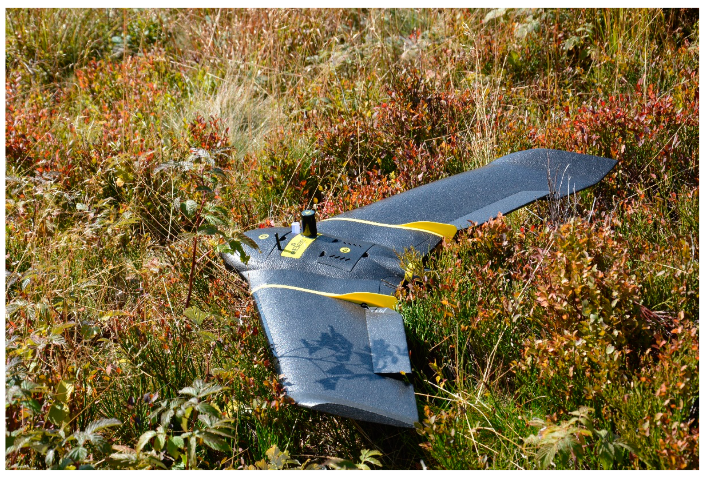
To obtain photogrammetry data, a fixed-wing UAV SenseFly eBee Plus (Parrot Group, Switzerland) with activated GNSS RTK/PPK technology was used (Figure 2). The wingspan of UAV is 110 cm, weight is 1.1 kg, and maximum flight time is declared as 59 min. Wind resistance is up to 45 km/h. As a camera, SenseFly S.O.D.A. was used. The 20 megapixel camera (1 inch sensor size) with global shutter acquires regular image data in the visible spectrum. Focal length is fixed to 10.6 mm (comparable with 29 mm focal length on a 35 mm film camera), aperture is F2.8. The UAV was equipped with a dual-frequency (GPS and GLONASS) GNSS receiver. The manufacturer declares absolute X, Y, Z accuracy down to 3 cm for the RTK method and 5 cm for the PPK method. Flight missions were carried out on 30 August 2018 (summer flight mission) to obtain a snow-free DSM and on 29 March 2019 (winter flight mission) to obtain a snow-covered DSM. During all the missions, the sky was clear or only partially cloudy, with no precipitation. For flight mission planning and control, eMotion 3 software was used. For each flight mission, a set of about 650 photos was obtained. In winter, the flight mission was divided into two continuing parts. The reason was the reduced battery life in low temperatures. The image overlaps were 78% (lateral overlap) and 60% (longitudinal overlap). The assumed resolution (Ground Sampling Distance—GSD) calculated by eMotion 3 software was 3.8 cm/px.
We used the PPK mode, where raw GNSS data were recorded during the flight and subsequently post-processed using the differential correction data from the nearest reference station of the Slovak positioning service—SKPOS (in this case, Liptovský Mikuláš station). SKPOS represents active geodetic control of Slovakia. Physical geodetic points on which antennas of SKPOS receivers are mounted make up the reference stations’ network of global navigation satellite systems, the essential part of which forms the highest class of geodetic control points, i.e., the A class of the National Spatial Network. The network of SKPOS reference stations consists of the reference stations located on the territory of Slovakia, but also of the reference stations located in adjacent foreign countries. PPK was carried out in the eMotion 3 software environment. The service enables users to work on-line through a GSM network (real-time) or in a post-processing way. For a fixed solution, the declared SKPOS accuracy in RTK mode is between 2–4 cm (SKPOS_cm) and from 2 mm to 1 cm in PPK mode (product SKPOS_mm) for very precise geodethic measurements (SKPOS, http://www.skpos.gku.sk, accessed on 8 October 2021).
2.3. Processing of Photogrametric Data and DSM Analysing
Subsequently, the data were processed in Agisoft Metashape Professional 1.6 software (Agisoft LLC) using the standard workflow to generate georeferenced DSMs and orthophotos using dense point cloud generation with the default parameters. Agisoft Metashape software is credited to be among the most reliable [43] and accurate [44,45]. Accuracy of the alignment of the images was set to the value high. The expected accuracy of the resulting point cloud was 1–2 times the GSD [46,47]. Quality of dense cloud generation was set as high quality (second highest level). This setting slightly increases the difference between GSD and DSM resolution. However, it was chosen as a suitable compromise between processing time and the expected output quality. During the processing, four modes of depth filtering (disabled, mild, moderate, and aggressive) were used to reduce outliers. Using four depth filtering modes, four separate DSMs from the summer flight mission and four separate DSMs from the winter flight mission were generated.
The main part of the analysis process was the comparison of seasonal digital surface models to determine the vertical change between them for each pixel. This part of the process was carried out in the ArcGIS software environment. Firstly, the reference DSM from summer flight mission was chosen. All four DSMs from the summer flight mission were analyzed. For this purpose, 24 additional checkpoints (CP) were placed in the study area. For location of checkpoints, Stonex GNSS Rover technology was used.
The Stonex S9III Plus instrument was used as the GNNS receiver, for which the manufacturer states mode the declared accuracy for horizontal measurements in the RTK at 2.5 mm ± 0.1 ppm RMS, and for vertical measurements it is 3.5 mm ± 0.4 ppm RMS in the High Precision Static Surveying variant (long time observations). To increase the accuracy and verify the repeatability of the measured values, the resulting values were an average of 3–5 measurements at each point with a high number of repeated observations (60%). S9III Plus is a multi-constellation GNSS receiver, able to receive three GPS signal frequencies: GLONASS, Compass/Beidou, and ready for GALILEO constellation. The receiver was paired with a Stonex S4H controller (handheld GPS with Carlson SurvCE application) via Bluetooth. The spatial coordinates of the measured CPs were registered and recalculated into the national reference coordinate system S-JTSK [JTSK03] (Bessel ellipsoid 1841–basic meridian Ferro, Krovak projection).
The additional checkpoints were distributed in approximately the entire examined area. CPs were located according to real field accessibility, mostly on solid rock fragments in grass or in a growth of mugo pine. The altitude (Z coordinates) of these additional checkpoints (ZCP) was compared with the altitude of the same locations (the same X and Y coordinates) in all four separate DSMs. Altitudes from DSMs (ZDSM) were obtained by ArcMap 10.5 (Esri) using the Extract Values to Points tool on checkpoint positions. Comparison of altitudes was carried out using Equation (1), where Dalt represents difference in altitude. The influence of using depth filtering modes on the comparison results was statistically evaluated by a one-way ANOVA test. The reference DSM was chosen on the basis of this comparison.
Dalt = ZDSM(1;4) − ZCP,
In the next phase, all four separate DSMs of snow-covered surfaces (DSM(1;4)) were compared with the reference DSM (DSMref) from the summer flight mission. The comparison process was operated in ArcMap 10.5 (Esri) using the Raster calculator tool. Models of snow depth (HSM(1;4)) were derived on the basis of DSMs differences according to Equation (2):
HSM(1;4) = DSM(1;4) − DSMref,
All HSMs as a result of the main comparison process were checked using in situ data of snow depth. These data were obtained manually by a snow probe on the same day as the winter flight mission. Aluminum avalanche probes with 0.01 m graduations were used. Overall, 10 snow probe checkpoints (SPCP) were placed in the terrain. SPCPs were located on two types of vegetation cover, completely overlaid by snow at that time. The majority of SPCPs were located on an alpine grass cover with small shrubs (e.g., growth of Vaccinium myrtillus or Vaccinium vitis-idaea). The rest of the points were located in areas with a mugo pine cover (growth of Pinus mugo). Due to the high avalanche risk and real accessibility, it was not possible to place a larger number of SPCPs or place SPCPs in a regular distribution. The position of each SPCP was located by a Stonex GNSS Rover using SKPOS (RTK mode). Finally, the in situ data from the position of all SPCPs were compared with the data of HSMs. The influence of using depth filtering modes on the comparison results was statistically evaluated by a one-way ANOVA test. All components of workflow are provided in Figure 3.
3. Results and Discussion
3.1. DSM from the Summer Flight Mission and Selection of Reference DSM
During the summer flight mission, 656 images were obtained, and all of them were successfully aligned by software processing. The alignment of cameras on 100% and RMS reprojection error of about 1 pixel grade gave a presumption of a relatively accurate output (Table 1). According to processing results, the total error of camera location was rounded to 2.49 cm.
The average camera location errors are the only accuracy measure when no ground control points are used. Tomaštík et al. [42] state that this value is unreliable for the estimation of actual accuracy. Error values can be false optimistic. However, according to their study, horizontal errors of the PPK solution did not exceed 10 cm in comparison with that of the GCP method. This can be considered as an acceptable error in this type of alpine environment. Gerke and Przybilla [48] confirm a high level of accuracy of the PPK method. According to their study, addition of GCP to the PPK method did not even bring better accuracy. However, this study was carried out in an area with a maximum height difference of 50 m. The application of GCP and their regular spatial distribution can undoubtedly have a positive effect on accuracy. However, this cannot be mostly ensured for specific mountain conditions, especially in the winter season. Further, the exact identification of GCP on aligned images can also be problematic, especially in conditions of natural areas [49]. The expected increase in accuracy may not arise.
In general, the lower level of DSM resolution compared to the expected GSD was based mainly on the dense cloud generation setting. Differences in DSM resolution and point density values for each depth filtering mode were not very distinct (Table 2). The resolution and point density values were slightly better for the Moderate and Aggressive modes.
The selection of a reference DSM from the summer flight mission was performed by means of altitude differences at 24 checkpoints (CP). Altitude differences on each DSM were statistically evaluated by using a one-way ANOVA test. However, statistical significance was not confirmed (F 0.4699; p-value 0.7040; F crit 2.7036). The test results showed a p-value of more than 0.70. This value suggested a high level of confidence that the null hypothesis gave an adequate model for the data. The F value was way below the critical F value (F crit). It means that the influence of several depth filtering modes on altitude differences did not have statistical significance.
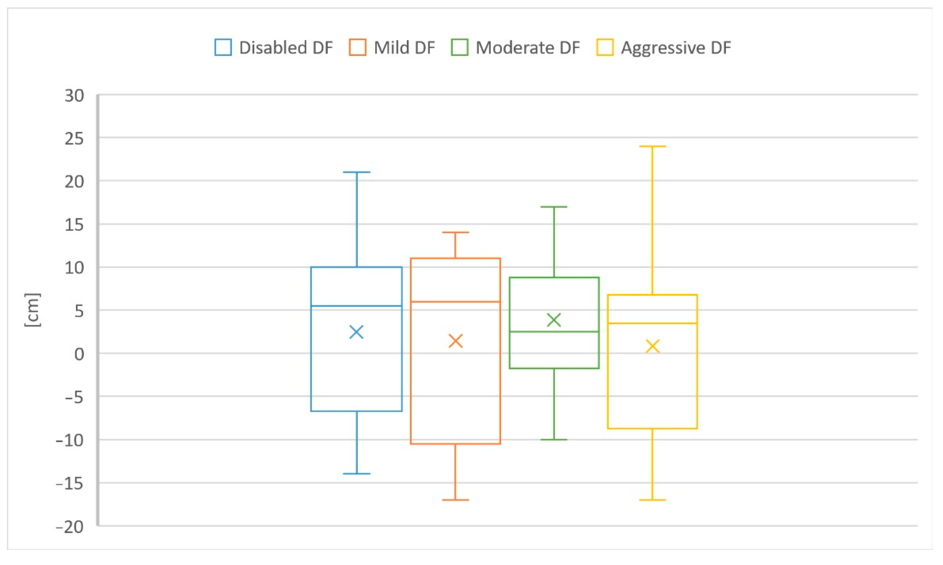
Figure 4 represents total differences of altitudes. The DSM with the Moderate depth filtering (DF) mode had the smallest spread of differences values. Extreme values were 17 cm under the altitude of CP (positive values) or 10 cm above the altitude of CP (negative values) at most. The average value of differences was +3.88 cm, and the median value was −1.75 cm.
The spatial distribution of all CPs is represented in Figure 5. At most CPs there were altitude differences under or above the altitude of CPs at the level up to 5 cm. Positive values prevailed. Bigger altitude differences (positive or negative) were observed especially on the surface of small water streams (Figure 5a) and natural hiking trails (Figure 5b) in central and southern parts of the study area. These were mainly various rock protrusions, which differed slightly in height from their surroundings. Differences can thus be the result of the interpolation process. Positive differences may be caused by a well-known type of error connected with the SfM procedure, including predisposition to vertical arching of the final digital surface [50]. They result from the combination of near-parallel imaging directions and an inaccurate correction of radial lens distortion [51]. Nesbit and Hugenholtz [52] also confirmed the presence of systematic vertical deformations (i.e., “dome effect”) within UAV–SfM datasets. According to their study, the imaging angle has a profound impact on accuracy and precision of data acquisition, with a single camera angle in topographically complex scenes. These potential errors can be prevented by adjusting flight parameters and making oblique images [47,52]. However, when using fixed-wing UAVs, it is often not entirely possible to follow these principles. The discrepancies may be caused by these factors. This needs to be taken into account when evaluating the results. After evaluation of the results mentioned above, the DSM generated by the Moderate depth filtering mode was selected as a reference model.
3.2. DSMs from the Winter Flight Mission
Transport of snow to depressions is a reliable and predictable process. Once a depression is full of snow, a relatively smooth and homogenous surface is created [16,53]. Homogeneous snow surfaces may represent particularly challenging targets for photogrammetry and SfM techniques [25,54]. It is due to its relatively uniform surface and high reflectance relative to snow-free areas, which limit identifiable features [55]. Nevertheless, the imaging quality provided sufficient contrast across snow as well as when the imaging mixed snowy and bare ground conditions. During the winter flight mission, 650 images were obtained, and all of them were successfully aligned. The RMS reprojection error and camera location errors are presented in Table 3. In general, these data are relatively similar to the data from the summer flight mission.
Data on the resolution of DSMs and point density for each depth filtering mode are in Table 4. The best values were obtained using the Moderate depth filtering mode. However, the established differences were very small.
In the winter season, the majority of the study area was covered by a relatively homogeneous snow cover (Figure 6a) or a snow cover with disperse trees and mugo pine patches above the snow surface (Figure 6b). It is known that the photogrammetry process can yield different errors in DSM [49], and it can be assumed that light and a mainly homogenous surface, especially when it is covered by fresh snow, increases these errors [56]. However, the data on resolution and point density of DSMs from the winter flight mission gave a presumption of relatively high precision. In addition, other factors have a more significant effect on the accuracy of snow depth, which is described in the next section.
3.3. Snow Depth Models
The reference DSM was subtracted from the DSM of the snow-covered surface according to Equation (2). Usage of four depth filtering modes brought four DSMs of the snow-covered surface. The results were four snow depth models (HSMs). Each HSM was compared with in situ data of snow depth (SPCP). The results are presented in Table 5. The locations of snow probe checkpoints are represented in Figure 7.
Using various depth filtering modes, it was possible to calculate total average differences between in situ data and HSM data from 82.90 to 86.80 cm (Table 5). The average values might indicate the usage of aggressive depth filtering (HSM4) to be the most appropriate. However, the statistical significance of differences using a one-way ANOVA test was not confirmed (F 0.0039; p-value 0.9997; F crit 2.8663). It means that influence of various depth filtering modes on differences of HSMs was not statistically significant. The obtained results thus confirmed the findings of Boesch et al. [57]. In their study (from Brämabühl in the Swiss Alps) on comparison of snow surface DSM, aggressive filtering of dense point clouds had only little effect in comparison with that of moderate filtering. In general, the aggressive depth filtering mode is recommended if the area to be reconstructed does not contain meaningful small details [58]. Snow-covered surfaces usually correspond to this. Lamsters et al. [56] also confirm this approach in a study from West Antarctica. Outputs of this study were, among other things, the first high-resolution orthophoto maps and digital surface models of the largest Argentine Islands on the basis of UAV photogrammetry.
According to the results in Table 5, the data of snow depth obtained by DSMs comparison method (HSM(1,4) data) were predominantly lower than the real values obtained by snow probes on checkpoints (SPCP data). It is in accordance with the findings of Adams, Bühler, and Fromm [45]. In their study, snow depth values mapped with the UAV were generally lower than snow depth values measured with manual probing. According to Table 5, noticeable differences were observed between the real snow depths and the models, especially in the areas with mugo pine. The obtained data concerning snow depth point to a key influence of vegetation to accuracy. Photogrammetrically derived snow depths may be affected by the compaction of vegetation below the snowpack [25,55]. The summer surface mapped by DSM is created by the top of the vegetative canopy. In the winter, this canopy becomes compressed to the point where it can even produce “negative” snow depths [55], in other words, negative HS. Due to the presence of specific vegetation (especially mugo pine), about 23% of “negative” snow depth areas (snow depth < 0 m) were observed (Figure 7). A resulting snow depth model obtained using the winter DSM with the aggressive depth filtering mode is presented in Figure 7.
Difference fields data (Table 5) can approximately indicate heights of vegetation in the snow-free season on SPCP. However, such extrapolate heights are relatively inaccurate. Data may be affected by several factors. One of them is the fact that the vegetation reaches a certain height (significantly reduced) even under a snowpack.
For a surface with mugo pine, the obtained values are misleading. Snow-covered surface in areas with mugo pine were on average about 170 cm below the surface of reference DSM (Table 5). Locality 1 in Figure 7 illustrates this situation. This part of the study area is covered by extensive growth of mugo pine (1a). However, in the winter season, the area was covered by a relatively plane snow surface (1b). The vegetation was markedly compressed by the weight of the snowpack. The result was an area of negative (<0 m) snow depth (1c). The method of simple comparing seasonal DSMs proves to be inappropriate in this case. As Figure 8a shows, the flexibility of the mugo pine is extreme. According to Redpath, Sirguey, and Cullen [25], the effects of vegetation compression are the greatest in the early winter. Ongoing subsidence of vegetation below the snowpack through midwinter and spring is expected to be minimal. After the snowpack is melted, the mugo pine reaches its original height (Figure 8b). Cavities created by decrease of higher vegetation can also affect the accuracy of in situ probing of snow depth. The range of errors with snow probe measures according to Nolan, Larsen, and Sturm [55] and Harder et al. [40] is about 2 cm and from 5 to 10 cm according to Prokop et al. [59] and Bühler et al. [12]. This fact needs to be taken into consideration when evaluating the differences between HSM data and in situ data. In snow-free season, there are heights of mugo pine growths approximately two meters with local variations. Difference fields data (Table 5) approximately confirmed this height.
On the other hand, the effects of vegetation compression are significantly lower in areas covered with grass and smaller shrubs. The mean difference on this cover type was approximately 24.5 cm (Table 5). The height of vegetation in these areas is from 15 to 45 cm in the summer season. Lower or higher growths may occur locally. It is also a very heterogeneous surface. Among the groups of taller grasses and shrubs, smaller or larger patches of low grass mosses can be found. The deformation of such a land cover under the weight of a snowpack can thus reach a level from a few centimetres to a few decimetres. The similar level of HS difference was also found by Bühler et al. [12]. This study was performed in the Davos region (Switzerland). The study area represented a typical terrain character of alpine environments and natural conditions that partly resembled the conditions in the study area of Žiarska valley. Errors for HS below 30 cm are also described in many studies based on UAV photogrammetric data (e.g., [39,45,60]).
A specific situation was observed in parts of the study area with lower altitudes where deciduous vegetation (e.g., Sorbus aucuparia, Acer pseudoplatanus, Betula pendula, Larix decidua) is located. An example is locality 2 in Figure 7. Due to seasonal changes, the earlier surface of canopies (2a) disappears, and only sparse branches remain (2b). These structures cannot be correctly photogrammetrically modelled in the given resolution. The result was negative snow depths (<0 m) again (2c).
Due to difficult accessibility and real avalanche risk, it was not possible to obtain in situ data from another type of surface (especially a rocky surface with alpine grass patches). This type of surface is located in higher positions with steep slopes. However, based on the findings of Adams, Bühler, and Fromm [45], relatively high reliability of snow depth data from this surface type areas can be assumed. Furthermore, the usage of RTK GNSS technology is generally considered to be more accurate in similar conditions [40,45].
The usage of RTK solutions brings a crucial advantage in inaccessible or hard-to-reach alpine areas. The resulting model accuracy should correspond to that of the RTK GNSS; the standard deviation should, therefore, not exceed several centimeters. Many studies (e.g., [42]) used such an approach, with satisfactory results. On the other hand, studies such as [47,52] point to vertical deviations and errors that can also occur when using RTK technology. Our results are based on a comparison of two models, and each model may be affected by some inaccuracy. The resulting deviation of snow depth model can be a multiple or a reduction of these errors. Unfortunately, this shortage was caused by the variable local properties of the model area. Our study was realized in real alpine conditions on a relatively big area with all natural factors and limits (e.g., fast change of weather, especially wind conditions, and difficult terrain accessibility). One of the aims was to test the methodology for a real application in snow avalanche rescue and prevention practice. However, the effect of vegetation on snow depth determination is obvious, especially with large differences in land cover types (grass and shrubs vs. mugo pine).
The priority of the research was to select the riskiest slopes for testing. Several areas originally selected for the research were not accessible or were not safely accessible in critical winter conditions. This was the major factor in the reduced number of in situ checkpoints. On the other hand, it should be noted that a wide range of environmental input parameters is required to determine the degree of avalanche danger, and estimating snow cover height is only one of them.
4. Conclusions
Our findings confirmed the importance and possibilities of using UAV-based photogrammetry for snow depth mapping in real alpine conditions. UAS-based snow depth mapping provides a reliable source of snow depth information at an unprecedented level of detail, from decimeters to centimeters [61]. The importance and utilization of the RTK methods was also confirmed for mapping hard-to-reach areas, where it is not possible to commonly place ground control points, even in the snow-free season as well as in snow-covered season. The importance and advantages of using a fixed-wing UAS have also been confirmed. In a short time, it was possible to map the area exceeding 1.2 km2 and with an elevation of almost 900 m. This fact is especially important in the context of avalanche prevention. This is because practice often requires a rapid collection of data from an area as large as possible. The technologies used made it possible to obtain technically high-quality seasonal surface models (DSMs). It was shown that even relatively homogeneous areas of the snowy surface were not a problem for photogrammetric data processing and DSM creation (despite their high luminosity and the absence of any surface structure and texture). Changing the filter settings during data processing (depth filtering modes in dense cloud processing) had very little effect on the result, which was not statistically significant. However, the obtained data showed a great influence of vegetation on the results when the usual method of comparing seasonal DSM was used. Determination of HS was markedly affected by the process of vegetation compression or seasonal leaf fall. The results of these effects were data of negative snow depth (HS), which of course did not correspond to reality. The characteristics of vegetation (vegetation flexibility, loss of foliage) was the main contributor to uncertainty of snow cover calculation. The application of routine comparisons of seasonal aerial photogrammetry-based DSMs is thus questionable in the case of a heterogeneous land cover. Many similar studies have been performed on small test polygons and have demonstrated the applicability of this methodology for relatively accurately determining the depth of snow (e.g., [40,41,54,60]). However, the results from our study area directly point to a substantial phenomenon of vegetation influence. This effect is also pointed out by Adams et al. [61], Bühler et al. [12], Vander Jagt et al. [39], Nolan, Larsen, and Sturm [55], and others. It cannot be overlooked in practice. Most Carpathian areas, for which the application of this methodology is important, have heterogeneous vegetation. It has a major impact on the results. On the other hand, it should be noted that a wide range of environmental input parameters is required to determine the degree of avalanche danger, and estimating snowpack height is only one of them. Therefore, it can be argued that the acceptable threshold for the accuracy of snow depth determination (estimation based on UAV technologies) is relatively broad in this context of usage. The type of vegetation, its height, and the degree of its deformation under snow (in relation to the growth of surface roughness) is a much more limiting parameter, as it turned out. Further attention will surely be paid to this topic in the near future.
The research met its objectives despite opening up a number of new questions. Detailed knowledge of vegetation characteristics is relevant, but only to a certain extent, because the applicability of UAV technologies for calculation or relevant estimation of a snowpack is demonstrably clear. The success of the avalanche risk assessment process is determined not only by measuring the height of snow. That is why we evaluate the used methodology as successful and the results acceptable in practice and beneficial for other research.
Author Contributions
Conceptualization, M.M., K.W. and M.B.; methodology, M.M. and K.W.; software, M.M.; validation, K.W. and M.B.; formal analysis, M.M. and K.W.; investigation, M.M., K.W. and M.B.; data curation, M.M. and K.W.; writing—original draft preparation, M.M., K.W. and M.B.; writing—review and editing, M.M.; visualization, M.M.; supervision, M.M.; project administration, M.M.; funding acquisition, M.M. All authors have read and agreed to the published version of the manuscript.
Funding
This research was funded by the Slovak Research and Development Agency through grant No. APVV-18-0185 (“Land-use changes of Slovak cultural landscape and prediction of its further development”).
Data Availability Statement
The data is available from the corresponding author upon request.
Acknowledgments
The authors would like to thank Jakub Soľanka for technical support.
Conflicts of Interest
The authors declare no conflict of interest. The funders had no role in the design of the study; in the collection, analyses, or interpretation of data; in the writing of the manuscript, or in the decision to publish the results.
References
- López-Moreno, J.I.; Fassnacht, S.R.; Heath, J.T.; Musselman, K.N.; Revuelto, J.; Latron, J.; Morán-Tejeda, E.; Jonas, T. Small scale spatial variability of snow density and depth over complex alpine terrain: Implications for estimating snow water equivalent. Adv. Water Resour. 2013, 55, 40–52. [Google Scholar] [CrossRef] [Green Version]
- Cimoli, E.; Marcer, M.; Vandecrux, B.; Bøggild, C.E.; Williams, G.; Simonsen, S.B. Application of Low-Cost UASs and Digital Photogrammetry for High-Resolution Snow Depth Mapping in the Arctic. Remote Sens. 2017, 9, 1144. [Google Scholar] [CrossRef] [Green Version]
- Mahomendaza, A.B.; Varade, D.; Shimada, S. Estimation of Snow Depth in the Hindu Kush Himalayas of Afghanistan during Peak Winter and Early Melt Season. Remote Sens. 2020, 12, 2788. [Google Scholar] [CrossRef]
- Callaghan, T.V.; Johansson, M.; Brown, R.D.; Groisman, P.Y.; Labba, N.; Radionov, V.; Bradley, R.S.; Blangy, S.; Bulygina, O.N.; Christensen, T.R.; et al. Multiple Effects of Changes in Arctic Snow Cover. Ambio 2011, 40, 32–45. [Google Scholar] [CrossRef] [Green Version]
- Maurer, G.E.; Bowling, D.R. Seasonal snowpack characteristics influence soil temperature and water content at multiple scales in interior western us mountain ecosystems. Water Resour. Res. 2014, 50, 5216–5234. [Google Scholar] [CrossRef]
- Mankin, J.S.; Viviroli, D.; Singh, D.; Hoekstra, A.Y.; Diffenbaugh, N.S. The potential for snow to supply human water demand in the present and future. Environ. Res. Lett. 2015, 10, 114016. [Google Scholar] [CrossRef]
- Bokhorst, S.; Pedersen, S.H.; Brucker, L.; Anisimov, O.; Bjerke, J.W.; Brown, R.D.; Ehrich, D.; Essery, R.L.H.; Heilig, A.; Ingvander, S.; et al. Changing Arctic snow cover: A review of recent developments and assessment of future needs for observations, modelling, and impacts. Ambio 2016, 45, 516–537. [Google Scholar] [CrossRef] [Green Version]
- Safarianzengir, V.; Mahmoudi, L.; Meresht, R.M.; Abad, B.; Rajabi, K.; Kiannian, M. Monitoring and Analysis of Changes in the Depth and Surface Area Snow of the Mountains in Iran Using Remote Sensing Data. J. Indian Soc. Remote Sens. 2020, 48, 1479–1494. [Google Scholar] [CrossRef]
- Fierz, C.; Armstrong, R.L.; Durand, Y.; Etchevers, P.; Green, E.; McClung, D.M.; Nishimura, K.; Satyawali, P.K.; Sokratov, S.A. The International Classification for Seasonal Snow on the Ground. IHP-VII Tech. Doc. Hydrol. 2009, 83, 25161535. [Google Scholar]
- Anderson, B.T.; McNamara, J.P.; Marshall, H.-P.; Flores, A.N. Insights into the physical processes controlling correlations between snow distribution and terrain properties. Water. Resour. Res. 2014, 50, 4545–4563. [Google Scholar] [CrossRef]
- Kinar, N.J.; Pomeroy, J.W. Reviews of Geophysics Measurement of the physical properties of the snowpack. Rev. Geophys. 2015, 53, 481–544. [Google Scholar] [CrossRef]
- Bühler, Y.; Adams, M.S.; Bösch, R.; Stoffel, A. Mapping snow depth in alpine terrain with unmanned aerial systems (UASs): Potential and limitations. Cryosphere 2016, 10, 1075–1088. [Google Scholar] [CrossRef] [Green Version]
- Goetz, J.; Marcer, M.; Brenning, A.; Bodin, X. UAV imagery and in-situ measurements for structure-from-motion snow depth mapping over the Laurichard rock glacier, France—Surveyed in 2017. Mendeley Data V2 2019. [Google Scholar] [CrossRef]
- Broxton, P.D.; Harpold, A.A.; Biederman, J.A.; Troch, P.A.; Molotch, N.P.; Brooks, P.D. Quantifying the effects of vegetation structure on snow accumulation and ablation in mixed-conifer forests. Ecohydrology 2015, 8, 1073–1094. [Google Scholar] [CrossRef]
- Currier, W.R.; Lundquist, J.D. Snow depth variability at the forest edge in multiple climates in the Western United States. Water Resour. Res. 2018, 54, 8756–8773. [Google Scholar] [CrossRef]
- Cartwright, K.; Hopkinson, C.; Kienzle, S.; Rood, S.B. Evaluation of temporal consistency of snow depth drivers of a Rocky Mountain watershed in southern Alberta. Hydrol. Process. 2020, 34, 4996–5012. [Google Scholar] [CrossRef]
- Hartzell, P.J.; Gadomski, P.J.; Glennie, C.L.; Finnegan, D.C.; Deems, J.S. Rigorous error propagation for terrestrial laser scanning with application to snow volume uncertainty. J. Glaciol. 2015, 61, 1147–1158. [Google Scholar] [CrossRef] [Green Version]
- Revuelto, J.; Vionnet, V.; López-Moreno, J.I.; Lafaysse, M.; Morin, S. Combining snowpack modeling and terrestrial laser scanner observations improves the simulation of small scale snow dynamics. J. Hydrol. 2016, 291–307. [Google Scholar] [CrossRef]
- Fey, C.; Schattan, P.; Helfricht, K.; Schöber, J. A compilation of Multitemporal TLS Snow Depth Distribution Maps at the Weisssee Snow Research Site (Kaunertal, Austria). Water Resour. Res. 2019, 55, 5154–5164. [Google Scholar] [CrossRef]
- Shaw, T.E.; Deschamps-Berger, C.; Gascoin, S.; McPhee, J. Monitoring Spatial and Temporal Differences in Andean Snow Depth Derived from Satellite Tri-Stereo Photogrammetry. Front. Earth Sci. 2020, 8, 579142. [Google Scholar] [CrossRef]
- Deschamps-Berger, C.; Gascoin, S.; Berthier, E.; Deems, J.; Gutmann, E.; Dehecq, A.; Shean, D.; Dumont, M. Snow depth mapping from stereo satellite imagery in mountainous terrain: Evaluation using airborne laser-scanning data. Cryosphere 2020, 14, 2925–2940. [Google Scholar] [CrossRef]
- Revuelto, J.; Lecourt, G.; Lafaysse, M.; Zin, I.; Charrois, L.; Vionnet, V.; Dumont, M.; Rabatel, A.; Six, D.; Condom, T.; et al. Multi-Criteria Evaluation of Snowpack Simulations in Complex Alpine Terrain Using Satellite and In Situ Observations. Remote Sens. 2018, 10, 1171. [Google Scholar] [CrossRef] [Green Version]
- Deems, J.; Painter, T.; Finnegan, D. Lidar measurement of snow depth: A review. J. Glaciol. 2013, 59, 467–479. [Google Scholar] [CrossRef] [Green Version]
- Polat, N.; Uysal, M. An Experimental Analysis of Digital Elevation Models Generated with Lidar Data and UAV Photogrammetry. J. Indian Soc. Remote Sens. 2018, 46, 1135–1142. [Google Scholar] [CrossRef]
- Redpath, T.A.N.; Sirguey, P.; Cullen, N.J. Repeat mapping of snow depth across an alpine catchment with RPAS photogrammetry. Cryosphere 2018, 12, 3477–3497. [Google Scholar] [CrossRef] [Green Version]
- Gaffey, C.; Bhardwaj, A. Applications of Unmanned Aerial Vehicles in Cryosphere: Latest Advances and Prospects. Remote Sens. 2020, 12, 948. [Google Scholar] [CrossRef] [Green Version]
- Casella, V.; Chiabrando, F.; Franzini, M.; Manzino, A.M. Accuracy Assessment of a UAV Block by Different Software Packages, Processing Schemes and Validation Strategies. ISPRS Int. J. Geo-Inf. 2020, 9, 164. [Google Scholar] [CrossRef] [Green Version]
- Lendzioch, T.; Langhammer, J.; Jenicek, M. Tracking forest and open area effects on snow accumulation by unmanned aerial vehicle photogrammetry. In Proceedings of the International Archives of the Photogrammetry, Remote Sensing and Spatial Information Sciences: XLIB1 XXIII ISPRS Congress, Prague, Czech Republic, 12–19 July 2016. [Google Scholar]
- Avanzi, F.; Bianchi, A.; Cina, A.; De Michele, C.; Maschio, P.; Pagliari, D.; Passoni, D.; Pinto, L.; Piras, M.; Rossi, L. Centimetric accuracy in snow depth using unmanned aerial system photogrammetry and a multistation. Remote Sens. 2018, 10, 765. [Google Scholar] [CrossRef] [Green Version]
- Fernandes, R.; Prevost, C.; Canisius, F.; Leblanc, S.G.; Maloley, M.; Oakes, S.; Holman, K.; Knudby, A. Monitoring snow depth change across a range of landscapes with ephemeral snowpacks using structure from motion applied to lightweight unmanned aerial vehicle videos. Cryosphere 2018, 12, 3535–3550. [Google Scholar] [CrossRef] [Green Version]
- Mathews, A.; Jensen, J. Visualizing and Quantifying Vineyard Canopy LAI Using an Unmanned Aerial Vehicle (UAV) Collected High Density Structure from Motion Point Cloud. Remote Sens. 2013, 5, 2164–2183. [Google Scholar] [CrossRef] [Green Version]
- Fleming, Z.; Pavlis, T. An orientation based correction method for SfM-MVS point clouds—Implications for field geology. J. Struct. Geol. 2018, 113, 76–89. [Google Scholar] [CrossRef]
- Bistacchi, A.; Balsamo, F.; Storti, F.; Mozafari, M.; Swennen, R.; Solum, J.; Tueckmantel, C.; Taberner, C. Photogrammetric digital outcrop reconstruction, visualization with textured surfaces, and three-dimensional structural analysis and modeling: Innovative methodologies applied to fault-related dolomitization (Vajont Limestone, Southern Alps, Italy). Geosphere 2015, 11, 2031–2048. [Google Scholar] [CrossRef]
- Tavani, S.; Corradetti, A.; Billi, A. High precision analysis of an embryonic extensional fault-related fold using 3D orthorectified virtual outcrops: The viewpoint importance in structural geology. J. Struct. Geol. 2016, 86, 200–210. [Google Scholar] [CrossRef]
- Westoby, M.J.; Brasington, J.; Glasser, N.F.; Hambrey, M.J.; Reynolds, J.M. ‘Structure-from-Motion′ photogrammetry: A low-cost, effective tool for geoscience applications. Geomorphology 2012, 179, 300–314. [Google Scholar] [CrossRef] [Green Version]
- Kovanič, Ľ.; Blistan, P.; Urban, R.; Štroner, M.; Blišťanová, M.; Bartoš, K.; Pukanská, K. Analysis of the Suitability of High-Resolution DEM Obtained Using ALS and UAS (SfM) for the Identification of Changes and Monitoring the Development of Selected Geohazards in the Alpine Environment—A Case Study in High Tatras, Slovakia. Remote Sens. 2020, 12, 3901. [Google Scholar] [CrossRef]
- Anders, N.; Valente, J.; Masselink, R.; Keesstra, S. Comparing Filtering Techniques for Removing Vegetation from UAV-Based Photogrammetric Point Clouds. Drones 2019, 3, 61. [Google Scholar] [CrossRef] [Green Version]
- Chaudhry, M.H.; Ahmad, A.; Gulzar, Q. Impact of UAV Surveying Parameters on Mixed Urban Landuse Surface Modelling. ISPRS Int. J. Geo-Inf. 2020, 9, 656. [Google Scholar] [CrossRef]
- Vander Jagt, B.; Lucieer, A.; Wallace, L.; Turner, D.; Durand, M. Snow Depth Retrieval with UAS Using Photogrammetric Techniques. Geosciences 2015, 5, 264–285. [Google Scholar] [CrossRef] [Green Version]
- Harder, P.; Schirmer, M.; Pomeroy, J.; Helgason, W. Accuracy of snow depth estimation in mountain and prairie environments by an unmanned aerial vehicle. Cryosphere 2016, 10, 2559–2571. [Google Scholar] [CrossRef] [Green Version]
- Miziński, B.; Niedzielski, T. Fully-automated estimation of snow depth in near real time with the use of unmanned aerial vehicles without utilizing ground control points. Cold Reg. Sci. Technol. 2017, 138, 63–72. [Google Scholar] [CrossRef]
- Tomaštík, J.; Mokroš, M.; Surový, P.; Grznárová, A.; Merganič, J. UAV RTK/PPK Method—An Optimal Solution for Mapping Inaccessible Forested Areas? Remote Sens. 2019, 11, 721. [Google Scholar] [CrossRef] [Green Version]
- Sona, G.; Pinto, L.; Pagliari, D. Experimental analysis of different software packages for orientation and digital surface modelling from UAV images. Earth Sci. Inform. 2014, 7, 97–107. [Google Scholar] [CrossRef]
- Gini, R.; Pagliari, D.; Passoni, D.; Pinto, L.; Sona, G.; Dosso, P. UAV photogrammetry: Block triangulation comparisons. International Archives of the Photogrammetry. Remote Sens. Spat. Inf. Sci. 2013, XL-1/W2, 157–162. [Google Scholar] [CrossRef] [Green Version]
- Adams, M.S.; Bühler, Y.; Fromm, R. Multitemporal accuracy and precision assessment of unmanned aerial system photogrammetry for slope-scale snow depth maps in Alpine terrain. Pure Appl. Geophys. 2017, 175, 3303–3324. [Google Scholar] [CrossRef] [Green Version]
- Santise, M.; Fornari, M.; Forlani, G.; Roncella, R. Evaluation of DEM generation accuracy from UAS imagery. Int. Arch. Photogramm. Remote Sens. Spat. Inf. Sci. 2014, XL-5, 529–536. [Google Scholar] [CrossRef] [Green Version]
- Štroner, M.; Urban, R.; Seidl, J.; Reindl, T.; Brouček, J. Photogrammetry Using UAV-Mounted GNSS RTK: Georeferencing Strategies without GCPs. Remote Sens. 2021, 13, 1336. [Google Scholar] [CrossRef]
- Gerke, M.; Przybilla, H.-J. Accuracy Analysis of Photogrammetric UAV Image Blocks: Influence of Onboard RTK-GNSS and Cross Flight Patterns. Photogramm. Fernerkund. Geoinf. 2016, 12, 17–30. [Google Scholar] [CrossRef] [Green Version]
- Paine, D.P.; Kiser, J.D. Aerial Photography and Image Interpretation, 3rd ed.; Willey: New York, NY, USA, 2012. [Google Scholar]
- Kasprzak, M.; Jancewicz, K.; Michniewicz, A. UAV and SfM in Detailed Geomorphological Mapping of Granite Tors: An Example of Starościńskie Skały (Sudetes, SW Poland). Pure Appl. Geophys. 2018, 175, 3193–3207. [Google Scholar] [CrossRef] [Green Version]
- James, M.R.; Robson, S. Mitigating systematic error in topographic models derived from UAV and ground-based image networks. Earth Surf. Process. Landf. 2014, 39, 1413–1420. [Google Scholar] [CrossRef] [Green Version]
- Nesbit, P.R.; Hugenholtz, C.H. Enhancing UAV–SfM 3D Model Accuracy in High-Relief Landscapes by Incorporating Oblique Images. Remote Sens. 2019, 11, 239. [Google Scholar] [CrossRef] [Green Version]
- López-Moreno, J.; Revuelto, J.; Alonso-Gonzalez, E.; Sanmiguel-Vallelado, A.; Fassnacht, S.R.; Deems, J.; Moran-Tejeda, E. Using very long-range terrestrial laser scanner to analyze the temporal consistency of the snowpack distribution in a high mountain environment. J. Mt. Sci. 2017, 14, 823–842. [Google Scholar] [CrossRef]
- Bühler, Y.; Adams, M.S.; Stoffel, A.; Boesch, R. Photogrammetric reconstruction of homogenous snow surfaces in alpine terrain applying near-infrared UAS imagery. Int. J. Remote Sens. 2017, 38, 3135–3158. [Google Scholar] [CrossRef]
- Nolan, M.; Larsen, C.; Sturm, M. Mapping snow depth from manned aircraft on landscape scales at centimeter resolution using structure-from-motion photogrammetry. Cryosphere 2015, 9, 1445–1463. [Google Scholar] [CrossRef] [Green Version]
- Lamsters, K.; Karušs, J.; Krievans, M.; Ješkins, J. High-resolution orthophoto map and digital surface models of the largest Argentine Islands (the Antarctic) from unmanned aerial vehicle photogrammetry. J. Maps 2020, 16, 335–347. [Google Scholar] [CrossRef]
- Boesch, R.; Bühler, Y.; Marty, M.; Ginzler, C. Comparison of digital surface models for snow depth mapping with UAV and aerial cameras. In Proceedings of the International Archives of the Photogrammetry, Remote Sensing and Spatial Information Sciences: Vol. XLI-B8, XXIII ISPRS Congress, Commission VIII, Prague, Czech Republic, 12–19 July 2016; Halounova, L., Šafář, V., Raju, P.L.N., Plánka, L., Ždímal, V., Srinivasa Kumar, T., Weng, Q., Eds.; ISPRS Congress: Istanbul, Turkey, 2016; pp. 453–458. [Google Scholar] [CrossRef] [Green Version]
- Agisoft LLC. Agisoft Metashape User Manual; Professional Edition, Version 1.5; Agisoft LLC: St. Petersburg, Russia, 2019. [Google Scholar]
- Prokop, A.; Schirmer, M.; Rub, M.; Lehning, M.; Stocker, M. A comparison of measurement methods: Terrestrial laser scanning, tachymetry and snow probing for the determination of the spatial snow-depth distribution on slopes. Ann. Glaciol. 2008, 49, 210–216. [Google Scholar] [CrossRef] [Green Version]
- De Michele, C.; Avanzi, F.; Passoni, D.; Barzaghi, R.; Pinto, L.; Dosso, P.; Ghezzi, A.; Gianatti, R.; Della Vedova, G. Using a fixed-wing UAS to map snow depth distribution: An evaluation at peak accumulation. Cryosphere 2016, 10, 511–522. [Google Scholar] [CrossRef] [Green Version]
- Adams, M.S.; Bühler, Y.; Boesch, R.; Fromm, R.; Stoffel, A.; Ginzler, C. Investigating the potential of low-cost remotely piloted aerial systems for monitoring the Alpine snow cover (RPAS4SNOW). In Final Project Report, ÖAW—Austrian Academy of Sciences; Austrian Academy of Sciences: Innsbruck, Austria, 2016; p. 82. [Google Scholar]
Figure 1.
Location of the study area.

Figure 2.
Fixed-wing UAV SenseFly eBee Plus. In the surroundings, there is one of the typical land covers of the Žiarska valley with grass and small shrubs (described below).
Figure 2.
Fixed-wing UAV SenseFly eBee Plus. In the surroundings, there is one of the typical land covers of the Žiarska valley with grass and small shrubs (described below).

Figure 3.
Workflow diagram.

Figure 4.
Boxplots represent total differences of DSMs altitudes at summer CPs.

Figure 5.
Orthoimage from the summer flight mission with a spatial distribution of 24 checkpoints (CP) in the study area. Altitude differences at CPs in comparison to selected reference DSM are classified into five intervals. Examples of CP position on a rocky surface of small water streams (a) and hiking trail (b).

Figure 6.
Orthoimage from the winter flight mission. Detailed view on selected parts of the study area with a typical pattern of a homogenous snow cover (a) and patches of trees and mugo pine (b).
Figure 6.
Orthoimage from the winter flight mission. Detailed view on selected parts of the study area with a typical pattern of a homogenous snow cover (a) and patches of trees and mugo pine (b).

Figure 7.
The resulting snow depth model (HSM) with location of snow probe checkpoints. Locality 1 represents an example of negative snow depth due to the compression of mugo pine vegetation. Locality 2 represents an example of negative snow depth due to the loss of foliage and reduction of canopies.

Figure 8.
Demonstration of mugo pine flexibility. After the snowpack is melted (a), mugo pine reaches its original height (b).
Figure 8.
Demonstration of mugo pine flexibility. After the snowpack is melted (a), mugo pine reaches its original height (b).


Table 1.
Camera location errors and RMS reprojection error from the summer flight mission.
| Camera Location Error | Point Cloud | ||||
|---|---|---|---|---|---|
| X Error (cm) | Y Error (cm) | Z Error (cm) | XY Error (cm) | Total Error (cm) | RMS Reprojection Error (pix) |
| 0.83253 | 0.70180 | 2.23633 | 1.08887 | 2.48733 | 1.00582 |
Table 2.
Resolution and point density of DSMs from the summer flight mission. Each DSM was calculated with a different depth filtering mode.
Table 2.
Resolution and point density of DSMs from the summer flight mission. Each DSM was calculated with a different depth filtering mode.
| Digital Surface Model | ||
|---|---|---|
| Depth Filtering Mode | Resolution (cm/pix) | Point Density (points/m2) |
| Disabled | 18.4 | 29.5 |
| Mild | 18.4 | 29.4 |
| Moderate | 18.3 | 29.8 |
| Aggressive | 18.3 | 29.8 |
Table 3.
Camera location errors and the RMS reprojection error from the winter flight mission.
| Camera Location Error | Point Cloud | ||||
|---|---|---|---|---|---|
| X Error (cm) | Y Error (cm) | Z Error (cm) | XY Error (cm) | Total Error (cm) | RMS Reprojection Error (pix) |
| 0.82326 | 0.75363 | 1.75554 | 1.11611 | 2.08030 | 1.31877 |
Table 4.
Resolution and point density of DSMs from the winter flight mission. Each DSM was calculated with a different depth filtering mode.
Table 4.
Resolution and point density of DSMs from the winter flight mission. Each DSM was calculated with a different depth filtering mode.
| Digital Surface Model | ||
|---|---|---|
| Depth Filtering Mode | Resolution (cm/pix) | Point Density (points/m2) |
| Disabled | 18.6 | 28.8 |
| Mild | 18.6 | 28.8 |
| Moderate | 18.4 | 29.7 |
| Aggressive | 18.7 | 28.7 |
Table 5.
Resulting data concerning snow depth on various vegetation cover types. Cover field represents type of vegetation on checkpoints, SPCP field represents in situ data of snow depth. HSM(1,4) fields represent snow depth data of models according to Equation (2) which have been obtained using various types of depth filtering modes.
| Disabled | Mild | Moderate | Aggressive | ||||||
|---|---|---|---|---|---|---|---|---|---|
| Cover | SPCP (cm) | HSM1 (cm) | Difference SPCP–HSM1 (cm) | HSM2 (cm) | Difference SPCP–HSM2 (cm) | HSM3 (cm) | Difference SPCP–HSM3 (cm) | HSM4 (cm) | Difference SPCP–HSM4 (cm) |
| Grass and Shrubs | 98 | 76 | 22 | 71 | 27 | 77 | 21 | 73 | 25 |
| Grass and Shrubs | 155 | 109 | 46 | 103 | 52 | 100 | 55 | 108 | 47 |
| Grass and Shrubs | 100 | 93 | 7 | 92 | 8 | 93 | 7 | 92 | 8 |
| Grass and Shrubs | 87 | 65 | 22 | 68 | 19 | 61 | 26 | 67 | 20 |
| Grass and Shrubs | 112 | 115 | −3 | 119 | −7 | 115 | −3 | 118 | −6 |
| Grass and Shrubs | 178 | 130 | 48 | 132 | 46 | 124 | 54 | 128 | 50 |
| Mugo Pine | 130 | −66 | 196 | −67 | 197 | −70 | 200 | −60 | 190 |
| Mugo Pine | 134 | 0 | 134 | 3 | 131 | −1 | 135 | 6 | 128 |
| Mugo Pine | 165 | −35 | 200 | −38 | 203 | −32 | 197 | −32 | 197 |
| Mugo Pine | 80 | −99 | 179 | −97 | 177 | −96 | 176 | −90 | 170 |
| Averange | 85.10 | 85.30 | 86.80 | 82.90 | |||||
| Grass and Shrubs | 23.67 | 24.17 | 26.67 | 24.00 | |||||
| Mugo Pine | 177.25 | 177.00 | 177.00 | 171.25 | |||||
Publisher’s Note: MDPI stays neutral with regard to jurisdictional claims in published maps and institutional affiliations. |
© 2021 by the authors. Licensee MDPI, Basel, Switzerland. This article is an open access article distributed under the terms and conditions of the Creative Commons Attribution (CC BY) license (https://creativecommons.org/licenses/by/4.0/).
Share and Cite
MDPI and ACS Style
Masný, M.; Weis, K.; Biskupič, M. Application of Fixed-Wing UAV-Based Photogrammetry Data for Snow Depth Mapping in Alpine Conditions. Drones 2021, 5, 114. https://doi.org/10.3390/drones5040114
AMA Style
Masný M, Weis K, Biskupič M. Application of Fixed-Wing UAV-Based Photogrammetry Data for Snow Depth Mapping in Alpine Conditions. Drones. 2021; 5(4):114. https://doi.org/10.3390/drones5040114
Chicago/Turabian StyleMasný, Matej, Karol Weis, and Marek Biskupič. 2021. "Application of Fixed-Wing UAV-Based Photogrammetry Data for Snow Depth Mapping in Alpine Conditions" Drones 5, no. 4: 114. https://doi.org/10.3390/drones5040114